Piecewise flat Ricci flow of compact without boundary three-manifolds

Abstract

Using a recently developed piecewise flat method, numerical evolutions of the Ricci flow are computed for a number of manifolds, using a number of different mesh types, and shown to converge to the expected smooth behaviour as the mesh resolution is increased. The manifolds were chosen to have varying degrees of homogeneity, and include Nil and Gowdy manifolds, a three-torus initially embedded in Euclidean four-space, and a perturbation of a flat three-torus. The piecewise flat Ricci flow of the first two are shown to converge to analytic and numerical partial differential equation solutions respectively, with the remaining two flowing asymptotically to flat metrics.

Keywords: Piecewise linear, geometric flow, Ricci curvature, triangulations

Mathematics Subject Classification: 53C44, 57Q15, 57Q55, 57R12, 65D18

1   Introduction

The Ricci flow is a uniformizing flow on manifolds, acting like a heat flow. It was developed by Richard Hamilton in the 1980’s [1] as an approach to proving the Thruston geometrization conjecture, and therefore the Pioncaré conjecture, an endeavour that was eventually successful with the work of Grisha Pereleman in the early 2000’s [2, 3]. Since then, Ricci flow has remained an important tool for investigating the interplay between geometry and topology, and has also found a number of applications in image analysis, from facial recognition [4] to cancer detection [5], and in space-time physics [6, 7, 8]. Applications such as these require a robust numerical approach, and preliminary work has even shown the potential for numerical simulations to inform analytical Ricci flow research [9].

Two dimensional numerical Ricci flow has seen a lot of progress recently, from Chow and Luo’s combinatorial Ricci flow [10] to the discrete surface Ricci flow of Gu et al. [11, 12]. These approaches use piecewise linear approximations of smooth surfaces with the Ricci flow given by a conformal deformation, utilizing the equivalence of the Ricci and scalar curvatures in two dimensions. In three dimensions, Garfinkle & Isenberg [9, 13] have used finite difference methods to find the critical behaviour for a one-parameter family of spherically symmetric neck pinch geometries on $S^{3}$. Crucially, this was done before the problem was completely understood analytically. A three-dimensional piecewise flat approach was also introduced a number of years ago [14], based on intuitions gained from Regge calculus [15], and applied to the same neck pinch geometries [16]. However, its effectiveness seems to be restricted to highly symmetric geometries, with its computational mesh adapted to these symmetries.

The computations in this paper are based on a new piecewise flat approach developed in [17]. Significantly, this approach has no symmetry restrictions, a particularly broad freedom in the choice of mesh, and gives results that are independent of such mesh choices to certain levels of precision. The Ricci flow evolution consists of a set of independent equations for each edge in the graph, giving it the potential to be highly parallelizable. The equations depend on a piecewise flat Ricci curvature, given in a computationally efficient combinatorial form, which has already been shown to converge to the smooth Ricci curvature with increasing mesh resolutions in [17] for a number of different manifolds and mesh types. There are also substantial advantages in the use of piecewise flat manifolds, including the retaining of a manifold structure after discretization, avoiding issues with coordinate singularities due to the coordinate-independent structure, and having the topology completely determined by the piecewise flat graph.

Evolutions of this piecewise flat Ricci flow are computed for a number of different situations, including:

1. four different manifolds with different levels of homogeneity,

2. three different types of triangulation mesh, each with different orientations of edges,

3. three different mesh resolutions for each triangulation type.

The results of these computations show that there is no dependence on particular manifold symmetries, or on specially adapted triangulations. The computations also show that equivalent results are given for different triangulation types, at least up to a certain level of precision, and that the behaviour for higher mesh resolutions converges to the expected smooth behaviour. To ensure that the effects of the different triangulation types and mesh resolutions can be compared directly, the equations are evolved using a simple Euler method with a consistent number and size of time steps for each manifold.

The four manifolds were chosen to have a variety of different characteristics, but all are compact, with topologies close to a three-torus. The first manifold is a Nil geometry, one of Thurston’s eight homogeneous geometries, with analytic solutions for the normalized and non-normalized Ricci flow found by Isenberg & Jackson [18] and Knopf & McLeod [19] respectively. The second manifold is a Gowdy three-geometry, one of the first non-positive-definite curvature geometries shown to have a convergent Ricci flow by Carfora, Isenberg & Jackson [20]. This has a two-dimensional isometry group, reducing the non-normalized Ricci flow equations to a set of two coupled partial differential equations (PDEs) for which a numerical solution can easily be found. A three-torus initially embedded in Euclidean four-space was chosen for the third manifold, having a one-dimensional isometry group, with a perturbation of a flat three-torus with no continuous isometries chosen for the last. The latter two manifolds are expected to Ricci flow asymptotically to a flat three-torus.

The paper begins with an introduction to the new piecewise flat Ricci flow method, summarising the main results and details from [17]. This is followed by a description of the three different types of triangulation. Each of the four manifolds is then dealt with separately in sections 3 to 6, with subsections to introduce the smooth manifolds, provide specific details about the triangulations, and both display and discuss the results of the Ricci flow computations.

2   Ricci flow and triangulations

2.1   Piecewise flat Ricci flow

Simplicial piecewise flat manifolds in three dimensions are formed by joining Euclidean tetrahedra together, identifying the triangular faces of neighbouring segments. The topology of such a manifold is completely determined by the resulting graph, and the geometry by the set of edge-lengths. While each pair of neighbouring tetrahedra form a consistent Euclidean space, the dihedral angles of the tetrahedra meeting at a given edge may not necessarily sum to $2\pi$ radians, with the difference known as the deficit angle

$$\epsilon_{\ell}:=2\pi-\sum_{t}\theta_{t},$$ (2.1)

for the dihedral angles $\theta_{t}$ at the edge $\ell$. A smooth manifold can then be approximated by first constructing a tetrahedral lattice, using geodesic segments as edges, and then defining a piecewise flat manifold using the same graph, with the edge-lengths defined by the lengths of the corresponding geodesic segments. A good approximation will have uniformly small deficit angles, which can be achieved by using a lattice with high resolution in areas of high curvature.

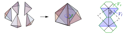
Figure 1: The deficit angle at an edge, and a cross section of the region around an edge showing the vertex and edge volumes.

On a smooth manifold $M$, the Ricci flow changes the metric $g$ according to the Ricci curvature $Rc$ at each point, with an optional second term giving a normalized Ricci flow,

$$\frac{dg}{dt}=-2Rc\,,\qquad{\text{o}r}\qquad\frac{dg}{dt}=-2Rc+\frac{2}{3}\widetilde{R}_{M}\,g\,,$$ (2.2)

where the volume can be kept constant with the use of the average scalar curvature $\widetilde{R}$ of the manifold. Both equations tend to reduce the value of the metric components associated with high positive Ricci curvature and increase those associated with high negative Ricci curvature, with the rate depending on the strength of the curvature. It was shown in [17] that the effect of the Ricci flow on the lengths of geodesic segments can be given by the integral of the Ricci curvature tangent to the segment at each point. This naturally leads to a piecewise flat approximation of the smooth Ricci flow as a set of independent equations for the fractional change in the edge-lengths,

$$\frac{1}{|\ell|}\frac{d|\ell|}{dt}=-Rc_{\ell}\,,\qquad\frac{1}{|\ell|}\frac{d|\ell|}{dt}=-Rc_{\ell}+\frac{1}{3}\widetilde{R}_{S}\,,$$ (2.3)

for a piecewise flat approximation $Rc_{\ell}$ and an average scalar curvature $\widetilde{R}_{S}$ over the piecewise flat manifold $S$. These equations will continue to give a good approximation for the smooth Ricci flow as long as the lattice gives uniformly small deficit angles.

All that remains is to give a piecewise flat approximation for the average Ricci curvature along each geodesic segment, and the average scalar curvature over the piecewise flat manifold. The first is given in terms of the sectional curvature $K_{\ell}^{\perp}$ orthogonal to the edge $\ell$, and the scalar curvature $R_{v}$ at the vertices $v_{1}$ and $v_{2}$ bounding $\ell$. These are in turn defined over volumes $V_{v}$ and $V_{\ell}$ associated with the vertex $v$ and edge $\ell$ respectively, which will be defined shortly. From [17],

$$Rc_{\ell} =\frac{1}{4}(R_{v_{1}}+R_{v_{2}})-K_{\ell}^{\perp}\,,$$ (2.4a)

$$K_{\ell}^{\perp} =\frac{1}{V_{\ell}}\left(|\ell|\,\epsilon_{\ell}+\sum_{j}\frac{1}{2}|\ell_{j}|\cos^{2}(\theta_{j})\epsilon_{j}\right),$$ (2.4b)

$$R_{v}\ =\frac{1}{V_{v}}\sum_{i}|\ell_{i}|\,\epsilon_{i}\,,\qquad\widetilde{R}_{S}=\frac{2}{V_{S}}\sum_{i}|\ell_{i}|\,\epsilon_{i}\,.$$ (2.4c)

The indices $i$, $j$ correspond to the edges intersecting the volumes $V_{v}$ and $V_{\ell}$ respectively, with $\epsilon_{i}$, $\epsilon_{j}$ representing deficit angles and $\theta_{j}$ giving the angle between $\ell_{j}$ and the edge $\ell$. The expressions for $K_{\ell}^{\perp}$ and $R_{v}$ were found by constructing volume-integrals of each curvature, with the deficit angles shown to represent local surface-integrals of the sectional curvature, and then divided by the volume to give an average. The expression for $\widetilde{R}_{S}$ can also be seen to come directly from the Regge action [15], divided by the volume $V_{S}$ of the piecewise flat manifold.

The volumes $V_{v}$ and $V_{\ell}$ are specifically chosen to ensure that the expressions above are stable to small perturbations of the volume boundaries, or of the lattice itself, and contain a large enough sampling of edges and deficit angles. As such, the vertex volumes $V_{v}$ are defined to form a dual tessellation of the piecewise flat manifold, with barycentric volumes used for the computations in this paper. The edge-volumes $V_{\ell}$ are defined as the union of the vertex volumes on either end of the edge, bounded by surfaces which are orthogonal to $\ell$ at each vertex. A cross-section of these volumes can be seen in figure 1.

Computations in [17] have successfully shown these expressions to converge to their corresponding smooth curvature values as the mesh resolution is increased, for a variety of different manifolds, and provide good approximations for reasonably sized meshes. The computations in this paper should provide even more support for the effectiveness of these piecewise flat curvature expressions. Similar expressions have also been developed for the extrinsic curvature on piecewise flat manifolds using the same approach [21], with computations also showing good approximation of, and convergence to, their corresponding smooth curvatures.

2.2   Triangulation types

For the purposes of this paper, a triangulation-type is defined as a family of simplicial graphs on a manifold, where the number of tetrahedra can be scaled in some regular way by choosing different members of the family. This scaling provides control over mesh refinements and is used to show the convergence of piecewise flat constructions to their smooth counterparts. In this section, three such triangulation types will be defined on a three-torus ($T^{3}$) topology, with a fundamental domain of size $[0,1]^{3}$ for a set of coordinates $x$, $y$, $z$. These can be directly applied to most of the manifolds, with minor adjustments required in some cases. The three different triangulation types provide a variety of edge orientations, ensuring that computation results are not based on favourable alignments alone, and provide differing levels of suitability for different dual tessellations. The building blocks for each triangulation type are defined below, and shown in figure 2.

1. The cubic block is cube-shaped and composed of six tetrahedra. There are seven edges for a given vertex, three along the $x$, $y$ and $z$ coordinates, three face-diagonals and a body-diagonal, with the tetrahedra specified so that the orientation of the face-diagonals on opposite sides agree. This is the most simple construction but it only borders on being a Delaunay triangulation for a flat metric, with the circumcenters of all six tetrahedra coinciding at the centre of the cube.

2. A skew block has the same structure as the cubic block, but with the vertices in the $x$ and $z$ directions skewed so that $v_{x}=(1,-1/3,0)$ and $v_{z}=(-1/3,-2/9,1)$. This block forms a different tiling of $T^{3}$, and gives a strongly Delaunay triangulation for a flat metric.

3. A diamond block is constructed by forming a set of four tetrahedra in a diamond shape around each coordinate edge, with the edges in the outer ring parallel with the other coordinate directions. This block contains two distinct vertices, instead of the single vertex for the other two blocks, and 14 edges, six that are parallel with the three coordinates and eight forming a set of four body-diagonal-type edges.

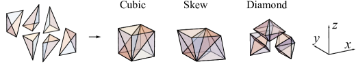
Figure 2: The three different block types, with a slight separation of the three diamond shapes forming the diamond block, and the six tetrahedra of the cubic block on the far left.

In each case, a single block can be used as a simplicial graph of $T^{3}$ by identifying faces on opposite sides. A regular grid of blocks can then be used to refine the mesh, with faces on opposite sides of the grid identified. Once the graph has been defined the vertices can be labelled, with each edge, triangle and tetrahedron then specified by the list of vertices in its closure. Since ambiguities in labelling can arise for grids that have less than three vertices in a single direction (for example all vertices in a single cubic block will have the same label), in these cases the grid is duplicated to form a slightly larger covering space before labelling, with any geometric information also duplicated but not the computations.

Unfortunately the piecewise flat Ricci flow equations are not stable when applied directly to the cubic and skew triangulation-types, but this instability can be avoided by treating the interior of each block as flat. In practice this is done be re-defining the body-diagonal edge-lengths so that the deficit angles at these edges are essentially zero. The piecewise flat Ricci flow is still performed on a simplicial triangulation, where dihedral angles and volumes can be computed in a standard way, but with the lengths of the body-diagonals adjusted for each time-step to give an essentially flat interior for each block. Using this approach, there have been no instabilities in any of the piecewise flat Ricci flow computations performed in this article. Details of the instability and proofs for the stabilizing method will be provided in a related paper.

Remark 1.

The true advantage of piecewise flat approximations is in the complete encoding of the topology in the simplicial graph. Once the boundary identifications have been made and the labels assigned, the boundaries vanish. There are no boundary conditions required for functions on piecewise flat manifolds, since the graph already has the appropriate topology. There is also no need for any coordinate systems, once geodesic lengths have been computed they just become properties of the graph. As well as avoiding coordinate singularities or translations between multiple charts, the geometry is also clear from the lengths of the edges and does not need to be separated from the characteristics of a coordinate system. This even led Tullio Regge to title his 1961 paper [15] as “General relativity without coordinates”.

3   Nil manifolds

3.1   Smooth manifold

Thurston’s geometrization conjecture states that any closed 3-manifold can be decomposed into a set of irreducible parts, each of which admits a locally homogeneous geometry. The universal covers of these geometries form a set of eight model geometries, one of which is the Nil geometry, the geometry of the continuous Heisenberg group. The Heisenberg group is a nilpotent Lie group, and can be represented by the group of $3\times 3$ matrices of the form

$$\left(\begin{array}[]{ccc}1&x&z\\ 0&1&y\\ 0&0&1\end{array}\right)$$ (3.1)

with real number entries $x$, $y$ and $z$, which can then be seen as a set of coordinates on $\mathbb{R}^{3}$.

Analytic solutions for the normalized Ricci flow of the Nil geometry were first given by Isenberg and Jackson [18], with the quasi-convergence of the non-normalized Ricci flow later studied by Knopf and McLeod [19]. These approaches make use of work by Milnor [22] and by Ryan and Shepley [23], where an orthogonal frame of 1-forms $\{\theta^{a}\}$ can be found in which the metric is diagonal

$$g=A(\theta^{1})^{2}+B(\theta^{2})^{2}+C(\theta^{3})^{2},$$ (3.2)

and the structure constants $C^{a}_{bd}$ (such that $d\theta^{a}=C^{a}_{bd}\theta^{b}\wedge\theta^{d}$) are all zero except for $C^{1}_{23}=-C^{1}_{32}=\lambda$, for some constant $\lambda$. The Ricci curvature is also diagonal in this frame, which reduces both the normalized and non-normalized Ricci flows to a set of ordinary differential equations for the metric components $A$, $B$ and $C$, with the frame and structure constants invariant to the flows. The constant $\lambda$ can be seen as a scaling factor on the $z$ coordinate in the matrix representation of the Heisenberg group (3.1),

$$\left(\begin{array}[]{ccc}1&x&z/\lambda\\ 0&1&y\\ 0&0&1\end{array}\right).$$ (3.3)

In [18] this constant is taken as the volume element ($\lambda=\sqrt{ABC}$), coming from a weighted Levi-Civita antisymmetric tensor in equation (4), which is invariant under the volume-preserving normalized Ricci flow. Solutions for $A$, $B$ and $C$ are then given in equations (29). A value of $-2$ is used for $\lambda$ in [19], with solutions for the non-normalized Ricci flow given in equations (15). The latter solutions can also be found in the Ricci flow textbooks [24, 25], in equations (1.8) and (4.62) respectively.

It can easily be shown that the scalar curvature $R=-\frac{\lambda^{2}A}{2BC}$, with solutions for the metric functions under the normalized Ricci flow then given by the equations:

$$A=A_{0}\left(1-\frac{16}{3}R_{0}t\right)^{-1/2},\quad B=B_{0}\left(1-\frac{16}{3}R_{0}t\right)^{1/4},\quad C=C_{0}\left(1-\frac{16}{3}R_{0}t\right)^{1/4},$$ (3.4)

and under the non-normalized Ricci flow by:

$$A=A_{0}(1-6R_{0}t)^{-1/3},\quad B=B_{0}(1-6R_{0}t)^{1/3},\quad C=C_{0}(1-6R_{0}t)^{1/3},$$ (3.5)

for initial values $A_{0}$, $B_{0}$ and $C_{0}$, and the initial scalar curvature $R_{0}=-\frac{\lambda^{2}A_{0}}{2B_{0}C_{0}}$. The normalized Ricci flow solutions agree with those of [18] for $\lambda=\sqrt{ABC}$, and the non-normalized solutions agree with [19] for $\lambda=-2$.

For computational purposes, the initial metric (3.2) is chosen so that $A_{0}=B_{0}=C_{0}=1$. In the coordinates given by the matrix representation of the Heisenberg group in equation (3.3), the metric takes the form

$$ds^{2}=dx^{2}+dy^{2}+(dz+\lambda\,x\,dy)^{2}.$$ (3.6)

The orthogonal frame is obtained from these coordinates by the identification $\{\theta^{1},\theta^{2},\theta^{3}\}=\{dz,dy+\lambda\,x\,dz,dx\}$. In order to obtain a compact computational domain, the continuous Heisenberg group can be quotiented by the finite Heisenberg group, with integer entries in the upper-right triangle. This gives a fundamental domain with the $x$ and $y$ coordinates having a range of $[0,1]$ and the $z$ coordinate a range of $[0,\lambda]$. The $yz$ planes have a two-torus topology, while the identification of the $yz$ faces at $x=0$ and $x=1$ requires a sort of twist, as shown in figure 3.

3.2   Triangulating manifold

For a single cubic block triangulation, the decomposition into six tetrahedra is done in a slightly different way to section 2.2, see figure 3, so that the face-diagonals match the face relations for the fundamental domain. The geometry is isometric in the $yz$-planes, with a standard two-torus topology, so triangulations only require a single block in the $y$ and $z$ directions. Although the Nil geometry is completely homogeneous, the metric representation in (3.6) depends on the $x$-coordinate, so increased resolutions are given by joining copies of the standard cubic block along the $x$-direction, with the complete collection of blocks still spanning $[0,1]$. This has the effect of sub-dividing the twist into multiple parts, and reduces the size of the deficit angles. Vertices, edges and triangles on opposite faces are then identified, paying attention to the $yz$-face relations. Adapting the skew and diamond triangulation types to the Nil face relations is not so straight forward, so only the cubic triangulation type will be used here. However, since the $y$-edges are not orthogonal to the $z$-edges beyond $x=0$, each block in the grid can be considered as a slightly different triangulation type.

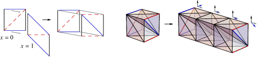
Figure 3: Relations between the $yz$-faces at $x=0$ and $x=1$ for $\lambda=1$, and single and three-block triangulations with these face relations. The orthogonal frames for $\{\theta^{i}\}$ are also indicated for different values of $x$ along the three-block triangulation.

In order to compare with the analytic results of Isenberg & Jackson [18] and Knopf & McLeod [19], the normalized Ricci flow is computed for triangulations with $\lambda=1$ and the non-normalized Ricci flow for triangulations with $\lambda=-2$. Grids of one, two and three blocks are then used for both situations. For the $\lambda=1$ case, these triangulations have a range of $[0,1]$, $[0,1/2]$ and $[0,1/3]$ respectively in the $y$ and $z$ directions, in order to keep the tetrahedra close to regular. The original domain can then be recovered with four and nine copies for the two and three block triangulations. For the $\lambda=-2$ case, the twist is in the opposite direction, so the triangulations are a reflection in the $xy$-plane of those shown in figure 3. A range of $[0,1/2]$ is used in the $x$-direction here, to keep from stretching the cubes too much, with the $y$ and $z$ directions given ranges of $[0,1/2]$, $[0,1/4]$ and $[0,1/6]$ for the three different grid sizes. Again, the original domain can be recovered with grids of copies with dimensions $2\times 2\times 4$, $2\times 4\times 8$ and $2\times 6\times 12$ in the $x$, $y$ and $z$ directions.

3.3   Results of evolutions

Evolutions of the normalized and non-normalized piecewise flat Ricci flow (2.3) are computed using the Euler method, with 120 steps of size 0.005 for each triangulation. Since Nil manifolds are homogeneous, the values of the metric functions can be given by the square of the geodesic lengths for a unit coordinate length in the $x$ and $z$ directions for $C$ and $A$ respectively, and in the $y$-direction at $x=0$ for $B$. The resulting values are graphed in figure 4 as piecewise linear curves, along with the analytic solutions from equations (3.4) and (3.5). The piecewise flat curves can be seen to give good approximations for the analytic solutions, even for the single block triangulations with only six tetrahedra, and there is a clear convergence to the analytic solutions as the number of blocks is increased.

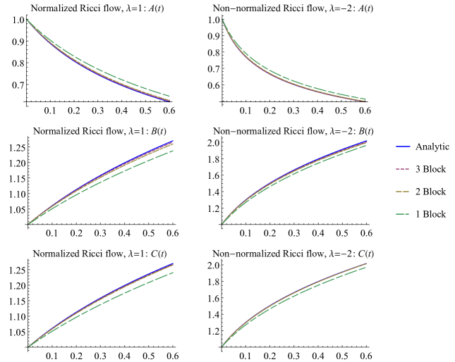
Figure 4: Graphs of the metric functions in time for both the normalized and non-normalized Ricci flows, all showing convergence to the analytic solutions as the resolution is increased.

The piecewise flat values for $A$, $B$ and $C$ have also been fitted to a general function matching the form of the analytic equations (3.4) and (3.5),

$$f(t)=(1+a\,t)^{b}.$$ (3.7)

The resulting best-fit parameters for $a$ and $b$ are shown in table 1, for each of the functions and both evolutions, with $R$-squared values of greater than $0.999999$ in all cases. These again show a clear convergence to the analytic solutions from [18] and [19], as the resolution is increased, with very close approximations for the three-block triangulations in particular.

	A		B		C
Normalized	a	b	a	b	a	b
1-Block	$2.037$	$-0.547$	$2.057$	$0.265$	$2.029$	$0.270$
2-Block	$2.460$	$-0.515$	$2.578$	$0.247$	$2.449$	$0.260$
3-Block	$2.585$	$-0.506$	$2.674$	$0.246$	$2.596$	$0.252$
Analytic	$2.667$	$-0.5$	$2.667$	$0.25$	$2.667$	$0.25$
Non-norm.	a	b	a	b	a	b
1-Block	$9.50$	$-0.352$	$9.88$	$0.348$	$9.68$	$0.354$
2-Block	$11.43$	$-0.338$	$11.67$	$0.332$	$11.48$	$0.339$
3-Block	$11.94$	$-0.335$	$12.14$	$0.329$	$11.92$	$0.334$
Analytic	$12$	$-0.333$	$12$	$0.333$	$12$	$0.333$

Table 1: The best fit parameters for expressions of the form (3.7), showing a clear convergence to the analytic solutions, with $R$-squared values greater than $0.999999$ in all cases.

4   Gowdy manifold

4.1   Smooth manifold

The Gowdy manifolds are a family of 3-geometries that can be foliated into isometric 2-surfaces and are periodic in the direction orthogonal to these surfaces. These manifolds first appeared as the spatial part of a cosmological space-time model introduced by Robert Gowdy [26], with dynamics capable of containing gravitational waves. They were then used by Carfora, Isenberg and Jackson [20] to show that the Ricci flow can be convergent for manifolds with non-positive-definite curvature. With coordinates $x$ and $y$ spanning the isometric 2-surfaces, and $\theta$ orthogonal to them, the metric can be written in the general form

$$ds^{2}=e^{f+W}dx^{2}+e^{f-W}dy^{2}+e^{2a}d\theta^{2}\,,$$ (4.1)

with a constant function $f$, and functions $W$ and $a$ depending on the value of $\theta$. The non-normalized Ricci flow of this metric can be represented by a coupled set of partial differential equations (PDEs) for these functions:

$$\partial_{t}f=0,\quad\partial_{t}a=\frac{1}{2}e^{-2a}\left(\partial_{\theta}W\right)^{2},\quad\partial_{t}W=e^{-2a}\left(\partial_{\theta}^{2}W-\partial_{\theta}a\cdot\partial_{\theta}W\right).$$ (4.2)

These equations were easily solved numerically for initial-time functions

$$f_{0}=0,\qquad a_{0}=0,\qquad W_{0}=0.1\sin\theta,$$ (4.3)

requiring nothing more than the built-in PDE solver in Mathematica. The normalized Ricci flow equations are not so straight forward to solve, particularly in ensuring that $f$ is constant for each value of $t$. As a result, only the non-normalized Ricci flow is investigated here, though the volume is also close to being invariant for the non-normalized flow. It should be noted that there is no extra difficulty in computing the piecewise flat normalized Ricci flow.

4.2   Triangulating manifold

The Gowdy manifold is the simply connected covering space of a compact $T^{3}$ manifold with fundamental domain $[0,s_{x}]\times[0,s_{y}]\times[0,2\pi]$, for any values $s_{x}$ and $s_{y}$. This can be used as a compact domain for the piecewise flat computations. Since the manifold is isometric in each $xy$-plane, triangulations only require a single block in the $x$ and $y$ directions. Different resolutions for cubic and skew triangulation types are provided by grids of $6$, $12$ and $24$ blocks in the $\theta$ direction, with $3$, $6$ and $12$ diamond blocks having the same number of vertices and edges. To keep the tetrahedra close to regular, both $s_{x}$ and $s_{y}$ are chosen to be $2$, $1$, $1\over 2$ and $1\over 4$ for the $3$, $6$, $12$ and $24$ block grids respectively, with $4$, $16$ and $64$ copies of the latter three grids giving the same domain for all triangulations. The piecewise flat curvatures for the cubic and skew triangulations have already been shown in [17] for the initial manifold.

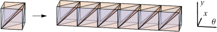
Figure 5: A grid of six cubic blocks along the $\theta$-direction for the lowest resolution triangulation, with the vertices, edges and triangles on opposite sides identified to give a $T^{3}$ topology.

4.3   Results of evolutions

The piecewise flat Ricci flow (2.3) was applied to each of the triangulations, using the Euler method with $35$ time-steps of size $0.02$. Piecewise-linear graphs for the flow of the piecewise flat scalar curvature at $\theta=\pi/3$ are shown on the left-hand side of figure 6, together with the scalar curvature from the numerical PDE solution. The right-hand side of the figure shows the Ricci curvatures along the $y$-direction at $\theta=\pi/3$. The $\theta$ value of $\pi/3$ was chosen since the initial curvatures are all non-zero here, and there is a vertex at this value of $\theta$ for all of the triangulations. The $y$-edge was selected for the Ricci curvature as this is the only edge that is part of all three triangulation types. The graphs show convergence to the PDE solutions for both curvatures and all three triangulation types as the resolution is increased. For each resolution, the curves are also almost exactly the same across all three triangulation types, aside from the scalar curvature for the diamond type triangulations.

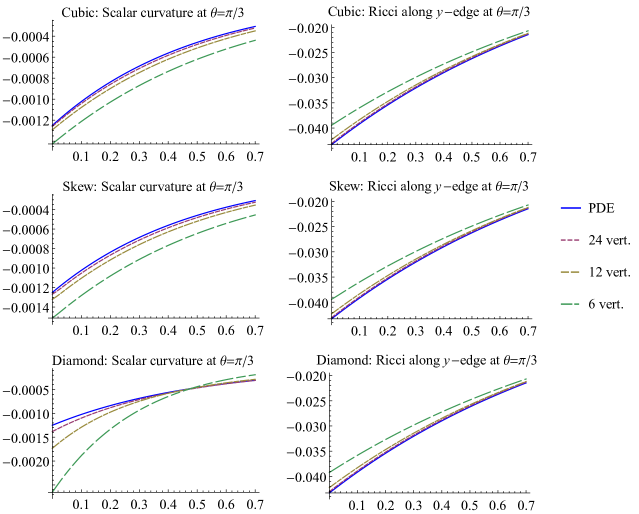
Figure 6: Piecewise-linear graphs of the curvature values in time, showing a clear convergence of the piecewise flat to the PDE solution as the resolution is increased.

Since it was shown that the curvature decays exponentially to zero by Carfora et al. [20], exponential functions were fitted to the time evolution of the scalar and Ricci curvatures graphed in figure 6, with the decay rates for the best-fit functions shown in table 2. Each column can be seen to converge to the PDE value, with good approximations for even the lowest resolutions, and very similar values for each resolution across all three triangulation types, particularly for the Ricci curvature. The $R$-squared values of the fitted functions are greater than $0.99999$ for all but the scalar curvatures of the diamond triangulations, which are no lower than $0.9997$. The larger errors and lower $R$-squared values may be due to the overlapping of edges along the $\theta$-direction for the diamond blocks, giving a larger $\theta$-interval for the averaging of the scalar curvature and requiring more blocks to resolve it better.

	Cubic		Skew		Diamond
	$R$	$Rc$	$R$	$Rc$	$R$	$Rc$
6-vertices	$1.673$	$0.921$	$1.714$	$0.921$	$3.57$	$0.915$
12-vertices	$1.856$	$0.988$	$1.880$	$0.989$	$2.67$	$0.986$
24-vertices	$1.941$	$1.006$	$1.950$	$1.006$	$2.156$	$1.005$
PDE solution	$2.003$	$1.003$	$2.003$	$1.003$	$2.003$	$1.003$

Table 2: Decay rates for the best-fit exponential functions of the scalar curvature and the Ricci curvature along the $y$-direction, both at $\theta=\pi/3$. The $R$-squared values are at least $0.99999$ for all but the diamond scalar curvatures, and each column shows a convergence to the corresponding PDE value as the resolution is increased.

Visual representations of the Ricci curvature as a function of $\theta$ are shown in figure 7 for times $t=0$ and $t=0.7$, with different edges used for each triangulation type. The $\theta$-coordinate was selected for the cubic triangulations, since $Rc(\hat{\theta},\hat{\theta})\equiv-R$, corresponding with the scalar curvature in figure 6 and table 2 above. The $y$-edge was chosen for the diamond triangulation type, corresponding to the Ricci curvature in figure 6 and table 2, and the body-diagonal for the skew triangulations. All six graphs show good approximations for all resolutions, and a convergence to the PDE curves as the resolutions are increased. The shape of the first two sets of graphs remain mostly unchanged, with the scale decreasing by about a quarter and a half respectively, agreeing with the decay rates in table 2. Despite the lengths of the body-diagonals being re-defined to give zero deficit angles, required for the stability of the flow as mentioned at the end of section 2.2, the piecewise flat curves are no further from the PDE curve than for the other edges. This reinforces the robustness of the curvature constructions in (2.4). These curves also show the piecewise flat Ricci flow producing more than just a scale change, with the change in shape between the two times resulting from a change in the orientation of the edges, which is perfectly matched by the piecewise flat curvatures.

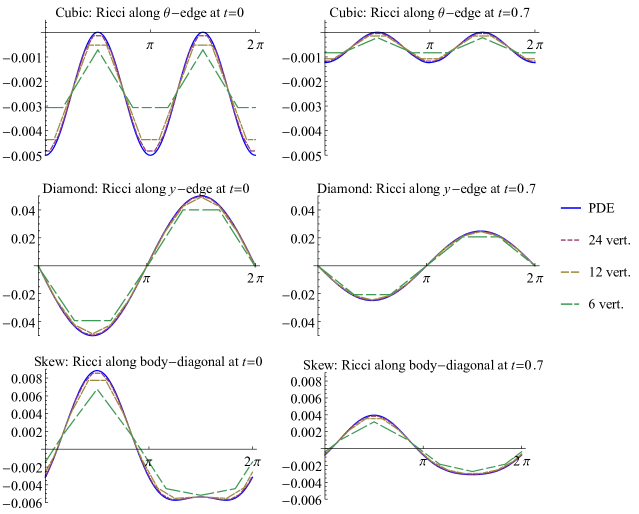
Figure 7: Graphs of the Ricci curvature as a function of $\theta$, for $t=0$ and $t=0.7$, showing convergence to the PDE solutions as the resolution is increased in all cases.

To show that the edges graphed in figure 7 are not special cases, the errors for the Ricci curvatures were computed at all edges for both $t=0$ and $t=0.7$, with respect to the corresponding PDE solution values. There is evidence that the errors scale with the overall curvature of the manifold, so the mean absolute values of the errors are given as percentages of an average of the Ricci curvature for the corresponding value of $t$. This average is found by first taking the square-root of the tensor square of the Ricci curvature and then averaging over $\theta$,

$$Rc_{\textrm{a}ve}:=\frac{1}{2\pi}\int_{0}^{2\pi}\sqrt{Rc^{2}}\,d\theta\,.$$ (4.4)

In table 3, these percentage errors can be seen to decrease in all cases as the resolution is increased. The errors also have similar values across all triangulation types, showing a certain level of independence to this choice for both the curvature values and the Ricci flow.

	Cubic		Skew		Diamond
	$t=0$	$t=0.7$	$t=0$	$t=0.7$	$t=0$	$t=0.7$
6-Vertices	$12.4\%$	$7.4\%$	$9.0\%$	$5.4\%$	$9.0\%$	$3.5\%$
12-Vertices	$3.3\%$	$2.4\%$	$2.5\%$	$2.1\%$	$2.7\%$	$1.2\%$
24-Vertices	$0.8\%$	$1.2\%$	$1.1\%$	$1.4\%$	$0.8\%$	$0.7\%$

Table 3: The mean absolute error of the Ricci curvature over all edges in each triangulation, as a percentage of the mean absolute value of the curvature at each time (4.4), showing a decrease everywhere as the resolution is increased.

There is a notable reduction in the errors from $t=0$ to $t=0.7$ for the lower resolution triangulations, the top row of table 3. This is likely due to the under-approximation of the initial curvature magnitudes, as seen in figure 7, giving a slower decay rate and reducing these errors in time. The effect indicates a general stabilizing behaviour in the piecewise flat Ricci flow, with errors reducing over time, at least for manifolds where the curvature magnitude is decreasing everywhere.

5   Three-torus initially embedded in $\mathbb{E}^{4}$

5.1   Smooth manifold

A regular three-torus can be embedded in Euclidean four-space $\mathbb{E}^{4}$ by beginning with a circle of radius $r_{\theta}$ and rotating it around another circle of radius $r_{\phi}>r_{\theta}$ in a plane orthogonal to it. The resulting two-torus can then be rotated around a third circle with radius $r_{\psi}>r_{\phi}$, in a plane orthogonal to both of the previous circles. For a poloidal-type coordinate system, with angular coordinates $\theta$, $\phi$ and $\psi$ for each circle, the metric induced by the embedding is

$$ds^{2}=r_{\theta}^{2}\ d\theta^{2}+(r_{\phi}+\cos\theta)^{2}\ d\phi^{2}+(r_{\psi}+(r_{\phi}+\cos\theta)\cos\phi)^{2}\ d\psi^{2}\ .$$ (5.1)

This manifold is isometric along the $\psi$-coordinate, and the integral curves of the $\theta$-coordinate vector fields are the same everywhere, with values of $2\pi r_{\theta}$. The minimum and maximum $\phi$ integral curves have lengths $2\pi(r_{\phi}-r_{\theta})$ and $2\pi(r_{\phi}+r_{\theta})$ with minimum and maximum lengths of $2\pi(r_{\psi}-r_{\phi})$ and $2\pi(r_{\psi}+r_{\phi})$ for the $\psi$ integral curves. These can be seen as generalizations of the inner and outer perimeters of a two-torus in $\mathbb{E}^{3}$, as shown in figure 8. The smooth Ricci flow of the metric above is expected to tend asymptotically to a flat three-torus, with the minimum and maximum orbits both approaching the same value asymptotically, for each coordinate.

5.2   Triangulating manifold

For the piecewise flat computations, the radii were chosen to have the values

$$r_{\theta}=1\,,\qquad r_{\phi}=2\,,\qquad r_{\psi}=4\,.$$ (5.2)

Since the manifold is isometric in the $\psi$-direction, only a single layer of blocks in a $\theta\phi$-plane is required. For the cubic block, grids of size $4\times 6$, $6\times 6$ and $6\times 8$ are used, with grids of size $3\times 4$, $4\times 4$ and $4\times 5$ for the diamond block. These give the same number of vertices and edges for the smallest and largest grids for both triangulation types. The entire range of the $\theta$ and $\phi$ coordinates is covered by all triangulations, but to keep the blocks regular in shape only $1/(2n_{x})$ of the $\psi$-coordinate, where $n_{x}$ is the number of blocks along the $\theta$-direction. This means that $8$, $12$ and $12$ copies of the cubic triangulations will be needed to cover the entire manifold, and $6$, $8$ and $8$ copies of the diamond triangulations. Unfortunately, the skew triangulation would require at least three layers of blocks in the $\psi$-direction in order to have vertices and edges on opposite sides match, so only the cubic and diamond triangulation types are used for this manifold.

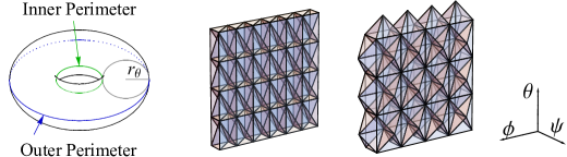
Figure 8: A two-torus embedded in $\mathbb{E}^{3}$, showing the inner and outer perimeters tangent to the $\phi$-coordinate vector fields, and the lowest resolution grids for both the cubic and diamond triangulation types, with opposite sides identified to form a $T^{3}$ topology.

5.3   Results of evolution

The triangulations are evolved according to the non-normalized piecewise flat Ricci flow equations (2.3), using the Euler method with $80$ steps of size $0.05$. In order to help visualize the flow, the lengths of the edges along both the minimum and maximum $\phi$ and $\psi$ integral curves are summed for each time step. Although the $\theta$ integral curves all have equivalent lengths to begin with, the Ricci curvatures are not invariant along the $\phi$-coordinate, so different length curves emerge with the flow. The total lengths of the minimum and maximum integral curves in time, for all three resolutions, are graphed together in figure 9 for each coordinate and each triangulation type.

The graphs show the integral curve lengths converging asymptotically toward the same value for each coordinate, indicating that the manifold is flowing toward a three-torus with consistent dimensions. The values at $t=4$ are also given in table 4, providing bounds for the final three-torus dimensions for each triangulation. Both the curves and table values can also be seen to converge to the same shape and values for both triangulation types as the resolution is increased, sometimes from different directions. This suggests that the higher resolution values are closer to the smooth values, with both triangulation types agreeing to certain levels of precision.

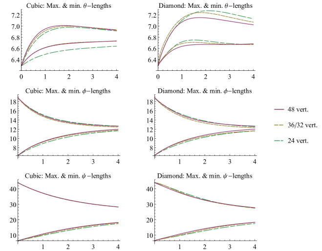
Figure 9: The flow of the maximum and minimum integral curve lengths for each coordinate, tending asymptotically toward the same value in all cases. The curves for both triangulation types also tend to converge to the same shape and values as the resolutions are increased.

	$\theta$		$\phi$		$\psi$
Cubic	Min	Max	Min	Max	Min	Max
24-Block	$6.639$	$6.912$	$11.67$	$12.70$	$17.36$	$28.16$
36-Block	$6.729$	$6.934$	$11.81$	$12.48$	$17.89$	$28.26$
48-Block	$6.734$	$6.925$	$12.00$	$12.66$	$18.14$	$28.23$
Diamond	Min	Max	Min	Max	Min	Max
12-Block	$6.668$	$7.132$	$11.65$	$12.55$	$17.51$	$27.44$
16-Block	$6.672$	$7.072$	$11.68$	$12.34$	$18.22$	$27.58$
24-Block	$6.682$	$7.024$	$12.02$	$12.69$	$18.28$	$27.77$

Table 4: The minimum and maximum perimeter lengths at $t=4$, bounding the dimensions of the limiting flat three-torus, with both triangulation types tending towards the same values.

To show that the manifold is actually flowing to a flat three-torus, the average of the absolute values of both the Ricci curvature and deficit angles, weighted by the edge-lengths, are also computed for each time step. The equations for these averages are

$$\widetilde{Rc_{\ell}}:=\frac{\sum_{\ell}|\ell||Rc_{\ell}|}{\sum_{\ell}|\ell|}\ ,\qquad\widetilde{\epsilon_{\ell}}:=\frac{\sum_{\ell}|\ell||\epsilon_{\ell}|}{\sum_{\ell}|\ell|}\ .$$ (5.3)

The results are graphed in figure 10, showing that both flow asymptotically to zero. The deficit angles can also be seen to reduce as the resolution is increased, for both triangulation types and at all times.

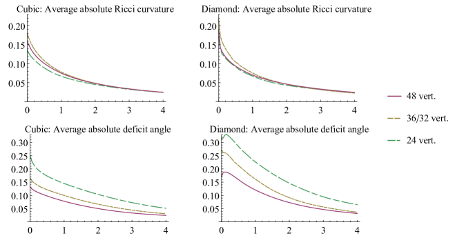
Figure 10: The average magnitudes of both the Ricci curvature and deficit angles, all tending asymptotically to zero. The Ricci curvature also tends toward the same curve for both triangulation types, and the deficit angles are smaller for increased resolutions at all times.

6   Perturbation of a flat three-torus

6.1   Smooth manifold

A simple perturbation of a flat three-torus has been used to give a manifold without any continuous isometries. For a three-torus topology, with coordinates $x$, $y$ and $z$ ranging from $0$ to $1$, the metric was chosen to be

$$ds^{2}=(1+0.2\sin(\pi x)\sin(\pi y)\sin(\pi z))\left(dx^{2}+dy^{2}+dz^{2}\right)\ .$$ (6.1)

As with both the Gowdy manifold and the three-torus, this manifold is expected to Ricci flow asymptotically back to a flat three-torus.

6.2   Triangulating manifold

Without any continuous isometries, there are no reductions that can be made for the triangulation grids. The cubic blocks are arranged in grids of size $2^{3}$, $3^{3}$ and $4^{3}$, with the diamond type triangulations starting at a single block with grids of size $2^{3}$ and $3^{3}$ as well. The vertices and edges of the skew blocks must align with other vertices and edges when opposite faces are identified. To make this easier for smaller grid sizes the skew block is adapted a little with the vertices in the $x$ and $z$ directions skewed so that $v_{x}=(1,-1/2,0)$ and $v_{z}=(-1/2,-1/4,1)$. This still requires even numbers of blocks in each direction, so only two grids of size $2\times 2\times 2$ and $4\times 4\times 4$ are used.

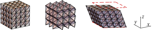
Figure 11: The highest resolution grids for the cubic, diamond and skew triangulation types, with the identification between the two $xy$-faces indicated for the skew triangulation.

6.3   Results of evolution

The triangulations are evolved using the Euler method, with $50$ steps of size $0.002$, for the non-normalized piecewise flat Ricci flow. The smooth manifold is expected to flow asymptotically to a flat three-torus, so the lengths of the integral curves for each coordinate should all converge to the same value. Though the manifold does not have any continuous isometries, it is discretely symmetric for any permutation of the coordinates, so the three sets of coordinate integral curves should be equivalent. Since all three triangulation types have edges aligned with the $y$-coordinate, the minimum and maximum lengths of the $y$ integral curves have been computed for each time step, and are graphed on the left-hand side of figure 12.

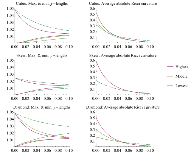
Figure 12: On the left, the minimum and maximum integral curve lengths along the $y$-coordinate show convergence to the same value for each triangulation type. The graphs on the right show the curvature flowing asymptotically to zero, and tending to the same shape for all three triangulation types as the resolution is increased.

For the initial smooth manifold, the minimum integral curve lengths occur at $(x,z)=(0,0)$ and the maximum lengths at $(x,z)=(0.5,0.5)$. All of the triangulations have edges along the minimum-length integral curves, and the graphs show convergence to the same time-curve as the resolutions are increased. The middle resolution cubic triangulation time-curve has been omitted from the graph, since there are no $y$-edges at $(x,z)=(0.5,0.5)$, and the skew triangulations use a set of edges that are slightly offset, giving shallower curves for the middle graph on the left-hand side of figure 12. The curves for the maximum and minimum lengths tend asymptotically to the same value for all of the triangulations, indicating that the manifold tends to a three-torus with consistent dimensions. The values of these lengths at $t=0.1$ are also given in table 5, giving bounds for the dimensions of the limiting manifold, with both the minimum and maximum values converging towards similar values for all three triangulation types as the resolution is increased.

	Cubic		Skew		Diamond
Resolutions	Min	Max	Min	Max	Min	Max
Lowest	$1.0074$	$1.0177$	$1.0096$	$1.0148$	$1.0190$	$1.0290$
Middle	$1.0106$	$-$	$-$	$-$	$1.0117$	$1.0139$
Highest	$1.0114$	$1.0133$	$1.0115$	$1.0129$	$1.0118$	$1.0131$

Table 5: Values for both the minimum and maximum lengths in the $y$-direction at $t=0.1$, giving bounds on the dimensions of the limiting flat three-torus for each approximation.

The right-hand side of figure 12 shows the average magnitude of the Ricci curvature over all the edges of each triangulation, according to equation (5.3). These also show the Ricci flow is tending towards a flat manifold, with all three triangulation types tending towards the same time-curves as the resolution is increased.

7   Conclusion

The computations in sections 3 to 6 have successfully demonstrated the effectiveness of the piecewise flat Ricci flow introduced in [17] for a variety of manifolds, ranging from completely homogeneous to no continuous symmetries. These computations have shown:

• a clear convergence to the smooth Ricci flow as the mesh resolution is increased,

• good approximations for the smooth flow for reasonable resolutions,

• equivalent results for different types of mesh, to appropriate levels of precision, and

• no dependence on any symmetry properties of the manifolds.

Specifically, the piecewise flat Ricci flow of the Nil manifolds converge to the analytic solutions first appearing in [18] and [19], for the normalized and non-normalized Ricci flow respectively, with errors on the order of $1\%$ for the fitted parameters in table 1 using only 18 tetrahedra. The approximations for the Gowdy manifold show convergence to a set of PDE solutions, with Ricci curvature errors of about $1\%$ at $t=0.7$ for 144 tetrahedra. For the three-torus initially embedded in $\mathbb{E}^{4}$ the average magnitude of the Ricci curvature goes to zero and the minimum and maximum lengths along each coordinate asymptotically approach each other. Finally, the perturbed flat three-torus asymptotically flows back to a flat three-torus, with all three triangulation types approaching the same bounding values for the dimensions of the limiting three-torus as the resolution is increased.

Other properties have also become apparent from some of the individual computations. Even very low resolution triangulations still give appropriate behaviour for the flow, as can be seen from the single cubic block triangulations of the Nil manifolds, and the single diamond block in figure 12, which is likely due to the topology being fixed by the piecewise flat graphs. In some cases, different triangulations can be used to give upper and lower bounds on the smooth solution, with the top two graphs in figure 9 showing time-curves for two different triangulation types approaching the same curve but from different directions. The robustness of the piecewise flat curvature constructions is particularly evident from the lower two graphs in figure 7, especially since the deficit angles are zero at these edges due to adaptations to the triangulations for stability purposes. The lower resolution triangulations in table 3 also show a robustness for the piecewise flat Ricci flow of the Gowdy model, with over-approximations of the curvature decreasing quicker and under-approximations slower, also seen in figure 7.

References

- [1] R Hamilton. Three-manifolds with positive ricci curvature. J. Differential Geom., 17 255-306, 1982.
- [2] G. Pereleman. The entropy formula for the Ricci flow and its geometric applications. arXiv:0211159.
- [3] G. Pereleman. Ricci flow with surgery on three-manifolds. arXiv:0303109.
- [4] W Zeng, X Yin, Y Zeng, Y Lai, X Gu, and D Samaras. 3D face matching and registration based on hyperbolic Ricci flow. Proc. IEEE Conf. Computer Vision on Pattern Recognition Workshop 3D Face Processing, 1-8, 2008.
- [5] W Zeng, J Marino, K Gurijala, X Gu, and A Kaufman. Supine and prone colon registration using quasi-conformal mapping. IEEE Trans. Visual. Comput. Graph., 16 1348-1357, 2010.
- [6] E Woolgar. Some applications of Ricci flow in physics. Canadian Journal of Physics, 86 4, 645-651, 2008.
- [7] M Headrick and T Wiseman. Ricci flow and black holes. Class. Quantum Grav., 23 6683-6707, 2006.
- [8] P Figueras, J Lucietti, and T Wiseman. Ricci solitons, Ricci flow and strongly coupled CFT in Schwarzschild Unruh or Boulware vacua. Class. Quantum Grav., 28 215018, 2011.
- [9] D Garfinkle and J Isenberg. Numerical studies of the behaviour of Ricci flow. In S-C Chang, B Chow, S-C Chu, and C-S Lin, editors, Geometric Evolution Equations, Contemp. Math. 367, pages 103–114. American Mathematical Society, 2005.
- [10] B Chow and F Luo. Combinatorial Ricci flows on surfaces. J. Differential Geom., 63 97-129, 2003.
- [11] J Kim, F Luo, and X Gu. Discrete surface Ricci flow. IEEE Trans. Visual. Comput. Graph., 14 1030-1043, 2008.
- [12] M Zhang, W Zeng, R Guo, F Luo, and X Gu. Survey on discrete surface Ricci flow. Journal of Computer Science and Technology, 30 3, 598-613, 2015.
- [13] D Garfinkle and J Isenberg. The modeling of degenerate neck pinch singularities in Ricci flow by Bryant solitons. Jounral of Mathematical Physics, 49 073505, 2008.
- [14] W A Miller, J R McDonald, P M Alsing, D X Gu, and S-T Yau. Simplicial Ricci flow. Commun. Math. Phys., 329, 579-608, 2014.
- [15] T Regge. General relativity without coordinates. Nuovo Cimento, 19, 558, 1961.
- [16] P M Alsing, W A Miller, M Corne, X D Gu, S Lloyd, S Ray, and S-T Yau. Simplicial Ricci flow: an example of a neck pinch singularity in 3d. Geom., Imaging Comp., 1, no. 3, 303-331, 2014.
- [17] R Conboye and W A Miller. Piecewise flat curvature and Ricci flow in three dimensions. Asian J. Math., 21 6, 1063-1098, 2017.
- [18] J Isenberg and M Jackson. Ricci flow of locally homogeneous geometries on closed manifolds. J. Differential Geom., 32 723-741, 1992.
- [19] D Knopf and K McLeod. Quasi-convergence of model geometries under the Ricci flow. Comm. Anal. Geom., 9, no. 4, 879-919, 1999.
- [20] M Carfora, J Isenberg, and M Jackson. Convergence of the Ricci flow for metrics with indefinite Ricci curvature. J. Differential Geom., 31 249-263, 1990.
- [21] R Conboye. Piecewise flat extrinsic curvature. arXiv:1612.07753, 2016.
- [22] J Milnor. Curvatures of left invariant metrics on Lie groups. Adv. Math., 21 293-329, 1976.
- [23] Michal P Jr. Ryan and Lawrence C Shepley. Homogeneous Relativistic Cosmologies. Princeton University Press, 1975.
- [24] Bennet Chow and Dan Knopf. The Ricci Flow: An Introduction. American Mathematical Society, 2004.
- [25] Bennet Chow, Peng Lu, and Lei Ni. Hamilton’s Ricci Flow. American Mathematical Society, 2006.
- [26] R Gowdy. Vacuum spacetimes with two-parameter spacelike isometry groups and compact invariant hypersurfaces. Ann. Phys., 83 203-241, 1974.