Performance of the Constrained Minimization of the Total Energy in Density Functional Approximations: the Electron Repulsion Density and Potential

Abstract

In the constrained minimization method of Gidopoulos and Lathiotakis (J. Chem. Phys. 136, 224109), the Hartree exchange and correlation Kohn-Sham potential of a finite $N$-electron system is replaced by the electrostatic potential of an effective charge density that is everywhere positive and integrates to a charge of $N-1$ electrons. The optimal effective charge density (electron repulsion density, $\rho_{\rm rep}$) and the corresponding optimal effective potential (electron repulsion potential $v_{\rm rep}$) are obtained by minimizing the electronic total energy in any density functional approximation. The two constraints are sufficient to remove the self-interaction errors from $v_{\rm rep}$, correcting its asymptotic behavior at large distances from the system. In the present work, we describe, in complete detail, the constrained minimization method, including recent refinements. We also assess its performance in removing the self-interaction errors for three popular density functional approximations, namely LDA, PBE and B3LYP, by comparing the obtained ionization energies to their experimental values for an extended set of molecules. We show that the results of the constrained minimizations are almost independent of the specific approximation with average percentage errors 15%, 14%, 13% for the above DFAs respectively. These errors are substantially smaller than the corresponding errors of the plain (unconstrained) Kohn-Sham calculations at 38%, 39% and 27% respectively. Finally, we showed that this method correctly predicts negative values for the HOMO energies of several anions.

I Introduction

It is well known that approximations in density functional theory (DFT) suffer from self-interaction (SI) errors Perdew and Zunger (1981). In the total energy, SIs arise in the Hartree (or Coulomb) term that represents the electrostatic Coulomb repulsion energy of the electronic charge density $\rho$ with itself. In theories that employ a non-interacting $N$-particle (Slater determinant) state to represent the interacting system, (like Hartree-Fock, Kohn-Sham-DFT), the charge density $\rho$ is the sum of the single-particle densities of the orbitals that form the Slater determinant.

In Hartree-Fock theory, this self repulsion is cancelled exactly for the occupied orbitals Blair et al. (2015), by the Fock exchange term. In KS DFT, the same happens with the exact exchange energy functional, $E_{x}[\rho]$, which is also based on the Fock exchange energy expression in terms of the KS orbitals. However, for approximate exchange energy functionals the cancellation of the SIs is not complete.

Self interactions have a large impact on the accuracy of many properties predicted by density functional approximations. These errors include: artificial stabilization of delocalized states Lundberg and Siegbahn (2005), underestimating electron affinities Rösch and Trickey (1997) and the underestimation of ionization energies and band gapsToher et al. (2005); Goedecker and Umrigar (1997); Perdew and Levy (1983).

The SI error is readily observed in the asymptotic behavior of the Kohn Sham (KS) potential Almbladh and von Barth (1985). For an $N$-electron system, in a theory without SIs, the electron-electron part of the KS potential should decay at a large distance $r$ away from the system as $(N-1)/r$, corresponding to the electrostatic potential of a charge of $N-1$ electrons. In DFT, the electron-electron interaction is given by the sum of the Hartree potential $v_{H}({\bf r})$ and the exchange and correlation potential $v_{xc}({\bf r})$. The asymptotic decay of the Hartree potential is $N/r$ and the exchange and correlation potential decays as $-1/r$ in a SI free approximation. Hence, SIs are evident when $v_{xc}({\bf r})$ does not decay as $-1/r$ and in many popular density functional approximations (DFAs) $v_{xc}({\bf r})$ is found to decay exponentially fast. The result is that in these approximations, the Hartree, exchange and correlation (Hxc) part of the KS potential, $v_{\rm Hxc}({\bf r})$, decays as $N/r$. This asymptotic behavior of $v_{\rm Hxc}({\bf r})$ reveals that an electron of the system interacts with the charge density of all the electrons in the system including itself.

To expand on this point, Poisson’s law can be used Görling (1999); Gidopoulos and Lathiotakis (2012a) to define the charge density (denoted by $\rho_{\rm Hxc}$), whose electrostatic potential is $v_{\rm Hxc}({\bf r})$:

$$\nabla^{2}v_{\rm Hxc}({\bf r})=-4\pi\rho_{\rm Hxc}({\bf r}),\ v_{\rm Hxc}({\bf r})=\int{d{\bf r}^{\prime}\,\rho_{\rm Hxc}({\bf r}^{\prime})\over|{\bf r}-{\bf r}^{\prime}|}\,.$$ (1)

Then, the presence of SIs in the approximate KS potential of a finite system can be quantified in terms of the integrated charge of $\rho_{\rm Hxc}({\bf r})$ Gidopoulos and Lathiotakis (2012a, 2015a). If $\int d{\bf r}\rho_{\rm Hxc}({\bf r})=N-1$, the approximate KS potential is free from SIs, while if $\int d{\bf r}\rho_{\rm Hxc}({\bf r})=N$, then there are full SIs in the approximation.

There have been several attempts to correct for SI effects Perdew and Zunger (1981); Lundberg and Siegbahn (2005); Toher et al. (2005); Goedecker and Umrigar (1997); van Leeuwen and Baerends (1994); Legrand et al. (2002); Gidopoulos and Lathiotakis (2012a); Tsuneda and Hirao (2014); Pederson et al. (2014); Gidopoulos and Lathiotakis (2015b); Clark et al. (2017). The best known is the method proposed by Perdew and Zunger in 1980 (PZ-SIC) Perdew and Zunger (1981), in which the SI error for each orbital is subtracted from the total energy, yielding a SI corrected total energy expression. A drawback of the PZ-SIC method is that its SI correction term breaks the invariance of the total energy w.r.t unitary transformations of the occupied orbitals, an issue that was addressed recently by Perdew and co-workers Pederson et al. (2014). In addition, there is a number of independent SI corrections that keep unitary invariance of the occupied orbitals, for a list see Ref. Kümmel and Perdew (2003).

A method for correcting for SI effects in the KS potential (but without correcting the energy) was proposed by Gidopoulos and Lathiotakis Gidopoulos and Lathiotakis (2012a, 2015a). In place of $v_{\rm Hxc}({\bf r})$, it employs a different effective local potential to represent the electronic repulsion, denoted by $v_{\rm rep}({\bf r})$. The latter is variationally optimized, under two constraints, which affect the effective potential everywhere, forcing it to exhibit the correct asymptotic tail $(N-1)/r$ at large distances from the system. The novelty of this proposition is the constrained variational optimization of the effective potential for DFAs (like LDA, GGA or hybrid), for which the usual KS scheme would normally be employed to obtain the minimum of the total energy in an unconstrained manner. By employing these constraints in the optimization process, it becomes possible to incorporate in the resulting effective potential properties of the exact KS potential that these approximations would otherwise violate.

Since the potential is obtained variationally, the proposition of Ref. Gidopoulos and Lathiotakis (2012a) is similar to the OEP method. However, until Ref. Gidopoulos and Lathiotakis (2012a), the OEP method had been employed for the minimization of implicit density functional (orbital functionals), like exact exchange, and not for the more common DFAs that are explicit functionals of the density, as LDA or GGA.

In Ref. Gidopoulos and Lathiotakis (2012a), the method was shown to correct the asymptotics of the effective KS potential and gave improved results for the ionization potentials (IPs), compared with experiment. These improvements were demonstrated for the local density approximation (LDA) and for a small set of atoms and molecules. In addition, in order to capture both static correlation effects (using fractional occupations) as well as one-electron properties (from the KS spectrum), the constrained minimization technique of Gidopoulos and Lathiotakis (2012a) was employed in the indirect minimization of the total energy, expressed as a functional of the one-body, reduced, density matrix Lathiotakis et al. (2014a, b); Gidopoulos and Lathiotakis (2015a); Theophilou et al. (2015).

In the present work we describe in complete detail the constrained minimization method including recent refinements. We also validate our method and demonstrate its applicability with two additional popular DFAs, the functional by Perdew, Burke, Ernzerhof (PBE) Perdew et al. (1996) and the B3LYP hybrid functional Becke (1993); Lee et al. (1988). Thus, we obtain similarly improved results for the IPs of an extended set of molecules, with the three DFAs: LDA, PBE and B3LYP. The IP is found as the negative of the energy eigenvalue of the highest occupied molecular orbital (HOMO)Zhan et al. (2003), a quantity that is sensitive to the effects of SIs. These calculations are carried out for both the unconstrained and constrained methods and are compared to experimental results for the IP.

II Method

In Ref. Gidopoulos and Lathiotakis (2012a), the Hartree, exchange and correlation potential $v_{\rm Hxc}$ in the KS equations is replaced by an effective potential $v_{\rm rep}$ that simulates the repulsion between the electrons (similarly to $v_{\rm Hxc}$). The single-particle (KS) equations take the form:

$$\left[-\frac{\nabla^{2}}{2}+v_{en}(\mathbf{r})+v_{\rm rep}(\mathbf{r})\right]\phi_{i}(\mathbf{r})=\epsilon_{i}\phi_{i}(\mathbf{r}),$$ (2)

where $v_{en}$ is the attractive electron-nuclear potential. The density of the $N$ lowest orbitals of (2) is

$$\rho(\mathbf{r})=\sum_{i=1}^{N}|\phi_{i}(\mathbf{r})|^{2}\,.$$ (3)

The effective potential $v_{\rm rep}$ is then represented as the electrostatic potential of an effective charge density $\rho_{\rm rep}$ giving rise to electron repulsion,

$$v_{\rm rep}(\mathbf{r})=\int\frac{d\mathbf{r^{\prime}}\,\rho_{\rm rep}(\mathbf{r^{\prime}})}{|\mathbf{r}-\mathbf{r^{\prime}}|}.$$ (4)

In order to correct SIs, the following conditions are imposed on the effective electron repulsion density $\rho_{\rm rep}$:

$$\int\rho_{\rm rep}(\mathbf{r})\,d\mathbf{r}\ =N-1,$$ (5)

$$\rho_{\rm rep}(\mathbf{r})\geq 0.$$ (6)

The normalization constraint in (5) is a necessary condition satisfied by the exact KS potential. When it is satisfied the potential has the correct asymptotic behavior. This condition has been considered previously by GörlingGörling (1999) in the framework of exact exchange OEP. In that case, it was employed to correct inaccuracies related to the finite basis expansion of the orbitals and of the potential, since the exact exchange potential is correct in the asymptotic region, but only for a complete basis.

The constraint (5) on its own is not sufficient to yield physical potentials: in the minimization of the DFA total energy, it would be energetically favorable to yield the charge density corresponding to Hxc potential of the DFA ($v_{\rm Hxc}^{\rm DFA}$, which decays exponentially fast), combined with an opposite charge of $-1$ spread out at a large distance away from the electronic system. Introducing the additional positivity constraint (6) ensures that the mathematical problem of determining $\rho_{\rm rep}$ becomes well posed. The two constraints, (5), (6), affect the electron repulsion density over all space and not just in the asymptotic region away from the molecule; hence these constraints do not merely correct the asymptotic tail of the electron repulsion potential.

It should be noted that the potential $v_{\rm rep}$, which plays the role of $v_{\rm Hxc}$ in the KS equations, is not defined as the functional derivative of the approximate Hxc energy w.r.t. the density.

To proceed, we seek the effective potential $v_{\rm rep}$ in Eq. (2), whose orbitals $\phi_{i}$ give the density $\rho$ (Eq. (3)) that minimizes the DFA total energy,

$$E_{v_{en}}^{\rm DFA}[\rho]=T_{s}[\rho]+\int d\mathbf{r}\,v_{en}(\mathbf{r})\,\rho(\mathbf{r})+E_{\rm Hxc}^{\rm DFA}[\rho]\,,$$ (7)

where $E_{\rm Hxc}^{\rm DFA}[\rho]$ is the Hxc energy functional of the density in the DFA. Since, the density in (7) depends on the ($N$-lowest) orbitals of $v_{\rm rep}$, the total energy becomes a functional of $v_{\rm rep}$. The functional derivative of the total energy w.r.t. the potential is:

$${\delta E_{v_{en}}^{\rm DFA}[v_{\rm rep}]\over\delta v_{\rm rep}(\mathbf{r})}=\int d\mathbf{r}^{\prime}\,\chi(\mathbf{r},\mathbf{r^{\prime}})\,\Big{[}v_{\rm Hxc}^{\rm DFA}[\rho](\mathbf{r}^{\prime})-v_{\rm rep}(\mathbf{r}^{\prime})\Big{]}\,,$$ (8)

where $\chi(\mathbf{r},\mathbf{r}^{\prime})$ is the density response function,

$$\chi(\mathbf{r},\mathbf{r}^{\prime})=\sum_{i}^{\rm occ}\sum_{a}^{\rm unocc}\frac{\phi_{i}(\mathbf{r})\,\phi_{a}^{*}(\mathbf{r})\,\phi_{i}^{*}(\mathbf{r}^{\prime})\,\phi_{a}(\mathbf{r}^{\prime})}{\epsilon_{i}-\epsilon_{a}}+{\rm c.c.}\,,$$ (9)

$\phi_{k},\epsilon_{k}$ are the KS orbitals and energies in (2) and

$$v_{\rm Hxc}^{\rm DFA}[\rho](\mathbf{r})=\left.\frac{\delta E_{\rm Hxc}^{\rm DFA}[\rho]}{\delta\rho(\mathbf{r})}\right|_{\rho}$$ (10)

is the Hartree, exchange and correlation potential of the DFA, evaluated at $\rho$.

Since $\chi$ does not have singular (or null) eigenfunctions apart from the constant function Hirata et al. (2001), the effective potential $v_{\rm rep}(\mathbf{r})$ for which the functional derivative (8) vanishes is $v_{\rm rep}=v_{\rm Hxc}^{\rm DFA}[\rho]$, modulo a constant function. It is reassuring that before imposing the two constraints (4)-(6), the variationally optimal potential from the minimization of the total energy turns out to be the Hxc potential of the DFA, as expected. It is worth noting that up to this point, our total energy minimization follows the optimized effective potential (OEP) method, even when we employ a benign approximation (such as LDA/PBE) for the XC energy functional. We now proceed to enforce the two constraints on the effective potential, which is where we deviate from the OEP methodology.

Compared with Ref. Gidopoulos and Lathiotakis (2012a), in the present work, we have modified slightly the way we enforce the positivity constraint (6). In this work, to implement the two constraints (4)-(6), we employ a Lagrange multiplier $\lambda$ to satisfy (5), and a penalty term that increases the energy of the objective function in all points $\mathbf{r}$ where the effective charge density $\rho_{\rm rep}(\mathbf{r})$ is negative. The Lagrange multiplier $\lambda$ and the penalty coefficient $\Lambda$ have units of energy. Since the effective potential $v_{\rm rep}$ depends on the effective density $\rho_{\rm rep}$, the energy becomes a functional of $\rho_{\rm rep}$ and the objective quantity to be minimized becomes:

$$G_{v_{en}}[\rho_{\rm rep}]=E_{v_{en}}^{\rm DFA}[\rho_{\rm rep}]-\lambda\left[\int d\mathbf{r}\,\rho_{\rm rep}(\mathbf{r})-(N-1)\right]\\ +\Lambda\left[\int d\mathbf{r}\ |\rho_{\rm rep}(\mathbf{r})|-(N-1)\right]\,.$$ (11)

At the minimum of $G_{v_{en}}$, the derivative must vanish:

$$\int{d\mathbf{r}\over|\mathbf{r}-\mathbf{x}|}\int d\mathbf{r}^{\prime}\chi(\mathbf{r},\mathbf{r^{\prime}})\big{[}v_{\rm Hxc}^{\rm DFA}(\mathbf{r}^{\prime})-v_{\rm rep}(\mathbf{r}^{\prime})\big{]}\\ -\lambda+\Lambda\,\mathrm{sgn}[\rho_{\rm rep}(\mathbf{x})]=0\,,$$ (12)

where $\mathrm{sgn}[x]$ is the signum function.

Introducing

$$\tilde{b}({\bf x})=\int{d\mathbf{r}\over|\mathbf{r}-{\bf x}|}\int d\mathbf{r}^{\prime}\,\chi(\mathbf{r},\mathbf{r^{\prime}})\,v_{\rm Hxc}^{\rm DFA}(\mathbf{r}^{\prime}),$$ (13)

and

$$\tilde{\chi}({\bf x},{\bf y})=\int\!\!\int{d\mathbf{r}\,d\mathbf{r}^{\prime}\,\chi(\mathbf{r},\mathbf{r^{\prime}})\over|\mathbf{r}-\mathbf{x}|\,|\mathbf{r}^{\prime}-{\bf y}|}\,,$$ (14)

the equation determining the effective density $\rho_{\rm rep}(\mathbf{x})$ becomes:

$$\int d{\bf y}\,\tilde{\chi}({\bf x},{\bf y})\,\rho_{\rm rep}({\bf y})=\tilde{b}({\bf x})-\lambda+\Lambda\,\mathrm{sgn}\left[\rho_{\rm rep}(\mathbf{x})\right].$$ (15)

We expand $\rho_{\rm rep}(\mathbf{r})$ in the auxiliary basis $\{\chi_{n}(\mathbf{r})\}$,

$$\rho_{\rm rep}(\mathbf{r})=\sum_{n}\nu_{n}\,\chi_{n}(\mathbf{r})\,,$$ (16)

and the optimization w.r.t. $\rho_{\rm rep}(\mathbf{r})$ transform to the search for the optimal expansion coefficients $\nu_{n}$. Substituting the expansion (16) into Eq. (15), multiplying by $\chi_{k}(\mathbf{x})$ and integrating over $\mathbf{x}$, we have:

$$\sum_{n}\nu_{n}\iint d\mathbf{y}\,d\mathbf{x}\,\chi_{k}(\mathbf{x})\tilde{\chi}(\mathbf{x},\mathbf{y})\chi_{n}(\mathbf{y})=\\ \int d\mathbf{x}\,\tilde{b}(\mathbf{x})\chi_{k}(\mathbf{x})\ -\lambda\int d\mathbf{x}\,\chi_{k}(\mathbf{x})\\ +\Lambda\int d\mathbf{x}\,\chi_{k}(\mathbf{x})\,\mathrm{sgn}[\rho_{\rm rep}(\mathbf{x})]\,.$$ (17)

We define:

$$A_{kn} = \iint d{\bf x}\,d{\bf y}\,\chi_{k}({\bf x})\,\tilde{\chi}({\bf x},{\bf y})\,\chi_{n}({\bf y})$$ (18)

$$b_{k} = \int d{\bf r}\,\tilde{b}({\bf r})\,\chi_{k}(\mathbf{r})$$ (19)

$$X_{k} = \int d\mathbf{r}\,\chi_{k}(\mathbf{r})$$ (20)

$$\bar{X}_{k} = \int d\mathbf{r}\,\chi_{k}(\mathbf{r})\,\mathrm{sgn}[\rho_{\rm rep}(\mathbf{r})]\,,$$ (21)

and Eq. (17) becomes:

$$\sum_{n}A_{kn}\,\nu_{n}=b_{k}-\lambda\,X_{k}+\Lambda\,\bar{X}_{k}\,.$$ (22)

The solution is obtained by inverting the matrix $A_{kn}$:

$$\nu_{m}=\sum_{k}A_{mk}^{-1}\,b_{k}-\lambda\,\sum_{k}A_{mk}^{-1}\,X_{k}+\Lambda\,\sum_{k}A_{mk}^{-1}\,\bar{X}_{k}\,.$$ (23)

From Eqs. (5), (20) we have $\sum_{m}X_{m}\,\nu_{m}=N-1$. Then, we obtain for the Lagrange multiplier $\lambda$:

$$\lambda={\sum_{k,m}X_{m}\,A_{mk}^{-1}\,\big{[}b_{k}+\Lambda\,\bar{X}_{k}\big{]}-(N-1)\over\sum_{l,n}X_{n}\,A_{nl}^{-1}\,X_{l}}\,.$$ (24)

Eqs. (23), (24) determine the expansion coefficients $\nu_{n}$ of the effective charge density $\rho_{\rm rep}$.

With a finite orbital basis, the matrix $A_{kn}$ has vanishingly small eigenvalues requiring a singular value decomposition (SVD) to remove the projections to the (almost) null eigenvalues from the matrix. The choice of cutoff point for the nonzero eigenvalues is often ambiguous. Including too many small, but non-zero, eigenvalues, leads to a slower and probably not convergent calculation, while omitting them might result in pure representation of the effective density. Both cases may result in small differences in the calculated HOMO energy. We found that a cutoff of $\sim 10^{-5}$ was a good choice for most molecules. For a better way to determine the cutoff point for the singular eigenvalues, see Ref. Gidopoulos and Lathiotakis (2012b).

Figure 1: A flow diagram showing the procedure for a constrained calculation.

In our iterative procedure, shown in Fig. 1, we do not need an initial guess for $\rho_{\rm rep}$. Instead we start from an initial guess for the KS orbitals, e.g. the LDA orbitals. From these orbitals we calculate $\tilde{\chi}$, $A_{kn}$, $b_{k}$, $X_{k}$, ${\bar{X}}_{k}$ and the initial $\rho_{\rm rep}$. From Eq. (4), we obtain the effective potential $v_{\rm rep}$ and solve the KS equations (2). In the inner loop, with these KS orbitals and eigenvalues we find the response functions $\chi$ of Eq. (9) and $\tilde{\chi}$ of Eq. (14) and the matrix $A_{kn}$ in Eq. (18).

We also find the $N$-electron density $\rho$, the potential $v_{\rm Hxc}^{\rm DFA}[\rho]$, the function $\tilde{b}$ of Eq. (13), and its projections on the auxiliary basis functions (19) and finally $\bar{X}_{k}$ of Eq. (21). The latter differ from $X_{k}$ of Eq. (20) when the effective density changes sign. Using all these, we update the effective density (Eq. (16)) by solving (23). Still in the inner loop, keeping orbitals and eigenvalues fixed, we update iteratively $\bar{X}_{k}$ and the effective density (Eqs. (16), (23)), until the following measure of negativity of $\rho_{\rm rep}$

$$Q_{\rm neg}=\int d\mathbf{r}\;\big{[}\rho_{\rm rep}(\mathbf{r})-|\rho_{\rm rep}(\mathbf{r})|\big{]}$$ (25)

is sufficiently small. Practically, a criterion for positivity $Q_{\rm neg}<10^{-6}$ was used. In the inner loop we used a mixing scheme for $\rho_{\rm rep}$ and the efficiency/convergence were controlled by the values of the penalty parameter, $\Lambda$, and the mixing parameter, $x_{m}$. Typically, for $\Lambda$, we used a value of the order of $\sim 100$ a.u. combined with a very small starting value for $x_{m}$ ($\sim 10^{-8}$) which was dynamically raised or lowered based on the change of $Q_{\rm neg}$ at each successive iteration. This loop is the bottleneck of our method at the present stage. An update of our method that enforces positivity in a direct and more efficient way is work in progress. When the positivity criterion is satisfied, we recalculate the effective potential $v_{\rm rep}$ of Eq. (4), solve the KS equations and iterate the outer loop with updated orbitals.

III Results

This method was implemented in the code HIPPOLathiotakis and Marques (2008) using Gaussian basis sets to expand both the orbitals and the potentials; for the expansion of the orbitals we chose the cc-pVDZ basis sets as a good compromise between accuracy and speed for the calculations. Pairing the orbital basis with the corresponding uncontracted for the auxiliary basis to expand $\rho_{\rm rep}$ was proven a successful combination for all tests we have performed.

To demonstrate the improvement of the constrained method vs the unconstrained approach, the highest occupied molecular orbital (HOMO) energies of large number of molecules were calculated and compared to experimental results for the IPs from the NIST computational chemistry comparison and benchmark database (CCCBDB) Johnson III (2011). To show the applicability of our method to different approximations, three DFAs were investigated, LDA, PBE, and the hybrid functional B3LYP. These DFAs are among the most popular functionals for electronic structure calculations and they all contain self-interaction effects, to some degree.

The results for the calculated HOMO energies are plotted against the experimental results in Fig. 2 for LDA, Fig. 3 for PBE and Fig. 4 for B3LYP. From these plots, it is clear that the results of all the unconstrained methods give poorer fits to the experimental results than the constrained, with the latter being closer to the ideal correlation between calculation and experiment. For all three approximate functionals, the calculated IP almost always underestimates the experimental IP. This well-known underestimation of the IP Zhang and Musgrave (2007) continues to be present, but substantially reduced, in the constrained results, except in a handful of cases.

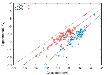
Figure 2: Calculated IPs using the LDA compared with experimental values. Blue stars show results from unconstrained minimization; red boxes show results of the constrained minimization. Red and blue lines are guides to the eye. The IP is found as the negative of the HOMO energy. The black dotted line corresponds to the ideal correlation between an exact calculation and experiment.

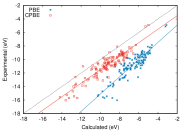
Figure 3: Calculated IPs using the PBE functional compared with experimental values. Blue stars show results from unconstrained minimization; red boxes show results of the constrained minimization. Red and blue lines are guides to the eye. The IP is found as the negative of the HOMO energy. The black dotted line corresponds to the ideal correlation between an exact calculation and experiment.

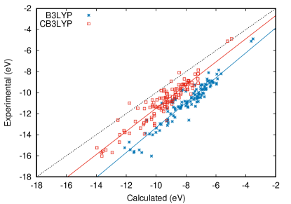
Figure 4: Calculated IPs using the B3LYP hybrid functional compared with experimental values. Blue stars show results from unconstrained minimization; red boxes show results of the constrained minimization. Red and blue lines are guides to the eye. The IP is found as the negative of the HOMO energy. The black dotted line corresponds to the ideal correlation between an exact calculation and experiment.

In Fig. 5, we plot the error in the calculated ionization potential $\Delta\textrm{IP}$, where this error is given by the difference between the experimental and calculated values, $\Delta\textrm{IP}=\textrm{IP}_{\textrm{exp}}-\textrm{IP}_{\textrm{calc}}$. A positive value in $\Delta\textrm{IP}$ implies an underestimation of the ionization potential. The inferior performance of the unconstrained relative to constrained minimization, is seen clearly in this figure, with IP errors of 4eV or more occurring frequently in the unconstrained case. The improvement of (unconstrained) B3LYP results over LDA and PBE is also evident, due to the partial cancellation of SIs in B3LYP. This improvement, however, is surpassed and offset by the constrained minimization technique to obtain the effective potential, with the three approximations giving similar results to each other.

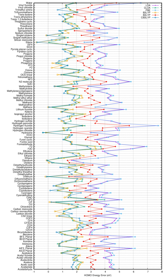
Figure 5: The differences between the calculated HOMO energy level and the experimental values for the ionization potential, comparing the unconstrained and constrained minimization of the LDA, PBE and B3LYP approximations. A positive value corresponds to an underestimation of the IP.

Table 1: The average error, $\bar{\Delta}$, standard deviation of the error, $\sigma$, average percentage error, $\bar{\delta}$, and standard deviation of the percentage error, $\bar{\sigma}$, from experimental results for the ionization potential (IP) for the molecules in Fig. 5. The IP was approximated by the energy of the HOMO calculated using unconstrained functionals LDA, PBE, B3LYP and the constrained functionals CLDA, CPBE, CB3LYP. The average energy increase, $\Delta E$, of the total energies of the constrained calculations compared to the unconstrained are also shown.

	LDA	CLDA	PBE	CPBE	B3LYP	CB3LYP
$\bar{\Delta}$ (eV)	4.08	1.61	4.20	1.51	2.94	1.42
$\sigma$ (eV)	0.93	0.74	0.94	0.77	0.71	0.73
$\bar{\delta}$	38%	15%	39%	14%	27%	13%
$\bar{\sigma}$	6%	6%	5%	7%	5%	6%
$\Delta E$ (meV)		0.1		0.2		0.3

A quantitative summary of the observations of the graphs in Figs. 2 - 5 can be found in Table 1. There, we show the average error, $\bar{\Delta}$, and the percentage error $\bar{\delta}$, defined by averaging over the absolute value of $\Delta\textrm{IP}$ from Fig. 5, and $|\Delta\textrm{IP}|/\textrm{IP}$. The standard deviations $\sigma$ and $\bar{\sigma}$ of the absolute values of the $\Delta\textrm{IP}$ and $|\Delta\textrm{IP}|/\textrm{IP}$ are also shown. The improvements of the constrained methods amount to a reduction in the average error for LDA and PBE by $\sim 2.5$eV while the B3LYP average error is halved to $\sim 1.5$eV. For LDA and PBE these reductions correspond to a percentage improvement of 25% and for B3LYP the improvement is 14% over the unconstrained result. The standard deviation of the constrained results are smaller than the unconstrained for LDA and PBE or almost equal for B3LYP. The quality of the results improves not only because the average error decreases but also the standard deviation.

An important result that is evident in Fig. 5 and Table 1 is the similarity of the results of the constrained optimizations, with all three approximations giving similar averages and similar deviations. One might expect this for the CLDA and CPBE calculations, since the unconstrained results are similar. However, although the B3LYP results are shifted by approximately 1eV compared to the LDA and PBE results, the CB3LYP results show no such shift when compared to CLDA and CPBE.

As far as total energies are concerned, the replacement of the KS potential with the constrained effective one is expected to raise the obtained total energies. In the last row of Table 1 we show the average increase in the total energy, $\Delta E$, from that of the corresponding KS calculation. We notice that the value of this increase is rather small. In other words, by enforcing the constraints of Eqs. (5), (6), we obtain total energies very close to the unconstrained KS minimum while on the other hand the orbital energies of the HOMO are substantially improved. As we have mentioned, the price is that the optimal potential is no longer the functional derivative of the potential energy with respect to the electron density. An interesting question of course is whether there exists a modified total energy functional that yields the obtained effective potential as its functional derivative w.r.t. the density. The almost negligible size of the total energy raise for the constrained calculation is consistent with the observationGritsenko et al. (2016) that potential terms with minimal influence in the total energy are responsible for the large deviation of the HOMO energies from the IPs. Thus, a viable path for correcting the HOMO energies is the identification and correction for such erroneous terms, as we aim to do in this work.

Another consequence of the constraint of Eq (5) is the introduction of a weak size inconsistency. Since the increase of the total energy for the constrained minimization has a very small value, the size inconsistency for the total energies is also minor. The effect on IPs on the other hand is more pronounced especially for small systems and goes to zero as the size of the constituent systems increases.

Calculations were also performed on a set of closed-shell anions where the IP coincides with the electron affinity (EA) of the neutral system. The advantages over unconstrained functionals can be clearly seen, these results are found in Table 2. Due to the expected diffuse nature of the HOMO in anions the augmented cc-pVTZ orbital basis set was used. With most approximate density functionals, the HOMO of the ions is found positive, i.e. they are predicted to have unbound electrons in most cases. This is a well known failure of many density functional approximations. With the constrained minimization method, we find that the same density functional approximations correctly predict that these anions have bound electrons, in agreement with experimental results. These results demonstrate that the improvements in the ionization energies are not limited to neutral molecules but can also be applied to anions.

Table 2: The calculated IPs (in eV) for a set of anions using both constrained and unconstrained methods for the functionals LDA, PBE, B3LYP compared with experimental values for the electron affinities of the neutral systems. The average error, $\bar{\Delta}$, the average percentage error, $\bar{\delta}$, and the average increase in the total energies, $\Delta E$, are shown for each of the functionals.

system	LDA	CLDA	PBE	CPBE	B3LYP	CB3LYP	Exp
CH${}_{3}^{-}$	-	0.30	-	0.26	-	0.51	0.08
CN-	0.17	2.96	0.05	2.78	1.33	3.45	3.86
Cl-	-	2.62	-	2.63	0.86	3.07	3.61
F-	-	2.24	-	2.16	0.01	2.62	3.40
NH${}_{2}^{-}$	-	0.23	-	0.15	-	0.50	0.77
OH-	-	1.07	-	0.98	-	1.42	1.83
PH${}_{2}^{-}$	-	0.74	-	0.75	-	0.91	1.27
SH-	-	1.57	-	1.57	-	1.91	2.31
SiH${}_{3}^{-}$	-	1.30	-	1.30	-	1.50	1.41
$\bar{\Delta}$ (eV)		0.66		0.70		0.41
$\bar{\delta}\>(^{*})$		35%		38%		20%
$\Delta E$ (meV)		0.015		0.052		0.15
(∗)The result for CH${}_{3}^{-}$ is excluded as it dominates the percentage error.

IV Conclusions

We have presented in detail and investigated the performance of the method by Gidopoulos and Lathiotakis Gidopoulos and Lathiotakis (2012a) to remove SI effects from the effective KS potential, for three popular DFAs, LDA, PBE, and B3LYP. A novelty of this method is the proposition that deficiencies of approximate KS potentials can be corrected by replacing the KS potentials with variationally optimized effective potentials that satisfy certain properties. In our method, these properties are that the electron repulsion density integrates to $N$-1 and is everywhere positive, Eqs. (5), (6).

The constrained minimization method was tested on its prediction for the ionization potential of a large set of molecules. Based on our results, the constrained method is found to offer substantial improvements for all approximate functionals tested, with a reduction of the average error for LDA from 4.08eV in the unconstrained case to 1.61eV with the constrained method. Similar reductions are found for PBE, while for the hybrid B3LYP functional the average error is almost halved from 2.94eV to 1.42eV. We also applied the method to the calculation of the HOMO energies of a group of anions which were found correctly negative. These energies, however, were found systematically smaller (by 20-38%) than the electron affinities of the neutral system. In addition, we found that, in all cases, the imposition of the constraints only marginally affects the total energy of the system. Finally, we point out that the corrected IPs obtained with our method are still not very accurate, reflecting the limitations of the underlying DFAs. Improved results for the IPs can be obtained either by a more refined DFA or by directly modeling the effective single particle potentialGritsenko et al. (1995); Schipper et al. (2000); Gritsenko et al. (2016).

These results show the importance of correcting for SI effects when calculating ionization potentials, and demonstrate the applicability of the constrained method in order to remove these self interaction effects in the KS potential. The constrained local potential is found to be a powerful method for improving the results of approximate functionals that contain self interactions.

Importantly, the constrained minimization results appear to be independent of the particular approximation, as can be seen from Fig. 5 and Table 1, where the constrained optimization results for the three DFAs give similar results. This property can be used to allow for more efficient calculations using a DFA that has a low computational cost but is of similar accuracy, once the constrained minimization method is used.

References

- Perdew and Zunger (1981) J. P. Perdew and A. Zunger, Physical Review B 23, 5048 (1981).
- Blair et al. (2015) A. I. Blair, A. Kroukis, and I. N. Gidopoulos, J Chem Phys 142, 084116 (2015).
- Lundberg and Siegbahn (2005) M. Lundberg and P. E. Siegbahn, The Journal of Chemical Physics 122, 224103 (2005).
- Rösch and Trickey (1997) N. Rösch and S. Trickey, The Journal of Chemical Physics 106, 8940 (1997).
- Toher et al. (2005) C. Toher, A. Filippetti, S. Sanvito, and K. Burke, Physical Review Letters 95, 146402 (2005).
- Goedecker and Umrigar (1997) S. Goedecker and C. Umrigar, Physical Review A 55, 1765 (1997).
- Perdew and Levy (1983) J. P. Perdew and M. Levy, Physical Review Letters 51, 1884 (1983).
- Almbladh and von Barth (1985) C.-O. Almbladh and U. von Barth, Phys Rev B 31, 3231 (1985).
- Görling (1999) A. Görling, Phys. Rev. Lett. 83, 5459 (1999).
- Gidopoulos and Lathiotakis (2012a) N. I. Gidopoulos and N. N. Lathiotakis, The Journal of chemical physics 136, 224109 (2012a).
- Gidopoulos and Lathiotakis (2015a) N. Gidopoulos and N. N. Lathiotakis, Advances In Atomic, Molecular, and Optical Physics 64, 129 (2015a), ISSN 1049-250X.
- van Leeuwen and Baerends (1994) R. van Leeuwen and E. J. Baerends, Phys. Rev. A 49, 2421 (1994).
- Legrand et al. (2002) C. Legrand, E. Suraud, and P.-G. Reinhard, Journal of Physics B: Atomic, Molecular and Optical Physics 35, 1115 (2002).
- Tsuneda and Hirao (2014) T. Tsuneda and K. Hirao, The Journal of chemical physics 140, 18A513 (2014).
- Pederson et al. (2014) M. R. Pederson, A. Ruzsinszky, and J. P. Perdew, The Journal of Chemical Physics 140, 121103 (2014).
- Gidopoulos and Lathiotakis (2015b) N. Gidopoulos and N. N. Lathiotakis, Advances In Atomic, Molecular, and Optical Physics 64, 129 (2015b), ISSN 1049-250X.
- Clark et al. (2017) S. J. Clark, T. W. Hollins, K. Refson, and N. I. Gidopoulos, J. Phys.: Condens. Matter 00, 8pp (2017).
- Kümmel and Perdew (2003) S. Kümmel and J. P. Perdew, Molecular Physics 101, 1363 (2003).
- Lathiotakis et al. (2014a) N. N. Lathiotakis, N. Helbig, A. Rubio, and N. I. Gidopoulos, Phys. Rev. A 90, 032511 (2014a).
- Lathiotakis et al. (2014b) N. N. Lathiotakis, N. Helbig, A. Rubio, and N. I. Gidopoulos, The Journal of Chemical Physics 141, 164120 (2014b).
- Theophilou et al. (2015) I. Theophilou, N. N. Lathiotakis, N. I. Gidopoulos, A. Rubio, and N. Helbig, The Journal of Chemical Physics 143, 054106 (2015).
- Perdew et al. (1996) J. P. Perdew, K. Burke, and M. Ernzerhof, Physical Review Letters 77, 3865 (1996).
- Becke (1993) A. D. Becke, The Journal of chemical physics 98, 5648 (1993).
- Lee et al. (1988) C. Lee, W. Yang, and R. G. Parr, Physical Review B 37, 785 (1988).
- Zhan et al. (2003) C.-G. Zhan, J. A. Nichols, and D. A. Dixon, The Journal of Physical Chemistry A 107, 4184 (2003).
- Hirata et al. (2001) S. Hirata, S. Ivanov, I. Grabowski, R. J. Bartlett, K. Burke, and J. D. Talman, J Chem Phys 115, 1635 (2001).
- Gidopoulos and Lathiotakis (2012b) N. I. Gidopoulos and N. N. Lathiotakis, Phys. Rev. A 85, 052508 (2012b).
- Lathiotakis and Marques (2008) N. Lathiotakis and M. A. Marques, The Journal of Chemical Physics 128, 184103 (2008).
- Johnson III (2011) R. D. Johnson III (2011), URL http://cccbdb.nist.gov.
- Zhang and Musgrave (2007) G. Zhang and C. B. Musgrave, The Journal of Physical Chemistry A 111, 1554 (2007).
- Gritsenko et al. (2016) O. V. Gritsenko, L. M. Mentel, and E. J. Baerends, The Journal of Chemical Physics 144, 204114 (2016).
- Gritsenko et al. (1995) O. Gritsenko, R. van Leeuwen, E. van Lenthe, and E. J. Baerends, Phys. Rev. A 51, 1944 (1995).
- Schipper et al. (2000) P. Schipper, O. Gritsenko, S. Van Gisbergen, and E. Baerends, The Journal of Chemical Physics 112, 1344 (2000).