Combining neural networks and signed particles to simulate quantum systems more efficiently,
Part II

Abstract

Recently the use of neural networks has been introduced in the context of the signed particle formulation of quantum mechanics to rapidly and reliably compute the Wigner kernel of any provided potential. This new technique has introduced two important advantages over the more standard finite difference/element methods: 1) it reduces the amount of memory required for the simulation of a quantum system. As a matter of fact, it does not require storing the kernel in a (expensive) multi-dimensional array, and 2) a consistent speedup is obtained since now one can compute the kernel on the cells of interest only, i.e. the cells occupied by signed particles. Although this certainly represents a step forward into the direction of rapid simulations of quantum systems, it comes at a price: the number of hidden neurons is constrained by design to be equal to the number of cells of the discretized real space. It is easy to see how this limitation can quickly become an issue when very fine meshes are necessary. In this work, we continue to ameliorate this previous approach by reducing the complexity of the neural network and, consequently, by introducing an additional speedup. More specifically, we propose a new network architecture which requires less neurons than the previous approach in its hidden layer. For validation purposes, we apply this novel technique to a well known simple, but very indicative, one-dimensional quantum system consisting of a Gaussian wave packet interacting with a potential barrier. In order to clearly show the validity of our suggested approach, time-dependent comparisons with the previous technique are presented. In spite of its simpler architecture, a good agreement is observed, thus representing one step further towards fast and reliable simulations of time-dependent quantum systems.

1 Introduction

In recent years, a new formulation of quantum mechanics has been introduced which does not rely on the standard concept of a wave function but, instead, is based on the new notion of an ensemble of particles provided with a sign. This novel approach is usually referred to as the signed particle formulation of quantum mechanics [1], while its numerical discretization is known as the Wigner Monte Carlo method. In spite of its relatively recent appearance, it has already been applied to the simulation of a plethora of different quantum systems, essentially for validation purposes during its development, in both the single- and many-body cases, showing unprecedent advantages in terms of computational resources [2]. For instance, it has allowed the time-dependent simulation of quantum many-body systems on relatively small machines in both the density functional theory (DFT) and first-principle frameworks [3], [4] for systems as complex as ensembles of indistinguishable Fermions [5]. Moreover, within this new approach, the inclusion of elastic and inelastic effects is trivial, see for instance [6] which describes a three-dimensional wave packet moving in a silicon substrate in the presence of a Coulomb potential at various temperatures with absorbing boundary conditions, a daunting task for other more standard and well known methods. The same approach has also been applied to the study of the resilience of entangled quantum systems in the presence of environmental noise [7]. To the best of the authors knowledge, this is the only formulation of quantum mechanics which can concretely tackle such problems by means of relatively affordable computational resources and without having to recur to arbitrary unphysical approximations.

Although this method has several unique features, the computation of the so-called Wigner kernel (essentially a multi-dimensional integral which is heavily utilized to predict the evolution of the particles) can quickly become a critical bottleneck for the simulation of quantum systems. In fact, both the amount of memory needed to store the kernel and the time for its computation are cursed by the total dimensionality of the system or, equivalently, by the dimensionality of the configuration space. Recently, an Artificial Neural Network (ANNs) has been presented to address the problem of computing the Wigner kernel rapidly and reliably by one of the authors of this work [8]. In this previous study, a new technique has been introduced which reduces both computational times and memory requirements. In more specific details, this relatively novel solution is based on the use of an appropriately tailored neural network which is exploited within the context of the signed particle formalism. The suggested neural network is able to compute accurately and rapidly the Wigner kernel and does not necessitate any training phase since all its weights and biases are specified by analytical formulas. Moreover, no relevant amount of memory is required for the kernel as it is now computed on the fly by the ANN only on the cells of the discretized phase-space which are occupied by particles (the reader is encouraged to read [8] for a complete list of details although a short summary is provided in the next section for the sake of consistency). Although this approach represents a step forward towards the simulation of time-dependent many-body quantum systems on affordable resources, therefore opening the way towards e.g. the effective design of quantum devices, it comes with an important constraint which can eventually represent a serious issue: the number of hidden neurons of the networks must be equal to the number of cells of the discretized configuration space. This can represent a serious drawback when fine meshes are utilized.

In this work, we further improve this technique by providing generalization capabilities to the network. This approach has the main advantage of reducing the complexity of the ANN and, therefore, allows a faster computation of the Wigner kernel itself. In more details, we propose a different ANN architecture which can work with a smaller number of hidden neurons, i.e. the constraint forcing them to be in the same number as the number of cells in the discretized configuration space is completely removed. For validation purposes, we apply this novel technique to a well-known simple, but very indicative, one-dimensional time-dependent system consisting of a Gaussian wave packet interacting with a potential barrier. In order to clearly show the validity of the approach, comparisons with our previously implemented, and validated, technique are presented.

This paper is organized as follows. In the next section, we start by introducing in some detail the previous technique which, for the first time, was able to combine the use of signed particles with an ANN. Then, we proceed with the description of the new approach which improves this particular method. Finally, a validation test is performed to assess the accuracy of the new suggested approach. Some conclusive comments are given afterwards. The authors believe this work opens the way towards different interesting directions such as, for instance, time-dependent quantum chemistry and design of quantum computing electronic devices, with incredible practical implications.

2 Signed Particles and Neural Networks

In this section, we start by discussing one postulate of the signed particle formulation which shows how to compute and use the Wigner kernel to evolve particles. Then, the technique previously implemented in [8] is described. This provides the context of our specific problem. Finally, we introduce our novel technique which simplifies the previous ANN approach while still keeping a good accuracy.

2.1 Signed particles and the Wigner kernel

The signed particle of quantum mechanics consists of a set of three rules or, equivalently postulates, which completely defines the time-dependent evolution of a quantum system. In this paragraph, we discuss one of these postulates, in particular postulate II, which can sometimes represent a serious bottleneck during the simulation of a system (see [1] and [2]). The other rules have been thoroughly presented and discussed elsewhere in the literature and can be summarized as 1) a quantum system is described by an ensemble of signed field-less classical particles which can be used to recover the corresponding Wigner quasi-distribution and, thus, its wave function, and 2) particles with opposite signs but equal position and momentum annihilate. Below, we introduce postulate II in full details in the context of a one-dimensional, single-body system (the generalization to many-dimensional, many-body systems is esily derived, see for example [2]).

Postulate. A signed particle, evolving in a given potential $V=V\left(x\right)$, behaves as a field-less classical point-particle which, during the time interval $dt$, creates a new pair of signed particles with a probability $\gamma\left(x(t)\right)dt$ where

$$\gamma\left(x\right)=\int_{-\infty}^{+\infty}\mathcal{D}p^{\prime}V_{W}^{+}\left(x;p^{\prime}\right)\equiv\lim_{\Delta p^{\prime}\rightarrow 0^{+}}\sum_{M=-\infty}^{+\infty}V_{W}^{+}\left(x;M\Delta p^{\prime}\right),$$ (1)

and $V_{W}^{+}\left(x;p\right)$ is the positive part of the quantity

$$V_{W}\left(x;p\right)=\frac{i}{\pi\hbar^{2}}\int_{-\infty}^{+\infty}dx^{\prime}e^{-\frac{2i}{\hbar}x^{\prime}\cdot p}\left[V\left(x+x^{\prime}\right)-V\left(x-x^{\prime}\right)\right],$$ (2)

known as the Wigner kernel (in a $d$-dimensional space) [9]. If, at the moment of creation, the parent particle has sign $s$, position $x$ and momentum $p$, the new particles are both located in $x$, have signs $+s$ and $-s$, and momenta $p+p^{\prime}$ and $p-p^{\prime}$ respectively, with $p^{\prime}$ chosen randomly according to the (normalized) probability $\frac{V_{W}^{+}\left(x;p\right)}{\gamma(x)}$.

Therefore, one can consider the signed particle formulation as constituted of two main parts: the evolution of field-less particles, which is always performed analytically, and the computation of the kernel (2), which is usually performed numerically. In particular, the computation of the Wigner kernel represents a formidable problem in terms of computational implementation. In fact, it is equivalent to a multi-dimensional integral which complexity increases exponentially with the dimensions of the configuration space (within both finite differences and Monte Carlo approaches). Moreover, the amount of required memory to perform such computations becomes rapidly daunting. Therefore, a naive approach to this particular task is neither appropriate nor affordable, even in the case where relevant computational resources are available (the reader interested in the technical details can find a free implementation of the signed particle formulation at [14]).

We now briefly describe our previous method recently discussed in [8] and then introduce our new technique.

2.2 A previous neural network approach

Recently, one of the authors of this work has suggested an ANN which, given a potential defined over the (discretized) configuration space, is capable of providing the Wigner kernel (2) with insignificant memory resources and at lower computational times, especially when compared to more standard integration methods. At a first glance, it might seem rather simple to train an ANN to predict the kernel function over the phase space, once a potential is provided (in other words, supervised learning). In fact, the problem simply consists in creating a map between a vector representing the potential and a matrix representing the kernel, a rather common problem in machine learning. It rapidly appears, though, that this naive approach based on a completely general ANN is not adapted to the complexity of the problem at hand and some prior knowledge must be exploited (interestingly enough, similar conclusions have been obtained in [10] and [11]). In particular, our previous analysis has shown that learning the Wigner-Weyl transform would require a relevant amount of data to be generated which, in turn, would require a very deep network due to the complexity of the problem at hand [12]. Although it is clearly desirable to have such a tool, our previous goal has been precisely to avoid this kind of difficulties. Surprisingly it has been shown, that by performing some relatively simple algebraic manipulation, an unexpected outcome emerges: it is actually possible to obtain such ANN without having to train it since we are in front of one rare example of neural network which weights can be computed analytically. In the following, we briefly describe this approach.

In the context of a one-body one-dimensional quantum system restricted to a finite domain, the Wigner kernel (2) can be expressed as:

$$V_{W}(x;p) = \frac{1}{i\hbar L_{C}}\int_{-\frac{L_{C}}{2}}^{\frac{L_{C}}{2}}dx^{\prime}\exp^{-2i\frac{xp}{\hbar}}$$ (3)

$$\times \left[V(x+x^{\prime})-V(x-x^{\prime})\right],$$

where the quantity $L_{C}$ defines the discretization of the momentum space, i.e. $\Delta p=\frac{\pi}{\hbar L_{C}}$. Now, by exploiting the fact that the Wigner kernel is a real function [9], and by taking into account the discreteness of the phase space [2] it becomes:

$$V_{W}(i;j) = \frac{-1}{\hbar L_{C}}\sum_{m=-\lfloor\frac{L_{C}}{2\Delta x}\rfloor}^{+\lfloor\frac{L_{C}}{2\Delta x}\rfloor}\sin\left(2\frac{(m\Delta xj\Delta p)}{\hbar}\right)$$ (4)

$$\times \left[V(i+m)-V(i-m)\right]\Delta x,$$

with $i=1,\cdots,n_{x}$, $j=-n_{p},\cdots,+n_{p}$, and $\lfloor X\rfloor$ being the integer part of the real number $X$.

By exploiting formula (4), and after some standard algebraic manipulation, it is possible to depict a neural network which computes the Wigner kernel (a one-to-one map between functions and neural networks exists which guarantees that our task is possible [13]) and Figure 1 shows its actual architecture. In particular, the network consists of an input layer, a hidden layer and an output layer. The input layer receives a discretized position in the phase space, indicated by the couple $(i,j)$, along with a corresponding discretized potential $V=V(x)$, represented by the vector $\left[V_{1}=V(x_{1}),\dots,V_{n}=V(x_{n})\right]$. To speed up the network, an initial pre-computation of the angles $\theta_{l}$ and the corresponding sinusoidals is performed. Afterwards, the potential and sinusoidal values are utilized to define the activation functions of the hidden layer and, eventually, an weighted average is computed in the last layer which represents the output of the network (see [8] for all details).

An interesting trait of this architecture is that the weights are determined analytically, in other words no training process is required (one finds that $w_{l}=-\frac{2\Delta x}{\hbar L_{C}}$, $\forall l$). Although not very common in the literature, this particular approach brings two important advantages. First, it completely avoids the need to compute the Wigner kernel everywhere on the (finite and discretized) phase-space (the function $V_{W}=V_{W}(x;p)$ can now be computed only where it is needed). Second, the curse of dimensionality affecting the other methods in terms of memory is completely removed from the picture. Despite these important features, one important drawback remains: the number of neurons in the hidden layer must equal the number of cells in the discretized configuration space. This means that the network still embeds the initial complexity of the problem.

2.3 A trained neural network approach

The objective of this section is the improvement of the previous approach by introducing an arbitrary number of parameters (in other words, weights) to be learnt. This adds generalization capabilities to the network which, in turn, allows the reduction of the number of calculations (i.e. less artificial neurons) necessary to (still reliably) compute the Wigner kernel. In order to achieve such goal, one starts from the previous approach and carefully modify it.

In particular, we start from the previous architecture and investigate ways to simplify and generalize it. If we consider the exact formula for the kernel (4), by grouping the terms by two and by exploiting the symmetry properties of a one-dimensional kernel with respect to the space of momenta, one obtains:

$$V_{W}(i,j) = \frac{-2\Delta x}{\hbar L_{C}}\sum_{m=0,\text{even}}^{\lfloor\frac{L_{C}}{2\Delta x}\rfloor}\left[V(2m)\times\sin{\left(\theta_{2m}(i,j)\right)}+V(2m+1)\times\sin{\left(\theta_{2m+1}(i,j)\right)}\right]$$

$$\approx \frac{-2\Delta x}{\hbar L_{C}}\sum_{m=0,\text{even}}^{\lfloor\frac{L_{C}}{2\Delta x}\rfloor}\left(\frac{V(2m)+V(2m+1)}{2}\right)\left[\sin{\left(\theta_{2m}(i,j)\right)}+\sin{\left(\theta_{2m+1}(i,j)\right)}\right]$$

$$= \frac{-2\Delta x}{\hbar L_{C}}\cos{\left(\frac{j\Delta p\Delta x}{\hbar}\right)}\sum_{m=0,\text{even}}^{\lfloor\frac{L_{C}}{2\Delta x}\rfloor}\left[V(2m)+V(2m+1)\right]$$

$$\times \sin{\left(\frac{\theta_{2m}(i,j)+\theta_{2m+1}(i,j)}{2}\right)}$$

where the angle $\theta_{l}(i,j)=2\frac{(l-i)\Delta xj\Delta p}{\hbar}$ and the assumption of low variations of the potential $V=V(x)$ over neighbor cells of a finely enough discretized phase space is introduced (which represents a reasonable hypothesis in computational physics), represented by the cell lenghts $\Delta x$ and $\Delta p$, i.e.

$$V(i)\approx V(i+1)\approx\frac{V(i)+V(i+1)}{2}.$$

The assumption above (essentially a baricentric interpolation), although arbitrary and dependent on the discretization lenght $\Delta x$, offers a first simple way to improve the approach described in the previous section [8].

Clearly, other interpolation schemes might be utilized which could lead to better approximations of the kernel $V_{W}=V_{W}(x;p)$. For instance, one might wonder if a weighted average of the angles in the sinusoidal functions might offer some further advantage in terms of generalization and, therefore, numerical performance. Moreover, it would be of great help if the best interpolation could be extracted automatically. Therefore, we consider the following more general expression for the kernel, which consists in regrouping $N$ terms of the original exact sum in (4):

$$V_{W}(i,j)=\prod_{s=0}^{m-1}\cos{\left(\frac{2^{s}j\Delta p\Delta x}{\hbar}\right)}\sum_{l=0}^{n/N-1}W_{l}(\sum_{p=1}^{N}\omega_{p}^{V}V_{Nl+p})\sin\left(\sum_{p=1}^{N}\omega_{p}^{\theta}\theta_{Nl+p}(i,j)\right)$$ (5)

which can be implemented in the shape of a trainable neural network like the one depicted in Fig. 2 (further details are provided in the next section), for some integers $N$ and $n$ representing the number of potential values utilized at one neuronal site and the number of hidden neurons respectively, and where the parameters $(\omega_{1}^{\theta},\omega_{2}^{\theta},...,\omega_{N}^{\theta})$, along with the parameters $(\omega_{1}^{V},\omega_{2}^{V},...,\omega_{N}^{V})$ and, finally, the parameters $(W_{1},...,W_{n/N})$ represent the weights of the network which need to be trained. In order to find those values, we search for the weights which provide the best network approximation of the function $V_{W}=V_{W}(x;p)$ (representing the dataset) by means of a standard machine learning method known as stochastic gradient descent. The details of the numerical experiments performed in this work are discussed in the next section.

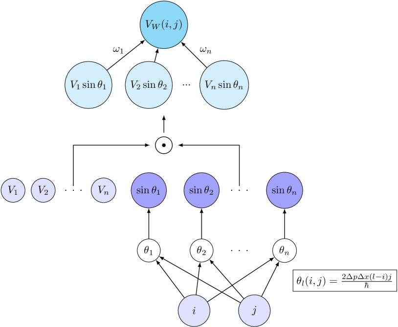
Figure 1: Neural network corresponding to formula (4). This architecture network consists of an input layer, a hidden layer and an output layer. The input layer receives a discretized position in the phase space, indicated by the couple $(i,j)$, and a corresponding discretized potential $V=V(x)$, represented by the vector $\left[V_{1}=V(x_{1}),\dots,V_{n}=V(x_{n})\right]$. An initial pre-processing phase is performed, consisting of the angles $\theta_{i}$ and the corresponding sinusoidals. Then, the potential and sinusoidal values are utilized to define the activation functions of the hidden layer and, eventually, an weighted average is computed in the output layer (see [8] for all details).

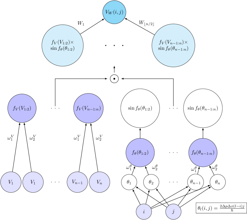
Figure 2: Neural network corresponding to formula (5). This architecture network consists of an input layer, two hidden layers and an output layer. Exactly as for the ANN presented in Fig. 1, the input layer receives a discretized position in the phase space, indicated by the couple $(i,j)$, and a discretized potential $V=V(x)$, represented by the vector $\left[V_{1}=V(x_{1}),\dots,V_{n}=V(x_{n})\right]$. As usual, the angles $\theta_{i}$ are pre-computed along with the functions $f_{\theta}$ and $f_{V}$. This network is trained by means of a common method of machine learning, stochastic gradient descent, until the weights which minimize the loss function (MSE) are found (see Fig. 3 below).

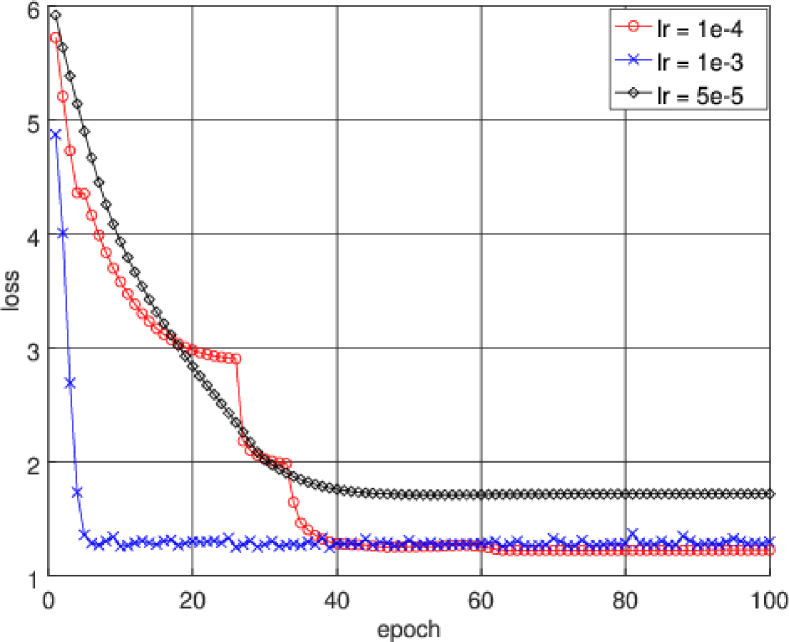
Figure 3: Convergence curves on the training set of the neural network corresponding to formula (5) with $N=2$ and represented in Fig. 2. The method utilized is the stochastic gradient descent. The ANN was trained using various hyper-parameters, respectively $10^{-3}$ (blue crosses), $10^{-4}$ (red circles) and $10^{-5}$ (black diamonds). One observes that a learning rate equal to $10^{-4}$ provides the best convergence.

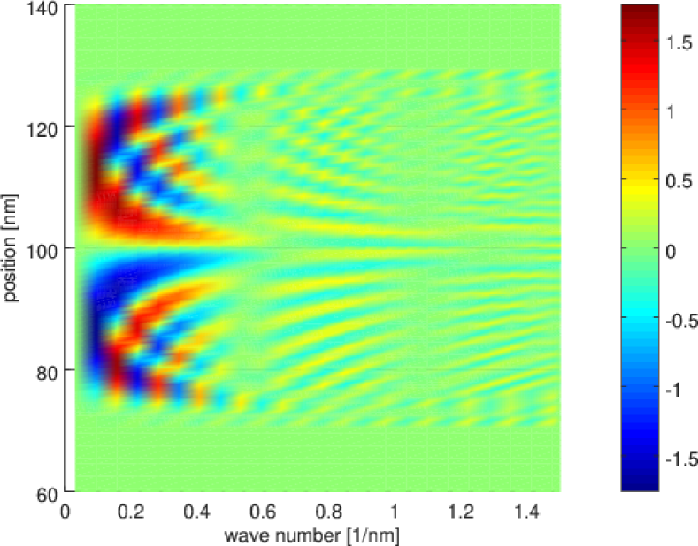
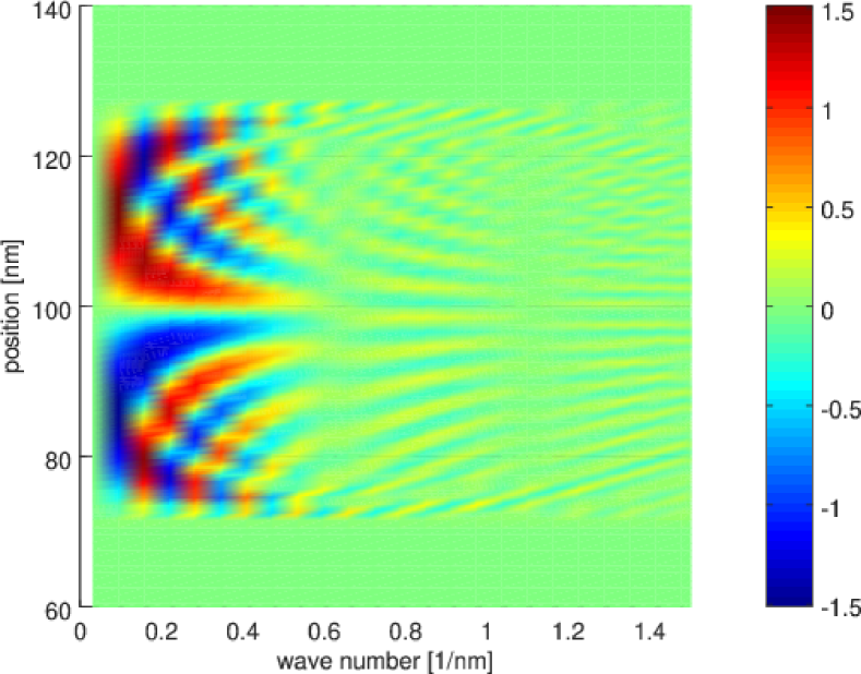
Figure 4: Wigner kernels for the cases $N=1$ (top) and $N=2$ (bottom) respectively. A good agreement is found: the shapes of the two kernels are pratically identical, along with their numerical values (only a small difference can be found on the maxima and minima as shown in the color bars). Their difference is represented in Fig.5.

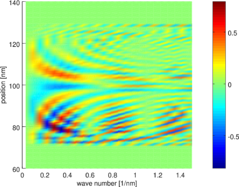
Figure 5: Difference between the kernels corresponding to the case $N=1$ and $N=2$ as shown in Fig.4.

3 Numerical validation

In this section, we propose and discuss a test which aim is to show the validity of our suggested new approach. To that purpose, we simulate an archetypal quantum system consisting of a one-dimensional Gaussian wave packet moving against a potential barrier positioned at the center of a finite domain ($200$nm), with width and height equal to $6$nm and $-0.3$eV respectively, and with the following initial conditions:

$$f^{0}_{W}(x;M)=Ne^{-\frac{(x-x_{0})^{2}}{\sigma^{2}}}e^{-\frac{1}{\hbar^{2}}(M\Delta p-p_{0})^{2}\sigma^{2}}$$ (6)

with $N$, $p_{0}$, $x_{0}$ and $\sigma$ the constant of normalization. The initial position, dispersion and wave number of the packet are equal to $68.5$nm, $10$nm and $6.28\cdot 10^{-2}$nm^-1 respectively. This corresponds to an initial energy of the wave packet smaller than the energy of the barrier. Therefore, one expects both reflection and tunneling effects happening during the time-dependent evolution of the system. Finally, absorbing boundary conditions are applied at the edge of the simulation domain. This numerical experiment, in spite of its simplicity, represents a well founded validation test. Although more complex situations could be simulated, it would be out of the scope of this work.

Even if many options are available, for the sake of clarity and simplicity, we focus on a neural network (5) with $N=2$ (the reader should note that the case $N=1$ corresponds to our previous approach) and depicted in Fig. 2 with the functions $f_{\theta}$ and $f_{V}$ are hereby introduced for convenience and defined as:

$$f_{\theta}(\theta_{kN+1:(k+1)N}) = \sum_{p=1}^{N}\omega_{p}^{\theta}\theta_{kN+p},$$

$$f_{V}(V_{kN+1:(k+1)N}) = \sum_{p=1}^{N}\omega_{p}^{V}V_{kN+p},$$

(these functions may be considered as one-dimensional convolutions over the potentials $V_{l}$ and the angles $\theta_{l}$ respectively), with $\theta_{kN+1:(k+1)N}$ and $V_{kN+1:(k+1)N}$ being vectors of angles and potentials, respectively, with indices ranging from $kN+1$ to $(k+1)N$. Thus, the suggested network consists of an input layer, two hidden layers, and an output layer. In particular, this corresponds to an ANN with a number of neurons in the hidden layer (with sinusoidal activation functions) which is exactly half times the number of hidden neurons of our previously proposed architecture [8]. This corresponds to a quite significant speedup since previously we had to evaluate two times more sinusoidal functions (which are well known to be very expensive functions in terms of computational time).

In order to train such an ANN, examples of potentials and their corresponding Wigner kernels have been created which simply consist of a series of Gaussian bell shaped potentials with different randomly chosen central positions, heights and dispersions. Therefore, the data set consists of a series of vectors embedding two integers $(i,j)$ defining the position in the phase space at which the kernel must evaluated and the (discretized) potential itself $(V_{1},\dots,V_{n})$, to which the corresponding values of the corresponding kernel $V_{W}(i;j)$ are attached, in other words, it represents a regression problem (the kernels are computed by finite difference schemes). By minimizing a standard mean squared error (MSE) loss function, we found that at most a hundred examples were necessary to achieve a meaningful convergence during the training process, in less than $200$ epochs. On a final but interesting note, by numerical experimentation, it is possible to observe that the choice of $N$ represents a trade-off between efficiency and the accuracy of the solution. In fact, the larger the number $N$ is and the faster the computation of the kernel is, but at the price of a lower accuracy. This is why we focus only on the case $N=2$ in this work (further investigation will be performed in the next future since this seems to be a promising direction). We trained our model with various hyper-parameters, more specifically learning rates, as it is shown in Fig. 3 which represents the error on the training data set. Eventually, we observe that a learning rate equal to $10^{-4}$ provides the best convergence. Thus, this network is utilized to compute the kernel of a given potential during the simulation of a quantum system by means of signed particles. The results of our numerical experiment are reported in Figs. 4 - 7.

In particular, Fig.4 shows the Wigner kernels obtained with the neural network in Fig.2 for the cases $N=1$ (top) and $N=2$ (bottom). The shapes of the two kernels, in spite of the very different methods utilized to compute them (and their different degrees of accuracy), are pratically identical and their numerical values are very close (a small difference can be found on the color bars). Since it is difficult to spot any difference by the naked eye, their mathematical difference is shown in Fig.5. Although some value seem pretty high, one should note that they are very localized in the phase space. Due to the stochastic nature of the evolution of signed particles, one quickly realizes that the introduction of localized noise into the kernels (due, e.g., to some lack of accuracy) should not greatly affect the time-dependent evolution of the whole system. This should not come as a surprise as it is well known that such advatange is typical of stochastic approaches. Finally, the time-dependent evolution of the wave packet for the cases $N=1$ and $N=2$ is reported in Fig.7 at times $1$fs, $2$fs, $3$fs and $4$fs respectively. A very good agreement is found between the two methods, clearly showing the validity of our novel approach.

Figure 6: Comparison between the gamma functions corresponding to the cases $N=1$ (red circles) and $N=2$ (blue crosses). A very good agreement between the two functions is clearly visible.

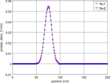
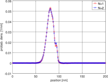
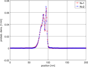
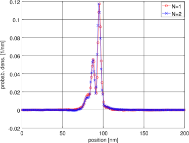
Figure 7: Time-dependent evolution of a wave packet interacting with a potential barrier positioned at the center of the spatial domain, at times $1$fs (top left), $2$fs (top right), $3$fs (bottom left) and $4$fs (bottom right) respectively, and with two different kernels corresponding to the cases $N=1$ (red circles) and $N=2$ (blue crosses).

4 Conclusions

In this work, we introduced a new technique which combines neural networks and the signed particle formulation of quantum mechanics to achieve fast and reliable time-dependent simulations of quantum systems. It can be considered as an improvement and generalization of the technique recently suggested in [8]. In practice, the method consists of two steps. First, the Wigner kernel corresponding to a given potential is computed by means of a neural network which has previously been trained to perform the transformation described in formula (2). Then, the evolution of the signed particles is performed as usual [1], [2]. One of the feature of the neural network suggested in this work is generalization capabilities. Therefore, it now achieves a further important speedup when compared to our previous method which needs more units in its hidden layer (specifically, two times more sinusoidal activation functions). A representative validation test consisting of a wave packet impinging on a potential barrier has been performed which clearly shows that, although the approach discussed in this work utilizes computational resources, it is still accurate, reliable and suitable for practical tasks.

As we are approaching the era of quantum technologies (e.g. quantum computing, quantum chemistry, nanotechnologies, etc), our quantum simulation and design capabilities are now starting to play a fundamental role which is going to keep growing in importance in the future. In this new and exciting context, solving modern technological problems is going to imply adopting modern and (possibly dramatically) different approaches to quantum mechanics. The authors of this paper believe that their suggested approach is a promising candidate from this perspective.

Acknowledgments. One of the authors, JMS, would like to thank M. Anti and T. Bollinger for their support, ethusiasm and encouragement.

References

- [1] J.M. Sellier, A Signed Particle Formulation of Non-Relativistic Quantum Mechanics, Journal of Computational Physics 297, pp. 254-265, (2015).
- [2] J.M. Sellier, M. Nedjalkov, I. Dimov, An Introduction to the Applied Quantum Mechanics in the Wigner Monte Carlo Formalism, Physics Reports 577, pp. 1-34, (2015).
- [3] J.M. Sellier, I. Dimov, A Wigner Monte Carlo Approach to Density Functional Theory, Journal of Computational Physics 270, pp. 265-277, (2014).
- [4] J.M. Sellier, I. Dimov, The Many-body Wigner Monte Carlo Method for Time-dependent Ab-initio Quantum Simulations, Journal of Computational Physics 273, pp. 589-597, (2014).
- [5] J.M. Sellier, I. Dimov, On the Simulation of Indistinguishable Fermions in the Many-Body Wigner Formalism, Journal of Computational Physics 280, pp. 287-294, (2015).
- [6] J.M. Sellier, I. Dimov, The Wigner-Boltzmann Monte Carlo method applied to electron transport in the presence of a single dopant, Computer Physics Communications 185, pp. 2427-2435, (2014).
- [7] J.M. Sellier, K.G. Kapanova, A Study of Entangled Systems in the Many-Body Signed Particle Formulation of Quantum Mechanics, International journal of quantum chemistry, 10.1002/qua.25447, (2017).
- [8] J.M. Sellier, Combining Neural Networks and Signed Particles to Simulate Quantum Systems More Efficiently, Physica A 496, pp. 62-71, (2018).
- [9] E. Wigner, On the quantum correction for thermodynamic equilibrium, Physical Review 40, no. 5, 749, (1932).
- [10] G. Carleo, Ma. Troyer, Solving the Quantum Many-body Problem with Artificial Neural Metworks, Science 355, pp. 602–606, (2017).
- [11] F. Brockherde, L. Vogt, L. Li, M. E. Tuckerman, K. Burke, K.-R. Muller, Bypassing the Kohn-Sham Equations with Machine Learning, Nature Communications, vol. 8, 872, (2017).
- [12] I. Goodfellow, Y. Bengio, A. Courville, Deep Learning, The MIT Press, (2016).
- [13] C.M. Bishop, Neural Networks for Pattern Recognition, Oxford University Press, (1995).
-
[14]
J.M. Sellier, nano-archimedes, accessed 24 May 2018,
URL: www.nano-archimedes.com