Open and closed random walks with fixed edgelengths in $\mathbb{R}^{d}$

Abstract

In this paper, we consider fixed edgelength $n$-step random walks in $\mathbb{R}^{d}$. We give an explicit construction for the closest closed equilateral random walk to almost any open equilateral random walk based on the geometric median, providing a natural map from open polygons to closed polygons of the same edgelength. Using this, we first prove that a natural reconfiguration distance to closure converges in distribution to a Nakagami$(\nicefrac{{d}}{{2}},\nicefrac{{d}}{{d-1}})$ random variable as $n\rightarrow\infty$. We then strengthen this to an explicit probabilistic bound on the distance to closure for a random $n$-gon in any dimension with any collection of fixed edgelengths $w_{i}$. Numerical evidence supports the conjecture that our closure map pushes forward the natural probability measure on open polygons to something very close to the natural probability measure on closed polygons; if this is so, we can draw some conclusions about the frequency of local knots in closed polygons of fixed edgelength.

I Introduction

Random walks in space with fixed edgelengths have been of interest to statistical physicists and chemists since Lord Rayleigh’s day. These walks model polymers in solution (at least under $\theta$-solvent conditions) [Rayleigh:1919do, hughes1995random, FloryPaulJ1969Smoc] and are similarly interesting in computational geometry and mathematics as a space of “linkages” [Demaine:2007jh, MR2004a:14059]. While 2- and 3-dimensional walks are the most relevant to this case, high-dimensional random walks often shed light on the lower dimensional situation [Rudnick:1987jn].

In this paper, we will consider the relationship between open and closed random walks of fixed edgelengths. We will provide an explicit algorithm for finding the nearest closed polygon with given edgelengths to almost any collection of edge directions, and use our construction to provide tail bounds on the fraction of polygon space within a fixed distance of the closed polygons in any dimension. Our results will be strongest for equilateral polygons, but provide explicit bounds for any collection of edgelengths.

To establish notation, we describe random walks in $\mathbb{R}^{d}$ with (fixed) positive edgelengths $w_{i}$ by their edge clouds $(w_{1},\hat{x}_{1}),\ldots,(w_{n},\hat{x}_{n})$ where $\hat{x}_{i}\in S^{d-1}$ is the direction of the $i$th edge. The space of polygonal arms $\operatorname{Arm}(n,d,w)$ is topologically equivalent to $(S^{d-1})^{n}$. If we let $\omega_{i}=\frac{w_{i}}{\sum w_{i}}$ be the relative edgelengths, then we can define the submanifold $\{\boldsymbol{x}:\sum\omega_{i}\hat{x}_{i}=\vec{0}\}$ of closed polygons $\operatorname{Pol}(n,d,w)$.

Using Bernstein’s inequality (e.g. [Dubhashi:2009ho]), there is an easy concentration inequality which suggests that the endpoints of random arms are close together. For equilateral polygons in $\mathbb{R}^{3}$, this takes the simple form

Theorem 1.

If $\boldsymbol{x}$ is chosen randomly in $\operatorname{Arm}(n,3,1)$ with edges $\hat{x}_{1},\ldots,\hat{x}_{n}$,

$$\mathcal{P}\left(\frac{1}{n}\left\|\sum\hat{x}_{i}\right\|<t\right)\geq 1-3\,e^{-nt^{2}\cdot\frac{3}{6+2\sqrt{3}t}}.$$

That is, the center of mass of a random edge cloud is very likely to be close to the origin. We can clearly close a random polygon in $\operatorname{Arm}(n,3,1)$ by subtracting the (small) $\frac{1}{n}\sum\hat{x}_{i}$ from each edge. That closed polygon is clearly near the original arm, but it is no longer equilateral. This raises the question of whether we can generally close a polygon in $\operatorname{Arm}(n,3,1)$ (or $\operatorname{Arm}(n,d,w)$) while preserving edgelengths and changing the polygon only a small amount. This question is the focus of this paper.

Given $\boldsymbol{x}$ and $\boldsymbol{y}$ in $\operatorname{Arm}(n,d,w)$, we view both as vectors in $\mathbb{R}^{dn}$ and measure the distance between them accordingly. We call this the chordal distance because it does not measure the arc on the spheres of radius $w_{i}$ for each pair of edges, but rather measures the straight line distance between edge vectors.

Our first main result is Proposition 10, which shows that the chordal distance between a random $\boldsymbol{x}\in\operatorname{Arm}(n,d,1)$ and the nearest $\boldsymbol{y}\in\operatorname{Pol}(n,d,1)$ converges in distribution to a Nakagami-$(\nicefrac{{d}}{{2}},\nicefrac{{d}}{{d-1}})$ random variable with PDF proportional to $x^{d-1}e^{-\frac{d-1}{2}x^{2}}$ as $n\rightarrow\infty$.

Our second main result is a general probabilistic bound on the chordal distance to closure for random polygons in any $\operatorname{Arm}(n,d,w)$. For equilateral polygons in $\mathbb{R}^{3}$, our main theorem (Corollary LABEL:cor:chordal_concentration) takes the very simple form

$$\mathcal{P}\left(d_{\text{chordal}}(\boldsymbol{x},\operatorname{Pol}(n,3,1))<t\right)\geq 1-6\exp\left(\nicefrac{{-t^{2}}}{{4}}\right)$$

for $t<\frac{\sqrt{n}}{200\sqrt{2}}$.

Here is a broad overview of our arguments. Given a polygon $\boldsymbol{x}$ in $\operatorname{Arm}(n,d,w)$, we will provide an explicit construction for a nearby closed polygon in $\operatorname{Pol}(n,d,w)$, which we call the geometric median closure of $\boldsymbol{x}$ (denoted $\operatorname{gmc}(\boldsymbol{x})$). It will be clear how to construct the geodesic in $\operatorname{Arm}(n,d,w)$ from $\boldsymbol{x}$ to $\operatorname{gmc}(\boldsymbol{x})$. For equilateral polygons, we show $\operatorname{gmc}(\boldsymbol{x})$ is the closest closed polygon to $\boldsymbol{x}$ in chordal distance (Theorem 8).

The distance between $\boldsymbol{x}$ and $\operatorname{gmc}(\boldsymbol{x})$ depends on the norm $\|\vec{\mu}\|$ of the geometric median (or Fermat-Weber point) of the edge cloud (Proposition 12). For equilateral polygons, we will be able to leverage existing results of Niemiro [Niemiro:1992ez] to find the asymptotic distribution of the geometric median of a random point cloud (Proposition 9). Combining this with the matrix Chernoff inequalities proves our first main result (Proposition 10).

The second main result follows from a concentration inequality for a random polygon in any $\operatorname{Arm}(n,d,w)$, which bounds the probability of a large $\|\vec{\mu}\|$ in terms of $n$, $d$, and $w$. This concentration result (Theorem 18) follows from parallel uses of the scalar and matrix Bernstein inequalities to control the expected properties of a random edge cloud, together with the definition of the geometric median as the minimum of a convex function.

Last, we will observe that the pushforward measure on closed polygons obtained by closing random open polygons appears to converge rapidly to the uniform distribution on closed polygons (Conjecture LABEL:conj:pushforward). Since these closures involve only very small motions of any part of the polygon, local features (such as small knots) should be preserved – it would follow (Conjecture LABEL:conj:local_knotting) that the rate of production of local knots in open and closed arcs should be almost the same.

II Constructing a nearby closed polygon

As mentioned above, we view $n$-edge polygons (up to translation) in $\mathbb{R}^{d}$ as collections of edge vectors $\vec{x}_{i}\in\mathbb{R}^{d}$. The vertices are obtained by summing the $\vec{x}_{i}$ from an arbitrary basepoint. In this section of the paper, we will assume only that the lengths of the edges of the polygon are fixed to some arbitrary $w_{i}=\|\vec{x}_{i}\|$. We will think of these fixed edgelength polygons in two ways:

• as a weighted point cloud on the unit sphere $S^{d-1}\subset\mathbb{R}^{d}$ where the points are denoted $\hat{x}_{i}=\vec{x}_{i}/\|\vec{x}_{i}\|$ and the weights are the $w_{i}$. We will call $(w_{i},\hat{x}_{i})$ the edge cloud of the polygon.

• as a point $\boldsymbol{x}\in\prod S^{d-1}(w_{i})\subset(\mathbb{R}^{d})^{n}=\mathbb{R}^{dn}$ (where $S^{d-1}(r)$ is the sphere of radius $r$). We will call $\boldsymbol{x}$ the vector of edges of the polygon.

The space of these polygons will be denoted $\operatorname{Arm}(n,d,w)=\prod S^{d-1}(w_{i})$. Within this space, there is a submanifold $\operatorname{Pol}(n,d,w)$ of closed polygons defined by the condition $\sum w_{i}\hat{x}_{i}=\vec{0}$. (Equivalently, $\boldsymbol{x}$ is closed if it lies in the codimension $d$ subspace of $\mathbb{R}^{dn}$ normal to the $\boldsymbol{n}^{j}=(\hat{e}_{j},\ldots,\hat{e}_{j})$, where $\hat{e}_{1},\ldots,\hat{e}_{d}$ is the standard basis in $\mathbb{R}^{d}$.) Both $\operatorname{Arm}(n,d,w)$ and $\operatorname{Pol}(n,d,w)$ are Riemannian manifolds with standard metrics, but it will be useful to use two additional metrics as well:

Definition 2.

The chordal metric on $\operatorname{Arm}(n,d,w)$ is given by

$$d_{\text{chordal}}(\boldsymbol{x},\boldsymbol{y})=\|\boldsymbol{x}-\boldsymbol{y}\|_{\mathbb{R}^{dn}}=\left(\sum\|w_{i}\hat{x}_{i}-w_{i}\hat{y}_{i}\|_{\mathbb{R}^{d}}^{2}\right)^{\nicefrac{{1}}{{2}}}.$$

The max-angular metric on $\operatorname{Arm}(n,d,w)$ is given by

$$d_{\text{max-angular}}(\boldsymbol{x},\boldsymbol{y})=\max_{i}\angle(\vec{x}_{i},\vec{y}_{i}).$$

We now make an important definition:

Definition 3.

A geometric median (also known as a Fermat-Weber point) of an edge cloud $(w_{i},\hat{x}_{i})$ is any point $\vec{\mu}$ which minimizes the weighted average distance function $\operatorname{Ad}_{\boldsymbol{x}}(\vec{y})$ given by

$$\operatorname{Ad}_{\boldsymbol{x}}(\vec{y})=\sum_{i}\omega_{i}\|\hat{x}_{i}-\vec{y}\|.$$

where $\omega_{i}=\nicefrac{{w_{i}}}{{\sum w_{i}}}$. To clarify notation, we will only use $\vec{\mu}$ for points which are a geometric median of a weighted point cloud; the point cloud will be clear from the context.

This is a very old construction with a beautiful theory around it; see the nice review in [Hamacher:2002vp]. We note that the geometric median differs from the center of mass (or geometric mean) of the points, which minimizes the weighted average of the squared distances between $\vec{y}$ and the $\hat{x}_{i}$ and that the geometric median is unique unless the points are all colinear and the geometric median is not one of the points.

This section is devoted to analyzing the following construction:

Definition 4.

Suppose $\boldsymbol{x}$ is a polygon and $\vec{\mu}$ is a geometric median of its edge cloud $(w_{i},\hat{x}_{i})$ which is not one of the $\hat{x}_{i}$. The geometric median closure $\operatorname{gmc}(\boldsymbol{x})$ of $\boldsymbol{x}$ is the polygon whose edge cloud has the same weights and edge directions obtained by recentering the $\hat{x}_{i}$ on $\vec{\mu}$ and renormalizing: $\operatorname{gmc}(\boldsymbol{x})$ has edge cloud $\left(w_{i},\frac{\hat{x}_{i}-\vec{\mu}}{\left|\hat{x}_{i}-\vec{\mu}\right|}\right)$.

If every geometric median of $(w_{i},\hat{x}_{i})$ is one of the $\hat{x}_{i}$, $\operatorname{gmc}(\boldsymbol{x})$ is not defined. If $\operatorname{gmc}(\boldsymbol{x})$ is defined, we say that $\boldsymbol{x}$ is median-closeable.

Of course, we need to justify our choice of name by proving that $\operatorname{gmc}(\boldsymbol{x})$ is closed. The key observation is the following Lemma, which follows by direct computation:

Lemma 5.

The function $\operatorname{Ad}_{\boldsymbol{x}}(\vec{y})$ is a convex function of $\vec{y}$. The gradient is given by

$$\nabla\!\operatorname{Ad}_{\boldsymbol{x}}(\vec{y})=\sum\omega_{i}\frac{\vec{y}-\hat{x}_{i}}{\|\vec{y}-\hat{x}_{i}\|}.$$

The Hessian of $\operatorname{Ad}_{\boldsymbol{x}}(\vec{y})$ is given by

$$\mathcal{H}\operatorname{Ad}_{\boldsymbol{x}}(\vec{y})=\left(\sum_{i}\frac{\omega_{i}}{\left\|\hat{x}_{i}-\vec{y}\right\|}\right)I_{d}-\left(\sum_{i}\frac{\omega_{i}}{\left\|\hat{x}_{i}-\vec{y}\right\|^{3}}(\vec{y}-\hat{x}_{i})(\vec{y}-\hat{x}_{i})^{T}\right).$$

Proposition 6.

If $\boldsymbol{x}$ is median-closeable, $\operatorname{gmc}(\boldsymbol{x})$ is a unique closed polygon with edgelengths $w_{i}$.

Proof.

The proof follows from assembling several standard facts about the geometric median. These are in [Anonymous:1UuVxm-1], but are easily checked by hand.

As it is a sum of convex functions, the average distance function $\operatorname{Ad}_{\boldsymbol{x}}$ is convex. Away from the $\hat{x}_{i}$, it is differentiable. If the points $\hat{x}_{i}$ are not colinear, $\operatorname{Ad}_{\boldsymbol{x}}$ is strictly convex and $\vec{\mu}$ is unique. If the points $\hat{x}_{i}$ are colinear, either the geometric median is one of the $\hat{x}_{i}$ or the set of geometric medians consists of the interval between two $\hat{x}_{i}$.

Any geometric median which is not one of the $\hat{x}_{i}$ must be a critical point of the average distance function. For any such $\vec{\mu}$, using Lemma 5,

$$\sum_{i}w_{i}\frac{\hat{x}_{i}-\vec{\mu}}{\left|\hat{x}_{i}-\vec{\mu}\right|}=-\left(\sum w_{i}\right)\nabla\!\operatorname{Ad}_{\boldsymbol{x}}(\vec{\mu})=0.\marginpar{\raggedright\tiny\ref{eq:grad total distance}eq:gradtotaldistance}\ignorespaces\@add@raggedright$$ (1)

This implies that $\operatorname{gmc}(\boldsymbol{x})$ is closed.

If $\vec{\mu}$ is unique, then $\operatorname{gmc}(\boldsymbol{x})$ is obviously unique. If $\vec{\mu}$ is not unique, the $\hat{x}_{i}$ are colinear, and $\vec{\mu}$ is on the line segment between two of the $\hat{x}_{i}$. In this case, it is not hard to see that (1) implies that the edges of $\operatorname{gmc}(\boldsymbol{x})$ are two antipodal groups of points on $S^{k-1}$, each containing $n/2$ points, regardless of where we take $\vec{\mu}$ on the segment. ∎

Our next goal is to prove an optimality property for the geometric median closure. We will start by proving a more general fact about recentering and renormalizing:

Proposition 7.

Suppose that $\hat{x}_{i}$ is any point cloud in $(S^{d-1})^{n}$, and $\vec{p}\in\mathbb{R}^{d}$ is not one of the $\hat{x}_{i}$. Given any set of weights $w_{i}$, we let $r(\boldsymbol{x};\vec{p},w)$ denote the renormalized, recentered, and reweighted point cloud, and $\vec{s}$ denote its weighted sum:

$$r(\boldsymbol{x};\vec{p},w):=\left(w_{i},\frac{\hat{x}_{i}-\vec{p}}{\left|\hat{x}_{i}-\vec{p}\right|}\right)\quad\text{and}\quad\vec{s}:=\sum_{i}w_{i}\frac{\hat{x}_{i}-\vec{p}}{\left|\hat{x}_{i}-\vec{p}\right|}.$$

If $\boldsymbol{x}=(\hat{x}_{1},\ldots,\hat{x}_{n})$ and $\boldsymbol{r}$ is the vector of edges corresponding to the edge cloud $(w_{i},\hat{r}_{i})$, then

$$\boldsymbol{r}=\operatorname{argmin}_{\sum w_{i}\hat{y}_{i}=\vec{s}}\|\boldsymbol{y}-\boldsymbol{x}\|,$$

that is, $\boldsymbol{r}$ is the closest vector of edges to $\boldsymbol{x}$ (in $\mathbb{R}^{dn}$) with edge weights $w_{i}$ and vector sum $\vec{s}$.

Proof.

Suppose that $(w_{i},\hat{y}_{i})$ is a point cloud with the same weights which also has $\sum_{i}w_{i}\hat{y}_{i}=\vec{s}$ and $\boldsymbol{y}$ is the corresponding vector of edges in $\mathbb{R}^{dn}$. Let $\boldsymbol{v}=\boldsymbol{y}-\boldsymbol{r}$. Since $\sum_{i}\vec{y}_{i}=\sum_{i}\vec{r}_{i}$, we know $\sum\vec{v}_{i}=\vec{0}$.

Remembering that $\|\vec{y}_{i}\|=w_{i}=\|\vec{r}_{i}\|$, we compute

$$\left<\vec{v}_{i},\vec{r}_{i}\right>=\left<\vec{y}_{i}-\vec{r}_{i},\vec{r}_{i}\right>=\left<\vec{y}_{i},\vec{r}_{i}\right>-w_{i}^{2}\leq 0.$$

Since $\vec{r}_{i}$ is a positive scalar multiple of $\hat{x}_{i}-\vec{p}$, this implies that $\left<\vec{v}_{i},\hat{x}_{i}-\vec{p}\right>\leq 0$, and so we have $\left<\vec{v}_{i},\hat{x}_{i}\right>\leq\left<\vec{v}_{i},\vec{p}\right>$. Since $\sum\vec{v}_{i}=\vec{0}$, we see

$$\left<\boldsymbol{v},\boldsymbol{x}\right>=\sum_{i}\left<\vec{v}_{i},\hat{x}_{i}\right>\leq\sum_{i}\left<\vec{v}_{i},\vec{p}\right>=\left<\sum_{i}\vec{v}_{i},\vec{p}\right>=0,$$

or that $-\left<\boldsymbol{x},\boldsymbol{v}\right>\geq 0$. Using the facts $\left<\boldsymbol{y},\boldsymbol{y}\right>=\sum w_{i}^{2}=\left<\boldsymbol{r},\boldsymbol{r}\right>$ and $\boldsymbol{y}=\boldsymbol{r}+\boldsymbol{v}$,

$$\left<\boldsymbol{x}-\boldsymbol{y},\boldsymbol{x}-\boldsymbol{y}\right> =\left<\boldsymbol{x},\boldsymbol{x}\right>+\left<\boldsymbol{y},\boldsymbol{y}\right>-2\left<\boldsymbol{x},\boldsymbol{y}\right>$$

$$=\left<\boldsymbol{x},\boldsymbol{x}\right>+\left<\boldsymbol{r},\boldsymbol{r}\right>-2\left<\boldsymbol{x},\boldsymbol{r}\right>-2\left<\boldsymbol{x},\boldsymbol{v}\right>$$

$$=\left<\boldsymbol{x}-\boldsymbol{r},\boldsymbol{x}-\boldsymbol{r}\right>-2\left<\boldsymbol{x},\boldsymbol{v}\right>$$

so $\left\|\boldsymbol{x}-\boldsymbol{y}\right\|\geq\left\|\boldsymbol{x}-\boldsymbol{r}\right\|$, as claimed. ∎

Combining Propositions 6 and 7 with Definition 4, we have

Theorem 8.

If $\boldsymbol{x}$ is a median-closeable equilateral polygon, $\operatorname{gmc}(\boldsymbol{x})$ is the closed equilateral polygon closest to $\boldsymbol{x}$ in the chordal metric.

Remarks. This construction may seem unexpected, but it has deep roots. In [Kapovich:1996p2605], Kapovich and Millson provide an analogous closure construction which associates a unique closed equilateral polygon to any equilateral polygon where no more than half the edge vectors coincide by viewing the unit ball as the Poincaré ball model of hyperbolic space and (essentially) recentering and renormalizing in hyperbolic geometry around a point called the “conformal median” (see [Douady:1986go]) which is in many ways parallel to the geometric median. This is an example of a “Geometric Invariant Theory” (or GIT) quotient: see [Howard:2008uy]. These ideas inspired our work above: we did not adopt them entirely only because working in hyperbolic geometry makes the whole endeavor seem much more abstract and because we have not managed to prove an optimality property for their construction analogous to Theorem 8.

III Asymptotics of the geometric median and the distance to closure

Now that we’ve established the connection between the geometric median and closure, we will establish some facts about the large-$n$ behavior of the geometric median. Since the geometric median is a symmetric estimator of a large number of i.i.d. random variables, it seems natural to expect that the distribution of $\mu$ should converge to a multivariate normal, even though the classical central limit theorem doesn’t apply. In fact, this is true:

Proposition 9.

Let $n$ points $\hat{x}_{i}$ be sampled independently and uniformly on $S^{d-1}$, with geometric median $\vec{\mu}$. The random variable $\sqrt{n}\,\vec{\mu}$ converges in distribution to $\mathcal{N}\left(\vec{0},\frac{d}{(d-1)^{2}}I_{d}\right)$ as $n\rightarrow\infty$. This implies that $\left\|\sqrt{n}\,\vec{\mu}\right\|$ converges in distribution to a Nakagami$\left(\frac{d}{2},\left(\frac{d}{d-1}\right)^{2}\right)$ random variable.

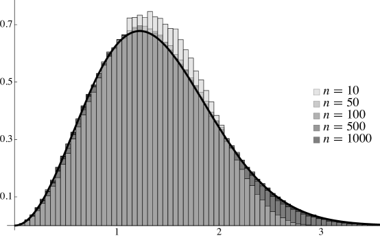
Figure 1: For various $n$, we generated 250,000 random elements of $\operatorname{Arm}(n,3,1)$ and computed $\sqrt{n}\,\|\vec{\mu}\|$, where $\vec{\mu}$ is the geometric median of the edge cloud. By Proposition 9, $\sqrt{n}\,\|\vec{\mu}\|$ converges to a Nakagami$\left(\frac{3}{2},\frac{9}{4}\right)$ distribution, the pdf of which is the solid curve. Though we don’t show it, the behavior in other dimensions is quite similar: by $n=50$ the density of the limiting Nakagami$\left(\frac{d}{2},\left(\frac{d}{d-1}\right)^{2}\right)$ distribution matches the histogram rather well.

Proof.

We start by defining $\operatorname{Ed}(\vec{y})$ to be the expected distance from $\vec{y}\in\mathbb{R}^{d}$ to the unit sphere; formally,

$$\operatorname{Ed}(\vec{y}):=\frac{1}{\operatorname{Vol}S^{d-1}}\int_{\hat{x}\in S^{d-1}}\|\hat{x}-\vec{y}\|\thinspace\operatorname{dVol}_{S^{d-1}}.$$

Observe that, by symmetry, the minimizer of $\operatorname{Ed}(\vec{y})$ is the origin. Now the geometric median of a finite collection of points $\hat{x}_{i}$ uniformly sampled from the sphere is the minimizer of the average distance $\operatorname{Ad}$ to the $\hat{x}_{i}$ (Definition 3). For a large number of points, we expect $\operatorname{Ad}$ to be close to $\operatorname{Ed}$ as a function, and hence that the minimizers of the functions should be nearby as well.

In fact, Niemiro studied exactly this situation, showing ([Niemiro:1992ez, p. 1517], cf. Haberman [Haberman:1989iq]) that

$$\sqrt{n}\,\vec{\mu}\overset{d}{\rightarrow}\mathcal{N}(\vec{0},\mathcal{H}^{-1}V\mathcal{H}^{-1})$$

where $V$ is the covariance matrix of a random point $\hat{x}$ on $S^{d-1}$ and $\mathcal{H}$ is the Hessian of $\operatorname{Ed}$, evaluated at the origin.

The off-diagonal elements of $V$ are zero by symmetry. Using cylindrical coordinates on $S^{d-1}$ with axis $\hat{e}_{i}$, the $i$th diagonal entry in the covariance matrix is computed by the integral

$$\sigma_{i}^{2}=\frac{1}{\sqrt{\pi}}\frac{\Gamma(\frac{d}{2})}{\Gamma(\frac{d-1}{2})}\int_{-1}^{1}x^{2}(1-x^{2})^{\frac{d-3}{2}}\,\,\mathrm{d}x=\frac{1}{d}.$$

We prove in the Appendix (Proposition LABEL:prop:mister_ed) that the expected distance function $\operatorname{Ed}(\vec{y})$ is given as a function of $r=\|\vec{y}\|$ by

$$\operatorname{Ed}(r)=\,_{2}F_{1}\left(-\frac{1}{2},\frac{1-d}{2};\frac{d}{2};r^{2}\right).$$

When $d$ is odd, the standard Taylor series representation of the hypergeometric function truncates, and $\operatorname{Ed}(r)$ is a polynomial in $r$. For example, when $d=3$ we have $\operatorname{Ed}(r)=1+\nicefrac{{r^{2}}}{{3}}$. In turn, a straightforward computation shows that the Hessian of $\operatorname{Ed}$ evaluated at the origin is simply

$$\mathcal{H}=\mathcal{H}\operatorname{Ed}(\vec{0})=\frac{d-1}{d}I_{d},$$

where $I_{d}$ is the $d\times d$ identity matrix. This completes the proof of the first statement. To get the second, we note that the norm of a Gaussian $\mathcal{N}(\vec{0},\sigma^{2}I_{d})$ random variate is Nakagami$\left(\frac{d}{2},d\sigma^{2}\right)$-distributed. ∎

We now see that the geometric median is becoming asymptotically normal, and concentrating around the origin. We can use this to prove an asymptotic result for the distance to closure for equilateral polygons.

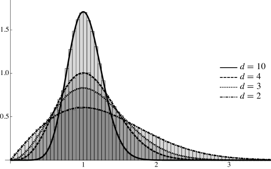
Figure 2: For $d=2,3,4,10$, we generated 250,000 random elements of $\operatorname{Arm}(1000,d,1)$ and computed their chordal distance to $\operatorname{Pol}(1000,d,1)$ using Theorem 8. This plot shows the histograms of chordal distance to closure together with the densities of Nakagami$\left(\frac{d}{2},\frac{d}{d-1}\right)$ distributions.

Proposition 10.

For a random equilateral $n$-gon $\boldsymbol{x}$ with edges $\hat{x}_{i}$ sampled independently and uniformly from $S^{d-1}$, the random variable $d_{\text{chordal}}(\boldsymbol{x},\operatorname{Pol}(n,d,1))$ converges in distribution to a Nakagami$\left(\frac{d}{2},\frac{d}{d-1}\right)$ as $n\rightarrow\infty$.

Proof.

We know from Theorem 8 that $d_{\text{chordal}}(\boldsymbol{x},\operatorname{Pol}(n,d,1))$ is actually the chordal distance from $\boldsymbol{x}$ to $\operatorname{gmc}(\boldsymbol{x})$. To estimate this distance, we will make use of the recentering and renormalizing map $r(\boldsymbol{x},\vec{p},1)$ from Proposition 7.

When $\left\|\mu\right\|$ is small, we can estimate

$$\left\|\operatorname{gmc}(\boldsymbol{x})-\boldsymbol{x}\right\|=\left\|r(\boldsymbol{x};\vec{\mu},1)-r(\boldsymbol{x};\vec{0},1)\right\|\sim\left\|\vec{\mu}\right\|\left\|D_{\hat{\mu}}r(\boldsymbol{x};\vec{0},1)\right\|$$

where $D_{\hat{\mu}}r(\boldsymbol{x};\vec{0},1)$ is the derivative of $r(\boldsymbol{x};\vec{v},1)$ with respect to the vector $\vec{v}$ in the direction of the unit vector $\hat{\mu}=\nicefrac{{\vec{\mu}}}{{\left\|\vec{\mu}\right\|}}$ (while leaving the $\boldsymbol{x}$ variables constant).

Using the definition of $r(\boldsymbol{x};\vec{p},1)$, a direct computation reveals that

$$\left\|D_{\hat{\mu}}r(\boldsymbol{x};\vec{0},1)\right\|=\left(n-\sum_{i}\left<\hat{x}_{i},\hat{\mu}\right>^{2}\right)^{\frac{1}{2}}=\sqrt{n}\left(1-\frac{1}{n}\sum_{i}\left<\hat{x}_{i},\hat{\mu}\right>^{2}\right)^{\frac{1}{2}}.$$

Since $\hat{\mu}$ is a unit vector, the sum is the Rayleigh quotient for the matrix $X=\frac{1}{n}\sum_{i}\hat{x}_{i}\hat{x}_{i}^{T}$, and so obeys the estimates

$$\lambda_{\operatorname{min}}(X)\leq\frac{1}{n}\sum_{i}\left<\hat{x}_{i},\hat{\mu}\right>^{2}\leq\lambda_{\operatorname{max}}(X)$$

Now $\lambda_{\operatorname{min}}(X)$ and $\lambda_{\operatorname{max}}(X)$ are also random variables depending on the $\hat{x}_{i}$, but we can use the matrix Chernoff inequalities [Tropp:2012fb, Remark 5.3] to bound the probability that they are far from $\frac{1}{d}$.

It’s quite standard to prove that $\mathcal{E}(\hat{x}_{i}\hat{x}_{i}^{T})=\frac{1}{d}I_{d}$, so $\mathcal{E}(X)=\frac{1}{d}I_{d}$. The matrix Chernoff inequalities then reduce to

$$\mathcal{P}\left\{\lambda_{\operatorname{min}}(X)<(1-\delta)\frac{1}{d}\right\}\leq d\left(\frac{e^{-\delta}}{(1-\delta)^{1-\delta}}\right)^{\frac{n}{d}}\marginpar{\raggedright\tiny\ref{eq:lmin lower}eq:lminlower}\ignorespaces\@add@raggedright$$ (2)

and

$$\mathcal{P}\left\{\lambda_{\operatorname{max}}(X)>(1+\delta)\frac{1}{d}\right\}\leq d\left(\frac{e^{\delta}}{(1+\delta)^{1+\delta}}\right)^{\frac{n}{d}}\marginpar{\raggedright\tiny\ref{eq:lmax upper}eq:lmaxupper}\ignorespaces\@add@raggedright$$ (3)

For any $\delta>0$, the quantities raised to $\frac{n}{d}$ are $<1$, and so as $n\rightarrow\infty$ the probability that the bounds in (2) and (3) both hold $\rightarrow 1$. In turn, this means that for any fixed $\delta>0$,

$$\mathcal{P}\left\{\left|\frac{1}{d}-\frac{1}{n}\sum_{i}\left<\hat{x}_{i},\hat{\mu}\right>^{2}\right|>\frac{\delta}{d}\right\}\rightarrow 0$$

and so the random variable $\frac{1}{n}\sum_{i}\left<\hat{x}_{i},\hat{\mu}\right>^{2}$ converges in probability to $\frac{1}{d}$. By the continuous mapping theorem, this means that $\left(1-\frac{1}{n}\sum_{i}\left<\hat{x}_{i},\hat{\mu}\right>^{2}\right)^{1/2}\overset{p}{\rightarrow}\sqrt{\frac{d-1}{d}}$.

We can now rewrite the random variable $\left\|\vec{\mu}\right\|\left\|D_{\hat{\mu}}r(\boldsymbol{x};\vec{0},1)\right\|$ as the product of $\left\|\sqrt{n}\,\vec{\mu}\right\|$, which by Proposition 9 converges in distribution to a Nakagami$\left(\frac{d}{2},\left(\frac{d}{d-1}\right)^{2}\right)$ random variable, and $\left(1-\frac{1}{n}\sum_{i}\left<\hat{x}_{i},\hat{\mu}\right>^{2}\right)^{1/2}$, which we have just proved converges in probability to the constant random variable $\sqrt{\frac{d-1}{d}}$.

Using Slutsky’s theorem and a little algebra, this implies that the product converges in distribution to a Nakagami $\left(\frac{d}{2},\frac{d}{d-1}\right)$ random variable, as claimed. ∎

We have now learned something interesting: the distribution of chordal distances to closure should be converging to a distribution which doesn’t depend on the number of edges! This is surprising because the diameter of $\operatorname{Arm}(n,d,1)$ is clearly $\Theta(\sqrt{n})\rightarrow\infty$. This means that some arms might indeed be very far from closure – but they are very rare. We will look for this feature in the more specific probability inequalities to come.

We can also see how fast the tail of the distribution of $d_{\text{chordal}}$ can be expected to decay. The survival function of the Nakagami distribution is an incomplete Gamma function. Using [NIST:DLMF, 8.10.1], we can show that there is a constant $C(d)>0$ so that if $x$ is Nakagami$\left(\frac{d}{2},\frac{d}{d-1}\right)$, then

$$\mathcal{P}\left\{x<t\right\}\geq 1-C(d)\,t^{d-2}e^{-\frac{d-1}{2}t^{2}}.\marginpar{\raggedright\tiny\ref{eq:precise tail bound}eq:precisetailbound}\ignorespaces\@add@raggedright$$ (4)

IV Concentration inequalities for $\left\|\vec{\mu}\right\|$ and $d_{\text{chordal}}$

We now know what to expect in the large-$n$ limit, at least for equilateral polygons: (4) tells us that we should aim for a tail bound for $d_{\text{chordal}}$ which does not depend on $n$ and is proportional to $e^{-\alpha t^{2}}$ for some $\alpha<\frac{d-1}{2}$. We will get exactly such a bound in Corollary LABEL:cor:chordal_concentration at the end of the section. Our bounds will apply for finite $n$, and also apply to the non-equilateral case, where it is not even clear what the large-$n$ limit should mean.

IV.1 A bound connecting $\left\|\vec{\mu}\right\|$ and $d_{\text{chordal}}$.

To start with, we prove a hard bound on the relationship between the geometric median and our two measures of distance in polygon space. First, we note that our procedure of recentering and renormalizing changes each $\hat{x}_{i}$ by a controlled amount.

Lemma 11.

If $\hat{x}_{i}\in S^{d-1}$ and $\vec{p}\in\mathbb{R}^{d}$ is any vector with $\|\vec{p}\|<1$, then $\left\|\hat{x}_{i}-\frac{\hat{x}_{i}-\vec{p}}{\|\hat{x_{i}}-\vec{p}\|}\right\|\leq\sqrt{2}\|\vec{p}\|$ and $\angle(\hat{x}_{i},\frac{\hat{x}_{i}-\vec{p}}{\|\hat{x}_{i}-\vec{p}\|})\leq\arcsin\|\vec{p}\|<\frac{\pi}{2}\|\vec{p}\|$.

Proof.

This is a calculus exercise; it is straightforward to establish the (sharp) bound

$$\left\|\hat{x}_{i}-\frac{\hat{x}_{i}-\vec{p}}{\|\hat{x_{i}}-\vec{p}\|}\right\|\leq\sqrt{2-2\sqrt{1-\|\vec{p}\|^{2}}}.$$

Further, it is easy to check that the right-hand side is a convex function of $\|\vec{p}\|$ which is equal to $0$ when $\|\vec{p}\|=0$, and $\sqrt{2}$ when $\|\vec{p}\|=1$, so it is bounded above by the line $\sqrt{2}\,\|\vec{p}\|$. The angle bound is also straightforward. ∎

We now can give a bound on the distance between a given $\boldsymbol{x}\in\operatorname{Arm}(n,d,w)$ and $\operatorname{Pol}(n,d,w)$ in terms of the norm of the geometric median $\vec{\mu}$ of the edge cloud $(\hat{x}_{i},w_{i})$.

Proposition 12.

If the edge cloud $(\hat{x}_{i},w_{i})$ has geometric median $\vec{\mu}$ with $\|\vec{\mu}\|<1$,

$$d_{\text{chordal}}(\boldsymbol{x},\operatorname{Pol}(n,d,w))<\sqrt{2\sum\omega_{i}^{2}}\,\|\vec{\mu}\|\quad\text{and}\quad d_{\text{max-angular}}(\boldsymbol{x},\operatorname{Pol}(n,d,w))<\arcsin\|\vec{\mu}\|.$$

Proof.

Since $\|\vec{\mu}\|<1$, our polygon is median-closeable and $\operatorname{gmc}(\boldsymbol{x})$ is a closed polygon with edge cloud $\left(w_{i},\frac{\hat{x}_{i}-\vec{\mu}}{\|\hat{x}_{i}-\vec{\mu}\|}\right)$. Lemma 11 immediately yields the bound on $d_{\text{max-angular}}$; to get the chordal distance bound, we write

$$\sqrt{\sum\left\|w_{i}\hat{x}_{i}-w_{i}\frac{\hat{x}_{i}-\vec{\mu}}{\|\hat{x}_{i}-\vec{\mu}\|}\right\|^{2}}\leq\sqrt{\sum w_{i}^{2}\cdot 2\|\vec{\mu}\|^{2}}.$$

∎

IV.2 Strategy for the tail bound

To derive our explicit tail bound on the norm of the geometric median, our strategy is as follows. First, we will prove two probabilistic bounds: an upper bound on $\|\nabla\!\operatorname{Ad}_{\boldsymbol{x}}(\vec{0})\|$ and a positive lower bound on $\lambda_{\operatorname{min}}(\mathcal{H}\operatorname{Ad}_{\boldsymbol{x}}(\vec{0}))$. These will come from scalar and matrix versions of Bernstein’s inequality.

If we restrict $\operatorname{Ad}_{\boldsymbol{x}}$ to a scalar function $\operatorname{Ad}_{\boldsymbol{x}}(z)$ on a ray from the origin, these bounds yield an upper bound on $|\operatorname{Ad}_{\boldsymbol{x}}^{\prime}(0)|$ and a lower bound on $\operatorname{Ad}_{\boldsymbol{x}}^{\prime\prime}(0)$. We will get a uniform lower bound on $\operatorname{Ad}_{\boldsymbol{x}}^{\prime\prime}(z)$ for $z\in[0,\nicefrac{{1}}{{50}}]$ by showing that, $\operatorname{Ad}_{\boldsymbol{x}}^{\prime\prime}(z)\geq\operatorname{Ad}_{\boldsymbol{x}}^{\prime\prime}(0)-7z$ on this interval. We prove this using the special structure of $\mathcal{H}\operatorname{Ad}_{\boldsymbol{x}}$.

By Taylor’s theorem, there is some $z_{*}$ in $[0,z]$ so that

$$\operatorname{Ad}_{\boldsymbol{x}}^{\prime}(z)=\operatorname{Ad}_{\boldsymbol{x}}^{\prime}(0)+z\operatorname{Ad}_{\boldsymbol{x}}^{\prime\prime}(z_{*})\geq-|\operatorname{Ad}_{\boldsymbol{x}}^{\prime}(0)|+\lambda z.$$

This means that for $z>|\operatorname{Ad}_{\boldsymbol{x}}^{\prime}(0)|/\lambda$, this directional derivative must be positive: in particular, since the geometric median $\vec{\mu}$ is by definition a point where $\nabla\!\operatorname{Ad}(\vec{\mu})=\vec{0}$, $\vec{\mu}$ can lie no farther than $|\operatorname{Ad}_{\boldsymbol{x}}^{\prime}(0)|/\lambda$ from the origin.

IV.3 A probabilistic bound on $\|\nabla\!\operatorname{Ad}_{\boldsymbol{x}}(\vec{0})\|=\left\|\sum\omega_{i}\hat{x}_{i}\right\|$

We want to bound the norm of the gradient $\nabla\!\operatorname{Ad}_{\boldsymbol{x}}(\vec{0})$, which we recall from Lemma 5 is equal to $\sum\omega_{i}\hat{x}_{i}$. We will start with a lemma which helps us understand the effect of variable weights $\omega_{i}$.

Lemma 13.

For any collection of $n$ non-negative real numbers $w_{i}$, if we define $\omega_{i}=\nicefrac{{w_{i}}}{{\sum w_{i}}}$,

$$n\geq 1+n^{2}\operatorname{Var}(\omega_{i})=n\sum\omega_{i}^{2}\geq 1,$$

where $\operatorname{Var}(\omega_{i})$ is the variance of $\{\omega_{1},\dots,\omega_{n}\}$. We have equality on the left precisely when all but one of the $w_{i}$ equal zero and equality on the right precisely when all the $w_{i}$ are equal.

Proof of Lemma.

Starting with the definition of variance, and remembering that $\sum\omega_{i}=1$,

$$\operatorname{Var}(\omega_{i})=\frac{1}{n}\sum\omega_{i}^{2}-\left(\frac{1}{n}\sum\omega_{i}\right)^{2}=\frac{1}{n}\sum\omega_{i}^{2}-\frac{1}{n^{2}}$$

Solving for $\sum\omega_{i}^{2}$,

$$\sum\omega_{i}^{2}=\frac{1+n^{2}\operatorname{Var}(\omega_{i})}{n}$$

which proves the central equality. Since $\operatorname{Var}(\omega_{i})\geq 0$ with equality precisely when all the $\omega_{i}$ are equal, the inequality on the right follows easily.

To prove the inequality on the left, we invoke the Bhatia-Davis inequality [Bhatia:2000ge], which says that since the $0\leq\omega_{i}\leq 1$ and the mean of the $\omega_{i}$ is $\nicefrac{{1}}{{n}}$, we have $\operatorname{Var}(\omega_{i})\leq(1-\frac{1}{n})(\frac{1}{n}-0)$ with equality precisely when one $\omega_{i}=1$ and the remainder are zero. ∎

Now we can give our first result:

Proposition 14.

If we have $n$ points $\hat{x}_{i}$ sampled independently and uniformly from $S^{d-1}$, and $n$ weights $\omega_{i}\geq 0$ with $\sum_{i}\omega_{i}=1$ and $\Omega=\max_{i}\omega_{i}$, then for any $t>0$

$$\mathcal{P}\left(\left\|\sum\omega_{i}\hat{x}_{i}\right\|>t\right)\leq d\exp\left(-\frac{3nt^{2}}{2nt\Omega\sqrt{d}+6(1+n^{2}\operatorname{Var}\omega_{i})}\right).$$

If the $\omega_{i}$ are all equal (the polygon is equilateral), this simplifies to

$$\mathcal{P}\left(\left\|\frac{1}{n}\sum\hat{x}_{i}\right\|>t\right)\leq d\exp\left(-\frac{3nt^{2}}{6+2t\sqrt{d}}\right).$$

Proof.

We will use Bernstein’s inequality [Dubhashi:2009ho, Theorem 1.2]: Suppose $X_{1},\dots,X_{n}$ are independent random variables with $X_{i}-\mathcal{E}(X_{i})\leq b$ for each $i$, the variance of each $X_{i}$ is given by $\sigma_{i}^{2}$, and $X=\sum X_{i}$ (with variance $\sigma^{2}=\sum\sigma_{i}^{2}$). Then for any $t>0$,

$$\mathcal{P}\left(X>\mathcal{E}(X)+t\right)\leq\exp\left(-\frac{t^{2}}{2\sigma^{2}\left(1+\frac{bt}{3\sigma^{2}}\right)}\right).$$

For any unit vector $\vec{v}$, we can set $X_{i}=\left<\omega_{i}\hat{x}_{i},\vec{v}\right>$. These random variables clearly have expectation 0 and $X_{i}-\mathcal{E}(X_{i})\leq\omega_{i}\leq\Omega$. Using cylindrical coordinates on $S^{d-1}$ with axis $\vec{v}$, the variance is computed by the integral

$$\sigma_{i}^{2}=\frac{1}{\sqrt{\pi}}\frac{\Gamma(\frac{d}{2})}{\Gamma(\frac{d-1}{2})}\int_{-1}^{1}(\omega_{i}x)^{2}(1-x^{2})^{\frac{d-3}{2}}\,\,\mathrm{d}x=\frac{\omega_{i}^{2}}{d}.$$

Using Lemma 13, this implies

$$\sigma^{2}=\frac{1}{d}\sum\omega_{i}^{2}=\frac{1+n^{2}\operatorname{Var}\omega_{i}}{dn}.$$

This proves that for any $\vec{v}$,

$$\mathcal{P}\left(\left<\sum\omega_{i}\hat{x}_{i},\vec{v}\right>>t\right)\leq\exp\left(-ndt^{2}\frac{3}{6+2\,dnt\,\Omega+6n^{2}\operatorname{Var}\omega_{i}}\right).$$

Applying this inequality $d$ times for $\vec{v}=\hat{e}_{1},\dots,\hat{e}_{d}$, and using the union bound, we can bound the $L^{\infty}$ norm of $\sum\omega_{i}\hat{x}_{i}$:

$$\mathcal{P}\left(\left\|\sum\omega_{i}\hat{x}_{i}\right\|_{\infty}=\max_{j}\left(\sum\omega_{i}\hat{x}_{i}\right)_{j}>t\right)\leq d\exp\left(-ndt^{2}\frac{3}{6+2\,dnt\,\Omega+6n^{2}\operatorname{Var}\omega_{i}}\right).$$

But we know that for any $\vec{u}\in\mathbb{R}^{d}$ we have $\frac{1}{\sqrt{d}}\left\|\vec{u}\right\|\leq\left\|\vec{u}\right\|_{\infty}$, so

$$\mathcal{P}\left(\frac{1}{\sqrt{d}}\left\|\sum\omega_{i}\hat{x}_{i}\right\|>t\right)\leq\mathcal{P}\left(\left\|\sum\omega_{i}\hat{x}_{i}\right\|_{\infty}>t\right)\leq d\exp\left(-ndt^{2}\frac{3}{6+2\,dnt\,\Omega+6n^{2}\operatorname{Var}\omega_{i}}\right).$$

Replacing $t$ by $\frac{t}{\sqrt{d}}$ yields the statement of the Proposition. ∎

The terms $\Omega$ and $\operatorname{Var}\omega_{i}$ in the statement of Proposition 14 at first seem mysterious. However, if you read them in light of Lemma 13, they become clearer.

At one extreme, if one $\omega_{i}$ is close to 1 and the remaining $\omega_{j}$ are small, the sum $\left\|\sum_{i}\omega_{i}\hat{x}_{i}\right\|\sim 1$ regardless of $n$, and $\left\|\sum_{i}\omega_{i}\hat{x}_{i}\right\|$ cannot concentrate on $0$ as $n\rightarrow\infty$. To see this in the statement of the Proposition, observe that in this case $\Omega$ and $\operatorname{Var}\omega_{i}$ approach their maximum values of $\Omega\sim 1$ and $1+n^{2}\operatorname{Var}\omega_{i}\sim n$, the $n$’s in numerator and denominator cancel, and the exponent no longer depends on $n$ at all.

At the other extreme, if the $\omega_{i}$ are all equal, $\Omega$ and $\operatorname{Var}\omega_{i}$ are minimized: $\Omega=\nicefrac{{1}}{{n}}$ and ${\operatorname{Var}\omega_{i}=0}$. In this case, the denominator in the exponent does not depend on $n$ and $\left\|\sum\omega_{i}\hat{x}_{i}\right\|$ concentrates on $0$ as fast as possible. We can compare this result to that of Khoi [Khoi:2005ch], who showed in a different sense that the equilateral polygons are the “most flexible” of all the fixed edgelength polygons.

In the middle, if the $\omega_{i}$ are variable, but the number of comparably large $\omega_{i}$ increases, $\Omega$ and $\operatorname{Var}\omega_{i}$ act to slow the rate of concentration, but they do not stop it: $\left\|\sum_{i}\omega_{i}\hat{x}_{i}\right\|$ still concentrates on $0$ as $n\rightarrow\infty$.

IV.4 A probabilistic bound on $\lambda_{\operatorname{min}}(\mathcal{H}\operatorname{Ad}_{\boldsymbol{x}}(\vec{0}))=\lambda_{\operatorname{min}}\left(I-\sum\omega_{i}\hat{x}_{i}\hat{x}_{i}^{T}\right)$

We now want to bound the lowest eigenvalue of the Hessian of $\operatorname{Ad}_{\boldsymbol{x}}$ at the origin. Again using Lemma 5, we see that $\mathcal{H}\operatorname{Ad}_{\boldsymbol{x}}(\vec{0})=I-\sum\omega_{i}\hat{x}_{i}\hat{x}_{i}^{T}$, where the quantities being summed are outer products of the vectors $\hat{x}_{i}$. That is, they are the symmetric, positive semidefinite projection matrices which project to the lines spanned by the $\hat{x}_{i}$. We now show

Proposition 15.

If we have $n$ points $\hat{x}_{i}$ sampled independently and uniformly from $S^{d-1}$, and $n$ weights $0\leq\omega_{i}$ with $\sum_{i}\omega_{i}=1$ and $\Omega=\max_{i}\omega_{i}$, then for any $t>0$

$$\mathcal{P}\left(\lambda_{\operatorname{min}}\left(I-\sum\omega_{i}\hat{x}_{i}\hat{x}_{i}^{T}\right)>\frac{d-1}{d}-t\right)\leq d\exp\left(-\frac{d}{d-1}\cdot\frac{3dnt^{2}}{2nt\Omega d+6(1+n^{2}\operatorname{Var}\omega_{i})}\right).$$

If the $\omega_{i}$ are all equal (the polygon is equilateral), this simplifies to

$$\mathcal{P}\left(\lambda_{\operatorname{min}}\left(I-\frac{1}{n}\sum\hat{x}_{i}\hat{x}_{i}^{T}\right)>\frac{d-1}{d}-t\right)\leq d\exp\left(-\frac{d}{d-1}\cdot\frac{3dnt^{2}}{2td+6}\right).$$

Proof.

The statement is similar to the statement of Proposition 14, so it should not be surprising that this also follows from a Bernstein inequality, this time for matrices [Tropp:2012fb, Theorem 1.4]: suppose $X_{1},\dots,X_{n}$ are independent random symmetric $d\times d$ matrices, $\mathcal{E}(X_{i})=0$, $\lambda_{\operatorname{max}}(X_{i})\leq b$, the “matrix variance” of each $X_{i}$ is given by $\sigma_{i}^{2}=\mathcal{E}(X_{i}^{2})$, and $X=\sum X_{i}$ (with “scalar variance” $\sigma^{2}=\left\|\sum\sigma_{i}^{2}\right\|$). Then for any $t>0$,

$$\mathcal{P}\left(\lambda_{\operatorname{max}}(X)\geq t\right)\leq d\exp\left(-\frac{t^{2}}{2\sigma^{2}\left(1+\frac{bt}{3\sigma^{2}}\right)}\right)\marginpar{\raggedright\tiny\ref{eq:matrix bernstein}eq:matrixbernstein}\ignorespaces\@add@raggedright$$ (5)

We will set $X_{i}=\omega_{i}\left(\hat{x}_{i}\hat{x}_{i}^{T}-\frac{1}{d}I_{d}\right)$. These are clearly symmetric $d\times d$ matrices.

We now prove $\mathcal{E}(X_{i})=0$. Since the $\hat{x}_{i}$ are uniformly sampled on $S^{d-1}$, their distribution is $O(d)$-invariant. This means we can first average $\hat{x}_{i}$ over any subgroup of $O(d)$ without changing $\mathcal{E}\left(\hat{x}_{i}\hat{x}_{i}^{T}\right)$. We’ll choose the orthotope group of all $2^{d}$ possible diagonal matrices $D$ with $D_{ii}=\pm 1$. For any vector $\vec{v}\in\mathbb{R}^{d}$:

$$\frac{1}{2^{d}}\left(\sum_{D}(D\vec{v})(D\vec{v})^{T}\right)_{ij}=\frac{1}{2^{d}}\sum_{D}D_{ii}D_{jj}v_{i}v_{j}$$

Now for each of the 4 possible combinations of signs $D_{ii}=\pm 1$ and $D_{jj}=\pm 1$, there are the same number $2^{d-2}$ of elements of the orthotope group with these signs. If $i\neq j$, two products are $+1$ and two are $-1$ and the terms cancel. If $i=j$ all the products are the same. Thus the average matrix $\frac{1}{2^{d}}\sum_{D}(D\vec{v})(D\vec{v})^{T}$ is a diagonal matrix with entries $v_{i}^{2}$.

Since the expectation of the square of a coordinate of a randomly distributed unit vector on $S^{d-1}$ was computed in the proof of Proposition 14 to be $\nicefrac{{1}}{{d}}$, we have $\mathcal{E}\left(\hat{x}_{i}\hat{x}_{i}^{T}\right)=\frac{1}{d}I_{d}$, proving that $\mathcal{E}(X_{i})=0$.

We now prove that $\lambda_{\operatorname{max}}(X_{i})\leq\Omega\frac{d-1}{d}$. For any matrix $A$, the eigenvalues of $A+kI_{d}$ are simply $k$ added to the eigenvalues of $A$ (cf. [Horn:2013tf, Theorem 2.4.8.1]). So

$$\lambda_{\operatorname{max}}(X_{i})=\omega_{i}\left(\lambda_{\operatorname{max}}(\hat{x}_{i}\hat{x}_{i}^{T})-\frac{1}{d}\right)=\omega_{i}\frac{d-1}{d}\leq\Omega\frac{d-1}{d}$$

since the largest eigenvalue of a projection matrix like $\hat{x}_{i}\hat{x}_{i}^{T}$ is 1.

Next, we want to show that $\sigma_{i}^{2}=\mathcal{E}(X_{i}^{2})=\omega_{i}^{2}\frac{d-1}{d^{2}}I_{d}$. A direct computation reveals

$$X_{i}^{2}=\omega_{i}^{2}\left(\left(1-\frac{2}{d}\right)\hat{x}_{i}\hat{x}_{i}^{T}+\frac{1}{d^{2}}I_{d}\right)$$

and the result follows from our previous computation that $\mathcal{E}\left(\hat{x}_{i}\hat{x}_{i}^{T}\right)=\frac{1}{d}I_{d}$. Summing the $\sigma_{i}^{2}$ and taking the operator norm, we get

$$\sigma^{2}=\frac{d-1}{d^{2}}\sum\omega_{i}^{2}.$$

Plugging $b$ and $\sigma$ into (5) yields a bound on the probability that $\lambda_{\operatorname{max}}(X)>t$ or, since ${\lambda_{\operatorname{max}}(X)=\lambda_{\operatorname{max}}(\sum\omega_{i}\hat{x}_{i}\hat{x}_{i}^{T})-\frac{1}{d}}$, that $\lambda_{\operatorname{max}}(\sum\omega_{i}\hat{x}_{i}\hat{x}_{i}^{T})>\frac{1}{d}+t$. This completes the proof. ∎

We note that this concentration inequality is better than Proposition 14: there is an extra factor of $d$ in the numerator which means that the concentration gets faster as $d$ increases. The effect of variable edgelengths is to slow (or stop) the concentration, just as in Proposition 14; the same comments on the role of $\Omega$ and $\operatorname{Var}\omega_{i}$ apply here.

IV.5 A bound on the change in the radial second derivative

For any point $\vec{s}\in\mathbb{R}^{d}$, the second derivative of $\operatorname{Ad}_{\boldsymbol{x}}$ along the ray through $\vec{s}$ is given by evaluating the Hessian as a quadratic form on the vector $\vec{s}$ itself. Our last proposition gave us a lower bound on the result at the origin; we now show that this can’t change too fast as we move away from the origin.

Proposition 16.

For $\left\|\vec{s}\right\|<1$ we have

$$\frac{\left<\mathcal{H}\operatorname{Ad}_{\boldsymbol{x}}(\vec{s})\vec{s},\vec{s}\right>}{\left<\vec{s},\vec{s}\right>}-\frac{\left<\mathcal{H}\operatorname{Ad}_{\boldsymbol{x}}(0)\vec{s},\vec{s}\right>}{\left<\vec{s},\vec{s}\right>}\geq-\left\|\vec{s}\right\|\frac{6+\left\|\vec{s}\right\|+\left\|\vec{s}\right\|^{2}}{(1-\left\|\vec{s}\right\|)^{3}}.$$

Since the fraction at right is increasing in $\left\|\vec{s}\right\|$, we can easily simplify the statement given a better upper bound on $\left\|\vec{s}\right\|$. In particular, for $\left\|\vec{s}\right\|<\nicefrac{{1}}{{50}}$, the right-hand side $\geq-7\left\|\vec{s}\right\|$.

Proof.

Using Lemma 5, we see that

$$\left<\mathcal{H}\operatorname{Ad}_{\boldsymbol{x}}(\vec{s})\vec{s},\vec{s}\right>-\left<\mathcal{H}\operatorname{Ad}_{\boldsymbol{x}}(0)\vec{s},\vec{s}\right>=\\ \left(\!\left(\sum\frac{\omega_{i}}{\left\|\hat{x}_{i}-\vec{s}\right\|}\right)-1\right)\left<\vec{s},\vec{s}\right>-\sum\omega_{i}\left(\frac{\left<\hat{x}_{i}-\vec{s},\vec{s}\right>^{2}}{\left\|\hat{x}_{i}-\vec{s}\right\|^{3}}-\left<\hat{x}_{i},\vec{s}\right>^{2}\right).$$

Using the estimates $1-\left\|\vec{s}\right\|\leq\left\|\hat{x}_{i}-\vec{s}\right\|\leq 1+\left\|\vec{s}\right\|$ and recalling that $\sum\omega_{i}=1$, we can underestimate the right hand side by

$$-\frac{\left\|\vec{s}\right\|^{3}}{1+\left\|\vec{s}\right\|}-\sum\omega_{i}\left(\frac{\left<\hat{x}_{i}-\vec{s},\vec{s}\right>^{2}}{(1-\left\|\vec{s}\right\|)^{3}}-\left<\hat{x}_{i},\vec{s}\right>^{2}\right)\geq-\frac{\left\|\vec{s}\right\|^{3}}{1+\left\|\vec{s}\right\|}-\frac{5\left\|\vec{s}\right\|^{3}+\left\|\vec{s}\right\|^{4}+\left\|\vec{s}\right\|^{5}}{(1-\left\|\vec{s}\right\|)^{3}}$$

where the second part follows from finding a common denominator, expanding, and cancelling, using Cauchy–Schwartz carefully to underestimate the inner product terms as needed. Observing that $1+\left\|\vec{s}\right\|>1>(1-\left\|\vec{s}\right\|)^{3}$ allows us to underestimate $-\nicefrac{{\left\|\vec{s}\right\|^{3}}}{{1+\left\|\vec{s}\right\|}}\geq-\nicefrac{{\left\|\vec{s}\right\|^{3}}}{{(1-\left\|\vec{s}\right\|)^{3}}}$, completing the proof. ∎

IV.6 Bounding the norm of the geometric median

We are now in a position to bound the norm of the geometric median! This will proceed in two stages: first, we’ll use the Poincaré–Hopf index theorem to show that $\left\|\vec{\mu}\right\|<\nicefrac{{1}}{{50}}$ under certain hypotheses. Then we can immediately bootstrap to get a sharper bound.

Proposition 17.

If $\left\|\sum\omega_{i}\hat{x}_{i}\right\|=\|\nabla\!\operatorname{Ad}_{\boldsymbol{x}}(\vec{0})\|<\nicefrac{{5}}{{1000}}$, $\lambda_{\operatorname{min}}(\mathcal{H}\operatorname{Ad}_{\boldsymbol{x}}(\vec{0}))>\frac{d-1}{d}-\frac{1}{100}$, and $d\geq 2$, then $\left\|\vec{\mu}\right\|\leq\nicefrac{{1}}{{50}}$.

Proof.

Given our hypothesis on $\lambda_{\operatorname{min}}$ of the Hessian, we know that the $\hat{x}_{i}$ are not all colinear. This means that $\vec{\mu}$ is the unique point inside $S^{d-1}$ where the vector field $\nabla\!\operatorname{Ad}_{\boldsymbol{x}}$ vanishes. We will now show that $\nabla\!\operatorname{Ad}_{\boldsymbol{x}}(\vec{y})$ has a zero inside the sphere of radius $\nicefrac{{1}}{{50}}$; by uniqueness, this point must be the geometric median.

Along any ray from the origin, we may restrict $\operatorname{Ad}_{\boldsymbol{x}}$ to a scalar function $\operatorname{Ad}_{\boldsymbol{x}}(z)$. Using Proposition 16, on the interval $[0,\nicefrac{{1}}{{50}}]$ our hypotheses imply

$$\operatorname{Ad}_{\boldsymbol{x}}^{\prime}(0)\geq-\frac{5}{1000}\quad\text{and}\quad\operatorname{Ad}_{\boldsymbol{x}}^{\prime\prime}(z)\geq\frac{1}{2}-\frac{1}{100}-\frac{7}{50}=\frac{7}{20}.$$

By Taylor’s theorem, there is some $z_{*}\in[0,\nicefrac{{1}}{{50}}]$ so that

$$\operatorname{Ad}_{\boldsymbol{x}}^{\prime}(\nicefrac{{1}}{{50}})=\operatorname{Ad}_{\boldsymbol{x}}^{\prime}(0)+\frac{1}{50}\operatorname{Ad}_{\boldsymbol{x}}^{\prime\prime}(z_{*})\geq-\frac{5}{1000}+\frac{1}{50}\cdot\frac{7}{20}=\frac{2}{1000}>0.$$

This means that the directional derivative of $\operatorname{Ad}_{\boldsymbol{x}}$ in the outward direction is positive on the boundary of the sphere of radius $\nicefrac{{1}}{{50}}$, or that $\nabla\!\operatorname{Ad}_{\boldsymbol{x}}(\vec{y})$ points outward on this sphere. In particular, this implies that the vector field has index 1 on the sphere, and so by the Poincaré–Hopf index theorem must vanish at some point inside the sphere. ∎

We can now prove our main theorem.

Theorem 18.

If we have $n$ points $\hat{x}_{i}$ sampled uniformly on $S^{d-1}$ ($d\geq 2$), $n$ weights $\omega_{i}>0$ so that $\sum\omega_{i}=1$, and $\max\omega_{i}=\Omega$, then for any $t<\nicefrac{{5}}{{1000}}$ we have

$$\mathcal{P}\left(\left\|\vec{\mu}\right\|<\frac{t}{\frac{d-1}{d}-\frac{3}{20}}\right)\geq 1-2d\exp\left(-\frac{3nt^{2}}{2nt\Omega\sqrt{d}+6(1+n^{2}\operatorname{Var}\omega_{i})}\right).\marginpar{\raggedright\tiny\ref{eq:main bound}eq:mainbound}\ignorespaces\@add@raggedright$$ (6)

If all the $\omega_{i}$ are equal (the polygon is equilateral)

$$\mathcal{P}\left(\left\|\vec{\mu}\right\|<\frac{t}{\frac{d-1}{d}-\frac{3}{20}}\right)\geq 1-2d\exp\left(-\frac{3nt^{2}}{2\sqrt{d}t+6}\right).$$

For $d=3$, we have the further simplification

$$\mathcal{P}\left(\left\|\vec{\mu}\right\|<t\right)\geq 1-6\exp\left(-\nicefrac{{nt^{2}}}{{9}}\right).$$

Proof.

We first define two random events: $\lambda_{\operatorname{min}}(\mathcal{H}\operatorname{Ad}_{\boldsymbol{x}}(\vec{0}))>\frac{d-1}{d}-\frac{1}{100}$ (event $A$) and $\left\|\nabla\!\operatorname{Ad}_{\boldsymbol{x}}(\vec{0})\right\|<t<\nicefrac{{5}}{{1000}}$ (event $B$), which will happen for some choices of $\hat{x}_{i}$. Suppose both events occur.

As in Proposition 17, we restrict $\operatorname{Ad}_{\boldsymbol{x}}$ to a scalar function $\operatorname{Ad}_{\boldsymbol{x}}(z)$ on a ray; this time, the ray is assumed to pass through $\vec{\mu}$. By Taylor’s theorem, if we evaluate at $z=\left\|\vec{\mu}\right\|$, there is some $0\leq z_{*}\leq\left\|\vec{\mu}\right\|$ so that

$$0=\mathrm{Ad}{}_{𝒙}{}^{\prime }(\parallel \overrightarrow{\mu }\parallel )=\mathrm{Ad}{}_{𝒙}{}^{\prime }(0)+\parallel \overrightarrow{\mu }\parallel \mathrm{Ad}{}_{𝒙}{}^{\prime \prime }(z{}_{\ast }).$$ (7)