Optimal modularity in complex contagion

Abstract

In this chapter, we apply the theoretical framework introduced in the previous chapter to study how the modular structure of the social network affects the spreading of complex contagion. In particular, we focus on the notion of optimal modularity, that predicts the occurrence of global cascades when the network exhibits just the right amount of modularity. Here we generalize the findings by assuming the presence of multiple communities and an uniform distribution of seeds across the network. Finally, we offer some insights into the temporal evolution of cascades in the regime of the optimal modularity.
Keywords mean-field approximation, social contagions, community structure, linear threshold model, Watts threshold model, optimal modularity

1 Introduction

The previous chapter reviewed the message-passing (MP) framework that can accurately describe the dynamics of spreading processes, and in particular that exhibited by the Watts threshold model Granovetter1978threshold ; Watts2002simple ; gleeson2008cascades . In this chapter, we leverage the framework to study how complex contagions are affected by the modular structure of the underlying social network. In particular, we focus on the notion of optimal modularity, that predicts the occurrence of global cascades when the network exhibits just the right amount of modularity nematzadeh2014optimal .

Modular organization, or community structure, is one of the most ubiquitous properties of real-world networks Girvan2002community ; newman2006modularity and therefore it is crucial to understand how information diffusion is affected by a modular structure. Addressing this problem is particularly urgent when one considers spreading phenomena characterized by complex contagion. Unlike the case of simple contagion, where modules simply slow down the spreading, complex contagion may be either enhanced or hampered by modular structure Centola2010spread ; Weng2013viral . In contrast to simple, complex contagion requires multiple exposures and those are favored within densely connected communities. At the same time, complex contagion can be strongly hampered at the boundaries of communities due to the lack of the sufficient connectivity needed to provide the required multiple exposures from the activated community to the yet-to-be-activated one. The counter-intuitive phenomenon of optimal modularity arises from the clash and compromise between these opposite tendencies.

The basic setting for our study is as follows. We assume a network of individuals where an individual can be in either an “active” or “inactive” state. At each time step, an inactive node may become active if the node is surrounded by enough active nodes. The activation condition is captured in a threshold function $C\left(m,k\right)$ that typically depends on the degree $k$ of a node, and the number $m$ of its active neighbors. Here we consider $C\left(m,k\right)=H(\frac{m}{k}-\theta)$, where $H(x)$ is a Heaviside step function and $\theta$ is a threshold value. Throughout this chapter we assume that $\theta$ is constant across the network. Our analysis leverages the framework introduced in the previous chapter. We focus our analysis only on the ensembles of random networks with arbitrary degree distribution newman2001random , and “message-passing” (MP) and “Tree-Like” (TL) are used interchangeably throughout our chapter.

2 Analytical framework

2.1 Mean-field and message-passing approaches for configuration model

As explained in the previous chapter, the steady-state fraction of active nodes $\rho_{\infty}$ can be estimated using Mean-Field (MF) or the Message-Passing (MP) approaches. Assuming an underlying infinite networks with a given degree distribution $p_{k}$ but otherwise random, $\rho_{\infty}$ can be obtained by solving the following self-consistent equations. Using the MF approach,

$$\rho_{\infty}=\rho_{0}+(1-\rho_{0})\sum_{k}p_{k}\sum_{m=0}^{k}{k\choose m}(\rho_{\infty})^{m}(1-\rho_{\infty})^{k-m}C\left(\frac{m}{k}\right),$$ (1)

where $\rho_{0}$ is the initial fraction of seeds. This approach does not aim at describing the evolution from one time step to the other, rather it states that at stationarity, the density of active nodes is the sum of two contributions: the fraction of seed nodes and expected number of nodes that have an above-the-threshold fraction of active neighbors. This last contribution, in turn, is expressed in terms of the degree distribution and of the density of active nodes itself.

The MP (TL) approach assumes that the underlying network is well approximated by a tree structure. To the extent to which such approximation is valid, where each node is affected only by its children. The density of active nodes depends only from the level of the tree where the node is, which is described by the following formula:

$$q_{n}=\rho_{0}+(1-\rho_{0})\sum_{k}\frac{k}{\langle k\rangle}p_{k}\sum_{m=0}^{k-1}{k-1\choose m}(q_{n-1})^{m}(1-q_{n-1})^{k-1-m}C\left(\frac{m}{k}\right),$$ (2)

where $q_{n}$ is the density of active nodes at the $n$-th level of the tree ($q_{0}=\rho_{0}$). Note that excess degree distribution is used in the place of degree distribution because each node uses one of its link to connect to its parent and only children nodes affect the status of the node. The final density can be calculated by focusing the root node:

$$\rho_{\infty}=\rho_{0}+(1-\rho_{0})\sum_{k}p_{k}\sum_{m=0}^{k}{k\choose m}(q_{\infty})^{m}(1-q_{\infty})^{k-m}C\left(\frac{m}{k}\right),$$ (3)

where $q_{\infty}=\lim_{n\rightarrow\infty}q_{n}$. See the previous chapter for more details.

2.2 Generalization to modular networks

The MP framework can be readily generalized to modular networks by introducing density-of-active variables for each community  gleeson2008cascades . Consider a network with $d$ communities, where the connection probabilities between communities are stored in a $d\times d$ mixing matrix $\mathbf{e}$. Here $e_{ij}$ is the probability that a random edge connects community $i$ and $j$. Consider a node in community $i$ and at the $n+1$ level of the spreading tree. The probability to pick one of its active children ($n$-th level) can be written as:

$$\overline{q}_{n}^{(i)}=\frac{\sum_{j}e_{ij}q_{n}^{(j)}}{\sum_{j}e_{ij}}.$$ (4)

Eq. 2 can be extended to describe the relation between the densities in different communitites gleeson2008cascades .

$$q_{n+1}^{(i)}=\rho_{0}^{(i)}+(1-\rho_{0}^{(i)})\sum_{k}\frac{k}{z^{(i)}}\sum_{m=0}^{k-1}{k-1\choose m}(\overline{q}_{n-1}^{(i)})^{m}(1-\overline{q}_{n-1}^{(i)})^{k-1-m}C^{(i)}\left(\frac{m}{k}\right),$$ (5)

where $z^{(i)}=\sum_{k}kp_{k}^{(i)}$ is the mean degree of community $i$. This set of equations can be solved by iteration analogously to Eq. 3. The density of active nodes at stationarity is:

$$\rho_{\infty}=\sum_{i}\frac{N^{(i)}}{N}\rho_{\infty}^{(i)}.$$ (6)

See gleeson2008cascades for more details.

3 Networks with two communities

Having set up the necessary tool, we now turn into investigating on how the strength of the modular structure can affect the spreading of complex contagion. The simplest setting one may consider is a network with two equally sized communities. Given a fixed and predefined number $L$ of links in the network, we first randomly connect $\mu L$ couple of nodes, where each member of the couple sits in a different community. The remaining links are then used to randomly connect couple of nodes in the same community Girvan2002community . If $\mu=0$, no edge is placed between the two communities (the network has two components and is therefore maximally modular); if $\mu=0.5$, the network is an Erdős-Rényi random graph in the infinite size limit. A fraction $\rho_{0}$ of active nodes are set in one of the two communities, which we call “seed community”.

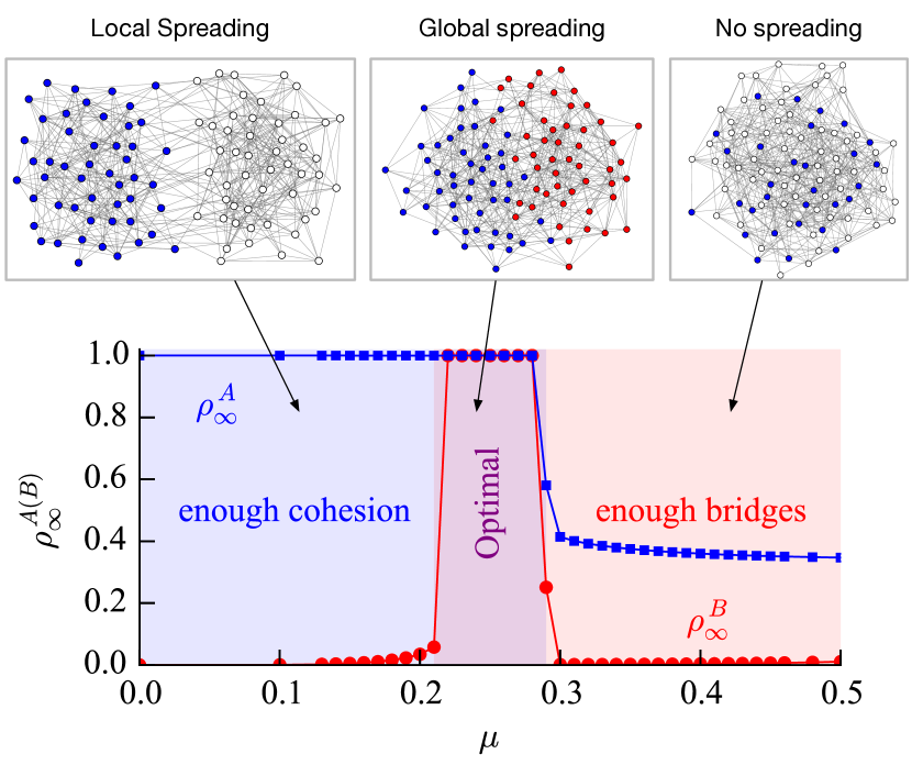
Figure 1: The trade-off between intra- and inter-community spreading. Stronger communities (small $\mu$) facilitate spreading within the originating community while weak communities (large $\mu$) provide bridges that allow spreading between communities. Blue and Red imply activation, while white implies inactivity. There is a range of $\mu$ values that allow both (optimal). The blue squares represents $\rho_{\infty}^{A}$, the final density of active nodes in the community $A$, and the red circles represents $\rho_{\infty}^{B}$. The parameters for the simulation are: $\rho_{0}=0.17$, $\theta=0.4$, $N=131056$, and $\langle k\rangle=20$.

As shown in nematzadeh2014optimal and illustrated in Fig. 1, the density of active nodes at stationarity $\rho_{\infty}$ depends non-trivially on the degree of inter-community connectivity, showing a maximum at intermediate values of $\mu$.

Small values of $\mu$ allow initial spreading in the seed community, but it is essential to have enough mixing (bridges) between communities to have a cascade that significantly interests the global community. At the same time, when too many links across community are present, since these occur at the expense of the intra-community links, there is insufficient connectivity in the seed community to trigger the initial diffusion of the activation. We name optimal modularity the range of $\mu$ values for which the two mechanisms above find their trade-off to maximize the size of the cascade.

4 Optimal modularity in networks with many communities

A network with just two equally sized communities with all the seed users concentrated in one of those is an obvious starting point for this study, but, in general, a non-realistic assumption. We generalize our finding by first considering multiple communities of the same size and with the same degree of intra and inter-connectivity. We then consider a more general process to generate the network and its modular structure. We consider the family of graphs known as LFR (Lancichinetti-Fortunato-Radicchi) benchmark graphs lfr2008bench , which allow us to independently modulate both the size and the degree distribution of the individual communities. We finally remove the constraint of having all seed nodes in a single community.

4.1 Spreading from a seed community

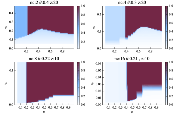
Figure 2: Optimal modularity arises even when there are many communities. The phase diagrams are calculated using the MP framework with different number of communities. ‘nc’ refers the number of communities. $\theta$ and $z$ values are varied to demonstrate the existence of optimal modularity clearly.

Figure 2 and 3 show that the qualitative behavior of $\rho_{\infty}$ as a function of $\mu$ and $\rho_{0}$, when there are two or more communities and the activation is iniated from a single seed community. In general, a larger number of communities requires a smaller adoption threshold to allow the cascade to spread over the all network; increasing the number of communities makes the signal outgoing from the seed community less focused. Such signal, therefore, spreads less easily from community to community. Nevertheless, the same trade-off, and thus optimal modularity, exists between local spreading due to clustering and inter-community spreading due to bridges.

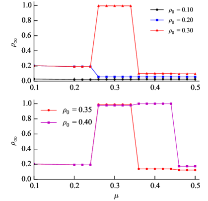
Figure 3: The behavior of threshold model in the presence of community structures generated by LFR benchmark, with $N=25000$, $z=10$, $t_{1}=2.5$ (degree exponent), $t_{2}=1.5$ (community size exponent), $k_{max}=30$ and $\theta=0.3$. LFR benchmark generates more realistic networks with community structures. The degree distribution may have a power-law distribution (with exponent $t_{1}$ and degree cutoff $k_{max}$). The size of the communities may also follow a power-law distribution (with exponent $t_{2}$).

4.2 Spreading from randomly distributed seeds

Next we consider the more general scenario in which the initial signal is distributed across the whole network. The MP approach as described by Eqs. 4 and 5 is sufficiently general to handle the scenario at hand. In particular we will have:

$$\bar{q}_{n}^{(i)}=(1-\mu)q^{(i)}_{n}+\frac{\mu}{(d-1)}\sum_{j\neq i}^{d}q^{(j)}_{n}.$$ (7)

Here $d$ is the number of communities and, as before, $\mu$ represents the total fraction of inter-community bridges in the network. Also, in Eq 5, $\rho_{0}^{(i)}\neq 0$ for all $i$’s rather than just one. The equations can still be solved iterativly.

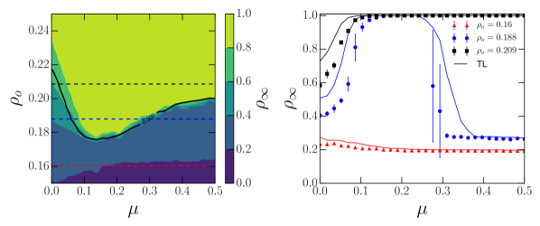
Figure 4: The phase diagram of threshold model with uniformly distributed random seeds. Three example slices are taken from the contour plot (horizontal lines) and displayed in the right figure. $N=25,600$ with $C=160$ communities with $160$ nodes each. The solid black line on the contour shows the MP (TL) results.

Figure 4 shows the results derived via the MP (TL) approach for a network with $25,600$ nodes, $160$ evenly sized communities, and seeds randomly distributed across the network. An optimal region emerges as in the previous multi-community cases.

We would like to note that the optimal region vanishes if each community has exactly same number of seeds; there is no dependence of $\rho_{\infty}$ on $\mu$. The emergence of an optimal region critically depends on the existence of variability across communities. Individual communities show a sharp transition between inactivity and activity as the seed fraction $\rho_{o}$ increases. As all nodes activate essentially simultaneously, the entire system can be regarded as a random network of super-nodes, each representing a single community. The qualitative behavior is therefore the same as that of a random network with no communities. If there is sufficient variability across the communities, in terms of the number of seed nodes they contain then some communities will activate before others and the community structure will have a measurable effect, as shown in Fig 4.

The effect of variability in the nodes’ threshold was actually the focus of the original study of the linear threshold model by Granovetter Granovetter1978threshold . He found that changes in the variance of the threshold distribution leads to qualitatively different spreading behavior even when the mean is kept constant. When variance is low, nodes have approximately the same threshold and, all other factors being the same, they get activated more or less simultaneously. Higher variance brings the existence of a continuum spectrum from low to high threshold nodes. Low threshold are typically activated first and can help the activation of nodes with slightly higher threshold. In turn, these can contribute to activate even higher threshold nodes, and possibly generate a large size cascade. But if threshold variance is too high, the gap between low threshold and high threshold nodes is too large and the activation of the former is not sufficient to fill the gap in threshold.

Given the tendency of nodes in a community to activate simultaneously, it is possible to regard them as coarse-grained super-nodes whose threshold is effectively determined by the number of seeds they contain. This formulation provides similar insights as the Granovetter’s study Granovetter1978threshold . We investigated this idea by distributing seeds across communities according to a Beta distribution. We fix the $\alpha$ and $\beta$ parameters for the Beta distribution in such a way to maintain the expected value constant at $\langle\rho_{o}\rangle=0.19$ while the standard deviation ($\sigma$) is varied.

Our experiments, as shown in Figure 5 produce results qualitatively similar to those for Granovetter’s model Granovetter1978threshold .

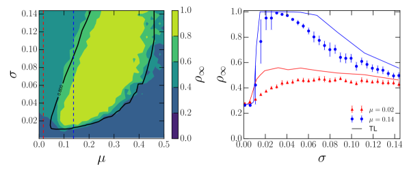
Figure 5: The phase diagram of threshold model with beta distributed random seeds. Two example slices are taken from the contour plot (vertical lines) and displayed in the right figure. The mean seed $\langle\rho_{o}\rangle=0.19$. Numerical simulations were done with $N=25600$ with $C=160$ communities with $160$ nodes each. The solid black line on the contour shows the MP results.

Specifically, Fig. 5 shows that two optimal behaviors emerge, one with respect to $\sigma$ and one with respect to $\mu$. The peak along $\sigma$ arises for exactly the reasons exposed above. A large cascade can be triggered for intermediate values of $\sigma$, when there is a continuum spectrum of effective activation thresholds across communities. Due to a cascading effect, increasing activity within the network makes it more likely to activate communities with fewer and fewer seeds. When $\sigma$ is low communities have roughly the same number of seeds and none have enough seeds to fully activate unless the mean number of seeds is increased. At high $\sigma$, communities with many seeds activate, but they don’t generate enough cumulative activity to activate the low seed communities.

The optimal region with respect to $\mu$ arises for the same trade-off to those studied above. Low $\mu$ implies strong connectivity inside single communities, but insufficient bridges to spread the activation signal externally. For high $\mu$ there are bridges, but not sufficient internal connectivity in order to trigger the initial activation of a sufficiently large number of communities. An optimal balance is achieved at intermediate values of $\mu$.

5 Temporal aspects of optimal modularity

How fast a contagion can spread is often as important as how far it can spread. Imagine, for example, the sudden availability of a prophylactic measure in the wake of a pandemic. The issue would then be not just whether this measure can spread broadly, but also whether it can spread sufficiently fast to effectively oppose the pandemic. Here we limit our study to the basic setting consisting of two communities with varying degree of modularity ($\mu$) and only one seed community. We measure the total diffusion time: the number of time steps needed for the system to reach a steady state. We run a 1,000 simulations (each with an independent network realization) and measure the mean $\rho_{\infty}$ and total diffusion time. We also assume a uniform threshold ($\theta=0.4$).

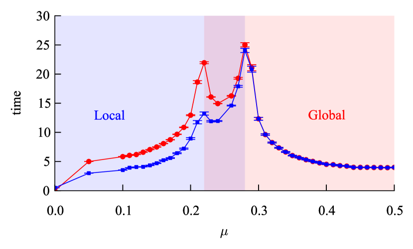
Figure 6: Total diffusion time and optimal modularity. The blue symbols and line represent the total diffusion time in the community $A$ (seed community), and the red symbols and line represent the total diffusion time in the community $B$ (the other community). The optimal modularity range that allows global cascades is represented with a purple shade. The total diffusion time curve peaks at the two transition points, demonstrating that there exists a narrower range of $\mu$ values where the global cascades happen, faster. The parameters for the simulation are: $\rho_{0}=0.17$, $\theta=0.4$, $N=8,192$, and $z=20$.

Figure 6 demonstrates that while $\rho_{\infty}$ remains constant at its maximum value, the total diffusion time greatly varies. Close to either border of the optimal range, contagion significantly slows down, while the global spreading can happen fastest near the middle of the optimal modularity regime. When there are just enough bridges (the left border), the spreading from the seed community to the other community is slower than the case where there are more than just enough bridges to spare (center). Similarly, when there are just enough local cohesion (the right border), the local spreading produces just enough newly activated nodes to achieve global cascade, slowing down the spreading process.

6 Discussion

In this chapter, we have generalized the optimal modularity phenomena and studied its temporal aspect. We showed that many simplifying assumption made in the original study can be relaxed without disrupting the qualitative scenario that predicts a maximum in the fraction of active individuals for intermediate values of inter-community connectivity. In particular we considered the case of a large number of communities, with heterogeneous size, and non uniform degree of initial activation.

Our experiment showed that our model behaves qualitatively same as one in which communities can be considered as super-nodes and are characterized by different threshold. This, in turn, may open the possibility to study very large system if one could devise a strategy to compute the effective parameters of a coarse grained model where communities are represented by single nodes. The interest in developing such ”renormalization” techniques is not only theoretical: threshold models have found several application to real world problems, including the multi-scale modeling of brain networks sporns2004brain and of their activation dynamics in the brain hilge2011hmn .

References

- [1] Mark Granovetter. Threshold models of collective behavior. Am. J. Sociol., 83(6):1420–1443, 1978.
- [2] D.J. Watts. A simple model of global cascades on random networks. Proc. Nat. Acad. Sci., 99(9):5766, 2002.
- [3] James P Gleeson. Cascades on correlated and modular random networks. Physical Review E, 77(4):046117, 2008.
- [4] Azadeh Nematzadeh, Emilio Ferrara, Alessandro Flammini, and Yong-Yeol Ahn. Optimal network modularity for information diffusion. Physical review letters, 113(8):088701, 2014.
- [5] M. Girvan and M.E.J. Newman. Community structure in social and biological networks. Proc. Nat. Acad. Sci., 99(12):7821, 2002.
- [6] Mark EJ Newman. Modularity and community structure in networks. Proceedings of the national academy of sciences, 103(23):8577–8582, 2006.
- [7] Damon Centola. The spread of behavior in an online social network experiment. Science, 329(5996):1194–1197, 2010.
- [8] L. Weng, F. Menczer, and Y.-Y. Ahn. Virality prediction and community structure in social networks. Sci. Rep., 3:2522, 2013.
- [9] Mark EJ Newman, Steven H Strogatz, and Duncan J Watts. Random graphs with arbitrary degree distributions and their applications. Physical review E, 64(2):026118, 2001.
- [10] A. Lancichinetti, S. Fortunato, and F. Radicchi. Benchmark graphs for testing community detection algorithms. Phys. Rev. E, 78:046110, 2008.
- [11] O. Sporns, D. R. Chialvo, M. Kaiser, and C. C. Hilgetag. Organization, development and function of complex brain networks. Trends in Cognitive Sciences, 8(9):418–425, 2004.
- [12] S.-J. Wang, C. C. Hilgetag, and C. Zhou. Sustained activity in hierarchical modular neural networks: self-organized criticality and oscillations. Frontiers in Computational Neuroscience, 5(30):1–14, 2011.