Atom-optics knife-edge:
Measuring narrow momentum distributions

Abstract

By employing the equivalent of a knife-edge measurement for matter-waves, we are able to characterize ultra-low momentum widths. We measure a momentum width corresponding to an effective temperature of 0.9 $\pm$ 0.2 nK, limited only by our cooling performance. To achieve similar resolution using standard methods would require hundreds of milliseconds of expansion or Bragg beams with tens of Hz frequency stability. Furthermore, we show evidence of tunneling in a 1D system when the “knife-edge” barrier is spatially thin. This method is a useful tool for atomic interferometry and for other areas in cold-atom physics where a robust and precise technique for characterizing the momentum distribution is crucial.

I Introduction

Over the last decades, atomic physics has borrowed techniques and concepts from optics: atom lasers Mewes et al. (1997); Bloch et al. (1999); Hagley et al. (1999); Köhl et al. (2001, 2005); Billy et al. (2007); Bouyer et al. (2002), atom interferometry Dickerson et al. (2013); Kovachy et al. (2015a); McDonald et al. (2013); Müntinga et al. (2013); M. R. Andrews, C. G. Townsend, H.-J. Miesner, D. S. Durfee, D. M. Kurn (1997), and matter-wave lensing Ammann and Christensen (1997); Chu et al. (1986); Maréchal et al. (1999); Myrskog et al. (2000); Morinaga et al. (1999), to mention a few of them. Matter-wave lensing, also known as delta-kick cooling (DKC), allows for a decrease in the effective temperature of the atoms by applying a “lens” to collimate the atomic cloud. This technique has been particularly useful for matter-wave interferometry, where the decrease in temperature translates to longer coherence times. It is also of interest to other areas where there is a stringent requirement on the momentum width Carusotto (2001); Jachymski et al. (2018). The temperatures obtained with delta-kick cooling have been pushed lower and lower in recent years, achieving temperatures in the sub-nanokelvin regime Kovachy et al. (2015b), well below standard cooling techniques. This achievement comes hand in hand with the challenge of measuring such low temperatures. Standard time-of-flight (TOF) measurements become inadequate for characterizing the momentum distribution of the atoms, as the expansion time necessary to determine it precisely increases to hundreds of milliseconds or even seconds [Fig. 1b].
In this article, we present an alternative technique to characterize the momentum distribution. This technique had been envisioned before in Billy et al. (2007). Following an atom-optics approach, this method relies on performing a knife-edge scan of the momentum distribution of the atoms with the help of a repulsive potential. A sufficiently thick barrier transmits only atoms with energies greater than the potential height, a momentum-space analog of the optical knife-edge. This method does not depend on the long interrogation times or high phase stability required by methods such as TOF or Bragg spectroscopy Stenger et al. (1999).

II Knife-edge technique

In optics, a common method to determine a beam radius is to scan a sharp edge across the beam path and detect the transmitted power. This technique is called knife-edge measurement. A general expression for the detected signal is

$$P(x^{\prime})=\int_{-\infty}^{\infty}I(x)R(x-x^{\prime})dx,$$ (1)

where $R(x)$ is the transmission function of the razor blade, and $I(x)$ is the beam intensity profile. This equation is a convolution of the transverse profile of the optical beam and the transmission function of the knife-edge, which for an opaque and sharp razor blade resembles a step function. Thus the detected signal is the integrated intensity profile of the optical beam, an error function for a gaussian beam.

In the case of an atomic knife-edge measurement, the spatial distribution of the optical beam is replaced by the velocity distribution of an atomic wave packet and a gaussian barrier plays the role of the razor blade. In contrast with a square barrier, the transmission through a gaussian potential does not exhibit any sharp resonances [Fig. 1c], and lacks a closed-form expression. Nevertheless, for a thick gaussian barrier, the transmission approaches a step function, thus acting effectively as a high-pass velocity filter. Therefore, the transmission for a dilute condensate is approximated by

$$T(v)=\frac{1}{2}\left[1+\operatorname{erf}\left(\frac{v-v_{barrier}}{\sqrt{2}\sigma_{at}}\right)\right],$$ (2)

where $v$ is the relative velocity of the atoms with respect to the barrier, $v_{barrier}$ is the velocity corresponding to the barrier height and $\sigma_{at}$ is the atomic rms velocity width. This expression is exact for an non-interacting ensemble. Additionally, the measured rms velocity width $\sigma_{at}$ does not depend on the potential height [Fig. 1c], making this technique flexible as the potential height does not require day to day calibration.

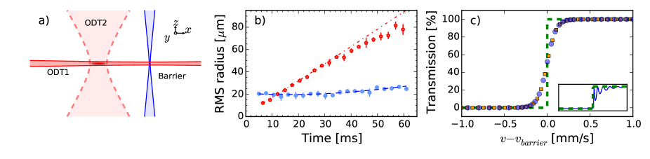
Figure 1: (a) Experimental setup: atoms are initially trapped in a crossed dipole trap formed by the ODT1 and ODT2 beams. During the experiment, the ODT2 beam is turned off, and a magnetic field gradient is used to push the atoms along the waveguide (ODT1) and towards the barrier. (b) Time-of-flight measurements of a cloud without cooling with a temperature of 15 nK (red hexagons), and a cloud after delta-kick cooling with a temperature of 1.3 nK (blue dots). (c) Calculated transmission through a thick (3.1 $\mu$m) gaussian barrier for two different barrier heights: 50 nK (orange squares) and 500 nK (blue dots), and transmission through a 3.1 $\mu$m square potential (inset). The dashed line is a step function for comparison with the transmission through a gaussian barrier (square barrier - inset).

III Experimental system

In our experiment, we prepare a ⁸⁷Rb Bose-Einstein condensate in a 1064 nm crossed dipole trap, with all the atoms in the $|F=2,m_{F}=2\rangle$ state [Fig. 1a]. One of the optical dipole trap beams (ODT1) creates a quasi 1D waveguide for the atoms with trap frequencies $\nu_{r}=217$ Hz and $\nu_{l}=2.7$ Hz, while the other trap beam (ODT2) provides initial confinement of $\nu_{l_{2}}=61$ Hz along the longitudinal waveguide direction. After creating a pure BEC, we perform additional forced evaporation down to $3\times 10^{4}$ atoms to lower the interaction energy. This last evaporation results in a narrower initial momentum distribution while keeping a high signal-to-noise ratio in the absorption images.

A thin sheet of light, propagating along the $z$-direction, intersects the waveguide and produces a repulsive potential [Fig. 1a]. This potential, described in detail in Ref. Potnis et al. (2017), is a 405 nm beam that is focused tightly along the $x$-direction, and scanned in the $y$-direction using an acousto-optic modulator to create a flat average potential over a 75 $\mu$m region. This beam has been characterized outside the experiment, giving a $1/e^{2}$ radius of 1.3 $\mu$m and a Rayleigh range of 8 $\mu$m. By scanning the barrier along the $z$-direction and colliding the atoms with it, we locate the waist of the beam.

IV Momentum width characterization

We prepare a particular velocity width for the atomic wavepacket through delta-kick cooling. In short, DKC is the temporal matter-wave analog of an optical lens: atoms are allowed to expand for a time $T$, then a harmonic potential with frequency $\omega$ “kicks” the atoms for a duration $\tau$, mimicking a lens with “focal time” $f=1/\omega^{2}\tau$. If $\omega$ and $\tau$ are adjusted such that $f=T$, then the cloud is collimated, achieving a minimum velocity spread which is reduced by the ratio of the final cloud to the initial cloud size Ammann and Christensen (1997); Chu et al. (1986); Maréchal et al. (1999); Myrskog et al. (2000); Morinaga et al. (1999). In our experiment, we realize a two kick sequence that provides finer control to scan around the best kick duration. This sequence also yields better performance than a single kick in our setup. The cycle starts when atoms are released from the crossed dipole trap by turning the ODT2 beam off and allowed to expand in the waveguide for 12 ms. This initial expansion time is long enough to convert the interaction energy into kinetic energy ($t_{exp}>1/\omega_{l2}$). The ODT2 beam is then flashed for 1 ms, applying an initial kick to the cloud, but not fully collimating the momentum distribution. The atoms continue to expand for another 15 ms, and finally, a second kick with half the power of the first kick is applied for a variable time. The amount of expansion is limited by the radius of the ODT2 beam (100 $\mu$m): this expansion time is kept short for the atoms to be within the harmonic region of the gaussian potential. Ultimately, we found through comparison with numerical simulations of the Gross-Pitaevskii equation (GPE) that the cooling efficiency in our setup is not limited by the initial cloud expansion; a possible explanation is high spatial frequency perturbations in the delta-kick cooling beam which could lead to forces comparable to that of the lensing kick Kovachy et al. (2015b).

For the velocity width measurements, the repulsive potential is positioned off-focus to obtain a barrier width of 3.1 $\mu$m. The thickness of the potential ensures that tunneling is negligible and the barrier serves as a sharp momentum filter. Atoms will be transmitted if and only if their kinetic energy exceeds the barrier height.

After the preparation of the atomic wavepacket, the barrier height is ramped up to its final value. For the experimental sequence, it is sufficient to vary either the barrier height or the incident velocity of the atoms. Given power limitations on the barrier beam, we chose to scan the incident velocity of the atoms while keeping the barrier height fixed. A variable strength magnetic field gradient is pulsed for 0.5 ms along the longitudinal axis of the waveguide to control the incident velocity of the atoms. For the typical velocities in the experiment, the ensemble takes 6-8 ms to arrive at the barrier and 1-3 ms to transverse the barrier. After the interaction is complete, an absorption image is taken to measure the transmitted and reflected portions. Finally, using Eq. 2, we fit this data to extract the barrier height and the velocity width of the atomic ensemble.

IV.1 Results

We compare our method to the standard TOF measurement. The latter technique consists of the same DKC sequence, followed by expansion times up to 60 ms. The maximum expansion time is based on the requirement that the atoms remain in the waveguide and do not experience any further lensing from its weak longitudinal harmonic confinement. The fit function for the rms radius in the TOF measurement is $\Delta x(t)=\sqrt{{{\Delta x_{0}}^{2}+\Delta v^{2}(t-t_{0})^{2}}}$, where $\Delta x_{0}$ is the minimum atomic rms radius, $\Delta v$ is the atomic rms velocity width and $t_{0}$ is the time at which the atoms focus to their minimum rms radius. TOF and knife-edge measurements for a given kick duration are interleaved and randomized to avoid any possible fluctuations that might affect solely one of the techniques.

We identify three distinct regimes when the kick strength is varied in the cooling sequence: (I) underkicked, (II) close to ideal kick and (III) overkicked. In the underkicked regime [Fig. 2b, yellow region], the TOF measurement is not a robust way to obtain the momentum width as a small amount of noise in the measured cloud radius can severely affect the ability to estimate the fit parameters correctly. This can be understood by recognizing that two of the fit parameters ($\Delta x_{0}$ and $t_{0}$) become highly correlated in this regime and are difficult to estimate independently, and as a result, the TOF technique displays large uncertainties. For the points close to the ideal kick [Fig. 2b, orange region], the two techniques agree though the TOF measurements yield uncertainties about three times larger than the knife-edge technique [Fig. 2b, inset]. The TOF error bars are caused mainly by the constraint of low expansion times, which renders it difficult to estimate these low-velocity widths precisely. The resolution of the knife-edge technique is 0.03 mm/s, corresponding to a temperature resolution of 200 pK. The resolution is limited by the reproducibility in our cooling sequence, not by the knife-edge technique. Finally, in the overkicked region [Fig. 2b, green region], the discrepancy in the measurements comes from the fast rate of expansion after focusing caused by interactions and the extra kick due to the weak harmonic confinement along the waveguide. This additional kick is minimized in the knife-edge technique because of the short interaction time. These observations are backed up qualitatively by GPE simulations [Fig. 2c], though a quantitative comparison would require incorporating the specific imperfections in our lensing beam, which are not included in these simulations.

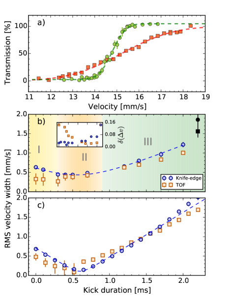
Figure 2: Velocity width measurement. (a) Knife edge measurement: transmission through a thick gaussian barrier for a 0.7 ms kick duration (green circles) and without cooling (red squares). (b) Different amount of cooling is performed by adjusting the kick duration of the second DKC pulse. Blue circles correspond to knife-edge measurements while red squares are TOF measurements, black solid circle (square) shows a measurement without the cooling sequence. The dashed blue line is a quadratic fit, and serves as a guide to the eye. Inset: Uncertainties for the velocity width measurements in mm/s, horizontal axis same as Fig. 2b. (c) 1D Gross-Pitaevskii simulations for the same velocity width measurements. These simulations follow the same sequence and analysis as the experimental data. Color coding is the same as Fig. 2b.

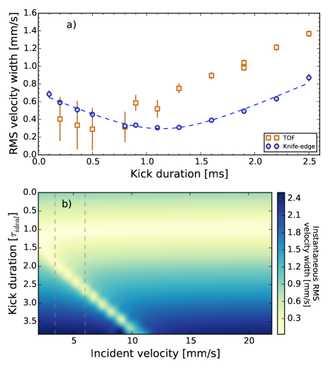
Figure 3: Mean field effect on velocity width measurement. (a) Experimental data. Blue circles correspond to knife-edge measurements taken when atoms focus at the barrier, which is located 120 $\mu$m away, while red squares are TOF measurements. Some error bars are smaller than the symbols. The dashed blue line is a quadratic fit. (b) GPE simulations of the velocity width at the instant the atoms reach the barrier, which is determined by the incident velocity (horizontal axis). This is shown for a range of kick durations (vertical axis). The region in between the dashed lines is where the points for the knife-edge measurement in Fig 3a were taken.

IV.2 Mean-field effect

As shown in the previous section, the knife-edge technique is simple to implement and provides a precise measurement of the atomic momentum width, but the effect of interactions must be considered as it can alter the behaviour of a system significantly Burger et al. (1999); Arnold and Moore (2001); Kashurnikov et al. (2001); Potnis et al. (2017); Chevy and Salomon (2016). In the results from section IV.1, the effects due to interactions are negligible, and it is only when the matter-wave lens focuses the cloud that these effects come into play, due to an increase in the atomic density.

We have taken additional measurements in the overkicked regime, where the atom cloud focuses, to explore this effect. The cooling sequence is similar to the one previously described. The incident velocities were chosen so that the cloud would collide with the barrier close to the time at which it is focused to its minimum width. Fig. 3a shows a series of measurements carried out in the range of incident velocities indicated by the two gray dashed lines in Fig. 3b. The knife-edge measurement yields lower velocity widths than the TOF measurements, and the apparent ideal kick duration is biased towards longer kick durations due to the points in the region where the kinetic energy converts to interaction energy. This is confirmed by GPE simulations [Fig. 3b] which show that the instantaneous velocity width decreases considerably in the regions where the cloud focuses.

IV.3 Comparison with other techniques

The high precision of the knife-edge technique can be seen in Fig. 2. It is only when the velocity width is too large (sequence without DKC or long kick durations) that the uncertainties grow due to the scarcity of points at the wings of the transmission function. The sources of error that could play a role were monitored in each shot. The fluctuations of the magnetic gradient pulse used to push the atoms are lower than 1%, and the power fluctuations on the barrier beam are kept below 1.5 % in each knife-edge scan.

The knife-edge technique shows a clear advantage over the TOF measurement. To precisely determine the velocity width of the atoms using TOF, the expansion time has to be much greater than $\Delta x_{o}/\Delta_{v}$, which in the case of our lowest velocity width corresponds to $\gg$ 60 ms. In most cases, the long expansion time restricts this measurement [Fig. 1b], with a few notable exceptions, for instance in experiments where the expansion is conducted in a microgravity environment van Zoest et al. (2010) or a long vacuum chamber Zhou et al. (2011); Dickerson et al. (2013).

Bragg spectroscopy is another standard tool for obtaining the velocity spread of an atomic cloud. Atoms moving at a velocity $v$ are diffracted by two beams with a relative angle $\theta$ and a frequency difference given by

$$\Delta\omega=\frac{2\hbar k^{2}}{m}+2kv\sin\theta,$$ (3)

where $k$ is the light wavevector, and $m$ is the atomic mass. The last term corresponds to the Doppler shift, which allows for mapping of the velocity distribution. Given the obtained atomic velocity width, the frequency difference to map out the velocity distribution with a 0.03 mm/s resolution, would correspond to 10’s of Hz. The frequency stability required to diffract the atoms of a particular velocity class, plus the power stability to maintain the same Rabi frequency, make this technique demanding for narrow atomic velocity widths.

V Tunneling

Tunneling drives the dynamics in a number of systems in ultracold atoms: from spatial tunneling in the Bose-Hubbard model Greiner et al. (2002) to tunneling in phase space in nonlinear systems Hensinger et al. (2001). However, a textbook situation where, in a one-dimensional system, a wavepacket impinges and tunnels through a potential barrier had not been realized in ultracold atoms before due to the constraints in the velocity width of the impinging wavepacket, and the exponential decrease of tunneling with barrier thickness.

In the previous sections, we discussed the transmission through a thick barrier and how we can use it to characterize the atomic velocity width. For a thin barrier, Eq. 2 is no longer valid, as tunneling becomes relevant and modifies the transmission. The width of the transmission function is given by $\sigma=\sqrt{\sigma_{at}^{2}+\sigma_{b}^{2}}$, where $\sigma_{b}$ depends on the barrier width and accounts for tunneling in the system. Tunneling causes a thin barrier to behave as a “blunt” knife-edge as it blurs out the cut-off of the atomic velocity profile. Transfer matrix and 1D GPE simulations of a wavepacket transmission for different barrier widths are shown in Fig. 4a. The dependence of $\sigma$ on the barrier width is as expected; tunneling becomes a more significant correction for thin barriers, while it vanishes rapidly as the thickness increases, thus recovering the atomic velocity width.

We have found evidence of tunneling in our system through the dependence of the observed velocity width on the barrier thickness. Fig. 4b shows predictions for the measured velocity width as a function of the wavepacket velocity width. The extracted rms velocity width from 1D GPE simulations agrees with the behaviour expected from the quadrature sum of the atomic velocity width $\sigma_{at}$ and the contribution due to tunneling $\sigma_{b}$, where $\sigma_{b}$ for a 1.3 $\mu$m barrier is about two times greater than that of a 3.1 $\mu$m barrier [Fig 4a - blue diamonds]. We measured the momentum width for the cases of a barrier width of 1.3 $\mu$m and 3.1 $\mu$m [Fig. 4b], and found that the two results differ by two standard deviations. Our measurements agree with the difference of the momentum width expected from the simulations [Fig. 4b inset], and are thus consistent with tunneling through a 1.3 $\mu$m barrier.

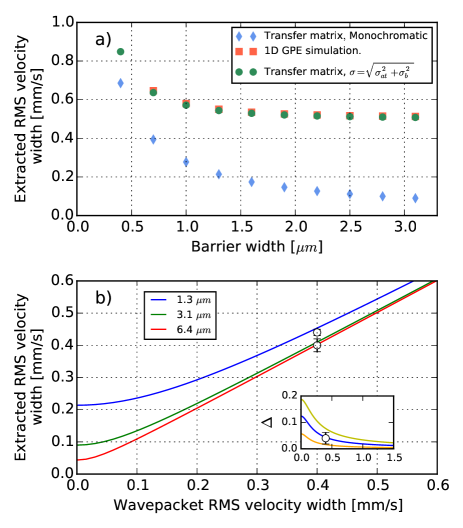
Figure 4: (a) Knife-edge extracted rms velocity width as a function of the barrier width. The simulations were done for a wavepacket with an atomic velocity width $\sigma_{at}=$ 0.5 mm/s, with the exception of the monochromatic transfer matrix calculation. (b) Knife-edge extracted rms velocity against the incident wavepacket velocity width, hollow dots represent experimental measurements. Inset: Velocity width difference $\Delta$ vs. wavepacket rms velocity width for a 1.0 $\mu$m (yellow), 1.3 $\mu$m (blue) and 1.9 $\mu$m (orange) barrier with a 3.1 $\mu$m barrier.

VI Conclusions

We have demonstrated a technique to characterize ultralow velocity widths corresponding to a resolution in temperature of 200 picokelvin. We expect this tool to be beneficial for atom interferometry as it is straightforward to implement, robust in comparison with spectroscopic techniques, and provides a direct measurement of the velocity width with high precision on desirable experimental timescales. Additionally, we observe evidence of tunneling in a quasi 1D system in scattering configuration. This system should permit novel studies of foundational questions in quantum mechanics Steinberg (1995a, b).

References

- Mewes et al. (1997) M.-O. Mewes, M. R. Andrews, D. M. Kurn, D. S. Durfee, C. G. Townsend, and W. Ketterle, Phys. Rev. Lett. 78, 582 (1997).
- Bloch et al. (1999) I. Bloch, T. W. Hänsch, and T. Esslinger, Phys. Rev. Lett. 82, 3008 (1999).
- Hagley et al. (1999) E. W. Hagley, L. Deng, M. Kozuma, J. Wen, K. Helmerson, S. L. Rolston, and W. D. Phillips, Science 283, 1706 (1999).
- Köhl et al. (2001) M. Köhl, T. Hänsch, and T. Esslinger, Phys. Rev. Lett. 87, 160404 (2001).
- Köhl et al. (2005) M. Köhl, T. Busch, K. Mølmer, T. W. Hänsch, and T. Esslinger, Phys. Rev. A 72, 063618 (2005).
- Billy et al. (2007) J. Billy, V. Josse, Z. Zuo, W. Guerin, A. Aspect, and P. Bouyer, Ann. Phys. Fr. 32, 2 (2007).
- Bouyer et al. (2002) P. Bouyer, S. A. Rangwala, J. H. Thywissen, Y. Le Coq, F. Gerbier, S. Richard, G. Delannoy, and A. Aspect, J. Phys. IV 12, 115 (2002).
- Dickerson et al. (2013) S. M. Dickerson, J. M. Hogan, A. Sugarbaker, D. M. S. Johnson, and M. A. Kasevich, Phys. Rev. Lett. 111, 083001 (2013).
- Kovachy et al. (2015a) T. Kovachy, P. Asenbaum, C. Overstreet, C. A. Donnelly, S. M. Dickerson, A. Sugarbaker, J. M. Hogan, and M. A. Kasevich, Nature 528, 530 (2015a).
- McDonald et al. (2013) G. D. McDonald, C. C. N. Kuhn, S. Bennetts, J. E. Debs, K. S. Hardman, M. Johnsson, J. D. Close, and N. P. Robins, Phys. Rev. A 88, 053620 (2013).
- Müntinga et al. (2013) H. Müntinga, H. Ahlers, M. Krutzik, A. Wenzlawski, S. Arnold, D. Becker, K. Bongs, H. Dittus, H. Duncker, N. Gaaloul, C. Gherasim, E. Giese, C. Grzeschik, T. W. Hänsch, O. Hellmig, W. Herr, S. Herrmann, E. Kajari, S. Kleinert, C. Lämmerzahl, W. Lewoczko-Adamczyk, J. Malcolm, N. Meyer, R. Nolte, A. Peters, M. Popp, J. Reichel, A. Roura, J. Rudolph, M. Schiemangk, M. Schneider, S. T. Seidel, K. Sengstock, V. Tamma, T. Valenzuela, A. Vogel, R. Walser, T. Wendrich, P. Windpassinger, W. Zeller, T. van Zoest, W. Ertmer, W. P. Schleich, and E. M. Rasel, Phys. Rev. Lett. 110, 093602 (2013).
- M. R. Andrews, C. G. Townsend, H.-J. Miesner, D. S. Durfee, D. M. Kurn (1997) W. K. M. R. Andrews, C. G. Townsend, H.-J. Miesner, D. S. Durfee, D. M. Kurn, Science 275, 637 (1997).
- Ammann and Christensen (1997) H. Ammann and N. Christensen, Phys. Rev. Lett. 78, 2088 (1997).
- Chu et al. (1986) S. Chu, J. E. Bjorkholm, A. Ashkin, J. P. Gordon, and L. W. Hollberg, Opt. Lett. 11, 73 (1986).
- Maréchal et al. (1999) E. Maréchal, S. Guibal, J.-L. Bossennec, R. Barbé, J.-C. Keller, and O. Gorceix, Phys. Rev. A 59, 4636 (1999).
- Myrskog et al. (2000) S. H. Myrskog, J. K. Fox, H. S. Moon, J. B. Kim, and A. M. Steinberg, Phys. Rev. A 61, 053412 (2000).
- Morinaga et al. (1999) M. Morinaga, I. Bouchoule, J.-C. Karam, and C. Salomon, Phys. Rev. Lett. 83, 4037 (1999).
- Carusotto (2001) I. Carusotto, Phys. Rev. A 63, 023610 (2001).
- Jachymski et al. (2018) K. Jachymski, T. Wasak, Z. Idziaszek, P. S. Julienne, A. Negretti, and T. Calarco, Phys. Rev. Lett. 120, 013401 (2018).
- Kovachy et al. (2015b) T. Kovachy, J. M. Hogan, A. Sugarbaker, S. M. Dickerson, C. A. Donnelly, C. Overstreet, and M. A. Kasevich, Phys. Rev. Lett. 114, 143004 (2015b).
- Stenger et al. (1999) J. Stenger, S. Inouye, A. P. Chikkatur, D. M. Stamper-Kurn, D. E. Pritchard, and W. Ketterle, Phys. Rev. Lett. 82, 4569 (1999).
- Potnis et al. (2017) S. Potnis, R. Ramos, K. Maeda, L. D. Carr, and A. M. Steinberg, Phys. Rev. Lett. 118, 060402 (2017).
- Burger et al. (1999) S. Burger, K. Bongs, S. Dettmer, W. Ertmer, and K. Sengstock, Phys. Rev. Lett. 83, 5198 (1999).
- Arnold and Moore (2001) P. Arnold and G. Moore, Phys. Rev. Lett. 87, 120401 (2001).
- Kashurnikov et al. (2001) V. A. Kashurnikov, N. V. Prokof’ev, and B. V. Svistunov, Phys. Rev. Lett. 87, 120402/1 (2001).
- Chevy and Salomon (2016) F. Chevy and C. Salomon, J. Phys. B: At. Mol. Opt. Phys. 49, 192001 (2016).
- van Zoest et al. (2010) T. van Zoest, N. Gaaloul, Y. Singh, H. Ahlers, W. Herr, S. T. Seidel, W. Ertmer, E. Rasel, M. Eckart, E. Kajari, S. Arnold, G. Nandi, W. P. Schleich, R. Walser, A. Vogel, K. Sengstock, K. Bongs, W. Lewoczko-Adamczyk, M. Schiemangk, T. Schuldt, A. Peters, T. Könemann, H. Müntinga, C. Lämmerzahl, H. Dittus, T. Steinmetz, T. W. Hänsch, and J. Reichel, Science 328, 1540 (2010).
- Zhou et al. (2011) L. Zhou, Z. Y. Xiong, W. Yang, B. Tang, W. C. Peng, K. Hao, R. B. Li, M. Liu, J. Wang, and M. S. Zhan, Gen. Relativ. Gravit. 43, 1931 (2011).
- Greiner et al. (2002) M. Greiner, O. Mandel, T. Esslinger, T. W. Hänsch, and I. Bloch, Nature 415, 39 (2002).
- Hensinger et al. (2001) W. K. Hensinger, H. Häffner, A. Browaeys, N. R. Heckenberg, K. Helmerson, C. McKenzie, G. J. Milburn, W. D. Phillips, S. L. Rolston, H. Rubinsztein-Dunlop, and B. Upcroft, Nature 412, 52 (2001).
- Steinberg (1995a) A. M. Steinberg, Phys. Rev. Lett. 74, 2405 (1995a).
- Steinberg (1995b) A. M. Steinberg, Phys. Rev. A 52, 32 (1995b).