Bayesian Uncertainty Quantification in Inverse Modelling of Electrochemical Systems

Abstract

This study proposes a novel approach to quantifying uncertainties of constitutive relations inferred from noisy experimental data using inverse modelling. We focus on electrochemical systems in which charged species (e.g., Lithium ions) are transported in electrolyte solutions under an applied current. Such systems are typically described by the Planck-Nernst equation in which the unknown material properties are the diffusion coefficient and the transference number assumed constant or concentration-dependent. These material properties can be optimally reconstructed from time- and space-resolved concentration profiles measured during experiments using the Magnetic Resonance Imaging (MRI) technique. However, since the measurement data is usually noisy, it is important to quantify how the presence of noise affects the uncertainty of the reconstructed material properties. We address this problem by developing a state-of-the-art Bayesian approach to uncertainty quantification in which the reconstructed material properties are recast in terms of probability distributions, allowing us to rigorously determine suitable confidence intervals. The proposed approach is first thoroughly validated using “manufactured” data exhibiting the expected behavior as the magnitude of noise is varied. Then, this approach is applied to quantify the uncertainty of the diffusion coefficient and the transference number reconstructed from experimental data revealing interesting insights.

Keywords: electrolytic transport, Planck-Nernst equation, inverse problems, Bayesian uncertainty quantification, Markov chain Monte-Carlo  

1 INTRODUCTION

In this study we develop and validate a probabilistic framework for quantifying uncertainty in the reconstruction of unknown material properties of electrochemical system from experimental data using inverse modelling. Electrochemical systems have been studied for a long time and play a major role in advancement of technology and the way humans live. For instance, novel energy-storage solutions based on Lithium-ion batteries have already revolutionized personal-electronics industry [1] and are changing the automotive industry [2]. Lately this progress has increasingly relied on mathematical models of the transport of charged species which are typically derived from the Planck-Nernst equation [3]. These models crucially depend on a number of material properties such as, e.g., the diffusion coefficients of active ions in electrodes and electrolyte, specific to the different materials used in electrochemical systems. The material properties of interest to us here represent the constitutive relations describing how thermodynamic fluxes depend on the corresponding thermodynamic forces. Unfortunately, for many materials, especially new ones, they are notoriously difficult to obtain either from first principles or via direct measurements, which hampers the modelling efforts.

One remedy to this situation is offered by the methods of inverse modelling which integrate in a systematic matter measurements of a system with its mathematical model in order to infer certain unknown properties of the system. While inverse modelling has seen many successful applications in natural sciences (see, e.g., the monograph [4] for some examples), its applications in the field of electrochemistry have been rather limited and as some notable exceptions we can mention the studies [5, 6, 7, 8]. From the mathematical point of view, inverse problems are often formulated in the optimization setting where a suitable error functional representing the mismatch between the actual measurements and the observations predicted by the model is minimized with respect to the unknown material property [9, 10]. This is the approach we followed in our earlier study [11] in which we developed and validated an inverse-modelling approach allowing one to extract the effective diffusivity and the transference number characterizing an electrolyte solution from space- and time-resolved measurements of the concentrations of the charged species in a galvanostatic experiment. A key novelty of this approach as compared to earlier studies is that the material properties are inferred in a very general continuous setting subject only to minimal assumptions. This problem can be therefore viewed as learning an optimal form of a nonlinear constitutive relation from data

Since the measurements are usually contaminated with noise, an important question is how this affects the accuracy of the reconstructed material properties. The reason is that inverse problem often tend to be “ill-posed” [9], meaning that small modifications of the input data (measurements) may result in significant changes of the obtained solution (here, the reconstructed material properties). Therefore, in order to have confidence in the obtained results, it is necessary to quantify how the measurement uncertainty translates into the uncertainty of the reconstructed material properties and, if more than one quantity is reconstructed (as was the case in [11]), whether the uncertainties of the reconstructed quantities are mutually correlated. An emerging approach which casts the problem of uncertainty quantification in probabilistic terms is Bayesian inference. In this framework, which blends prior hypotheses on unknown parameters with information from measurements in a systematic manner, the reconstructions of parameters are given in terms of suitable probability densities. General references to Bayesian inference include [12, 13], whereas a more general perspective which also involves continuous problems described by differential equations was developed in [14]. Recently, there has been a growing interest in Bayesian approaches to the solution of inverse problems with applications in electrical impedance tomography [15], atmospheric science [16, 17], contaminant source identification [18], ground water modelling [19], etc. However, in the field of electrochemistry such techniques are not very common and have been applied to quantify uncertainty in diagnostics and prognostics of batteries [20] and state estimation in battery management systems [21]. The goal of the present investigation is to develop and validate a Bayesian approach to uncertainty quantification in inverse reconstruction of state-dependent material properties in electrochemical systems. The proposed approach is quite general and as such may be applicable to a broad range of similar problems in chemistry governed by macroscopic models. The main novelty, and at the same time the largest difficulty which had to be overcome, is that the uncertainty needs to be quantified for material properties reconstructed in the continuous setting.

The structure of the paper is as follows: in the next section we describe the class of electrochemical systems of interest to us, review their models and the inverse-modelling approach, and then introduce the Bayesian formulation of uncertainty quantification; the proposed approach is validated using synthetic data in Section 3.1, whereas an application involving actual experimental data is presented in Section 3.2; conclusions and final remarks are deferred to Section 4.

2 METHODOLOGY

In this section we describe different constituents of our methodology: we start with the measurement data, then introduce the Planck-Nernst system as a mathematical model for the problem, after that we review the inverse-modelling approach which is followed by the presentation of a Bayesian strategy for uncertainty quantification.

2.1 Experimental Measurements

To fix attention, we focus on a galvanostatic experiment in an electrochemical cell for which the set-up is shown schematically in Figure 1. The experiment monitors the gradual build-up of the ionic concentration gradient in an electrolyte solution which results from the application of a constant current, starting from an initially uniform concentration throughout the solution volume. The experiment is carried out under galvanostatic conditions in a symmetric Li-Li electrochemical cell constructed from a 17 mm long and 4.2 mm diameter NMR tube, shown in Figure 1, filled with a 1 M LiTFSI solution in Propylene Carbonate (PC). A constant current of 50 $\mu$A was applied to the cell for 16 hours. Concentration profiles were acquired using magnetic resonance imaging (MRI). For this experiment we chose to monitor the ¹⁹F nuclei, which significantly reduces the data acquisition time in comparison to monitoring the ⁷Li nuclei, since the relative NMR sensitivity to a ¹⁹F nucleus is approximately 3 times higher than to a ⁷Li nucleus. One-dimensional ¹⁹F NMR images were obtained using a gradient spin-echo pulse sequence with the magnetic field gradient applied along the axis of the cell, with a 3 ms echo time and a 20 G/cm reading gradient. In the course of the experiment 256 frequency-domain points were collected over the spectral width of 200 kHz. The combination of the magnetic field gradient and spectral resolution yielded a spatial resolution of 40 $\mu$m. A total of 64 scans with a relaxation delay of 3.5 s were collected for each image, resulting in an acquisition time of 4 minutes per image. The imaging measurement sequence was repeated at 2-hour intervals uniformly spread over 16 hours duration of the galvanostatic experiment. The experimentally obtained concentration profiles, hereafter denoted $\tilde{c}(x,t)$, are shown in Figure 1 at different times $t\in[0,16\ \text{hours}]$ as functions of the space coordinate $x$. Further details concerning this experiment can be found in [11].

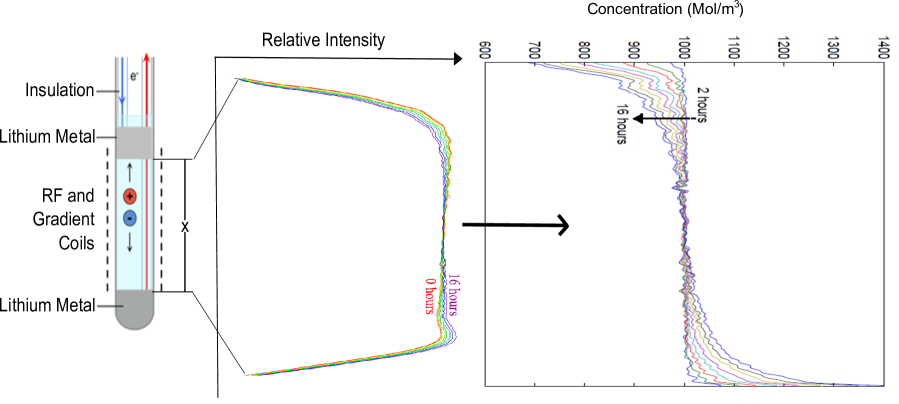
Figure 1: Experimental setup and the measured concentration data ${\tilde{c}}(x,t)$ used in the present study.

2.2 The Planck-Nernst Model

Here we recall the classical Planck-Nernst model used to describe the transport of charged species in dilute electrolytes [3]. The concentrations of cations and anions are denoted by $c_{+}$ and $c_{-}$ respectively. We make the following modelling assumptions in order to obtain the mathematical description of the mass transport during the galvanostatic experiment described in Section 2.1 [11]:

• isothermal conditions;

• the driving force for mass transport of a species is the gradient of its chemical potential;

• the lack of thermodynamic ideality (i.e., activity coefficient different from one) and the effect of the solution viscosity accounted for by an a priori undetermined dependence of the material properties on the salt concentration;

• ion transport occurs only in the axial direction and transport in the radial direction of the cell is negligible;

• the electrolyte solution is homogeneous at the beginning of the experiment;

• the system satisfies local electrical neutrality at every location in the bulk, which implies that $c_{+}=c_{-}=c$, were c is the salt concentration;

• mass transport occurs only by diffusion and migration in the applied electric field (i.e., convective transport is neglected);

• the cation flux at the two boundaries ($x$ = 0 and $x$ = $L$) corresponds to the applied electric current and results in lithium deposition and stripping, respectively [22, 3].

We therefore consider a 1D problem with the spatial coordinate $x\in[0,L]$, where $L$ is the length of the electrolyte filled region in the cell, and time $t\in[0,T]$, where $T$ denotes the duration of the experiment. The above assumptions lead to the following partial differential equation (PDE) describing mass transport in the electrolyte solution (1a), subject to the boundary conditions (1b) and the initial condition (1c):

$$\frac{\partial c}{\partial t} =\frac{\partial}{\partial x}\left[{D}\frac{\partial c}{\partial x}+\frac{\left(1-{t^{+}}\right)I}{FA}\right] \text{in}\ (0,L)\times(0,T],$$ (1a)

$$\left.\frac{\partial c}{\partial x}\right|_{x=0,L} =-\frac{\left(1-{t^{+}}\right)I}{{D}FA} \text{in}\ (0,T],$$ (1b)

$$\left.c\right|_{t=0} =c^{\text{init}} \text{in}\ (0,L),$$ (1c)

where $c^{\text{init}}$ is the initial concentration, $A$ is the cross-sectional area of the cell, $F$ is Faraday’s constant, whereas $I$ denotes the applied constant current. We note that the effective Fickian diffusion coefficient $D$ and the transference number $t^{+}$ are considered unknown and will be reconstructed from the experimental data using the inverse modelling approach described in the following subsection. In the standard Planck-Nernst theory, both the diffusion coefficient $D$ and the transference number $t^{+}$ are assumed constant. In addition to this formulation, we will also consider a more general set-up with the diffusion coefficient and the transference number depending on the concentration, i.e., $D=D(c)$ and $t^{+}=t^{+}(c)$, which accounts for the thermodynamic non-ideality of the electrolyte solution. To simplify our notation, we will denote the pair of unknown material properties $m$, regardless of whether these properties are constant ($m=[D,t^{+}]$), or concentration-dependent ($m=[D(c),t^{+}(c)]$). The solutions of system (1) then define a map ${\mathcal{L}}$ from the material properties $m$ to the space- and time-dependent concentrations, i.e.,

$$c(x,t;m)={\mathcal{L}}(m),\qquad 0\leq x\leq L,\ 0\leq t\leq T.$$ (2)

2.3 Inverse Modeling

The unknown material properties, $D$ and $t^{+}$, can be reconstructed based on the assumed transport model (1) using the concentration profiles obtained in the NMR experiment described in Section 2.1. We will use the deterministic inverse modelling approach developed and validated in [11] in which the problem is framed as minimization of an error functional representing the least-squares deviation between the concentration values $c$ predicted by model (1) for a given set of material properties $m$ and the experimentally determined concentration values $\tilde{c}$. The error functional can thus be represented as

$$\mathcal{J}(m)=\frac{1}{2}\sum_{i=0}^{N_{T}}\int_{0}^{L}\left[c(x,t_{i};m)-\tilde{c}(x,t_{i})\right]^{2}\,dx,$$ (3)

where $N_{T}$ is the number of time levels $t_{i}$ where the concentration profiles are acquired during the experiment. We will consider two distinct formulations corresponding, respectively, to constant and to concentration-dependent material properties.

When both $D$ and $t^{+}$ are constant, we obtain a simple unconstrained optimization problem (which is exact in the limiting case of an ideal solution, i.e., at very dilute salt concentrations)

$$\text{P1}:\qquad[\widehat{D},\widehat{t}^{+}]=\operatorname*{\arg\!\min}\limits_{[t^{+},D]\in\mathbb{R}^{2}}\mathcal{J}([D,t^{+}])$$

(henceforth carets “$\widehat{\cdot}$” will denote optimal reconstructions). Problem P1 can be solved in a straightforward manner using commercially available software tools such as the minimization routines in MATLAB. It was in fact already solved in the seminal study by Klett et al. [7] and is also solved here as a preliminary step in a more complete analysis.

A more complicated optimization problem arises when both $D(c)$ and $t^{+}(c)$ are concentration-dependent, which reflects the physics of the problem in more realistic fashion,

$$\text{P2}:\qquad[\widehat{D}(c),\widehat{t}^{+}(c)]=\operatorname*{\arg\!\min}\limits_{[t^{+}(c),\,D(c)]\in\mathcal{X}}\mathcal{J}\left([D(c),t^{+}(c)]\right),$$

where ${\mathcal{X}}$ denotes a suitable function space to which the pair $[D(c),t^{+}(c)]$ belongs. The functions $D(c)$ and $t^{+}(c)$ are defined on the interval $[c_{\alpha},c_{\beta}]$ bounded by some minimum and maximum concentrations $c_{\alpha}$ and $c_{\beta}$, respectively.

We emphasize that, apart from smoothness and the behavior at the endpoints (i.e., for $c\rightarrow c_{\alpha},c_{\beta}$), no other a priori assumptions are made about the functional forms of $D(c)$ and $t^{+}(c)$. In contrast to the simplified case (problem P1), the computational approach required to solve the more realistic case (problem P2) with concentration-dependent material properties is more involved and necessitates specialized tools. This approach has the general form of iterative gradient-based minimization

$$D^{(n+1)}(c) =D^{(n)}(c)-\xi_{D}^{(n)}\,\nabla_{D}\mathcal{J}\left(D^{(n)}(c),t^{+(n)}(c)\right) n=1,2,\dots,$$ (4a)

$$t^{+(n+1)}(c) =t^{+(n)}(c)-\xi_{t^{+}}^{(n)}\,\nabla_{t^{+}}\mathcal{J}\left(D^{(n+1)}(c),t^{+(n)}(c)\right) n=1,2,\dots,$$ (4b)

$$[D^{(1)}(c),t^{+(1)}(c)] =[\widehat{D},\widehat{t}^{+}],$$ (4c)

where $\nabla_{D}\mathcal{J}$ and $\nabla_{t^{+}}\mathcal{J}$ are the gradients (sensitivities) of error functional (3) with respect to perturbations of, respectively, $D(c)$ and $t^{+}(c)$, whereas $\xi_{D}^{(n)}$ and $\xi_{t^{+}}^{(n)}$ are the corresponding lengths of the descent steps in the two directions. The initial guess for problem P2 in (4c) is given by the constant values $\widehat{D}$ and $\widehat{t^{+}}$ which are the optimal reconstructions obtained from problem P1. (Problem P1 also requires an initial guess, however, this problem tends to have a unique minimum and therefore this initial guess may be arbitrary [23]. Thus, the advantage of solving problem P1 first is that it provides a very robust initial guess for problem P2.) The optimal concentration-dependent properties can then be computed using (4) as $\widehat{D}(c)=\lim_{n\rightarrow\infty}D^{(n)}(c)$ and $\widehat{t^{+}}(c)=\lim_{n\rightarrow\infty}t^{+(n)}(c)$. A key element of the iterative process (4) is the evaluation of error functional gradients $\nabla_{D}\mathcal{J}$ and $\nabla_{t^{+}}\mathcal{J}$ for which details are provided in A. We also refer the reader to [24, 25] for a discussion of further mathematical and computational details of this approach.

The estimates of the material properties obtained by solving problems P1 and P2 are optimal, in the sense of minimizing the error with respect to measurements, cf. (3). Such inverse problems are however known to be often “ill-posed”, meaning that the presence of noise in the measurement data may significantly affect the reconstructed solution [9, 4]. The sensitivity of the obtained reconstructions to perturbations of the data may be probed by performing a Monte-Carlo analysis [11] in which problems P1 and P2 are solved repeatedly using measurements $\tilde{c}$ artificially contaminated with independent noise samples with an assumed (e.g., normal) distribution and magnitude determined by the known size of the measurement errors. While this approach provides valuable insights about the sensitivity of the reconstructed material properties to noise in the data, it does not quantify their uncertainty in the sense of indicating which values of the material properties are most likely. A solution to this problem is presented in the next subsection.

2.4 Bayesian Approach to Uncertainty Quantification

We assume here that both the measurements $\tilde{c}(x,t)$ and the reconstructed material properties $[D,t^{+}]$, or $[D(c),t^{+}(c)]$, are random variables characterized by certain probability density functions (PDFs). More precisely, in the case of concentration-dependent properties, $D(c)$ and $t^{+}(c)$ are given by suitable probability distributions for all concentration values $c\in[c_{\alpha},c_{\beta}]$ and the same also applies to the measurements $\tilde{c}$ for different values of $x\in[-0,L]$ and $t\in[0,T]$.

In the Bayesian framework, the probability distribution of the reconstructed material properties is given in terms of the posterior probability ${\mathbb{P}}(m|{\tilde{c}})$, which is the probability of $m$ attaining a certain value (in problem P2, for a given concentration $c$) given observations ${\tilde{c}}$, and can be expressed using Bayes’ rule [14, 12, 13]

$${\mathbb{P}}(m|{\tilde{c}})=\frac{{\mathbb{P}}({\tilde{c}}|m)\,{\mathbb{P}}(m)}{{\mathbb{P}}({\tilde{c}})},$$ (5)

where ${\mathbb{P}}(m)$ is the prior distribution reflecting our a priori assumptions about the solution, ${\mathbb{P}}({\tilde{c}}|m)$ is the likelihood of observing particular experimental data for a given set of material properties, whereas ${\mathbb{P}}({\tilde{c}})$ is a normalizing factor.

In terms of the prior distribution ${\mathbb{P}}(m)$, one can take the distribution of $m$ obtained by performing a Monte-Carlo sensitivity analysis of the deterministic inverse problems P1 and P2, as described at the end of section 2.3. This is accomplished by solving problems P1 and P2 $N\geq 1$ times, each time using the original measurements ${\tilde{c}}$ perturbed with normally-distributed noise with magnitude given by the known size of experimental errors. The obtained material properties $m$ are then used to construct the prior distribution ${\mathbb{P}}(m)$. This step appears as STAGE 1 in Algorithms 1 and 2 below. We note that this analysis does not account for how good the fits are, in terms of the value of the error functional (3), for various samples of the noise perturbing the measurements. A alternative, neutral, approach would be to take “uninformative” priors given by uniform distributions of $m$.

As regards the likelihood function, the following ansatz is typically adopted in Bayesian inference [14, 12, 13]

$${\mathbb{P}}({\tilde{c}}|m)\propto e^{-{\mathcal{J}}(m)},$$ (6)

which expresses the assumption that for a given set of material properties $m$, measurements resulting in large values of the error functional (3) are less likely to be observed. The likelihood function ${\mathbb{P}}({\tilde{c}}|m)$ is approximated by sampling the distribution in (6) using the Metropolis-Hastings algorithm [26] to produce $M$ samples. This algorithm is based on the Markov-Chain Monte-Carlo (MCMC) approach [27] employed to randomize $m$ and at each step involves solution of the governing system (1) for modified (trial) material properties $m^{*}$ followed by the evaluation of the error functional (3). At each step the algorithm moves in the probability space collecting samples from the probability distribution (5). A move in the probability space is accepted or rejected based on a sample acceptance ratio $\gamma$ defined based on the posterior distribution (5) (see Algorithm 1 and 2). If one attempts to move to a point in the probability space that is more probable than the existing point, the move is accepted. On the other hand, if one attempts to move to a less probable point, the algorithm reject the move with some probability based on the steepness of the probability decrease in the given direction. Thus, the trajectory tends to sample frequently from high-probability regions while occasionally also sampling from low-probability regions. The MCMC algorithm involves a “burn-in” process in which a certain number (usually the first $10\%$) of the total number $M$ of accepted samples is discarded to avoid outliers common at initial stages.

While application of the Metropolis-Hastings algorithm is fairly straightforward in the finite-dimensional setting of problem P1, it is more delicate in the continuous setting of problem P2. The main difficulty is in constructing random perturbations of the concentration-dependent material properties $D(c)$ and $t^{+}(c)$ in a way that they will remain smooth enough for the Planck-Nernst system (1) to be well defined (normally, these functions should be at least once continuously differentiable and this issue is also addressed at the end of A). This is achieved by parameterizing the material properties in terms of their truncated cosine-series representations

$$m_{P}(c) =\frac{\hat{m}_{0}}{2}+\sum_{k=1}^{P}\hat{m}_{k}\cos\left[\frac{2\pi k(c-c_{\alpha})}{c_{\beta}-c_{\alpha}}\right],\quad c\in[c_{\alpha},c_{\beta}]$$ (7)

$$\text{where}\quad\hat{m}_{k} =\frac{2}{c_{\beta}-c_{\alpha}}\int_{c_{\alpha}}^{c_{\beta}}m(c)\cos\left[\frac{2\pi k(c-c_{\alpha})}{c_{\beta}-c_{\alpha}}\right]\,dc,\quad k=1,\dots,P$$

and the number of terms $P$ is a discretization parameter. The choice of the cosine-series expansion is dictated by the assumed behavior of $D(c)$ and $t^{+}(c)$ at $c=c_{\alpha},c_{\beta}$. The Metropolis-Hastings algorithm is initialized with a function $m_{P}(c)$ for which the cosine-series coefficients in (7) vanish as $|\hat{m}_{k}|\sim\mathcal{O}(k^{-2})$. New trial samples are generated by multiplying the cosine-series coefficients $\hat{m}_{1},\dots,\hat{m}_{P}$ by independent random numbers $\eta_{k}$, $k=1,\dots,P$, chosen such that $|\eta_{k}|<C$ for all $k$, where $C>0$ is a parameter. For sufficiently large $P$ this approach approximates a continuous random distribution while preserving the required smoothness of the trial material properties $[D(c),t^{+}(c)]$. The proposed computational approach for Bayesian uncertainty quantification is summarized as Algorithms 1 and 2 for the problems with constant and concentration-dependent material properties, respectively, and is validated in the next section.

We note that, somewhat unconventionally, both the $prior$ distribution and the $likelihood$ function are derived here from the same experimental data, albeit in fundamentally different ways. In the absence of other possibilities, an alternative solution would be to use an uninformative prior. However, the proposed approach is preferred as it results in tighter bounds.

  STAGE 1: Construct $N$ samples for prior distribution ${\mathbb{P}}(m)$

  repeat

     perturb measurements ${\tilde{c}}$ with normally-distributed noise (magnitude given by the size of experimental errors)

     find $\widehat{m}$ by solving problem P1 (using function fminsearch and initial guess $m^{(0)}$)

     store $\widehat{m}$ as a sample for prior distribution

  until $N$ prior distribution samples are obtained

  assimilate samples to construct $\mathbb{P}(\bar{m})$

  

  STAGE 2: Construct $M$ samples for posterior distribution ${\mathbb{P}}(m|{\tilde{c}})$

  construct initial sample $\bar{m}^{(0)}$

  $k\leftarrow 1$

  repeat

     create a new trial position $\bar{m}^{*}=\bar{m}^{k}+\texttt{normrnd}(\bar{0},C)$

     calculate acceptance ratio $\gamma=\frac{\mathbb{P}(\bar{m}^{(*)}|{\tilde{c}})}{\mathbb{P}(\bar{m}^{(k)}|{\tilde{c}})}$

     if $\gamma\geq\texttt{rand}(1)$:  $\bar{m}^{(k+1)}$=$\bar{m}^{(*)}$;  $k\leftarrow k+1$,

     else:       discard $m^{(*)}$

     $k=k+1$

  until $M+M/10$ samples are obtained for posterior distribution

  discard the first $M/10$ samples

  assimilate the remaining samples to construct posterior probability distribution ${\mathbb{P}}(m|{\tilde{c}})$

Algorithm 1 : Two-stage algorithm to estimate the posterior probability distribution of constant material properties (normrnd and fminsearch are MATLAB functions).
Input:
    ${\tilde{c}}$ — experimental data,
    $N,M$ — numbers of samples generated in STAGE 1 and STAGE 2
    $\varepsilon_{{\mathcal{J}}}$ — tolerance in the solution of problem P1 in STAGE 1
    $m^{(0)}$ — initial guess in the solution of problem P1 in STAGE 1
    $\bar{m}^{(0)}$ — initial guess sample in STAGE 2
    $C$ — parameter controlling randomization in in STAGE 2
Output:
    an approximation of the posterior probability distribution ${\mathbb{P}}(m|{\tilde{c}})$

  STAGE 1: Construct N samples for prior distribution of $\mathbb{P}(\bar{m})$

  repeat

     perturb measurements ${\tilde{c}}$ with normally-distributed noise (magnitude given by the size of experimental errors)

     $\bar{m}^{(0)}\leftarrow\hat{m}$ (initial guess)

     $n\leftarrow 1$

     repeat

        solve governing system (2)

        evaluate $\nabla_{\bar{m}}\mathcal{J}$.

        compute the conjugate direction $\mathbf{g}\left[\nabla_{\bar{m}}\mathcal{J}\right]$

        perform line minimization: $\tau^{(n-1)}_{\bar{m}}$ $\leftarrow$ $\operatorname*{\arg\!\min}\limits_{\tau}\left\{\mathcal{J}\left({\bar{m}}^{(n-1)}-\tau\,\mathbf{g}\left[\nabla_{\bar{m}}\mathcal{J}\right],\right)\right\}$

        update: $\bar{m}^{(n)}\ \leftarrow\ \bar{m}^{(n-1)}-\tau^{(n-1)}_{\bar{m}}\,\mathbf{g}\left[\nabla_{\bar{m}}\mathcal{J}\right]$

        $n\leftarrow n+1$

     until $|\mathcal{J}(\bar{m}^{(n)})-\mathcal{J}(\bar{m}^{(n-1)})|<\,\varepsilon_{\mathcal{J}}|\mathcal{J}(\bar{m}^{(n)}|$

     store $\bar{m}^{(n)}$ as prior distribution sample

  until N prior distribution samples are obtained

  assimilate samples to construct $\mathbb{P}(\bar{m})$.

  STAGE 2: Construct M samples for posterior distribution $\mathbb{P}(\bar{m}|{\tilde{c}})$

  $\bar{m}^{(0)}\leftarrow\bar{m}^{i}$

  $k\leftarrow 1$

  repeat

     create a new trial position $\bar{f}^{*}=\bar{f}^{k}\times\texttt{normrnd}(\bar{0},C)$

     using inverse Fourier transform obtain $\bar{m}^{(*)}$

     calculate acceptance ratio $\gamma=\frac{\mathbb{P}(\bar{m}^{(*)}|{\tilde{c}})}{\mathbb{P}(\bar{m}^{(k)}|{\tilde{c}})}$

     if $\gamma\geq\texttt{rand}(1)$:  $\bar{m}^{(k+1)}$=$\bar{m}^{(*)}$;  $k\leftarrow k+1$,

     else:       discard $\bar{m}^{(*)}$

  until M+M/10 samples are obtained for posterior distribution

  discard the first $M/10$ samples

  assimilate the remaining samples to obtain posterior probability distribution

Algorithm 2 : Two-stage algorithm to estimate the posterior probability distribution of constant material properties (normrnd and fminsearch are MATLAB functions).
Input:
    ${\tilde{c}}$ — experimental data,
    $N,M$ — numbers of samples generated in STAGE 1 and STAGE 2
    $\varepsilon_{{\mathcal{J}}}$ — tolerance in the solution of problem P2 in STAGE 1
    $\hat{m}$ — initial guess in the solution of problem P2 in STAGE 1, (here the solution of problem P1 is used as $\hat{m}$)
    $\bar{m}^{i}$ — initial sample in STAGE 2 (chosen such that $\bar{m}^{i}\in{\mathcal{X}}$)
    $C$ — parameter controlling randomization in in STAGE 2
Output:
    an approximation of the posterior probability distribution ${\mathbb{P}}(m|{\tilde{c}})$

3 RESULTS

3.1 Validation

In this section we validate the Bayesian approach to uncertainty quantification introduced in Section 2.4. In addition to establishing its consistency, this will also allow us to assess how the results it produces depend on key numerical parameters and properties of the data. We will do this for both problems P1 and P2 using an approach based on “manufactured solutions” [24, 25], where certain values of $D$ and $t^{+}$ (in problem P1), or functional forms of $D(c)$ and $t^{+}(c)$ (in problem P2), are initially assumed and used to generate ”measurements” by solving system (1). After being contaminated with noise of prescribed magnitude, this data is used to solve inverse problems P1 and P2 and then to quantify the uncertainty of the obtained reconstructions using Algorithms 1 and 2. In particular, this approach allows one to determine how the uncertainty of the reconstructions depends on the level of noise in the data.

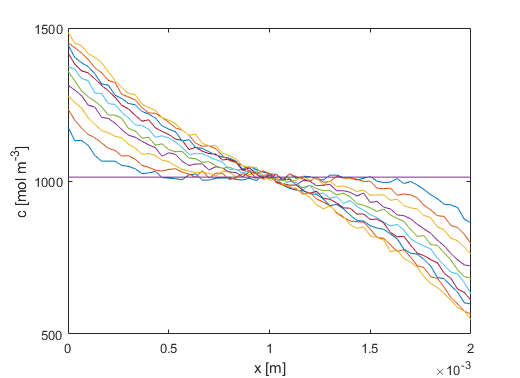
(a)

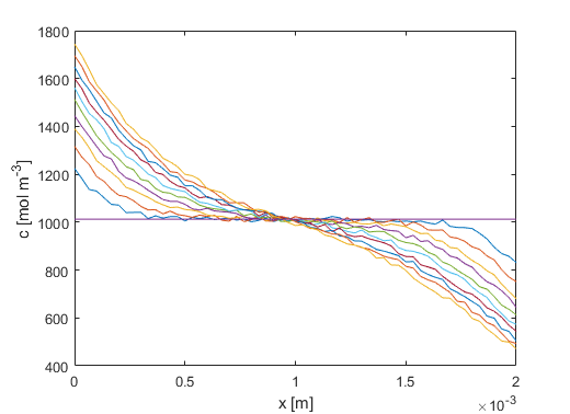
(b)

Figure 2: Concentration profiles ${\tilde{c}}(x,t_{i})$, $i=1,\dots,N_{T}$, manufactured by solving problem (1) using (a) assumed constant material properties $[D,t^{+}]$ and (b) assumed concentration-dependent material properties $[D(c),t^{+}(c)]$. In both cases the added noise has variance $\xi=25$ mol m^-3.

For problem P1 we assume $D=10^{-10}$ m²s^-1 and $t^{+}=0.4$, whereas the assumed functional forms of $D(c)$ and $t^{+}(c)$ in problem P2 are shown with thick dashed lines in Figures 5a and 5b, respectively. We also assume that the electrochemical cell has length $L=0.002$ m and diameter $0.001$ m, the applied current is $I=100$ $\mu$A and the initial salt concentration is $c^{\text{init}}=1000$ mol m^-3, whereas the duration of the experiment is $T=20$ hours, all of which are in the ballpark of parameters used in practice. System (1) and its adjoint (19) are solved numerically in MATLAB with the routine pdepe which uses adaptive spatial discretization and adaptive time-stepping adjusted such that the relative and absolute tolerances, respectively, $10^{-8}$ and $10^{-10}$ are satisfied at all points in time and space. Computed concentration profiles recorded at $N_{T}=10$ equispaced time levels $t_{i}$, $i=1,\dots,N_{T}$, are used as the measurements ${\tilde{c}}(x,t_{i})$ (the integral with respect to time $t$ in (3) is therefore replaced with summation over $i=1,\dots,N_{T}$). Thus generated measurements are then perturbed with normally-distributed noise with the frequency 20 kHz and variance $\xi=25$ mol m^-3. The concentration profiles ${\tilde{c}}(x,t_{i})$, $i=1,\dots,N_{T}$, obtained with constant $[D,t^{+}]$ and concentration-dependent material properties $[D(c),t^{+}(c)]$ are shown in Figures 2a and 2b, respectively. When sampling the likelihood function ${\mathbb{P}}({\tilde{c}}|m)$ in Algorithm 2 expression (7) is used with $P=50$ terms.

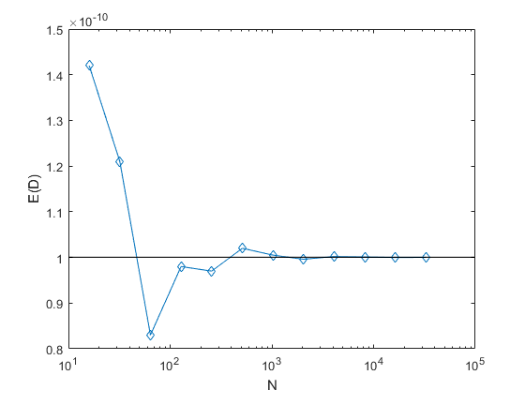
(a)

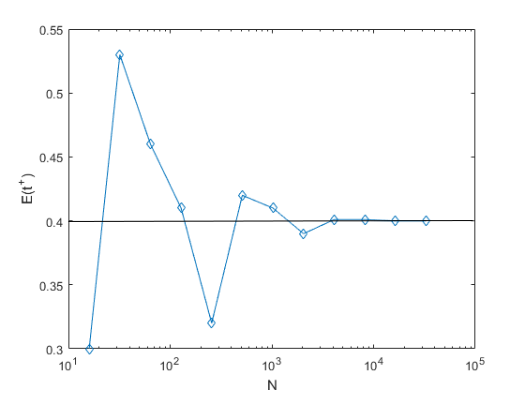
(b)

Figure 3: Convergence of the expected (constant) values of (a) $D$ and (b) $t^{+}$ to the true values indicated with horizontal lines as the number of samples $N$ and $M=N$ used in Algorithm 1 is increased. Measurement data is available at $N_{T}=10$ time levels and the noise variance is $\xi=25$ mol m^-3.

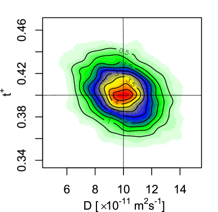
Figure 4: Joint posterior probability distribution of the constant diffusion coefficient $D$ and transference number $t^{+}$. Measurement data is available at $N_{T}=10$ time levels and the noise variance is $\xi=25$ mol m^-3.

We begin the presentation of the results by analyzing the effect of the number of samples used to approximate the prior probability distribution and the likelihood function ${\mathbb{P}}({\tilde{c}}|m)$ on the convergence of the expected values of the constant material properties in Figure 3. For simplicity, we set $M=N$ in Algorithm 1. In Figures 3a and 3b we see that as the number of Monte-Carlo samples $N$ increases the expected values of $D$ and $t^{+}$, estimated based on the posterior probability distributions ${\mathbb{P}}(m|{\tilde{c}})$ produced by Algorithm 1, converge to their true values. Acceptable accuracy is achieved already for $N=5,000$ and this is the number of samples we will use below. Next, in Figure 4, we present the joint probability density of the constant material properties $D$ and $t^{+}$ based on the posterior distributions obtained with Algorithm 1. The approximately symmetric shape of the isolines in this figure indicates that there is no significant correlation between the uncertainties in the reconstruction of the diffusion coefficient and the transference number. The corresponding results obtained with Algorithm 2 for the problem with concentration-dependent material properties are presented in Figures 5a and 5b for $D(c)$ and $t^{+}(c)$, respectively, together with the corresponding true distributions. The contour plots shown in these figures should be interpreted such that their sections at a given value of $c$ produce the posterior probability distributions functions ${\mathbb{P}}(D(c)|{\tilde{c}})$ and ${\mathbb{P}}(t^{+}(c)|{\tilde{c}})$. We observe that, unlike in Figure 5b where the most likely values of the transference number $t^{+}(c)$ are quite close to the true distribution for all values of $c$, in Figure 5a a systematic difference between the most likely reconstructed values of $D(c)$ and the true values is evident. We remark here that in the absence of noise in the data, the concentration-dependent diffusion coefficient $D(c)$ obtained by solving problem P2 is inferred very accurately and coincides with the true distribution up to the graphical resolution for all values of $c$ (this result is not shown). Hence, we can conclude that the differences evident in Figure 5a are induced by noise and as such can be attributed to the ill-posedness of the inverse problem (cf. the discussion in Introduction).

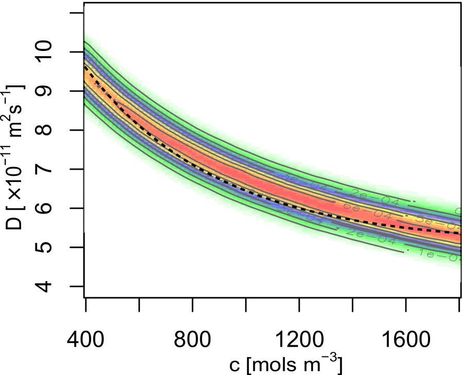
(a)

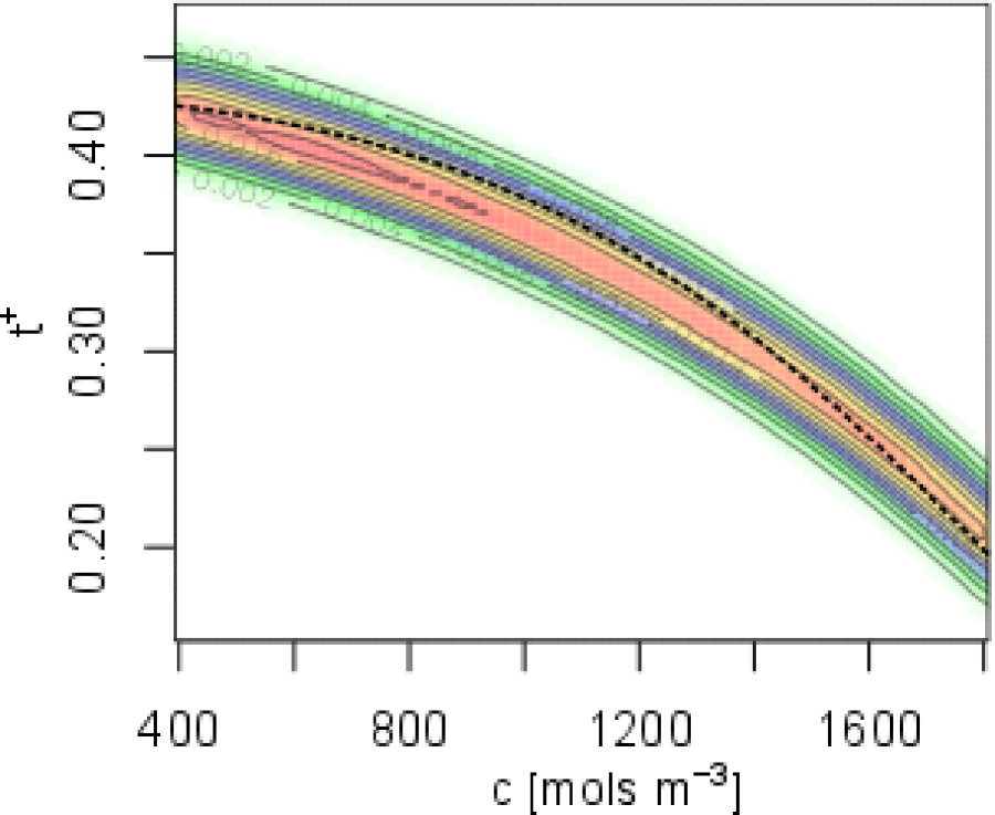
(b)

Figure 5: Posterior probability densities of (a) the diffusion coefficient $D(c)$ and (b) the transference number $t^{+}(c)$ as functions of the concentration $c$. Measurement data is available at $N_{T}=10$ time levels and the noise variance is $\xi=25$ mol m^-3. The thick dashed lines represent the true distributions of $D(c)$ and $t^{+}(c)$.

We now move on to characterize the impact of the noise level in the data ${\tilde{c}}$ on the uncertainty of the reconstructed material properties. This is done by using noise with three different variances $\xi=25,50,75$ mol m^-3 and computing the posterior distribution of the constant and concentration-dependent material properties, $[D,t^{+}]$ and $[D(c),t^{+}(c)]$, using Algorithms 1 and 2. The results are presented, respectively, in Figures 6a and 7, where they are shown in terms of the $95\%$ confidence bounds defined as the boundaries of parameter regions over which the posterior probability density integrates to $0.95$. We observe in these figures that the confidence regions corresponding to different noise levels have similar shapes and in all cases shrink as the noise level is reduced, which is the expected behavior.

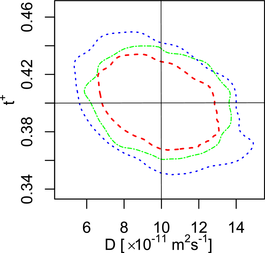
(a)

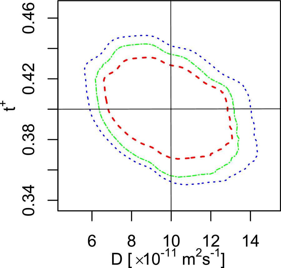
(b)

Figure 6: Boundaries of the $95\%$ confidence regions in the joint posterior probability distributions of the constant diffusion coefficient $D$ and transference number $t^{+}$ obtained with (a) concentration profiles ${\tilde{c}}(x,t_{i})$ available at $N_{T}=10$ time levels and perturbed with noise of different magnitudes (dashed — $\xi=25$ mol m^-3, dot-dash — $\xi=50$ mol m^-3, dotted — $\xi=75$ mol m^-3) , (b) concentration profiles ${\tilde{c}}(x,t_{i})$ available at different numbers of time levels (dashed — $N_{T}=10$, dot-dash — $N_{T}=7$, dotted — $N_{T}=4$) and perturbed with noise of magnitude $\xi=25$ mol m^-3.

We close this section by analyzing the effect of the amount of available measurement data on the uncertainty of the reconstructed material properties. This is done by varying the number $N_{T}$ of the time levels $t_{i}$ where measurements ${\tilde{c}}(x,t_{i})$, $i=1,\dots,N_{T}$, are available ($N_{T}=4,7,10$) while keeping the noise variance fixed at $\xi=25$ mol m^-3. The results obtained for problems with constant and concentration-dependent material properties, $[D,t^{+}]$ and $[D(c),t^{+}(c)]$, are presented, respectively, in Figures 6b and 8, again using the $95\%$ confidence bounds for the posterior probability distributions determined with Algorithms 1 and 2. We can conclude from these figures that the effect of reducing the amount of available data is qualitatively similar to the effect of increasing the noise level in the data, as the uncertainty grows when $N_{T}$ is decreased.

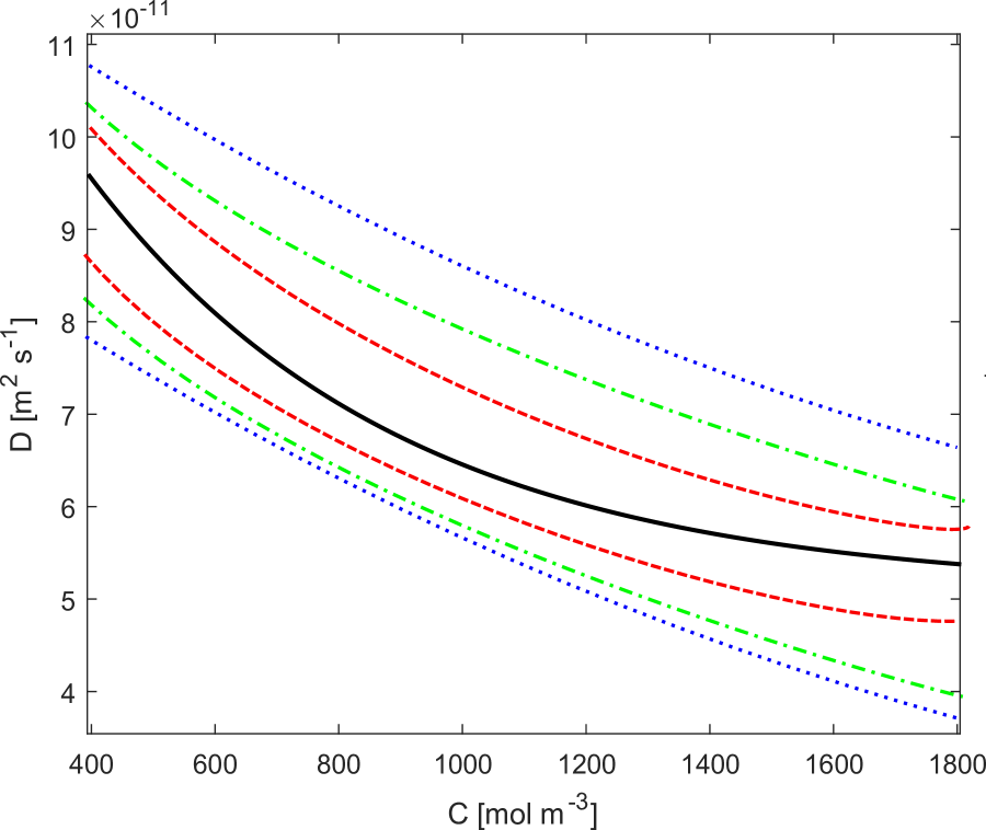
(a)

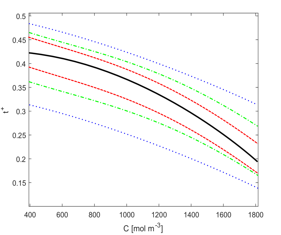
(b)

Figure 7: Boundaries of the $95\%$ confidence regions in the posterior probability distributions of (a) the diffusion coefficient $D(c)$ and (b) the transference number $t^{+}(c)$ for different concentration values. The results are obtained using concentration profiles ${\tilde{c}}(x,t_{i})$ available at $N_{T}=10$ time levels and perturbed with noise of different magnitudes (dashed — $\xi=25$ mol m^-3, dot-dash — $\xi=50$ mol m^-3, dotted — $\xi=75$ mol m^-3). The thick solid lines represent the true distributions of $D(c)$ and $t^{+}(c)$.

(a)

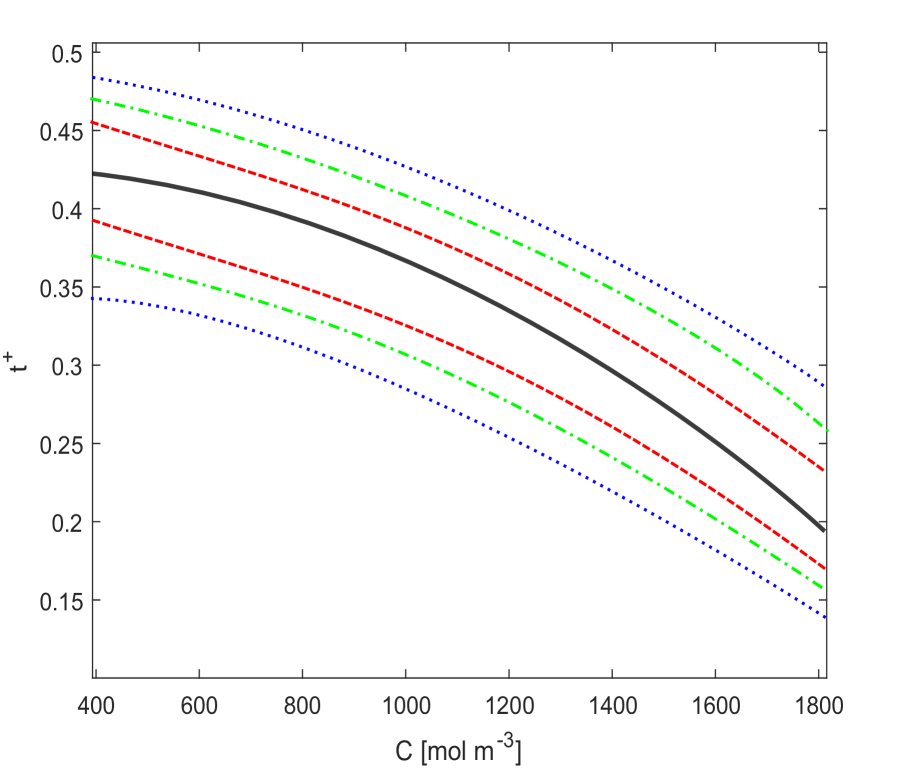
(b)

Figure 8: Boundaries of the $95\%$ confidence regions in the posterior probability distributions of (a) the diffusion coefficient $D(c)$ and (b) the transference number $t^{+}(c)$ for different concentration values. The results are obtained using concentration profiles ${\tilde{c}}(x,t_{i})$ available at different numbers of time levels (dashed — $N_{T}=10$, dot-dash — $N_{T}=7$, dotted — $N_{T}=4$) and perturbed with noise of magnitude $\xi=25$ mol m^-3. The thick solid lines represent the true distributions of $D(c)$ and $t^{+}(c)$.

3.2 Application to Experimental Data

In this section we apply the methodology for uncertainty quantification described in Section 2.4 and validated in Section 3.1 to the inverse problems P1 and P2 involving, respectively, constant and concentration-dependent material properties and using the experimental data described in Section 2.1. The joint posterior probability density obtained for constant $[D,t^{+}]$ is shown in Figure 9a, whereas the posterior probability densities of $D(c)$ and $t^{+}(c)$ as functions of the concentrations $c$ are shown in Figures 9b and 9c. In addition, in Figures 10a–10c we also present the joint posterior probability densities of $[D(c),t^{+}(c)]$ for three selected concentration values (these distributions are extracted from the data in Figures 9b and 9c by constructing sections at the indicated values of $c$).

First, in Figure 9 we note that the expected values of both constant and concentration-dependent material properties as well as the trends with changes of the concentration revealed in the latter case agree with the results known from the literature [11]. In Figure 9a we also observe that the reconstructed constant material properties exhibit significant uncertainties which, unlike the validation results from Figure 4, are correlated in the sense that larger values of the diffusion coefficient $D$ are likely to occur together with smaller values of the transference number $t^{+}$, and vice versa. On the other hand, in the concentration-dependent case the reconstruction uncertainty is significantly reduced for both $D(c)$ and $t^{+}(c)$ for all concentration values $c$. In both cases this uncertainty is small relative to the variation of $D(c)$ and $t^{+}(c)$ over the entire range of $c$. Moreover, Figures 10a–10c demonstrates that, in contrast to the case of constant material properties, cf. Figure 9a, in the concentration-dependent case there is no significant correlation between the uncertainties of $D(c)$ and $t^{+}(c)$ at particular values of $c$.

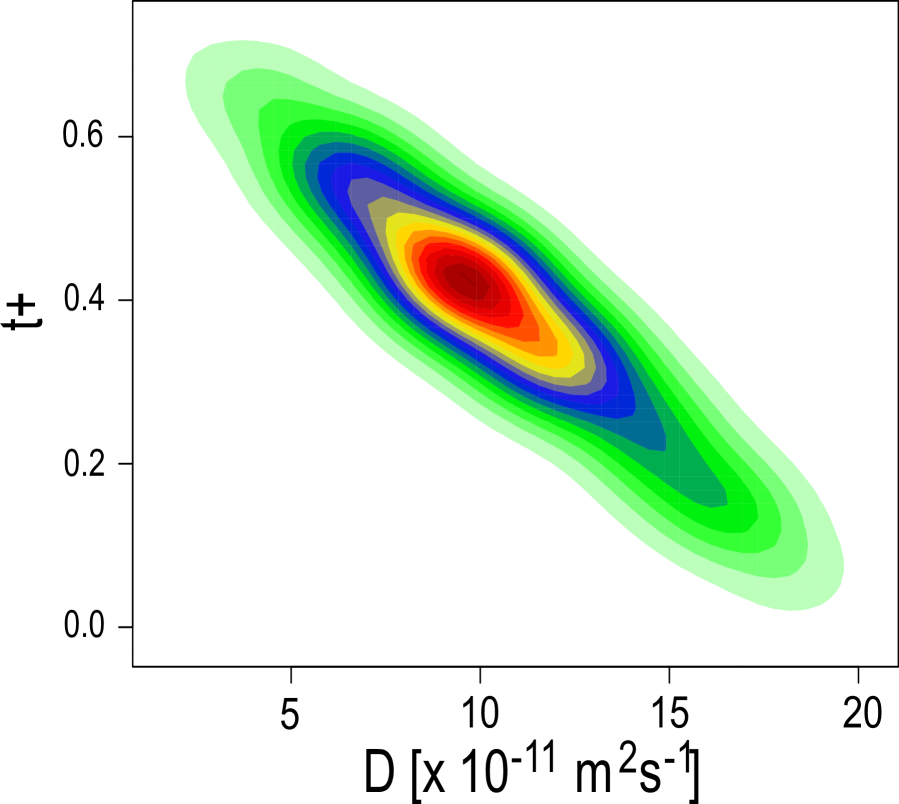
(a)

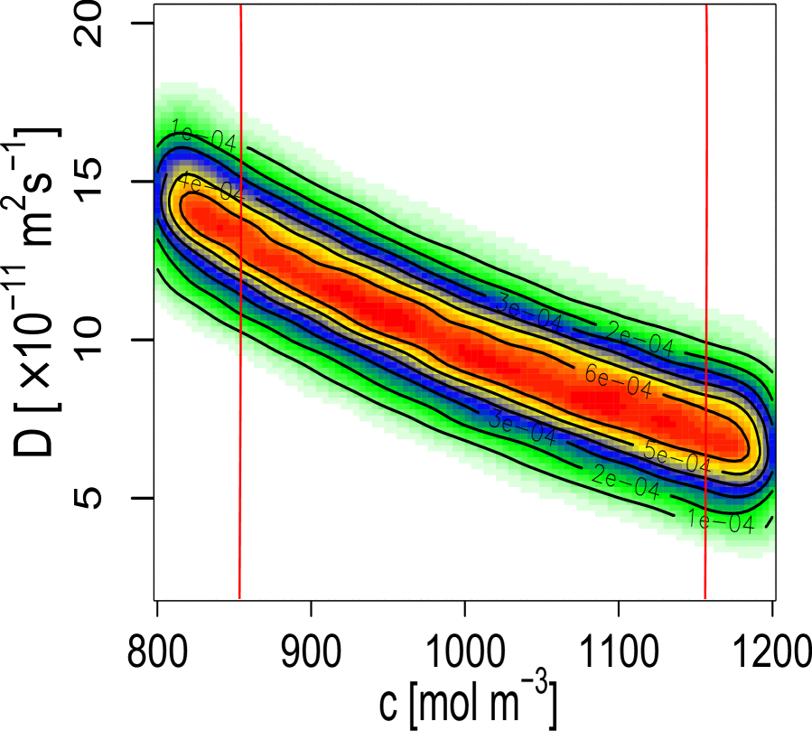
(b)

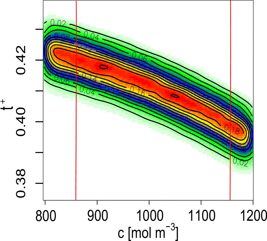
(c)

Figure 9: (a) Joint posterior probability distribution of the constant diffusion coefficient $D$ and transference number $t^{+}$, posterior probability densities of (b) the diffusion coefficient $D(c)$ and (c) the transference number $t^{+}(c)$ as functions of the concentration $c$, all obtained based on the measurement data described in Section 2.1.

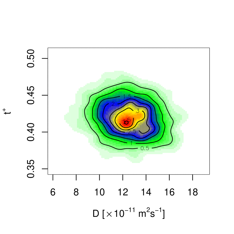
(a)

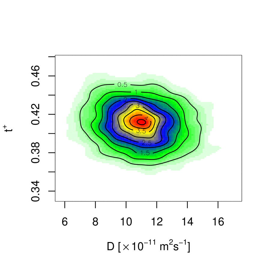
(b)

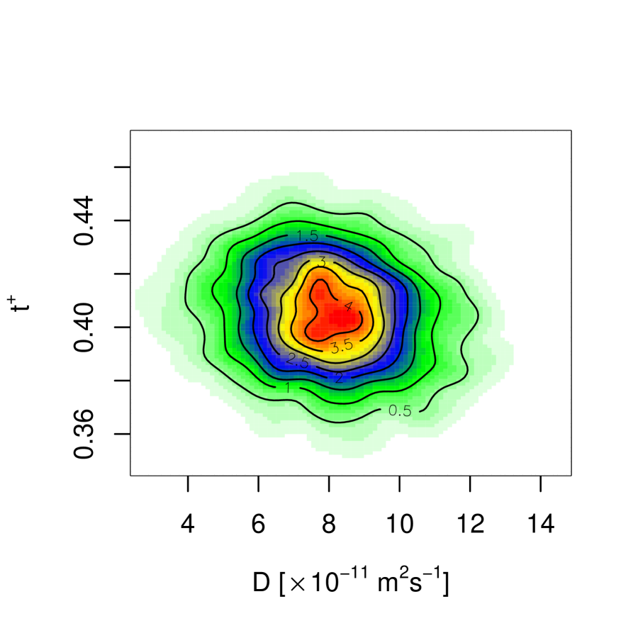
(c)

Figure 10: Joint posterior probability distribution of the concentration-dependent diffusion coefficient $D(c)$ and transference number $t^{+}(c)$ at the concentrations (a) $c=900$ mol m^-3, (b) $c=1,000$ mol m^-3 and (c) $c=1,100$ mol m^-3, cf. Figures 9b and 9c, obtained based on the measurement data described in Section 2.1.

4 CONCLUSIONS

In this study we have developed and carefully validated a state-of-the-art Bayesian approach to quantify the uncertainty of material properties reconstructed from experimental data. This approach combines a recently developed inverse-modelling technique capable of inferring general concentration-dependent material properties subject to minimal assumptions [11] with a Markov-Chain Monte-Carlo method for sampling the likelihood function. We emphasize that while the present study focuses on an electrochemical system modeled by the Planck-Nernst equation (1), the proposed approach is in fact also applicable to a broad range of problems in chemistry where macroscopic models are used. Extensive numerical tests of the method confirm that it exhibits the expected behavior as different parameters are varied.

Application of the proposed approach to actual experimental data allows us to place rigorous “error bounds” in the reconstructed material properties. These results demonstrate that while the uncertainty can be non-negligible for constant material properties, it is significantly reduced in the concentration-dependent case. The reason for this is that the required regularity of $D(c)$ and $t^{+}(c)$ as functions of $c$ (cf. the discussion at the end of A) imposes some constraints on how rapidly the material properties can vary with $c$. As a result, the reconstruction uncertainty is small relative to the range of variation of both $D(c)$ and $t^{+}(c)$, which offers confidence in the reliability of inverse modelling.

ACKNOWLEDGMENTS

The authors are thankful to J. M. Foster and I. Halalay for helpful discussions. Funding for this research was provided by an NSERC (Canada) Strategic Project Grant (# STPGP 479258-15).

Appendix A Error Functional Gradients

The gradients of the error functional (3) with respect to concentration-dependent properties $D(c)$ and $t^{+}(c)$ can be calculated starting from the directional derivatives defined as follows (to simplify the notation, we will not indicate the dependence on $c$ in this appendix)

$$\mathcal{J}^{\prime}([D,t^{+}];D^{\prime}) =\lim_{\epsilon\to 0}\epsilon^{-1}\left[\mathcal{J}([D+\epsilon D^{\prime},t^{+}])-\mathcal{J}([D,t^{+}])\right],$$ (8a)

$$\mathcal{J}^{\prime}([D,t^{+}];t^{{+^{\prime}}}) =\lim_{\epsilon\to 0}\epsilon^{-1}\left[\mathcal{J}([D,t^{+}+\epsilon t^{+^{\prime}}])-\mathcal{J}([D,t^{+}])\right],$$ (8b)

where $D^{\prime}$ and $t^{{+^{\prime}}}$ are the perturbations of control variables $D$ and $t^{+}$, respectively, and for simplicity of notation here and below we omit the dependence on $c$. In order to identify expressions for the gradients of the error functional as elements of a functional (Hilbert) space, we use the Riesz representation theorem [28]

$$\mathcal{J}^{\prime}([D,t^{+}];D^{\prime}) =\Big{\langle}\nabla_{D}\mathcal{J},D^{\prime}\Big{\rangle}_{\mathcal{X}},$$ (9a)

$$\mathcal{J}^{\prime}([D,t^{+}];t^{+^{\prime}}) =\Big{\langle}\nabla_{t^{+}}\mathcal{J},t^{+^{\prime}}\Big{\rangle}_{\mathcal{X}},$$ (9b)

where $\langle\cdot,\cdot\rangle_{\mathcal{X}}$ denotes the inner product in functional space $\mathcal{X}$ (to be specified below). To fix attention, we begin with the directional derivative (8a) with respect to the diffusion coefficient $D$ which can be evaluated as follows

$$\mathcal{J}^{\prime}([D,t^{+}];D^{\prime})=\sum_{i=1}^{N_{T}}\int_{0}^{T}\int_{0}^{L}\left[c(x,t;[D,t^{+}])-\tilde{c}(x,t)\right]\delta(t-t_{i})c^{\prime}(x,t;D,D^{\prime})\,dx\,dt,$$ (10)

where $\delta(\cdot)$ is the Dirac delta distribution and $c^{\prime}$ is the solution of the PDE system obtained as a perturbation of the governing system (1). Then, the following transformations is invoked

$$V(x,t)=\int_{c_{\alpha}}^{c(x,t)}D(s)\,ds,\quad x\in[0,L]\ \text{and}\ t\in[0,T],$$ (11)

where $c_{\alpha}=\min_{t\in[0,T],\;x\in[0,L]}c(x,t)$. We will define the identifiability interval ${\mathcal{I}}=[c_{\alpha},c_{\beta}]$, where $c_{\beta}=\max_{t\in[0,T],\;x\in[0,L]}c(x,t)$, as the range of concentration values spanned by solutions of (1). To simplify the notation, we also denote

$$Q(x,t)=\frac{(1-t^{+})I}{FA}.$$ (12)

Using these definitions, the perturbation system takes the form

$$\frac{\partial c^{\prime}}{\partial t} =\frac{\partial}{\partial x}\left(\frac{\partial V^{\prime}}{\partial x}+Q^{\prime}\right) \text{in}\ (0,L)\times(0,T],$$ (13a)

$$\left.\left(\frac{\partial V^{\prime}}{\partial x}+Q^{\prime}\right)\right|_{x=0,L} =0 \text{in}\ [0,T],$$ (13b)

$$\left.c^{\prime}\right|_{t=0} =0 \text{in}\ [0,L],$$ (13c)

where the perturbation variables $V^{\prime}$ and $Q^{\prime}$ are expressed as

$$V^{\prime}(x,t) =\int_{c_{\alpha}}^{c(x,t)}D^{\prime}(s)ds+D(c)c^{\prime}(x,t;D^{\prime}),$$ (14)

$$Q^{\prime}(x,t) =-\left[\left(V_{m}^{s}\right)\frac{dt^{+}}{dc}c^{\prime}(x,t;D^{\prime})+\right]\frac{I}{FA}.$$ (15)

We now observe that directional derivative (10) is not in a form consistent with Riesz representation (9a), because the perturbation variable $D^{\prime}$ does not appear explicitly in it, but is instead hidden (as $V^{\prime}$, cf. (14)) in the perturbation system (13). In order to transform the directional derivative (10) into the Riesz form (9a) we will employ adjoint analysis.

Multiplying equation (13a) by adjoint variable $c^{*}$ and integrating over the time and space domain, we get

$$\int_{0}^{L}\int_{0}^{T}\frac{\partial c^{\prime}}{\partial t}c^{*}\,dt\,dx=\int_{0}^{T}\int_{0}^{L}\left[\frac{\partial^{2}V^{\prime}}{\partial x^{2}}c^{*}+\frac{\partial Q^{\prime}}{\partial x}c^{*}\right]\,dx\,dt.$$ (16)

By re-organizing equation (16) and integrating it by parts with respect to both space and time we obtain

$$\int_{0}^{L}\left\{[c^{\prime}c^{*}]_{0}^{T}-\int_{0}^{T}\frac{\partial c^{*}}{\partial t}c^{\prime}dt\right\}\,dx\\ =\int_{0}^{T}\left\{\left[\frac{\partial V^{\prime}}{\partial x}c^{*}\right]_{0}^{L}-\int_{0}^{L}\frac{\partial V^{\prime}}{\partial x}\frac{\partial c^{*}}{\partial x}dx+[Q^{\prime}c^{*}]_{0}^{L}-\int_{0}^{L}Q^{\prime}\frac{\partial c^{*}}{\partial x}dx\right\}\,dt.$$ (17)

Using equations (13a)–(13c) we can eliminate a number of boundary terms after which we integrate the term with $\frac{\partial V^{\prime}}{\partial x}$ by parts one more time, so that we arrive at

$$\int_{0}^{L}\left\{[c^{\prime}c^{*}]_{t=T}-\int_{0}^{T}\frac{\partial c^{*}}{\partial t}c^{\prime}dt\right\}\,dx\\ =\int_{0}^{T}\left\{-\left[\frac{\partial c^{*}}{\partial x}V^{\prime}\right]_{0}^{L}+\int_{0}^{L}V^{\prime}\frac{\partial^{2}c^{*}}{\partial x^{2}}dx-\int_{0}^{L}Q^{\prime}\frac{\partial c^{*}}{\partial x}dx\right\}\,dt.$$ (18)

Now we assume that the adjoint system (defined on the same domain as the governing system (1)) is in the form

$$-\frac{\partial c^{*}}{\partial t} =D\frac{\partial^{2}c^{*}}{\partial x^{2}}+\frac{dt^{+}}{dc}\frac{I}{FA}\frac{\partial c^{*}}{\partial x}+\sum_{i=1}^{N_{T}}\left(c-\tilde{c}\right)\delta(t-t_{i}),$$ (19a)

$$\left.\frac{\partial c^{*}}{\partial x}\right|_{x=0,L} =0,$$ (19b)

$$\left.c^{*}\right|_{t=T} =0$$ (19c)

which reduces identity (18) to the following expression for the directional derivative of the error functional

$$\mathcal{J}^{\prime}([D,t^{+}];D^{\prime})=\int_{0}^{T}\int_{0}^{L}\left[\int_{c_{\alpha}}^{c(x,t)}D^{\prime}(s)ds\right]\frac{\partial^{2}c^{*}}{\partial x^{2}}\,dx\,dt.$$ (20)

We remark that adjoint system (19) is in fact a terminal value problem, cf. (19c), which means that it needs to be integrated backwards in time (however, since the term with the time derivative has a negative sign, the problem is well-posed). Although this is not the function space we will ultimately use in the computations, for now we set ${\mathcal{X}}=L^{2}({\mathcal{I}})$ meaning that our function space consists of square-integrable functions of the concentration $c$. The corresponding inner product, needed in (9a), is

$$\Big{\langle}\nabla_{D}^{L^{2}}{\mathcal{J}},D^{\prime}\Big{\rangle}_{L^{2}({\mathcal{I}})}=\int_{c_{\alpha}}^{c_{\beta}}\nabla_{D}{\mathcal{J}}(c)D^{\prime}(c)\,dc.$$ (21)

Changing the order of integration in (20) and employing (21) we arrive at the following expression for the $L^{2}$ gradient of the error functional

$$\nabla_{D}^{L^{2}}\mathcal{J}(s)=\int_{0}^{T}\int_{0}^{L}\chi_{\left[c_{\alpha},c(x,t)\right]}(s)\frac{\partial^{2}c^{*}}{\partial x^{2}}\,dx\,dt,\qquad s\in[c_{\alpha},c_{\beta}],$$ (22)

where $\chi_{\left[a,b\right]}=\begin{cases}1,\text{ }s\in\left[a,b\right]\\ 0,\text{ }s\notin\left[a,b\right]\end{cases}$.

Starting from the directional derivative (8b) and proceeding along the same lines as above we can derive an expression for the $L^{2}$ gradient of the error functional with respect to the concentration-dependent transference numbers

$$\nabla_{t^{+}}^{L^{2}}\mathcal{J}(s)=\int_{0}^{T}\int_{0}^{L}\frac{\partial c^{*}}{\partial x}\delta(s-c(x,t))\,dx\,dt,\qquad s\in[c_{\alpha},c_{\beta}],$$ (23)

where as before $c^{*}$ is a solution of adjoint system (19). Expressions (22) and (23) can be evaluated in a straightforward manner using standard numerical techniques.

Above we derived gradient expressions in the $L^{2}$ space, however, as pointed out in earlier studies [24, 25], such gradients are not suitable for the reconstruction of material properties, because they can potentially be discontinuous and undefined outside identifiability region $\mathcal{I}$. Therefore, in order to ensure suitable smoothness and domain of definition of the gradients, we will define them in the Sobolev space $H^{1}({\mathcal{I}})$ of functions of the concentration $c$ with square-integrable derivatives, i.e., in problem P2 we set ${\mathcal{X}}=H^{1}({\mathcal{I}})$. This space is characterized by the following inner product, cf. (9a)–(9b) (as we did above, we focus here on $\nabla_{D}\mathcal{J}$ with the transformation for $\nabla_{t^{+}}\mathcal{J}$ being analogous)

$$\Big{\langle}\nabla^{H^{1}}_{D}\mathcal{J},D^{\prime}\Big{\rangle}_{H^{1}({\mathcal{I}})}=\int_{c_{\alpha}}^{c_{\beta}}\left(\nabla^{H^{1}}_{D}\mathcal{J}\,D^{\prime}+\ell^{2}\frac{d\nabla^{H^{1}}_{D}\mathcal{J}}{ds}\frac{dD^{\prime}}{ds}\right)\,ds,$$ (24)

where $\ell$ is a parameter with the meaning of a “length-scale”. Invoking again Riesz’ representation theorem [28], now for the inner product (24) in the Sobolev space $H^{1}$, we obtain from (8a)

$$\mathcal{J}^{\prime}([D,t^{+}];D^{\prime})=\Big{\langle}\nabla^{L^{2}}_{D}\mathcal{J},D^{\prime}\Big{\rangle}_{L^{2}}=\Big{\langle}\nabla^{H^{1}}_{D}\mathcal{J},D^{\prime}\Big{\rangle}_{H^{1}}.$$ (25)

Using integration by parts we deduce from (24)–(25)

$$\int_{c_{\alpha}}^{c_{\beta}}\nabla^{L^{2}}_{D}\mathcal{J}\,D^{\prime}(s)\,ds=\int_{c_{\alpha}}^{c_{\beta}}\left(\nabla^{H^{1}}_{D}\mathcal{J}\,D^{\prime}-\ell^{2}\frac{d^{2}\nabla^{H^{1}}_{D}\mathcal{J}}{ds^{2}}D^{\prime}\right)\,ds+\left[\frac{d\nabla^{H^{1}}_{D}\mathcal{J}}{ds}D^{\prime}\right]_{s=c_{\alpha}}^{s=c_{\beta}}$$ (26)

and then, recognizing that the perturbation $D^{\prime}\in H^{1}({\mathcal{I}})$ is arbitrary except for the assumption that it satisfies the homogeneous Neumann boundary conditions at the endpoints $c=c_{\alpha},c_{\beta}$, we arrive at the following second-order boundary value problem defining the new smooth gradient $\nabla^{H^{1}}_{D}\mathcal{J}$ in terms of the $L^{2}$ gradient obtained in (22)

$$\nabla^{H^{1}}_{D}\mathcal{J}-\ell^{2}\frac{d^{2}\nabla^{H^{1}}_{D}\mathcal{J}}{ds^{2}} =\nabla^{L^{2}}_{D}\mathcal{J} \text{on}\ (c_{\alpha},c_{\beta}),$$ (27a)

$$\frac{d}{ds}\nabla^{H^{1}}_{D}\mathcal{J} =0 c=c_{\alpha},c_{\beta}.$$ (27b)

Transformation of the $L^{2}$ gradient into $H^{1}$ Sobolev gradient can be interpreted as a low-pass filtering which suppresses high-frequency noise and this property is necessary to eliminate the discontinuities which may potentially arise in the $L^{2}$ gradients [29]. The degree of noise filtration is determined by the Sobolev parameter $\ell$ with higher values of $\ell$ resulting in smoother Sobolev gradients. The boundary conditions (27b) imply a certain behavior of the reconstructed material properties $\widehat{D}(c)$ and $\widehat{t^{+}}(c)$ at the endpoints of the interval $[c_{\alpha},c_{\beta}]$, namely, that their derivatives with respect to $c$ are unchanged as compared to the initial guesses $D^{(1)}$ and $t^{+\,(1)}$, cf. (4c). All reconstruction results reported in this study have been obtained using Sobolev gradients in minimization algorithm (4).

References

- [1] M. Broussely and G. Archdale, “Li-ion batteries and portable power source prospects for the next 5–10 years,” Journal of Power Sources, vol. 136, no. 2, pp. 386–394, 2004.
- [2] L. Lu, X. Han, J. Li, J. Hua, and M. Ouyang, “A review on the key issues for lithium-ion battery management in electric vehicles,” Journal of Power Sources, vol. 226, pp. 272–288, 2013.
- [3] J. Newman and K. E. Thomas-Alyea, Electrochemical Systems. John Wiley and Sons, 2004.
- [4] A. Tarantola, Inverse Problem Theory and Methods for Model Parameter Estimation. SIAM, 2005.
- [5] P. Yu, B. N. Popov, J. A. Ritter, and R. E. White, “Determination of the lithium ion diffusion coefficient in graphite,” Journal of The Electrochemical Society, vol. 146, no. 1, pp. 8–14, 1999.
- [6] P. P. Prosini, M. Lisi, D. Zane, and M. Pasquali, “Determination of the chemical diffusion coefficient of lithium in LiFePO4,” Solid State Ionics, vol. 148, no. 1, pp. 45–51, 2002.
- [7] M. Klett, M. Giesecke, A. Nyman, F. Hallberg, R. W. Lindström, G. Lindbergh, and I. Furó, “Quantifying mass transport during polarization in a Li Ion battery electrolyte by in situ 7Li NMR imaging,” Journal of the American Chemical Society, vol. 134, no. 36, pp. 14654–14657, 2012.
- [8] M. A. Rahman, S. Anwar, and A. Izadian, “Electrochemical model parameter identification of a lithium-ion battery using particle swarm optimization method,” Journal of Power Sources, vol. 307, pp. 86–97, 2016.
- [9] H. Engl, M. Hanke, and A. Neubauer, Regularization of Inverse Problems. Dordrecht: Kluver, 1996.
- [10] C. R. Vogel, Computational Methods for Inverse Problems. SIAM, 2002.
- [11] A. K. Sethurajan, S. A. Krachkovskiy, I. C. Halalay, G. R. Goward, and B. Protas, “Accurate characterization of ion transport properties in binary symmetric electrolytes using in situ NMR imaging and inverse modeling,” The Journal of Physical Chemistry B, vol. 119, no. 37, pp. 12238–12248, 2015.
- [12] R. Smith, Uncertainty Quantification: Theory, Implementation, and Applications. Computational Science and Engineering, SIAM, 2013.
- [13] L. Tenorio, An Introduction to Data Analysis and Uncertainty Quantification for Inverse Problems. Philadelphia, PA: Society for Industrial and Applied Mathematics, 2017.
- [14] A. M. Stuart, “Inverse problems: A Bayesian perspective,” Acta Numerica, vol. 19, pp. 451–559, 2010.
- [15] J. P. Kaipio, V. Kolehmainen, E. Somersalo, and M. Vauhkonen, “Statistical inversion and monte carlo sampling methods in electrical impedance tomography,” Inverse Problems, vol. 16, no. 5, p. 1487, 2000.
- [16] P. Bergamaschi, R. Hein, M. Heimann, and P. J. Crutzen, “Inverse modeling of the global CO cycle: 1. Inversion of CO mixing ratios,” Journal of Geophysical Research: Atmospheres, vol. 105, no. D2, pp. 1909–1927, 2000.
- [17] P. Bousquet, P. Peylin, P. Ciais, M. Ramonet, and P. Monfray, “Inverse modeling of annual atmospheric CO2 sources and sinks: 2. Sensitivity study,” Journal of Geophysical Research: Atmospheres, vol. 104, no. D21, pp. 26179–26193, 1999.
- [18] A. M. Michalak and P. K. Kitanidis, “A method for enforcing parameter nonnegativity in Bayesian inverse problems with an application to contaminant source identification,” Water Resources Research, vol. 39, no. 2, 2003.
- [19] Y. Rubin, X. Chen, H. Murakami, and M. Hahn, “A Bayesian approach for inverse modeling, data assimilation, and conditional simulation of spatial random fields,” Water Resources Research, vol. 46, no. 10, 2010.
- [20] B. Saha, K. Goebel, S. Poll, and J. Christophersen, “Prognostics methods for battery health monitoring using a Bayesian framework,” IEEE Transactions on instrumentation and measurement, vol. 58, no. 2, pp. 291–296, 2009.
- [21] M. F. Samadi, S. M. Alavi, and M. Saif, “Online state and parameter estimation of the Li-ion battery in a Bayesian framework,” in American Control Conference (ACC), 2013, pp. 4693–4698, IEEE, 2013.
- [22] A. Nyman, M. Behm, and G. Lindbergh, “Electrochemical Characterisation and Modelling of the Mass Transport Phenomena in Electrolyte,” Electrochim. Acta, vol. 53, no. 22, pp. 6356–6365, 2008.
- [23] A. K. Sethurajan, “Reconstruction of concentration-dependent material properties in electrochemical systems,” Master’s thesis, McMaster University, 2014.
- [24] V. Bukshtynov, O. Volkov, and B. Protas, “On Optimal Reconstruction of Constitutive Relations,” Physica D: Nonlinear Phenomena, vol. 240, no. 16, pp. 1228–1244, 2011.
- [25] V. Bukshtynov and B. Protas, “Optimal reconstruction of material properties in complex multiphysics phenomena,” J. Comput. Phys., vol. 242, pp. 889–914, 2013.
- [26] S. Chib and E. Greenberg, “Understanding the Metropolis-Hastings Algorithm,” The american statistician, vol. 49, no. 4, pp. 327–335, 1995.
- [27] W. R. Gilks, S. Richardson, and D. Spiegelhalter, Markov chain Monte Carlo in practice. CRC press, 1995.
- [28] D. Luenberger, Optimization by Vector Space Methods. John Wiley and Sons, 1969.
- [29] B. Protas, T. R. Bewley, and G. Hagen, “A Computational Framework for the Regularization of Adjoint Analysis in Multiscale PDE Systems ,” J. Comput. Phys., vol. 195, no. 1, pp. 49–89, 2004.