Minimal pseudo-Anosov stretch factors on nonoriented surfaces

Abstract.

We determine the smallest stretch factor among pseudo-Anosov maps with an orientable invariant foliation on the closed nonorientable surfaces of genus 4, 5, 6, 7, 8, 10, 12, 14, 16, 18 and 20. We also determine the smallest stretch factor of an orientation-reversing pseudo-Anosov map with orientable invariant foliations on the closed orientable surfaces of genus 1, 3, 5, 7, 9 and 11. As a byproduct, we obtain that the stretch factor of a pseudo-Anosov map on a nonorientable surface or an orientation-reversing pseudo-Anosov map on an orientable surface does not have Galois conjugates on the unit circle. This shows that the techniques that were used to disprove Penner’s conjecture on orientable surfaces are ineffective in the nonorientable cases.

1. Introduction

Let $S$ be a surface of finite type. A homeomorphism $f$ of $S$ is pseudo-Anosov if there are transverse singular measured foliations $\mathcal{F}^{u}$ and $\mathcal{F}^{s}$ and a real number $\lambda>1$ such that $f(\mathcal{F}^{u})=\lambda\mathcal{F}^{u}$ and $f(\mathcal{F}^{s})=\lambda^{-1}\mathcal{F}^{s}$ [Thu88]. The number $\lambda$ is called the stretch factor of $f$.

Denote by $N_{g}$ the closed nonorientable surface of genus $g$ (the connected sum of $g$ projective planes) and by $\delta^{+}(N_{g})$ the minimal stretch factor among pseudo-Anosov homeomorphisms of $N_{g}$ with an orientable invariant foliation. (Only one of the foliations can be orientable, otherwise the surface would have to be orientable as well.) The number $\delta^{+}(N_{g})$ exists, because for any surface $S$, the set of pseudo-Anosov stretch factors on $S$ is a discrete set [AY81, Iva88].

Theorem 1.1.

The values and minimal polynomials of $\delta^{+}(N_{g})$ for $g=4$, $5$, $6$, $7$, $8$, $10$, $12$, $14$, $16$, $18$ and $20$ are as follows:

$g$	$\delta^{+}(N_{g})\approx$	Minimal polynomial of $\delta^{+}(N_{g})$	singularity type
4	1.83929	$x^{3}-x^{2}-x-1$	(6)
5	1.51288	$x^{4}-x^{3}-x^{2}+x-1$	(4,4,4)
6	1.42911	$x^{5}-x^{3}-x^{2}-1$	(10)
7	1.42198	$x^{6}-x^{5}-x^{3}+x-1$	(4,4,4,4,4)
8	1.28845	$x^{7}-x^{4}-x^{3}-1$	(14)
10	1.21728	$x^{9}-x^{5}-x^{4}-1$	(18)
12	1.17429	$x^{11}-x^{6}-x^{5}-1$	(22)
14	1.14551	$x^{13}-x^{7}-x^{6}-1$	(26)
16	1.12488	$x^{15}-x^{8}-x^{7}-1$	(30)
18	1.10938	$x^{17}-x^{9}-x^{8}-1$	(34)
20	1.09730	$x^{19}-x^{10}-x^{9}-1$	(38)

The table also contains the singularity type of the minimizing pseudo-Anosov map. For example, (4,4,4) means that the pseudo-Anosov map has three 4-pronged singularities.

Based on this result, we conjecture the following.

Conjecture 1.2.

For all $k\geq 2$, $\delta^{+}(N_{2k})$ is the largest root of

$$x^{2k-1}-x^{k}-x^{k-1}-1.$$

We think that the minimal stretch factors in the genus 9 and 11 are as follows. We will discuss supporting evidence in Section 5.4.

Conjecture 1.3.

The approximate values and minimal polynomials of $\delta^{+}(N_{g})$ for $g=9,11$ are as follows:

$g$	$\delta^{+}(N_{g})\approx$	Minimal polynomial of $\delta^{+}(N_{g})$	singularity type
9	1.35680	$x^{8}-x^{5}-x^{4}-x^{3}-1$	(16)
11	1.22262	$\frac{x^{12}-x^{7}-x^{6}-x^{5}-1}{x^{2}+x+1}$	(8,8,8)

For our second main result, denote by $\delta^{+}_{rev}(S_{g})$ the minimal stretch factor among orientation-reversing pseudo-Anosov homeomorphisms of the closed orientable surface $S_{g}$ of genus $g$ that have orientable invariant foliations.

Theorem 1.4.

The values and minimal polynomials of $\delta^{+}_{rev}(S_{g})$ for $g=1$, $3$, $5$, $7$, $9$ and $11$ are as follows:

$g$	$\delta^{+}_{rev}(S_{g})\approx$	Minimal polynomial of $\delta^{+}_{rev}(S_{g})$	singularity type
1	1.61803	$x^{2}-x-1$	no singularities
3	1.25207	$\frac{x^{8}-x^{5}-x^{3}-1}{x^{2}+1}$	(4,4,4,4)
5	1.15973	$\frac{x^{12}-x^{7}-x^{5}-1}{x^{2}+1}$	(6,6,6,6)
7	1.11707	$\frac{x^{16}-x^{9}-x^{7}-1}{x^{2}+1}$	(8,8,8,8)
9	1.09244	$\frac{x^{20}-x^{11}-x^{9}-1}{x^{2}+1}$	(10,10,10,10)
11	1.07638	$\frac{x^{24}-x^{13}-x^{11}-1}{x^{2}+1}$	(12,12,12,12)

Moreover, we have

$$\delta^{+}_{rev}(S_{g})\geq\delta^{+}_{rev}(S_{g-1})$$

for $g=2,4,6,8$ and $10$.

Based on these results, it is natural to conjecture the following.

Conjecture 1.5.

For all $k\geq 2$, $\delta^{+}_{rev}(S_{2k-1})$ is the largest root of

$$x^{4k}-x^{2k+1}-x^{2k-1}-1.$$

Theorem 1.4 shows that $\delta^{+}_{rev}(S_{g})$ fails to be strictly decreasing at every other step for small values of $g$. We conjecture that in fact the value of $\delta^{+}_{rev}(S_{g})$ strictly increases at every other step. We will discuss evidence for this after Proposition 5.6.

Conjecture 1.6.

For all $k\geq 1$, we have

$$\delta^{+}_{rev}(S_{2k})>\delta^{+}_{rev}(S_{2k-1}).$$

Motivation

One motivation for studying $\delta(S)$, the smallest stretch factor of an orientation-preserving pseudo-Anosov map on an orientable surface, is that the shortest closed geodesic (in the Teichmüller metric) on the moduli space of algebraic curves homeomorphic to $S$ has length $\log\delta(S)$.

Another motivation for studying small stretch factors comes from 3-manifold theory. The mapping torus of a pseudo-Anosov map $f$ is a hyperbolic 3-manifold $M_{f}$ and the stretch factor of $f$ is related to the hyperbolic volume of $M_{f}$ ([KKT09, KM18]). This relates small-volume hyperbolic manifolds ([Ago02, AST07, GMM09, Mil09]) to small stretch factor pseudo-Anosov maps.

One reason to study minimal stretch factors specifically in nonorientable settings is the following connection to the conjecture of Schinzel and Zassenhaus that asserts the existence of a universal constant $c>0$ such that for any algebraic integer that is not a root of unity, the largest modulus among its Galois conjugates is bounded from below by $1+c/d,$ where $d$ is the degree of the algebraic integer [SZ65]. Using a result due to Breusch [Bre51], the first author has shown that this conjecture has an equivalent reformulation that compares, for each genus, the minimal spectral radius $>1$ among homological actions of orientation-preserving mapping classes with the minimal spectral radius $>1$ among homological actions of orientation-reversing mapping classes [Lie18]. For instance, if for all but finitely many genera, one can obtain smaller spectral radii by orientation-reversing mapping classes, the conjecture of Schinzel and Zassenhaus is true [Lie18].

By studying the stretch factors of pseudo-Anosov mapping classes with an orientable invariant foliation, we restrict to a certain class of homological actions; however, for this class, our results seem to suggest that indeed smaller spectral radii can typically be obtained by orientation-reversing mapping classes, compare Conjecture 1.8 with Equation 1.1 below.

Previous results

The value of $\delta(S_{g})$ for hyperbolic $S_{g}$ is only known for $g=2$ [CH08]. This value is the largest root of $x^{4}-x^{3}-x^{2}-x+1$, which is approximately 1.72208. More is known about $\delta^{+}(S_{g})$, the minimal stretch factor of orientation-preserving pseudo-Anosov maps on $S_{g}$ with orientable invariant foliations. The known values are summarized in Table 1 below.

$g$	$\delta^{+}(S_{g})\approx$	Minimal polynomial of $\delta^{+}(S_{g})$
1	2.61803	$x^{2}-3x+1$
2	1.72208	$x^{4}-x^{3}-x^{2}-x+1$
3	1.40127	$x^{6}-x^{4}-x^{3}-x^{2}+1$
4	1.28064	$x^{8}-x^{5}-x^{4}-x^{3}+1$
5	1.17628	$x^{10}+x^{9}-x^{7}-x^{6}-x^{5}-x^{4}-x^{3}+x+1=\frac{x^{12}-x^{7}-x^{6}-x^{5}+1}{x^{2}-x+1}$
7	1.11548	$x^{14}+x^{13}-x^{9}-x^{8}-x^{7}-x^{6}-x^{5}+x+1$
8	1.12876	$x^{16}-x^{9}-x^{8}-x^{7}+1$

Table 1. The known values of $\delta^{+}(S_{g})$.

Initially, the pseudo-Anosov maps realizing the stretch factors in Table 1 were constructed in different ways. The construction is due to Zhirov [Zhi95] for $g=2$, Lanneau & Thiffeault [LT11b] for $g=3,4$, Leininger [Lei04] for $g=5$, Kin & Takasawa [KT13] and Aaber & Dunfield [AD10] for $g=7$ and Hironaka [Hir10] for $g=8$. Hironaka [Hir10] then showed that all of the examples above except the $g=7$ example arise from the fibration of a single hyperbolic 3-manifold, the mapping torus of the “simplest hyperbolic braid”. The fact that the values in Table 1 are indeed the minimal stretch factors was shown by Lanneau and Thiffeault [LT11b] by a systematic way of narrowing down the set of possible minimal polynomials of the minimal stretch factors. For the larger values of $g$, their proof is computer-assisted.

Asymptotics

The rough asymptotic behavior of $\delta(S)$ is well-understood: Penner [Pen91] showed that $\log\delta(S_{g})\sim\frac{1}{g}$. For other constructions of small stretch factors and asymptotics for different sequences of surfaces, see [Bau92, McM00, Min06, HK06, Tsa09, Val12, Yaz18].

Since the larger root of the polynomial $x^{2}-2x-1$ is $1+\sqrt{2}$, Conjectures 1.2 and 1.5 would imply the following conjectures on the exact limits of the normalized minimal stretch factors.

Conjecture 1.7.

$$\lim_{\begin{subarray}{c}g\to\infty\\ g\mbox{\scriptsize\ even}\end{subarray}}(\delta^{+}(N_{g}))^{g}=(1+\sqrt{2})^{2}=(\mbox{silver ratio})^{2}.$$

Conjecture 1.8.

$$\lim_{\begin{subarray}{c}g\to\infty\\ g\mbox{\scriptsize\ odd}\end{subarray}}(\delta^{+}_{rev}(S_{g}))^{g}=1+\sqrt{2}=\mbox{silver ratio}.$$

In order to compare Conjectures 1.7 and 1.8 to the orientation-preserving case, we recall that Hironaka asked in [Hir10, Question 1.12] whether

(1.1) $$\lim_{g\to\infty}(\delta^{+}(S_{g}))^{g}=\left(\frac{1+\sqrt{5}}{2}\right)^{2}=(\mbox{\emph{golden ratio}})^{2}.$$

Since any pseudo-Anosov map on $N_{g+1}$ can be lifted to a pseudo-Anosov map on $S_{g}$ with the same stretch factor, it is natural that the limit in Conjecture 1.7 is larger than the limit in (1.1). The fact that the limit in Conjecture 1.8 is smaller than the limit in (1.1) is consistent with the fact that nonorientable hyperbolic 3-manifolds can have smaller volume than orientable ones. For example, the smallest volume non-compact hyperbolic 3-manifold is the Gieseking manifold, a nonorientable manifold [Ada87]. Since the stretch factor is related to the volume of the mapping torus [KM18], on a fixed surface one can expect to find orientation-reversing pseudo-Anosov maps with smaller stretch factor than orientation-preserving ones.

Asymptotics along other genus sequences

We expect the limits in Conjectures 1.7 and 1.8 to be different for other genus sequences. For example, we conjecture the following.

Conjecture 1.9.

$$\liminf_{\begin{subarray}{c}g\to\infty\\ g\mbox{\scriptsize\ odd}\end{subarray}}(\delta^{+}(N_{g}))^{g}>(1+\sqrt{2})^{2}=(\mbox{silver ratio})^{2}.$$

This conjecture is supported by the following result in the paper [LS18b]. In that paper, we show that if $\delta_{P}(N_{g})$ denotes the minimal stretch factor among pseudo-Anosov mapping classes on $N_{g}$ obtained from Penner’s construction, then the sequence $\delta_{P}(N_{g})$ has exactly two accumulation points as $g\to\infty$. One accumulation point, $(1+\sqrt{2})^{2}$, is the limit for the sequence restricted to even $g$. The other accumulation point, conjectured to be the largest root of $x^{4}-8x^{3}+13x^{2}-8x+1$, which is strictly greater than $(1+\sqrt{2})^{2}$, is the limit for the sequence restricted to odd $g$. We expect this dichotomy to be indicative how the sequence $(\delta^{+}(N_{g}))^{g}$ behaves for odd and even genus sequences, respectively, since so far no pseudo-Anosov mapping class of a nonorientable surface is known to not have a power arising from Penner’s construction (compare with Question 1.11 below).

Uniformity of minimizing examples

In the orientation-preserving case, the concrete descriptions of the examples are all very different. For $g=2$, Zhirov describes the example by the induced homomorphism $\pi_{1}(S)\to\pi_{1}(S)$. Lanneau and Thiffeault [LT11b, Appendix C] describe the same example as a product of the Humphries generators. For $g=3,4$, Lanneau and Thiffeault use Rauzy–Veech induction, and for $g=5$, Leininger uses Thurston’s construction. While Hironaka gives a unified construction in [Hir10] using fibered face theory, her work does not give an explicit description of the maps.

In contrast, the descriptions of our examples are explicit and uniform: all of our examples are constructed as a composition of a Dehn twist and a finite order mapping class. As we will explain shortly, such constructions cannot work in the orientable setting.

We remark that it is also possible to construct the examples in Theorem 1.1 and Theorem 1.4 by studying fibrations of certain small volume nonorientable hyperbolic 3-manifolds, although we will not discuss this construction in this paper.

Galois conjugates and Penner’s construction

All of our examples have a power that arises from Penner’s construction of pseudo-Anosov mapping classes. In sharp contrast, none of the classical minimal stretch factor examples have a power that arises from Penner’s construction. This is because these stretch factors have Galois conjugates on the unit circle. However, Shin and the second author showed in [SS15] that examples with this property do not have a power arising from Penner’s construction.

One may wonder what the reason of this discrepancy is. A heuristic reason for why Galois conjugates of small stretch factors should lie on the unit circle is that every pseudo-Anosov stretch factor $\lambda$ is a bi-Perron algebraic unit: a real number larger than 1 whose Galois conjugates lie in the annulus $\lambda^{-1}\leq|z|\leq\lambda$. If $\lambda$ is close to 1, this annulus is a thin neighborhood of the unit circle, so it seems natural for the Galois conjugates to lie on the unit circle.

However, in Section 4 we will prove the following theorem that explains why the nonorientable cases are different.

Theorem 1.10.

If $f$ is a pseudo-Anosov map on a nonorientable surface or an orientation-reversing pseudo-Anosov map on an orientable surface, then the stretch factor of $f$ does not have Galois conjugates on the unit circle.

Penner’s conjecture on nonorientable surfaces

Penner asked in [Pen88] whether every pseudo-Anosov map has a power that arises from his construction. This was answered in the negative by Shin an the second author in [SS15] by providing the obstruction mentioned earlier: if the stretch factor has a Galois conjugate on the unit circle, the pseudo-Anosov map cannot have a power arising from Penner’s construction.

However, Theorem 1.10 demonstrates that this obstruction is vacuous for nonorientable surfaces and for orientation-reversing maps. Since there are no other known obstructions, it is possible that the answer to Penner’s question is in fact “yes” in these settings. Some evidence for this is provided by the fact that all the minimal stretch factor examples we give in Theorems 1.1 and 1.4 have a power arising from Penner’s construction. Some evidence against is provided by the failure of the second author in [Str17, Section 7] to construct certain pseudo-Anosov maps on nonorientable surfaces using Penner’s construction.

Question 1.11.

Does every pseudo-Anosov map on a nonorientable surface have a power arising from Penner’s construction?

Question 1.12.

Does every orientation-reversing pseudo-Anosov map on an orientable surface have a power arising from Penner’s construction?

Outline of the paper

In Sections 2 and 3, we construct the examples for Theorems 1.1 and 1.4. This is done by a generalization of the construction we gave for the Arnoux–Yoccoz pseudo-Anosov maps in [LS18a].

In Section 4, we give various properties that the characteristic polynomials of the action on homology have to satisfy for maps on nonorientable surfaces and orientation-reversing maps. We also give the proof of Theorem 1.10 here.

To show that our examples have minimal stretch factor, we follow Lanneau and Thiffeault’s approach for orientable surfaces [LT11b, LT11a]: we run a brute-force search for integral polynomials whose largest root is smaller than our candidate for the minimal stretch factor and hope that we do not find any. Aside from some low genus cases, this search is computer-assisted. Our code can be found at https://github.com/b5strbal/polynomial-filtering.

In Section 5, we describe this polynomial elimination process and prove Theorem 1.1 without computer assistance in the case $g=3$. This elimination process ends up being significantly cleaner for us than it was for Lanneau and Thiffeault. In their case, the restrictions on the polynomials alone are not sufficient to rule out all polynomials, so they were left with a few polynomials that needed to be ruled out by studying the possible singularity structures of the pseudo-Anosov maps and by using Lefschetz number arguments. For us, no arguments like these are necessary.

Acknowledgements

We are grateful to Jean-Luc Thiffeault for sharing the code that was used for the papers [LT11b, LT11a]. We also thank Dan Margalit, Mehdi Yazdi and an anonymous referee for helpful comments on an earlier version of this paper. The first author was supported by the Swiss National Science Foundation (grant no. 175260)

2. Construction of pseudo-Anosov maps on nonorientable surfaces

In this and the next section, we use Penner’s construction to construct pseudo-Anosov mapping classes. We briefly recall Penner’s construction below, stating it in a way that works both for orientable and for nonorientable surfaces. For more details, see [Pen88, Section 4] or [Str17, Section 2].

In Penner’s construction, we have a collection of two-sided simple closed curves $C=\{c_{1},\ldots,c_{n}\}$ that fill the surface (the complement of the curves is a union of disks and once-punctured disks), that pairwise intersect minimally, and that are marked inconsistently. This means that there is a small regular neighborhood $N(c_{i})$ for each curve $c_{i}$ and an orientation of each annulus $N(c_{i})$ such that the orientation of $N(c_{i})$ and $N(c_{j})$ are different at each intersection whenever $i\neq j$. Penner showed that any product of the Dehn twists $T_{c_{i}}$ is pseudo-Anosov assuming that

• each twist $T_{c_{i}}$ is right-handed according to the orientation of $N(c_{i})$,

• each twist $T_{c_{i}}$ is used in the product only with positive powers,

• each twist $T_{c_{i}}$ is used in the product at least once.

Note that if the surface is oriented, then the above conditions in Penner’s construction say that the collection of curves is a union of two multicurves $\Gamma_{1}$ and $\Gamma_{2}$, and the Dehn twists along the curves in $\Gamma_{1}$ are all right-handed, whereas the Dehn twists along the curves in $\Gamma_{2}$ are all left-handed with respect to the orientation of the surface.

We will present the construction of our examples as follows. First we define the rotationally symmetric graphs that will be the intersection graphs of the collections of curves. Then we describe the rotationally symmetric surfaces and curves on these surfaces whose intersection matrices realize the given graphs. Finally, we define our mapping classes as a composition of a Dehn twist and a rotation.

2.1. The graphs

Let $k$ and $n$ be integers of different parity such that $n\geq 3$ and $1\leq k\leq n-1$. Let $G_{n,k}$ be the graph whose vertices are the vertices of a regular $n$-gon and every vertex $v$ is connected to the $k$ vertices that are the farthest away from $v$ in the cyclic order of the vertices.

Figure 1. The graphs $G_{9,2}$, $G_{6,3}$ and $G_{10,5}$.

2.2. The surfaces

For each $G_{n,k}$, we will construct a nonorientable surface $\Sigma_{n,k}$ that contains a collection of curves with intersection graph $G_{n,k}$. To construct $\Sigma_{n,k}$, start with a disk with one crosscap. By this, we mean that we cut a smaller disk out of the disk and identify the antipodal points of the boundary of the small disk. We indicate this identification with a cross inside the small disk, see Figure 2. The resulting surface is homeomorphic to the Möbius strip.

Next, we consider $2n$ disjoint intervals on the boundary of the disk and label the intervals with integers from 1 to $n$ so that each label is used exactly twice. In the cyclic order, the labels are $1,s,2,s+1,\ldots,n,s+n$, where $s=\frac{n+k+3}{2}$ and all labels are understood modulo $n$.

For each label, the corresponding two intervals are connected by a twisted strip, as on Figure 2.

2pt $1$ at 198 163 $9$ at 247 152 $2$ at 273 152 $10$ at 313 166 $3$ at 334 177 $1$ at 352 216 $4$ at 359 239 $2$ at 361 285 $5$ at 352 305 $3$ at 328 340 $6$ at 308 351 $4$ at 265 361 $7$ at 241 361 $5$ at 198 348 $8$ at 179 337 $6$ at 154 307 $9$ at 144 281 $7$ at 146 238 $10$ at 163 214 $8$ at 182 178 $c_{10}$ at 215 270

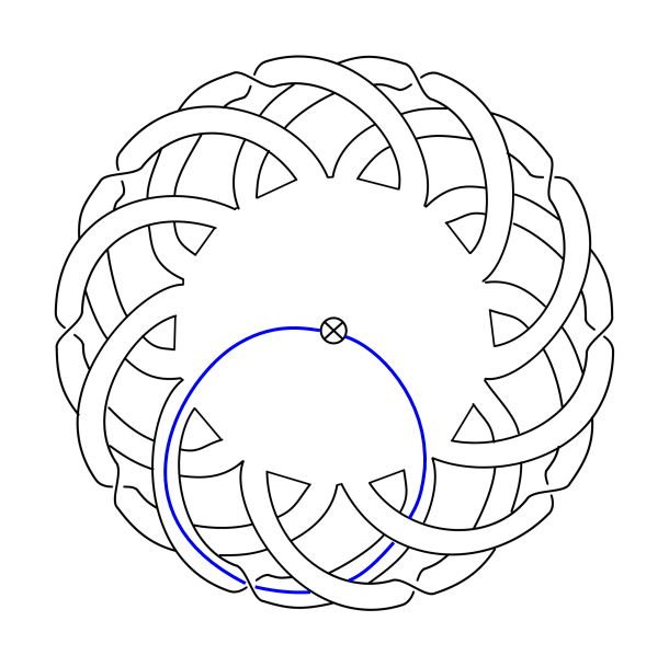
Figure 2. The surface $\Sigma_{10,5}$ and the curve $c_{10}$.

Lemma 2.1.

The Euler characteristic of $\Sigma_{n,k}$ is $-n$.

Proof.

The disk with a crosscap has zero Euler characteristic (it is homeomorphic to a Möbius strip), and each attached twisted strip has contribution $-1$. ∎

Lemma 2.2.

The number of boundary components of $\Sigma_{n,k}$ is $\gcd(n,k)$.

Proof.

We will show that the number of boundary components of $\Sigma_{n,k}$ is the same as the number of orbits of the dynamical system $x\mapsto x+n-k$ in the group $\mathbf{Z}/2n\mathbf{Z}$. The number of such orbits is $\gcd(n-k,2n)=\gcd(k,n)$, since $n-k$ is odd.

To prove our claim, we identify $\mathbf{Z}/2n\mathbf{Z}$ with the $2n$ intervals in the cyclic order. We claim that the right endpoint of the interval at position $i$ lies on the same boundary component as the right endpoint of the interval at position $i+n-k$. One can see this by induction. In the case $k=n-1$, the cyclic order of labels is $1,1,\ldots,n,n$, so the twisted strips identify the right endpoint of every interval with the right endpoint of the next interval. When $k=n-3$, the cyclic order is $1,n,2,1,\ldots,n,n-1$, in which case every third right endpoint is on the same boundary component, and so on. ∎

Proposition 2.3.

The surface $\Sigma_{n,k}$ is homeomorphic to the nonorientable surface of genus $n-\gcd(k,n)+2$ with $\gcd(k,n)$ boundary components.

Proof.

The Euler characteristic of the nonorientable surface of genus $g$ with $b$ boundary components is $2-g-b$. By Lemmas 2.1 and 2.2, we obtain the equation $2-g-\gcd(k,n)=-n$. Rearranging, we obtain $g=n-\gcd(k,n)+2$. ∎

2.3. The curves

We construct a two-sided curve $c_{i}$ for each label $i=1,\ldots,n$ as follows. Each curve consists of two parts. One part of each curve is the core of the strip corresponding to the label. The other part is an arc inside the disk that passes through the crosscap and connects the corresponding two intervals. The curve $c_{10}$ is shown on Figure 2.

Note that every pair of curves intersects either once or not at all. The curves $c_{i}$ and $c_{j}$ are disjoint if and only if the two $i$ labels and the two $j$ labels link in the cyclic order. In other words, if the two $i$ labels separate the two $j$ labels.

Lemma 2.4.

The intersection graph of the curves $c_{i}$ on $\Sigma_{n,k}$ is $G_{n,k}$.

Proof.

We proof the lemma by induction. If $k=n-1$, then $s=1$, so the cyclic order is $1,1,2,2,\ldots,n,n$. Since the no two labels link, all pairs of curves intersect and the intersection graph is the complete graph $G_{n,n-1}$.

Now suppose $k$ is decreased by 2. Then $s$ is decreased by 1, and we obtain the cyclic order $1,n,2,1,3,2,\ldots,n,n-1$. As a consequence, 1 becomes linked with 2 and $n$. Hence the intersection graph is indeed $G_{n,k}$.

It is easy to see that every time $k$ is decreased by two each label is linked with two more labels, hence the intersection graph is always $G_{n,k}$. ∎

Lemma 2.5.

The curves $c_{i}$ can be marked so that all intersections are inconsistent.

Proof.

Choose markings for the $c_{i}$ which are invariant under the rotational symmetry, see Figure 3. The marking of the curves is indicated by the coloring as follows. Consider the orientable surface obtained by removing the crosscap and cutting the strips attached to the disk in the middle. Choose an orientation of this surface. Then color the arcs composing the curves using red and blue depending on whether the orientation of the neighborhood of the curve matches the orientation of the surface or not. Note that the color of a curve changes when it goes through the crosscap or the middle of a strip.

Since blue and red meets at every intersection, the marking is inconsistent. ∎

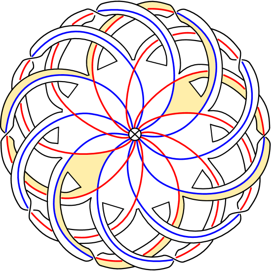
Figure 3. A collection of filling inconsistently marked curves.

2.4. The mapping classes

Denote by $r$ the rotation of $\Sigma_{n,k}$ by one click in the clockwise direction. Define the mapping class

$$f_{n,k}=r\circ T_{c_{1}}$$

where $T_{c_{1}}$ is a Dehn twist about the curve $c_{1}$. (There are two possible directions for the Dehn twist, but either choice works for our purposes.) Note that

$$f_{n,k}^{n}=T_{c_{n}}\circ\cdots\circ T_{c_{1}},$$

so $f_{n,k}^{n}$ arises from Penner’s construction. In particular, $f_{n,k}^{n}$ is pseudo-Anosov and so is $f_{n,k}$.

We remark that for $k=n-1$, the mapping class $f_{n,k}$ coincides with the nonorientable Arnoux-Yoccoz mapping class $h_{n-1}$, described as a product of a Dehn twist and a finite order mapping class by the authors in [LS18a].

Proposition 2.6.

The stretch factor of $f_{n,k}$ is the largest root of $x^{n}-x^{n-r}-x^{n-r-1}-\cdots-x^{r+1}-x^{r}-1$, where $r=\frac{n-k+1}{2}$.

Proof.

To compute the stretch factor, we use Penner’s approach in the section titled “An upper bound by example” in [Pen91]. Penner constructed an invariant bigon track by smoothing out the intersections of the curves $c_{i}$. Each $c_{i}$ defines a characteristic measure $\mu_{i}$ on this bigon track, defined by assigning 1 to the branches traversed by $c_{i}$ and zero to the rest. The cone generated by the $\mu_{i}$ is invariant under both $T_{c_{1}}$ and $r$, hence it contains the unstable foliation, and the stretch factor is given by the largest eigenvalue of the action of $r\circ T_{c_{1}}$ on this cone. The rotation $r$ acts by a permutation matrix and the matrix corresponding to $T_{c_{1}}$ is the sum of the identity matrix and matrix obtained by the intersection matrix $i(C,C)$ by zeroing out all rows except the first row. The product of these two matrices takes the following form:

$$\begin{pmatrix}0&1&0&0&0&0&0&0&0&0\\ 0&0&1&0&0&0&0&0&0&0\\ 0&0&0&1&0&0&0&0&0&0\\ 0&0&0&0&1&0&0&0&0&0\\ 0&0&0&0&0&1&0&0&0&0\\ 0&0&0&0&0&0&1&0&0&0\\ 0&0&0&0&0&0&0&1&0&0\\ 0&0&0&0&0&0&0&0&1&0\\ 0&0&0&0&0&0&0&0&0&1\\ 1&0&0&1&1&1&1&1&0&0\\ \end{pmatrix}$$

This particular matrix belongs to $f_{10,5}$.

This matrix is the companion matrix of the polynomial in the statement of the proposition. Hence the characteristic polynomial of this matrix is indeed that polynomial. ∎

Our next goal is to determine the singularity structure of the mapping classes $f_{n,k}$. For this, first we need a lemma.

Consider the complementary regions of the curves $\{c_{1},\ldots,c_{n}\}$. There are two types of regions depending on whether a region contains a boundary component of $\Sigma_{n,k}$ (type 1) or not (type 2). A region of type 1 is an annulus that is bounded by a boundary component $\beta$ of $\Sigma_{n,k}$ on one side and by a polygonal path consisting of arcs of the curves $c_{i}$ on the other side. The shaded region on Figure 3 illustrates a region of type 1.

Lemma 2.7.

The length of these polygonal paths is $\frac{4n}{\gcd(k,n)}$.

Proof.

This follows from the observation that every point in the orbit in $\mathbf{Z}/2n\mathbf{Z}$ corresponding to the boundary component $\beta$ (see the proof of Lemma 2.2) has two associated arcs. Since the number of orbits is $\gcd(k,n)$, the length of each orbit is $\frac{2n}{\gcd(k,n)}$, and hence the length of the polygonal path is twice this quantity. ∎

Proposition 2.8.

The pseudo-Anosov mapping class $f_{n,k}$ has $gcd(k,n)$ singularities, one for each boundary component. The number of prongs of each singularity is $\frac{2n}{\gcd(k,n)}$.

Proof.

Each complementary region of the curves $\{c_{1},\ldots,c_{n}\}$ contains either one singularity or none. The number of prongs of a singularity equals the number of cusps of the bigon track obtained by the smoothing process that are contained in the same region as the singularity. If the number of cusps is 2, then the region does not contain a singularity. If the number of cusps is $k>2$, then it contains a $k$-pronged singularity.

Regions of type 2 are rectangles (bounded by four subarcs of the curves $c_{i}$), and hence contain two cusps. So they do not correspond to singularities.

The lengths of the polygonal paths bounding regions of type 1 are $\frac{4n}{\gcd(k,n)}$ by Lemma 2.7, so the number of cusps in these regions is $\frac{2n}{\gcd(k,n)}$. Therefore the singularities have that many prongs. By Lemma 2.2, the number of such regions is $\gcd(k,n)$, so that is also the number of the singularities. ∎

As a corollary of Propositions 2.6, 2.8 and 2.3, we have the following.

Corollary 2.9.

There exist pseudo-Anosov mapping classes with an orientable invariant foliation on the surfaces $N_{g}$ with the data below. All of these examples belong to the family $f_{n,k}$ for the $n$ and $k$ shown in the table.

$g$	$n$	$k$	$\lambda(f_{n,k})$	minimal polynomial	singularity type
4*	3	2	1.83929	$x^{3}-x^{2}-x-1$	(6)
5*	6	3	1.51288	$x^{4}-x^{3}-x^{2}+x-1$	(4,4,4)
6*	5	2	1.42911	$x^{5}-x^{3}-x^{2}-1$	(10)
7*	10	5	1.42198	$x^{6}-x^{5}-x^{3}+x-1$	(4,4,4,4,4)
8*	7	2	1.28845	$x^{7}-x^{4}-x^{3}-1$	(14)
9	8	3	1.35680	$x^{8}-x^{5}-x^{4}-x^{3}-1$	(16)
10*	9	2	1.21728	$x^{9}-x^{5}-x^{4}-1$	(18)
11	12	3	1.22262	$\frac{x^{12}-x^{7}-x^{6}-x^{5}-1}{x^{2}+x+1}$	(8,8,8)
12*	11	2	1.17429	$x^{11}-x^{6}-x^{5}-1$	(22)
13	22	11	1.27635	$x^{12}-x^{11}-x^{6}+x-1$	(411)
14*	13	2	1.14551	$x^{13}-x^{7}-x^{6}-1$	(26)
15	14	3	1.18750	$x^{14}-x^{8}-x^{7}-x^{6}-1$	(28)
16*	15	2	1.12488	$x^{17}-x^{9}-x^{8}-1$	(30)
17	18	3	1.14259	$\frac{x^{18}-x^{10}-x^{9}-x^{8}-1}{x^{2}+x+1}$	(12,12,12)
18*	17	2	1.10938	$x^{19}-x^{10}-x^{9}-1$	(34)
19	18	5	1.20514	$x^{18}-x^{11}-x^{10}-x^{9}-x^{8}-x^{7}-1$	(36)
20*	19	2	1.09730	$x^{23}-x^{12}-x^{11}-1$	(38)

(4¹¹ means that there are 11 singularities with 4 prongs.)

In each genus, the family $f_{n,k}$ contains several examples. In the table above, we have listed only the example with the smallest stretch factor. In the starred cases, we will be able to certify that the given stretch factors are not only minimal in the family $f_{n,k}$ but among all pseudo-Anosov maps with an orientable invariant foliation.

3. Orientation-reversing pseudo-Anosov mapping classes on odd genus surfaces

In this section, we construct an orientation-reversing pseudo-Anosov mapping class with small stretch factor on every odd genus orientable surface. The construction is analogous to the construction in the previous section, but simpler. As in the previous section, we separate the construction of the surfaces, the curves and finally the mapping classes.

3.1. The surfaces

For every $k\geq 2$, consider the surface $\Sigma_{k}$ obtained by chaining together $2k$ annuli in a cycle as on Figure 4.

Figure 4. The surface $\Sigma_{k}$.

Proposition 3.1.

The number of boundary components of $\Sigma_{k}$ is 4 if $k$ is even and 2 if  $k$ is odd.

Proof.

The boundary of $\Sigma_{k}$ is composed of $8k$ arcs, 4 arcs for each annulus. Our goal is to determine which of them belong to the same boundary component.

Denote by $r$ the rotation of $\Sigma_{k}$ by one click. By tracing the boundary, one can see that every boundary point $x$ lies on the same boundary component as $r^{4}(x)$. Moreover, the path between $x$ and $r^{4}(x)$ traverses each of the 4 types of arcs exactly once. Therefore it suffices to pick any boundary point $x$ and determine into how many equivalence classes the set $\{x,r(x),\ldots,r^{2k-1}(x)\}$ falls apart. The number of such equivalence classes is 4 if $k$ is even and 2 if $k$ is odd. ∎

Proposition 3.2.

The surface $\Sigma_{k}$ is homeomorphic to $S_{k-1,4}$ if $k$ is even and $S_{k,2}$ if $k$ is odd.

Proof.

We have $\chi(\Sigma_{k})=2k$. From the equation $\chi=2-2g-b$, where $g$ is the genus and $b$ is the number of boundary components, it follows that $g=k+1-\frac{b}{2}$. The statement now follows from Proposition 3.1. ∎

As a consequence, the construction only produces odd genus examples.

3.2. The curves

From now on, suppose that $k$ is even. Consider the set $C=\{c_{1},\ldots,c_{2k}\}$ of core curves of the $2k$ annuli. Our numbering will differ from the standard cyclic numbering; we will explain this shortly. As in Section 2.3, any rotationally symmetric marking of the curves is an inconsistent marking.

The intersection graph of $C$ is a cycle of length $2k$. We draw this cycle as on Figure 5: the vertices are the vertices of a regular polygon and every vertex is connected to the two vertices that are the second furthest in the cyclic order. We number the curves according to the cyclic orientation induced by this picture.

Figure 5. Our unusual way of numbering the curves. For example, the curve $c_{1}$ intersects $c_{k}$ and $c_{k+2}$, not $c_{2}$ and $c_{2k}$.

3.3. The mapping classes

Denote by $r$ the rotation of $\Sigma_{k}$ (see Figure 4) by one click in the clockwise direction. Since $c_{i}$ and $r(c_{i})$ intersect for all $i$, the rotation $r$ induces a rotation of the cycle on Figure 5 by $k-1$ clicks. So $r^{k-1}$ rotates the cycle by $(k-1)^{2}=k^{2}-2k+1$ clicks, which is congruent to 1 modulo $2k$ if $k$ is even. Therefore $r^{k-1}$ induces rotating the cycle on Figure 5 by one click (in the clockwise direction, assuming that we have chosen the numbering of the curves accordingly). In particular, we have $r^{k-1}(c_{i+1})=c_{i}$.

We are now ready to define the mapping class:

$$\psi_{k}=r^{k-1}\circ T_{c_{1}}.$$

Note that

$$\psi_{k}^{2k}=T_{c_{2k}}\circ\cdots\circ T_{c_{1}},$$

so $\psi_{k}^{2k}$ arises from Penner’s construction. In particular, $\psi_{k}^{2k}$ is pseudo-Anosov and so is $\psi_{k}$. Note that while $\psi_{k}^{2k}$ is orientation-preserving, $\psi_{k}$ is orientation-reversing. This follows from the observation that $T_{c_{1}}$ is orientation-preserving and $r$ is orientation-reversing.

Proposition 3.3.

The stretch factor of $\psi_{k}$ is the largest root of $x^{2k}-x^{k+1}-x^{k-1}-1$.

Proof.

The proof is similar to the proof of Proposition 2.6. We have

$$i(C,C)=\begin{pmatrix}0&0&0&1&0&1&0&0\\ 0&0&0&0&1&0&1&0\\ 0&0&0&0&0&1&0&1\\ 1&0&0&0&0&0&1&0\\ 0&1&0&0&0&0&0&1\\ 1&0&1&0&0&0&0&0\\ 0&1&0&1&0&0&0&0\\ 0&0&1&0&1&0&0&0\end{pmatrix}\quad\mbox{and}\quad M=\begin{pmatrix}0&1&0&0&0&0&0&0\\ 0&0&1&0&0&0&0&0\\ 0&0&0&1&0&0&0&0\\ 0&0&0&0&1&0&0&0\\ 0&0&0&0&0&1&0&0\\ 0&0&0&0&0&0&1&0\\ 0&0&0&0&0&0&0&1\\ 1&0&0&1&0&1&0&0\end{pmatrix}$$

where $M$ is the matrix of the action of $\psi_{k}$ on the cone of measures (the product of a permutation matrix and the sum of the identity matrix and the first row of $i(C,C)$). The matrices above illustrate the case $k=4$. The matrix $M$ is the companion matrix of the polynomial in the proposition. ∎

Proposition 3.4.

The pseudo-Anosov mapping class $\psi_{k}$ has four $k$-pronged singularities.

Proof.

By Proposition 3.1 and its proof, each of the four boundary components of $\Sigma_{k}$ consists of $2k$ arcs if $k$ is even. There is a prong for every second corner of the boundary path, therefore there are $k$ prongs for each singularity. ∎

Corollary 3.5.

There exist orientation-reversing pseudo-Anosov mapping classes with orientable invariant foliations on the surfaces $S_{g}$ with the data below. All of these examples belong to the family $\psi_{k}$ for the $k$ shown in the table.

$g$	$k$	$\lambda(\psi_{k})$	largest root of	singularity type
1	2	1.61803	$x^{2}-x-1=\frac{x^{4}-x^{3}-x-1}{x^{2}+1}$	no singularities
3	4	1.25207	$x^{8}-x^{5}-x^{3}-1$	(4,4,4,4)
5	6	1.15973	$x^{12}-x^{7}-x^{5}-1$	(6,6,6,6)
7	8	1.11707	$x^{16}-x^{9}-x^{7}-1$	(8,8,8,8)
9	10	1.09244	$x^{20}-x^{11}-x^{9}-1$	(10,10,10,10)
11	12	1.07638	$x^{24}-x^{13}-x^{11}-1$	(12,12,12,12)

Proof.

The statement follows from Propositions 3.3, 3.4 and 3.2. The reason we have no singularities in the genus 1 case is that by Proposition 3.4 the “singularities” have two prongs, so they are not actually singularities. ∎

We remark that in the genus 1, there is an alternative, simpler construction that yields the same stretch factor. Consider the matrix

$$M=\begin{pmatrix}0&1\\ 1&1\\ \end{pmatrix}$$

with determinant $-1$. The corresponding linear map $\mathbf{R}^{2}\to\mathbf{R}^{2}$ maps $\mathbf{Z}^{2}$ to $\mathbf{Z}^{2}$, hence it descends to an Anosov diffeomorphism $f$ of the torus $\mathbf{R}^{2}/\mathbf{Z}^{2}$. Its stretch factor is the largest root of the $x^{2}-x-1$, the characteristic polynomial of $M$.

4. Restrictions on polynomials

Pseudo-Anosov stretch factors are roots of integral polynomials. The properties of these integral polynomials are similar, but slightly different depending on whether a pseudo-Anosov mapping class is an orientation-preserving or orientation-reversing mapping class on an orientable surface or a mapping class on a nonorientable surface. In this section, we discuss these properties for nonorientable surfaces and orientation-reversing mapping classes.

A polynomial $p(x)$ of degree $n$ is called reciprocal if $p(x)=\pm x^{n}p(x^{-1})$, in other words, when its coefficients are the same in reverse order up to sign. Analogously, we define $p(x)$ to be skew-reciprocal if $p(x)=\pm x^{n}p(-x^{-1})$.

Proposition 4.1.

Let $\psi:N_{g}\to N_{g}$ be a pseudo-Anosov map with a transversely orientable invariant foliation on the closed non-orientable surface $N_{g}$ of genus $g$. Then its stretch factor $\lambda$ is a root of a (not necessarily irreducible) polynomial $p(x)\in\mathbf{Z}[x]$ with the following properties:

1. $\deg(p)=g-1$.

2. $p(x)$ is monic and its constant coefficient is $\pm 1$.

3. The absolute values of the roots of $p(x)$ other than $\lambda$ lie in the open interval $(\lambda^{-1},\lambda)$. In particular, $p(x)$ is not reciprocal or skew-reciprocal.

4. $p(x)$ is reciprocal mod 2.

Proof.

Note that exactly one of the stable and unstable foliations is transversely orientable (otherwise the surface itself would be orientable). We will assume that it is the stable foliation, otherwise we replace $\psi$ by its inverse.

Consider the action $\psi^{*}:H^{1}(N_{g};\mathbf{R})\to H^{1}(N_{g};\mathbf{R})$ defined by pullback on cohomology with real coefficients. Since the stable foliation is transversely orientable, it is represented by a closed real 1-form, that is, an element of $H^{1}(N_{g};\mathbf{R})$. The stable foliation $\mathcal{F}^{s}$ is the one whose leaves are contracting and hence the surface is expanding in the transverse direction. Therefore the measure of a transverse arc in the pullback $\psi^{*}(\mathcal{F}^{s})$ is $\lambda$ times its measure in $\mathcal{F}^{s}$. Hence $\mathcal{F}^{s}$ is an eigenvector of the map $\psi^{*}$ with eigenvalue $\lambda$ or $-\lambda$.

Let $p(x)$ be the characteristic polynomial of $\psi^{*}$. Note that $\dim(H^{1}(N_{g},\mathbf{R}))=g-1$, hence $\deg(p)=g-1$. This proves (1).

The polynomial $p(x)$ has integral coefficients, since $\psi^{*}$ restricts to an action $H^{1}(N_{g};\mathbf{Z})\to H^{1}(N_{g};\mathbf{Z})$. This restriction is invertible, since the action of $\operatorname{Mod}(N_{g})$ on $H^{1}(N_{g};\mathbf{Z})$ is a group representation, so the determinant of $\psi^{*}$ is $\pm 1$. Therefore the constant coefficient of $p(x)$ is $\pm 1$. Also, as a characteristic polynomial, $p(x)$ is monic. This proves (2).

It is a standard fact from the theory of orientation-preserving pseudo-Anosov mapping classes on orientable surfaces that stretch factors are strictly maximal among their Galois conjugates. Moreover, in case the invariant foliations are orientable, the spectral radius of the action induced on the first homology equals the stretch factor, and every other eigenvalue is strictly smaller, see, for example, [McM03, Theorem 5.3 (1)]. Applying this result to the orientation-preserving lift $\tilde{\psi}:S_{g-1}\to S_{g-1}$ of $\psi$ to the orientable double cover $S_{g-1}$ of $N_{g}$, we obtain that any root $\lambda^{\prime}$ of $p(x)$ other than $\pm\lambda$ satisfies $|\lambda^{\prime}|<|\lambda|$. Applying the same theorem for $\tilde{\psi}^{-1}$, we conclude that any root $\lambda^{\prime}$ of $p(x)$ other than $\pm\lambda^{-1}$ satisfies $|\lambda^{\prime-1}|<|\lambda|$. Therefore absolute values of the roots of $p(x)$ other than $\pm\lambda$ and possibly $\pm\lambda^{-1}$ lie in the open interval $(\lambda^{-1},\lambda)$. However, it was shown in the proof of [Str18, Proposition 2.3] that if $\lambda$ or $-\lambda$ is a root of $p(x)$, then $\lambda^{-1}$ and $-\lambda^{-1}$ cannot be roots of $p(x)$, hence mentioning the edge case $\pm\lambda^{-1}$ in the previous sentence is not necessary.

If $p(x)$ was reciprocal, then $\lambda$ and $\lambda^{-1}$ or $-\lambda$ and $-\lambda^{-1}$ would have to be roots. If it was skew-reciprocal, then $\lambda$ and $-\lambda^{-1}$ or $-\lambda$ and $\lambda^{-1}$ would have to be roots. As we have just shown, these scenarios are impossible, because $\pm\lambda^{-1}$ is not a root of $p(x)$. This proves (3).

The fact that $p(x)$ is reciprocal mod 2 was shown in [Str18, Proposition 4.2]. This justifies (4).

Finally, notice that we have not guaranteed that $\lambda$ is a root of $p(x)$—we have only shown that either $\lambda$ or $-\lambda$ is a root. If it is $-\lambda$, then the polynomial $p(-x)$ or $-p(-x)$ satisfies all the required properties. ∎

We call a $2n\times 2n$ matrix $A$ anti-symplectic if it the corresponding linear transformation sends the standard symplectic form on $\mathbf{R}^{2n}$ to its negative. Formally, this can be written as

$$AJA^{T}=-J$$

where $J=\begin{pmatrix}0&I\\ -I&0\\ \end{pmatrix}$ and $I$ is the $n\times n$ identity matrix.

Proposition 4.2.

The characteristic polynomial $p(x)$ of a $2n\times 2n$ anti-symplectic matrix is skew-reciprocal.

Proof.

Let $A$ be an $2n\times 2n$ anti-symplectic matrix. Since $A^{2}$ is symplectic, we have $\det(A^{2})=1$ and $\det(A)=\pm 1$. Since $\det(J)=1$, we have

$$p(x) =\det(A-xI)=\det(AJ-xJ)=\det(AJ+xAJA^{T})$$

$$=\det(A)\det(J)\det(I+xA^{T})=\pm\det(I+xA)$$

$$=\pm x^{2n}\det\left(A+x^{-1}I\right)=\pm x^{2n}p(-x^{-1}),$$

hence $p(x)$ is skew-reciprocal. ∎

The proof above is a straightforward modification of the standard proof of the fact that the characteristic polynomials of symplectic matrices are reciprocal.

Proposition 4.3.

Let $\psi:S_{g}\to S_{g}$ be an orientation-reversing pseudo-Anosov map with transversely orientable invariant foliations. Then its stretch factor $\lambda$ is a root of a (not necessarily irreducible) polynomial $p(x)\in\mathbf{Z}[x]$ with the following properties:

1. $\deg(p)=2g$.

2. $p(x)$ is monic and its constant coefficient is $(-1)^{g}$.

3. $p(x)=(-1)^{g}x^{2g}p(-x^{-1})$.

4. $p(-\lambda^{-1})=0$.

5. The absolute values of the roots of $p(x)$ other than $\lambda$ and $-\lambda^{-1}$ lie in the open interval $(\lambda^{-1},\lambda)$.

Proof.

Let $p(x)$ be the characteristic polynomial of $\psi_{*}:H_{1}(S_{g})\to H_{1}(S_{g})$. Clearly, (1) holds. Similarly to the proof of Proposition 4.1, we obtain (5) by a reduction to the known statement for orientation-preserving pseudo-Anosov mapping classes. This time, we directly obtain (5) by applying [McM03, Theorem 5.3] to the square of $\psi$.

An orientation-reversing homeomorphism sends the intersection form on $H_{1}(S_{g})$ to its negative. Proposition 4.2 implies that $p(x)=\pm x^{2g}p(-x^{-1})$. To decide which sign is right, we only need to compute the sign of the constant coefficient of $p(x)$. If the constant coefficient $1$, then the sign is positive. If the constant coefficient is $-1$, then the sign is negative. To put this in another way, we have

(4.1) $$p(x)=p(0)x^{2g}p(-x^{-1}).$$

For orientation-preserving homeomorphisms, the action on homology is symplectic, hence its determinant is $+1$. It follows that, for fixed $g$, the determinant is either $+1$ for all orientation-reversing homeomorphisms of $S_{g}$ or $-1$ for all orientation-reversing homeomorphisms of $S_{g}$. It is sufficient to check only one homeomorphism to decide which one. For example, consider the reflection $i:S_{g}\to S_{g}$ about the plane containing the curves $b_{i}$ on Figure 6.

2pt $a_{1}$ [ ] at 14 37 $a_{2}$ [ ] at 77 37 $b_{1}$ [ ] at 47 45 $b_{2}$ [ ] at 111 44

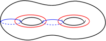
Figure 6. The standard homology basis for $S_{2}$.

The curves $\{a_{1},\ldots,a_{g},b_{1},\ldots,b_{g}\}$ form a homology basis. We have $i(b_{i})=b_{i}$ and $i(a_{i})=-a_{i}$ for all $i$. So the matrix of $A$ is a diagonal matrix whose diagonal contains $1$s and $-1$s, $g$ of each. Hence the determinant is $(-1)^{g}$ and we have shown (2).

Item (3) follows from equation (4.1) and the fact $p(0)=(-1)^{g}$ we have just shown.

Either $\lambda$ or $-\lambda$ is a root of $p(x)$. If it is $-\lambda$, we may replace $p(x)$ with $p(-x)$; the previously proven properties remain true. Finally, (4) follows from (3) by setting $x=\lambda$. ∎

We are now ready to prove Theorem 1.10. We emphasize that, unlike in the previous propositions, in this theorem we are not assuming that the surface is closed or that the pseudo-Anosov mapping class has a transversely orientable invariant foliation.

Proof of Theorem 1.10.

An irreducible polynomial $p(x)\in\mathbf{Z}[x]$ with a (complex) root $\alpha$ on the unit circle is reciprocal. This is because then $\alpha^{-1}$ is also a root of $p(x)$, therefore $\alpha$ is a root of the polynomial $x^{d}p(x^{-1})$, where $d$ is the degree of $p(x)$. But the minimal polynomial is unique up constant factor, so $x^{d}p(x^{-1})=\pm p(x)$. Hence $p(x)$ is indeed reciprocal. So if a stretch factor $\lambda$ has a Galois conjugate on the unit circle, then the minimal polynomial of $\lambda$ is reciprocal and $\lambda^{-1}$ is also a root of the minimal polynomial.

However, by [Str18, Proposition 2.3], $\lambda$ and $\lambda^{-1}$ are not Galois conjugates if $\lambda$ is a stretch factor of a pseudo-Anosov map (possibly with no orientable invariant foliations) on a nonorientable surface (possibly with punctures). This completes the proof in the case when the pseudo-Anosov map is supported on a nonorientable surface.

We now prove the orientation-reversing case. If our surface is closed, then, by Proposition 4.3, $\lambda$ and $\lambda^{-1}$ are not Galois conjugates if $\lambda$ is a stretch factor of an orientation-reversing pseudo-Anosov map with orientable invariant foliations. If the foliations are not orientable, we can lift the map to the orientation double cover of the foliations to obtain an orientation-reversing pseudo-Anosov map with orientable invariant foliations and with the same stretch factor. Therefore $\lambda$ and $\lambda^{-1}$ are not Galois conjugates in this case, either.

If our surface has punctures, then we can fill in the punctures after making the foliations orientable to obtain a pseudo-Anosov map with the same stretch factor on a closed surface, reducing to the closed case discussed in the previous paragraph. This completes the proof in the case when the pseudo-Anosov map is orientation-reversing. ∎

5. Elimination of polynomials

In this section we first prove bounds on the sum of $k$th powers of roots of a polynomial when the absolute values of the roots are bounded by some $r>1$. These bounds are improved versions of Lemma A.1. of [LT11b], using the special properties of the polynomials in Propositions 4.1 and 4.3.

Then we describe how we use this lemma and Propositions 4.1 and 4.3 in order to systematically narrow down the set of possible minimal polynomials of the minimal stretch factors.

5.1. Power sum bounds

We begin by proving two elementary lemmas.

Lemma 5.1.

Suppose $r>1$ and $r^{-1}\leq a_{1},\ldots,a_{d}\leq r$ are positive real numbers such that $a_{1}\cdots a_{d}=1$. Then

$$\sum_{i=1}^{d}a_{i}\leq\begin{cases}n(r+r^{-1})&\mbox{if $d=2n$ is even}\\ n(r+r^{-1})+1&\mbox{if $d=2n+1$ is odd.}\end{cases}$$

Proof.

The function $x\mapsto x+x^{-1}$ is increasing on the interval $x\geq 1$. So if there are $i\neq j$ so that $r^{-1}<a_{i},a_{j}<r$, then we can increase the sum by moving $a_{i}$ and $a_{j}$ away from each other by keeping their product unchanged, until at least one of them is $r^{-1}$ or $r$. After every such operation, the number of $a_{i}$ that are equal to $r^{-1}$ or $r$ increases. So eventually we get to a point where at most one $a_{i}$ is not $r^{-1}$ or $r$. When $d=2n$, no such $a_{i}$ can exist, and exactly half of the $a_{i}$ equal $r$, the other half $r^{-1}$, otherwise their product would not be 1. When $d=2n+1$, exactly one such$a_{i}$ exists, it equals 1 and exactly half of the remaining $a_{i}$ equal $r$, the other half $r^{-1}$. ∎

Lemma 5.2.

Suppose $r>1$ and $a_{1},\ldots,a_{d}$ are positive real numbers such that $r^{-1}\leq a_{1}\leq\ldots\leq a_{d}\leq r$ and $a_{1}\cdots a_{d}=1$ and $a_{1}\geq a_{d}^{-1}$. Then

$$a_{d}-\sum_{i=1}^{d-1}a_{i}\geq\begin{cases}\min\{2-2n,-(n-2)r-nr^{-1}\}&\mbox{if $d=2n$ is odd.}\\ \min\{1-2n,-(n-2)r-1-nr^{-1}\}&\mbox{if $d=2n+1$ is odd.}\end{cases}$$

Moreover, the inequalities are strict if $a_{1}>a_{d}^{-1}$.

Proof.

Similarly to the proof of Lemma 5.1, our approach is to change the numbers $a_{1},\ldots,a_{d-1}$ to increase $\sum_{i=1}^{d-1}a_{i}$ as much as possible while keeping the hypotheses true. Whenever there are $i\neq j$ such that $a_{d}^{-1}<a_{i},a_{j},<a_{d}$, we push $a_{i}$ and $a_{j}$ apart until at least one of them equals $a_{d}^{-1}$ or $a_{d}$. The end result is the same as before, so we have

$$a_{d}-\sum_{i=1}^{d-1}a_{i}\geq a_{d}-((n-1)a_{d}+na_{d}^{-1})=-(n-2)a_{d}-na_{d}^{-1}.$$

when $d=2n$ and

$$a_{d}-\sum_{i=1}^{d-1}a_{i}\geq a_{d}-((n-1)a_{d}+1+na_{d}^{-1})=-(n-2)a_{d}-1-na_{d}^{-1}$$

when $d=2n+1$. Since the function $x\mapsto-(n-2)x-nx^{-1}$ is concave, its minimum on the interval $[1,r]$ is taken at one of the endpoints.

The inequalities in the case $a_{1}>a_{d}^{-1}$ are strict, since in the optimal distribution there has to be an $a_{i}$ that takes the value $a_{d}^{-1}$. ∎

Now we apply Lemmas 5.1 and 5.2 for roots of polynomials.

Corollary 5.3.

Suppose $P(x)$ is a monic polynomial of degree $d$ with constant coefficient $\pm 1$. Let $z_{1},\ldots,z_{d}$ be the roots of $P(x)$ and let

$$p_{k}=z_{1}^{k}+\cdots+z_{d}^{k}$$

the $k$th power sum of the roots.

Suppose there is a root $\lambda>1$ such that all the other roots have absolute values in the interval $[\lambda^{-1},\lambda]$. For any $r>\lambda$, we have

$$\min\{2-2n,-(n-2)r^{k}-nr^{-k}\}\leq p_{k}\leq n(r^{k}+r^{-k})$$

if $d=2n$ is even and

$$\min\{1-2n,-(n-2)r^{k}-1-nr^{-k}\}\leq p_{k}\leq n(r^{k}+r^{-k})+1$$

if $d=2n+1$ is odd.

Moreover, strict inequality holds in the lower bound when no eigenvalue equals $\lambda^{-1}$.

Proof.

Let $z_{1},\ldots,z_{d}$ be the roots of $P(x)$ and let $a_{i}=|z_{i}|^{k}$ for every $i$. Note that $a_{1}\cdots a_{d}=1$ and $r^{-k}\leq a_{1},\ldots,a_{d}\leq r^{k}$. Assuming $a_{1}\leq\cdots\leq a_{d}$, we have $a_{d}=\lambda^{k}$. Since

$$a_{d}-\sum_{i=1}^{d-1}a_{i}\leq p_{k}=z_{1}^{k}+\cdots+z_{d-1}^{k}+\lambda^{k}\leq\sum_{i=1}^{d}a_{i},$$

the bounds follow from Lemma 5.1 and Lemma 5.2 ∎

5.2. Newton’s formulas

In this section, we recall Newton’s formulas that relate power sums of the roots to the coefficients of the polynomial.

We will use the notation

$$P(x)=x^{d}-c_{1}x^{d-1}-\cdots-c_{d-1}x\pm 1$$

for the coefficients of monic polynomials of degree $d$. As in the statement of 5.3, we denote by $p_{k}$ the $k$th power sum of the roots of $P(x)$.

Newton’s formulas relating power sums and symmetric polynomials can be stated either as

(5.1) $$p_{k}=-c_{1}p_{k-1}-c_{2}p_{k-2}-\cdots-c_{k-1}p_{1}-kc_{k}$$

or as

(5.2) $$c_{k}=\frac{-c_{1}p_{k-1}-c_{2}p_{k-2}-\cdots-c_{k-1}p_{1}-p_{k}}{k}$$

for all $1\leq k\leq d-1$.

As Lanneau and Thiffeault point out in Section A.1 of [LT11b], is it more computationally efficient to bound the power sums $p_{i}$ and using Newton’s formulas to compute the coefficients $c_{k}$ from the $p_{i}$ than to bound the coefficients directly. This is because many scenarios get ruled out just because the numerator in equation (5.2) is not divisible by $k$.

5.3. The polynomial elimination algorithm

We give a lower bound on the minimal stretch factor $\delta^{+}(N_{g})$ by a systematic elimination of polynomials. We describe this process below. In order to illustrate the effect of each step in the algorithm, we give the number of candidate polynomials left after each step when $g=12$ (when the degree is 11).

Algorithm 5.4.

Let $d\geq 4$, $g=d-1$ and $r>1$ such that $\delta^{+}(N_{g})<r$. Perform the following steps in order to obtain a small set of polynomials of degree $g$ that include one polynomial whose root is $\delta^{+}(N_{g})$:

1. Compute the possible values of $p_{1},\ldots,p_{d-1}$ using the bounds given by 5.3. For $d=11$, the total number of combinations is $20\cdot 20\cdot 21\cdot 23\cdot 24\cdot 27\cdot 30\cdot 34\cdot 38\cdot 43=10,641,541,131,648,000$.

2. Compute the coefficients $c_{1},\ldots,c_{d-1}$ using Equation 5.2, keeping only the cases when all $c_{i}$ are integers. 57,643,952 cases remain.

3. Discard all cases where the polynomial is not reciprocal mod 2. 1,808,922 cases remain.

4. Try $\pm 1$ for the constant coefficient. We now doubled the number of cases to 3,617,844.

5. Consider the reciprocal polynomial $P^{*}(x)=\pm x^{d}P(x^{-1})$ (with the sign chosen so that the polynomial is monic), and use Equation 5.1 to compute the power sums  $p^{*}_{1},\ldots,p^{*}_{d-1}$ of this polynomial from the reversed sequence  $\pm c_{d-1},\ldots,\pm c_{1}$ of coefficients, where the signs here depend on the sign chosen in the previous step. Discard the cases that do not satisfy the bounds of 5.3. 5075 cases remain.

6. Test the remaining polynomials by Newton’s method for finding roots. Start with the upper bound for the Perron root. Since the polynomial is increasing and convex in $[\lambda,\infty)$, we should get a decreasing sequence of $x$-values larger than $\lambda$. Discard the cases when this fails. Stop when two consecutive $x$-values are very close to each other. 421 cases remain.

7. Discard the polynomials where the largest eigenvalue in absolute value is not real. 86 cases remain.

8. Discard the cases where the multiplicity of the largest eigenvalue is larger than 1. 54 cases remain.

9. Discard the cases when there is a root with absolute value less than or equal to $\lambda^{-1}$. 33 cases remain.

10. Discard the cases where the largest eigenvalue is larger than our upper bound. 1 case remains.

In practice, the first three steps are implemented in a more sophisticated way. Our computers cannot handle as many as $10,641,541,131,648,000$ cases, so the implementation does not actually consider all those combinations. It first chooses a value for $p_{1}$ and sets $c_{1}=-p_{1}$ by (5.2). Then it has to choose a value for $p_{2}$ of the same parity as $p_{1}$, since $c_{2}=-\frac{c_{1}p_{1}-p_{2}}{2}$. Similarly, the value chosen for $p_{3}$ is then determined mod 3, therefore a huge number of combinations for the $p_{i}$ are never considered. Also, once more than half of the $c_{i}$ are computed, we obtain additional constraints on the $p_{i}$, since our polynomial has to be reciprocal mod 2. Since these divisibility checks are done early, and not after the whole polynomial is constructed, a huge number of cases gets eliminated early.

The idea of bounding the coefficients using power sums as in steps (1) and (2) instead of using symmetric polynomials to express the coefficients in terms of the roots is due to Lanneau and Thiffeault [LT11b]. As the numbers suggest, these are the steps that are responsible for bringing the size of the set of possible polynomials down from an astronomical size to one that is approachable by computers.

Step (3) is special to nonorientable surfaces and is also crucial. Without this step, not only would the searching process be much slower, but there are quite a few polynomials that pass all the other tests but this is the only step that eliminates them. Perhaps this step is the main reason for why we do not need Lefschetz number tests unlike Lanneau and Thiffeault in the orientable case.

Step (5) is also special to nonorientable surfaces, since in the orientable case the polynomials are reciprocal, so the reciprocal polynomial does not contain any additional information. This was one of the last tests we added, and this reduced the running time of the algorithm for the $d=11$ case from several hours to a few minutes. The reason this works so effectively is that in most of the coefficient sequences at this point, the last few coefficients ($c_{d-1}$, $c_{d-2}$, etc.) are much bigger than the required bounds.

Step (6) is another computationally inexpensive test that quickly eliminates a large fraction of the polynomials. The idea of this test is also due to Lanneau and Thiffeault.

The most computationally expensive part is computing the roots. We only compute the roots after Step (6), only in 421 cases. So in terms of total time, actually steps (1)–(6) take more than 99% of the running time.

We use a very similar algorithm in order to give a lower bound for the minimal stretch factor $\delta^{+}_{rev}(S_{g})$ among orientation-reversing pseudo-Anosov maps. The difference is that we use the properties from Proposition 4.3 instead of the ones from Proposition 4.1. Our implementation of these algorithms can be found at https://github.com/b5strbal/polynomial-filtering.

5.4. Minimal stretch factors

We are now ready to single out the minimal stretch factor $\delta^{+}(N_{g})$ among pseudo-Anosov homeomorphisms with an orientable invariant foliation for certain nonorientable closed surfaces $N_{g}$. Theorem 1.1 is a direct consequence of 2.9 and Proposition 5.5 below.

Proposition 5.5.

Let $g$ and $r$ be as in one of the rows in the table below. Let $f$ be a pseudo-Anosov mapping class with an orientable invariant foliation on $N_{g}$ whose stretch factor $\lambda$ is smaller than $r$. Then $\lambda$ must be a root of the polynomial shown in the table.

In the cases where no polynomial is given, we have indicated to how many polynomials we were able to restrict the list of candidate polynomials.

$g$	$r$	Polynomial candidates	largest root
4	1.84	$x^{3}-x^{2}-x-1$	1.83929
5	1.52	$x^{4}-x^{3}-x^{2}+x-1$	1.51288
6	1.43	$x^{5}-x^{3}-x^{2}-1$	1.42911
7	1.422	$x^{6}-x^{5}-x^{3}+x-1$	1.42198
8	1.2885	$x^{7}-x^{4}-x^{3}-1$	1.28845
9	1.3568	18 candidates
10	1.2173	$x^{9}-x^{5}-x^{4}-1$	1.21728
11	1.22262	5 candidates
12	1.1743	$x^{11}-x^{6}-x^{5}-1$	1.17429
13	1.2764	288 candidates
14	1.14552	$x^{13}-x^{7}-x^{6}-1$	1.14551
15	1.1875	84 candidates
16	1.1249	$x^{15}-x^{8}-x^{7}-1$	1.12488
17	1.1426	16 candidates
18	1.10939	$x^{17}-x^{9}-x^{8}-1$	1.10938
20	1.09731	$x^{19}-x^{10}-x^{9}-1$	1.09730

Proof.

The proof consists of running Algorithm 5.4 and is computer-assisted. However, we will prove the proposition by hand in genus 4. We follow the first four steps explicitly, then (since only a handful of polynomials remain) we finish the proof with an ad hoc but simple argument.

Step (1): we have

$$-1=\min\{-1,1.84-1-1/1.84\}<p_{1}<1.84+1+1/1.84\approx 3.38,$$

therefore the possible values for $p_{1}$ are 0, 1, 2 and 3. We have

$$-1=\min\{-1,1.84^{2}-1-1/1.84^{2}\}<p_{2}<1.84^{2}+1+1/1.84^{2}\approx 4.68,$$

so the possible values for $p_{2}$ are 0, 1, 2, 3 and 4.

Step (2): By (5.2), we have $c_{1}=-p_{1}$ and $c_{2}=\frac{p_{1}^{2}-p_{2}}{2}$, therefore $p_{1}$ and $p_{2}$ have the same parity. Hence the possible pairs are $(0,0)$, $(0,2)$, $(0,4)$, $(1,1)$, $(1,3)$, $(2,0)$, $(2,2)$, $(2,4)$, $(3,1)$ and $(3,3)$.

Step (3): The pair $(p_{1},\frac{p_{1}^{2}-p_{2}}{2})$ also has the same parity, since our polynomial is reciprocal mod 2. That leaves the choices $(0,0)$, $(0,4)$, $(1,3)$, $(2,0)$, $(2,4)$, $(3,3)$ for $(p_{1},p_{2})$.

Step (4): We construct the list of possible polynomials.

1. $x^{3}\pm 1$

2. $x^{3}-2x\pm 1$

3. $x^{3}-x^{2}-x\pm 1$

4. $x^{3}-2x^{2}+2x\pm 1$

5. $x^{3}-2x^{2}\pm 1$

6. $x^{3}-3x^{2}+3x\pm 1$

The polynomial has to be irreducible, since the degree of a stretch factor on a nonorientable surface is at least three [Str17, Proposition 8.7.]. The polynomials where neither 1 nor $-1$ are roots are $x^{3}-x^{2}-x-1$, $x^{3}-2x^{2}+2x+1$, $x^{3}-2x^{2}-1$ and $x^{3}-3x^{2}+3x+1$. The second and fourth polynomial do not have a positive real root, and the third polynomial has a root that is approximately 2.2. That leaves us with $x^{3}-x^{2}-x-1$. ∎

We have stopped at genus 20 because of computational difficulties. The genus 18 case took about half a day to run on a single computer. In the genus 20 case the algorithm took about a day to complete when run parallel on 30 computers. We estimate that the genus 22 case would need to run for a few months on the same cluster of computers.

In the odd genus cases, the issue is not the running time, but the fact that our tests are not good enough to eliminate all polynomials that should be eliminated. In the hope of dealing with more odd genus cases, we have also implemented the Lefschetz number tests used by Lanneau and Thiffeault [LT11b, Section 2.3]. These tests help eliminate a large percentage of the remaining polynomials, but, unfortunately, not all. Table 2 below shows the polynomials that we could not eliminate in the genus 9, 11 and 13 cases, in addition to the polynomials that we have constructed in 2.9.

$g$	Polynomial	Stratum	Stretch factor
9	$(x^{7}-x^{4}-x^{3}-1)(x-1)$	$(4^{7})$	1.28845
	$(x^{7}-x^{5}-x^{2}-1)(x-1)$	$(4^{7})$	1.30740
11	$(x^{9}-x^{5}-x^{4}-1)(x-1)$	$(4^{9})$	1.21728
13	18 polynomials

Table 2. The polynomials and possible strata in genus 9, 11 that we cannot rule out using Algorithm 5.4 and Lefschetz arguments. The notation $a^{b}$ means an orbit of length $b$ consisting of $a$-pronged singularities.

Most of the polynomials that we are not able to eliminate are products of polynomials that appear in some lower genus and cyclotomic polynomials. We think that these polynomials should be possible to eliminate, but we do not know how. In particular, we think that in the genus 9 and 11 cases all three remaining polynomials could be eliminated, and we conjecture that the examples constructed in 2.9 are the minimal stretch factor examples (cf. Conjecture 1.3).

Similarly, in the orientation-reversing case, Theorem 1.4 follows directly from 3.5 and Proposition 5.6 below.

Proposition 5.6.

Let $g$ and $r$ be as in one of the rows in the table below. Let $f$ be an orientation-reversing pseudo-Anosov mapping class with orientable invariant foliations on $S_{g}$ whose stretch factor $\lambda$ is smaller than $r$. Then $\lambda$ must be a root of the polynomial shown in the table.

$g$	$r$	Polynomial candidates	largest root
1	1.62	$x^{2}-x-1$	1.61803
2	1.62	$x^{2}-x-1$	1.61803
3	1.253	$x^{8}-x^{5}-x^{3}-1$	1.25207
4	1.253	$x^{8}-x^{5}-x^{3}-1$	1.25207
5	1.16	$x^{12}-x^{7}-x^{5}-1$	1.15973
6	1.16	$x^{12}-x^{7}-x^{5}-1$	1.15973
7	1.1171	$x^{16}-x^{9}-x^{7}-1$	1.11707
8	1.1171	$x^{16}-x^{9}-x^{7}-1$	1.11707
9	1.0925	$x^{20}-x^{11}-x^{9}-1$	1.09244
10	1.0925	$x^{20}-x^{11}-x^{9}-1$	1.09244
11	1.0764	$x^{24}-x^{13}-x^{11}-1$	1.07638

Proof.

Analogously to the proof of Proposition 5.5, the proof of this statement is also computer-assisted. The algorithm used is a slight modification of Algorithm 5.4 as mentioned at the end of Section 5.3.

The polynomials in the table for $g\geq 3$ are not irreducible: they are products of $x^{2}+1$ and an irreducible factor. When $g\geq 3$ is odd, the polynomial we get as a result of the elimination process is this irreducible factor. When $g\geq 4$ is even, then the only polynomial left is the product of that irreducible factor and $x^{2}-1$. In either case, the stretch factor has to be a root of the irreducible factor, therefore a root of the polynomials in the table. (The reasons for why we have not listed the irreducible factors in the table is that they have many more terms and they do not show such a clear pattern as the polynomials in the table. Moreover, the polynomials in the table appear also in 3.5.)

Similarly, in genus 2, the polynomial remaining after the elimination process is $(x^{2}-x-1)(x^{2}-1)$, so the stretch factor would have to be a root of $x^{2}-x-1$. ∎

By using the Lefschetz number arguments of Lanneau and Thiffeault, we think it is possible to show that in genus 2 the only remaining polynomial, $(x^{2}-x-1)(x^{2}-1)$, cannot actually be the characteristic polynomial of the action on the first homology for an orientation-reversing pseudo-Anosov map with orientable invariant foliations. This would imply that $\delta^{+}_{rev}(S_{2})>\delta^{+}_{rev}(S_{1})$. Since Proposition 5.6 shows a very clear pattern, we conjecture that the stretch factor candidates in Proposition 5.6 cannot be realized for any even genus, leading to Conjecture 1.6.

References

- [AD10] John W. Aaber and Nathan Dunfield. Closed surface bundles of least volume. Algebr. Geom. Topol., 10(4):2315–2342, 2010.
- [Ada87] Colin C. Adams. The noncompact hyperbolic -manifold of minimal volume. Proc. Amer. Math. Soc., 100(4):601–606, 1987.
- [Ago02] Ian Agol. Volume change under drilling. Geom. Topol., 6:905–916, 2002.
- [AST07] Ian Agol, Peter A. Storm, and William P. Thurston. Lower bounds on volumes of hyperbolic Haken 3-manifolds. J. Amer. Math. Soc., 20(4):1053–1077, 2007. With an appendix by Nathan Dunfield.
- [AY81] Pierre Arnoux and Jean-Christophe Yoccoz. Construction de difféomorphismes pseudo-Anosov. C. R. Acad. Sci. Paris Sér. I Math., 292(1):75–78, 1981.
- [Bau92] Max Bauer. An upper bound for the least dilatation. Trans. Amer. Math. Soc., 330(1):361–370, 1992.
- [Bre51] Robert Breusch. On the distribution of the roots of a polynomial with integral coefficients. Proc. Amer. Math. Soc., 2:939–941, 1951.
- [CH08] Jin-Hwan Cho and Ji-Young Ham. The minimal dilatation of a genus-two surface. Experiment. Math., 17(3):257–267, 2008.
- [GMM09] David Gabai, Robert Meyerhoff, and Peter Milley. Minimum volume cusped hyperbolic three-manifolds. J. Amer. Math. Soc., 22(4):1157–1215, 2009.
- [Hir10] Eriko Hironaka. Small dilatation mapping classes coming from the simplest hyperbolic braid. Algebr. Geom. Topol., 10(4):2041–2060, 2010.
- [HK06] Eriko Hironaka and Eiko Kin. A family of pseudo-Anosov braids with small dilatation. Algebr. Geom. Topol., 6:699–738 (electronic), 2006.
- [Iva88] N. V. Ivanov. Coefficients of expansion of pseudo-Anosov homeomorphisms. Zap. Nauchn. Sem. Leningrad. Otdel. Mat. Inst. Steklov. (LOMI), 167(Issled. Topol. 6):111–116, 191, 1988.
- [KKT09] E. Kin, S. Kojima, and M. Takasawa. Entropy versus volume for pseudo-Anosovs. Experiment. Math., 18(4):397–407, 2009.
- [KM18] Sadayoshi Kojima and Greg McShane. Normalized entropy versus volume for pseudo-Anosovs. Geom. Topol., 22(4):2403–2426, 2018.
- [KT13] Eiko Kin and Mitsuhiko Takasawa. Pseudo-Anosovs on closed surfaces having small entropy and the Whitehead sister link exterior. J. Math. Soc. Japan, 65(2):411–446, 2013.
- [Lei04] Christopher J. Leininger. On groups generated by two positive multi-twists: Teichmüller curves and Lehmer’s number. Geom. Topol., 8:1301–1359 (electronic), 2004.
- [Lie18] Livio Liechti. On the arithmetic and the geometry of skew-reciprocal polynomials. preprint, 2018, to appear in Proc. Amer. Math. Soc.
- [LS18a] Livio Liechti and Balázs Strenner. The Arnoux–Yoccoz mapping classes via Penner’s construction. preprint, 2018, to appear in Bull. Soc. Math. France.
- [LS18b] Livio Liechti and Balázs Strenner. Minimal Penner dilatations on nonorientable surfaces. preprint, 2018, to appear in J. Topol. Anal.
- [LT11a] Erwan Lanneau and Jean-Luc Thiffeault. On the minimum dilatation of braids on punctured discs. Geom. Dedicata, 152:165–182, 2011. Supplementary material available online.
- [LT11b] Erwan Lanneau and Jean-Luc Thiffeault. On the minimum dilatation of pseudo-Anosov homeromorphisms on surfaces of small genus. Ann. Inst. Fourier (Grenoble), 61(1):105–144, 2011.
- [McM00] Curtis T. McMullen. Polynomial invariants for fibered 3-manifolds and Teichmüller geodesics for foliations. Ann. Sci. École Norm. Sup. (4), 33(4):519–560, 2000.
- [McM03] Curtis T. McMullen. Billiards and Teichmüller curves on Hilbert modular surfaces. J. Amer. Math. Soc., 16(4):857–885 (electronic), 2003.
- [Mil09] Peter Milley. Minimum volume hyperbolic 3-manifolds. J. Topol., 2(1):181–192, 2009.
- [Min06] Hiroyuki Minakawa. Examples of pseudo-Anosov homeomorphisms with small dilatations. J. Math. Sci. Univ. Tokyo, 13(2):95–111, 2006.
- [Pen88] Robert C. Penner. A construction of pseudo-Anosov homeomorphisms. Trans. Amer. Math. Soc., 310(1):179–197, 1988.
- [Pen91] Robert C. Penner. Bounds on least dilatations. Proc. Amer. Math. Soc., 113(2):443–450, 1991.
- [SS15] Hyunshik Shin and Balázs Strenner. Pseudo-Anosov mapping classes not arising from Penner’s construction. Geom. Topol., 19(6):3645–3656, 2015.
- [Str17] Balázs Strenner. Algebraic degrees of pseudo-Anosov stretch factors. Geom. Funct. Anal., 27(6):1497–1539, 2017.
- [Str18] Balázs Strenner. Lifts of pseudo-Anosov homeomorphisms of nonorientable surfaces have vanishing SAF invariant. Math. Res. Lett., 25(2):677–685, 2018.
- [SZ65] A. Schinzel and H. Zassenhaus. A refinement of two theorems of Kronecker. Michigan Math. J., 12:81–85, 1965.
- [Thu88] William P. Thurston. On the geometry and dynamics of diffeomorphisms of surfaces. Bull. Amer. Math. Soc. (N.S.), 19(2):417–431, 1988.
- [Tsa09] Chia-Yen Tsai. The asymptotic behavior of least pseudo-Anosov dilatations. Geom. Topol., 13(4):2253–2278, 2009.
- [Val12] Aaron D. Valdivia. Sequences of pseudo-Anosov mapping classes and their asymptotic behavior. New York J. Math., 18:609–620, 2012.
- [Yaz18] Mehdi Yazdi. Pseudo-Anosov maps with small stretch factors. Preprint, 2018.
- [Zhi95] A. Yu. Zhirov. On the minimum dilation of pseudo-Anosov diffeomorphisms of a double torus. Uspekhi Mat. Nauk, 50(1(301)):197–198, 1995.