Freezing-in dark matter through a heavy invisible $Z^{\prime}$

Abstract

We demonstrate that in a class of the $U(1)^{\prime}$ extension of the Standard Model (SM), under which all the Standard Model matter fields are uncharged and the additional neutral gauge boson $Z^{\prime}$ couples to a set of heavy nonstandard fermions, dark matter (DM) production mediated by $Z^{\prime}$ can proceed through the generation of generalized Chern-Simons (GCS) couplings. The origin of the GCS terms is intimately connected to the cancellation of gauge anomalies. We show that the DM production cross section triggered by GCS couplings is sufficient even for an intermediate scale $Z^{\prime}$ . A large range of DM and Z masses is then allowed for reasonably high reheating temperature ($T_{\text{\tiny{RH}}}\gtrsim 10^{10}~{}\text{GeV}$). This type of scenario opens up a new paradigm for unified models. We also study the UV completion of such effective field theory constructions, augmenting it by a heavy fermionic spectrum. The latter, when integrated out, generates the GCS-like terms and provides a new portal to the dark sector. The presence of a number of derivative couplings in the GCS-like operators induces a high temperature dependence to the DM production rate. The mechanism has novel consequences and leads to a new reheating dependence of the relic abundance.

I I. Introduction

In spite of a lot of speculations about its origin, dark matter (DM) still remains an enigma, and the best we can do is to assume that it has a particle physics origin in the domain of natural extensions of the Standard Model (SM). However, the twin pressure of the clear existence of DM in the energy budget of the Universe planck and simultaneously the lack of any DM signal in direct detection experiments XENON XENON , LUX LUX , and PANDAX PANDAX pushes the limits on weakly interacting massive particles (WIMPs) toward unnatural corners of the parameter space. The simplest extensions as Higgs portal Higgsportal , $Z$-portal Zportal , or even $Z^{\prime}$ portal Zpportal are now severely constrained (for a review on WIMP searches and supporting models, see Ref. Arcadi:2017kky ). This scenario motivates the assumption that the interactions between the dark and visible sectors are even weaker, leading to an out-of-equilibrium production of feebly interacting massive particles (FIMPs) fimp (see Ref. Bernal:2017kxu for a review). Alternative generation mechanisms of a weakly interacting dark sector by direct thermal production at the reheating temperatures are discussed in Ref. alternative .

On the other hand, theoretical considerations ranging from neutrino mass generation mechanisms to grand unified theories (GUT), as well as inflation, reheating, leptogenesis, or Higgs stability, all hint toward the existence of an intermediate scale between $10^{10}$ and $10^{16}$ GeV. To interpret the absence of DM signals, instead of invoking unnaturally weak DM-SM couplings, one could explain its secluded nature by suppressions arising from the high-mass scale of the mediators involved in its interaction with the thermal bath. Concrete realizations for the high-energy physics origin of the freeze-in mechanism involve Planck suppressed portals that could be embedded in quantum theories of gravity mambrinilast ; Garny:2015sjg ; PIDM , the left-right symmetric model Biswas:2018aib and $Z^{\prime}$ mediators in the $SO(10)$ framework Mambrini:2013iaa ; 2loops .

In usual $Z^{\prime}$-mediated constructions, the SM particles are charged under the new gauge group $U(1)^{\prime}$. An interesting question, therefore, is to ask if the DM production processes are still efficient even if the SM is uncharged under $U(1)^{\prime}$. To generate the effective interaction of the associated gauge boson $Z^{\prime}$ with the SM fields, we would need a set of nonstandard fermions charged under $U(1)^{\prime}$ as well as under the SM gauge group(s). Such set-up is quite common in string constructions, or in $E_{6}$ models. In this case, effective interactions of the type represented by the Lagrangian

$${\cal L}\supset\lambda~{}\epsilon^{\mu\nu\rho\sigma}Z^{\prime}_{\mu}A_{\nu}F_{\rho\sigma}\,,$$ (1)

where $F_{\rho\sigma}=\partial_{\rho}A_{\sigma}-\partial_{\sigma}A_{\rho}$, arise from diagrams leading to anomalies (à la Green-Schwarz in string models or Peccei-Quinn in the presence of axionic couplings). The gauge boson $A$ in the above expression may be the SM hypercharge gauge boson or could even be any other nonstandard $U(1)$ gauge boson.

Such terms, characterized by the presence of three gauge bosons and one derivative, are dubbed generalized Chern-Simons (GCS) terms GCS (see also Ref. anomaly-zpr for a general discussion of anomaly-free $Z^{\prime}$ models). This operator can be generated at the dimension-4 level as a low-energy effective term by integrating out a set of heavy fermions. The effective coupling $\lambda$ is independent of the heavy fermion masses, and hence its effect does not decouple by increasing those fermion masses. The underlying dynamics behind this apparent nondecoupling is that this term is gauge noninvariant, but its gauge variation cancels some triangle anomalies from some lighter fermions still persisting in the theory. On the other hand, when we integrate out a complete anomaly-free set of heavy fermions having couplings with $Z^{\prime}$ and $A$, similar but higher-dimensional terms with three gauge bosons and more derivatives are generated, albeit suppressed by the heavy fermion mass scale. We will indistinctly refer to those also as GCS terms as in Eq. (1). Such terms have already been studied as a connection between the SM field content and dark sectors in thermal CSDM and nonthermal Farzan:2014foo dark matter production mechanisms.

Now, let us suppose that $Z^{\prime}$ couples to our DM candidate, leaving open the possibilities that this candidate could be a fermion or a vectorial boson (Abelian or non-Abelian). If the DM is a vectorial boson, we also assume that it couples to $Z^{\prime}$ through GCS interactions generated possibly by a different set of heavy fermions. Notice that, even if the SM matter fields are not charged under $U(1)^{\prime}$, $Z^{\prime}$ would still be produced in the early Universe through the freeze-in mechanism fimp , thanks to the GCS terms, which would then decay to DM particle $\chi$ : (SM) (SM) $\rightarrow Z^{\prime}\rightarrow\chi\chi$. However, the DM production rate is doubly suppressed, both by the mass scale of heavy fermions in loop generating the GCS couplings as well as by the mass of the virtual $Z^{\prime}$ exchanged in the process. In fact, through a large temperature dependence, this rate is highly sensitive to the reheating phase, especially when considered noninstantaneous, as shown in Refs. Giudice:2000ex ; Garcia:2017tuj (and Ref. gravitino for gravitino dark matter). Moreover, allowing for vectorial dark matter (Abelian or non-Abelian) brings in higher-derivative couplings in the GCS operators, thereby inducing a significantly high temperature sensitivity to the DM production rate.

The paper is organized as follows. We first describe the model under consideration. Then, we compute the relic abundance from the freeze-in process in the early thermal bath, taking into account noninstantaneous reheating. We then construct models for UV completion that would naturally lead to our framework. We finally conclude, highlighting the new aspects that emerged from our analysis.

II II. Our model

The two portals that connect the DM to the SM sector are $(i)$ a $Z^{\prime}$ gauge boson of the $U(1)^{\prime}$ group and $(ii)$ a set of heavy fermions charged under $U(1)^{\prime}$ as well as the SM gauge group(s). Depending on the nature of the couplings of those heavy fermions with the SM gauge bosons and the $Z^{\prime}$, three possibilities emerge

• The heavy fermions are vectorlike with respect to SM gauge bosons as well as $U(1)^{\prime}$. In this case, no GCS terms are generated, as in the absence of chiral couplings, any potential operator that contains three gauge bosons (and derivatives) vanishes identically Dudas:2013sia .

• The heavy fermions are chiral under $U(1)^{\prime}$ but do not form an anomaly-free set. Then, GCS terms at dimension-4 level are generated in the effective action of which the gauge variations exactly cancel the anomaly GCS , yielding

  $${\cal L}=\alpha~{}\theta^{\prime}\text{Tr}[F^{\text{\tiny{SM}}}F^{\text{\tiny{SM}}}]+\beta~{}\epsilon^{\mu\nu\rho\sigma}Z^{\prime}_{\mu}A^{\text{\tiny{SM}}}_{\nu}F^{\text{\tiny{SM}}}_{\rho\sigma}\,,$$ (2)

  with $A^{\text{\tiny{SM}}}$ and $F^{\text{\tiny{SM}}}$ being the hypercharge SM gauge boson and associated field strength, respectively, and $\theta^{\prime}$ being the would-be Goldstone boson of $U(1)^{\prime}$. Notice the absence of any suppression coming from the masses of heavy fermions (generically denoted by $M$) that are integrated out in generating the effective couplings $\alpha$ and $\beta$. This apparent nondecoupling signifies that the set-up is not anomaly free. These constructions are common in string-inspired models (Green-Schwarz mechanism) and lead to interesting phenomenological consequences (e.g., advocated to justify monochromatic spectral lines originating from the dark sector line ).

• The heavy fermions form an anomaly-free set. They are chiral under $U(1)^{\prime}$ but vectorlike with respect to the SM gauge group. In this case, several gauge-invariant combinations can be written. The complete list can be found in Ref. Dudas:2013sia . However, a lot of them either are not generated by triangle loops or vanish when the SM gauge bosons are on shell. In the limit where the field $\Phi$ that breaks the extra $U(1)^{\prime}$ is much heavier than its vacuum expectation value (VEV), $V$, which controls the $Z^{\prime}$ mass, the effective theory exhibits only the axionic (longitudinal) component ($a$) of the field as $\Phi=\frac{V+\phi}{\sqrt{2}}\exp(ia/V)$. Defining the dimensionless axion $\theta^{\prime}\equiv\frac{a}{V}$, the only relevant coupling can then be extracted Dudas:2013sia from a gauge invariant Lagrangian, given by

  $${\cal L}=\frac{1}{M^{2}}\partial^{\alpha}{\cal D}_{\alpha}\theta^{\prime}~{}\epsilon^{\mu\nu\rho\sigma}\mathrm{Tr}[F^{\text{\tiny{SM}}}_{\mu\nu}F^{\text{\tiny{SM}}}_{\rho\sigma}]+V^{2}|{\cal D}\theta^{\prime}|^{2}$$ (3)

  with ${\cal D}_{\alpha}\theta^{\prime}\equiv\partial_{\alpha}\theta^{\prime}-\frac{\tilde{g}}{2}Z^{\prime}_{\alpha}$, $\tilde{g}$ being the gauge coupling associated to the extra $U(1)^{\prime}$. Throughout the present work, we shall consider this particular set-up, even if our results can be applied to a general class of GCS couplings just by a redefinition of parameters.

In the unitary gauge, the term related to the $Z^{\prime}$-SM-SM vertex can be extracted from Eq. (3) as

$${\cal L}=\frac{\tilde{g}}{M^{2}}\partial^{\alpha}Z^{\prime}_{\alpha}\epsilon^{\mu\nu\rho\sigma}\partial_{\mu}A^{a}_{\nu}\partial_{\rho}A^{a}_{\sigma}\,,$$ (4)

where $A^{a}$ are the SM gauge bosons. From now on, without any loss of generality, we consider the gluons as the gauge bosons appearing in Eq. (4) and define $\frac{1}{\Lambda^{2}}\equiv\frac{\tilde{g}}{M^{2}}$, as the results would be exactly the same with electroweak gauge bosons, just by rescaling the couplings. We consider the heavy fermions generating the GCS couplings to be charged under $SU(3)_{C}$ so that they dominate the production process. With this approach, the relevant Lagrangian would then read Dudas:2013sia

$$\mathcal{L}_{\text{eff}}=\frac{1}{\Lambda^{2}}\partial^{\alpha}Z^{\prime}_{\alpha}\epsilon^{\mu\nu\rho\sigma}\text{Tr}[G^{a}_{\mu\nu}G^{a}_{\rho\sigma}]+\mathcal{L}_{\text{\tiny{DM}}}^{i}\,,$$ (5)

where ${\cal L}^{i}_{\text{\tiny{DM}}}$ represents the interactions between the $Z^{\prime}$ and the DM candidate, which can be fermionic ($\chi$), or vectorial of Abelian ($X_{1}$) or non-Abelian ($X_{N}$) types. The respective Lagrangians are given by

$$\mathcal{L}_{\text{\tiny{DM}}}^{\chi}=\alpha~{}\bar{\chi}\gamma^{\mu}\gamma_{5}\chi Z^{\prime}_{\mu},$$ (6)

$$\mathcal{L}_{\text{\tiny{DM}}}^{\text{\tiny{$X_{1}$}}}=\beta~{}\epsilon_{\mu\nu\rho\sigma}Z^{\prime\mu}X_{1}^{\nu}X_{1}^{\rho\sigma},$$ (7)

and

$$\mathcal{L}_{\text{\tiny{DM}}}^{\text{\tiny{$X_{N}$}}}=\gamma~{}\partial^{\alpha}Z^{\prime}_{\alpha}\epsilon_{\mu\nu\rho\sigma}\text{Tr}[X_{N}^{\mu\nu}X_{N}^{\rho\sigma}].$$ (8)

III III. Results

The evolution of dark matter number density $n_{\text{\tiny{DM}}}$ is governed by the Boltzmann equation

$$\frac{\text{d}n_{\text{\tiny{DM}}}}{\text{d}t}=-3H(T)n_{\text{\tiny{DM}}}+R(T),$$ (9)

where $H\left(T\right)$ is the Hubble expansion rate and $R(T)$ is the temperature-dependent interaction rate. In the regime in which the abundance of dark matter is much smaller than the abundance of particles in the thermal bath, the backreaction term in the rate (dark matter producing standard particles) may be neglected, which is usually the case in the freeze-in mechanism.

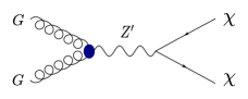
Figure 1: Production of dark matter through gluon fusion in the early Universe

In our set-up, the freeze-in occurs through the process depicted in Fig. 1. For a 1 + 2 $\rightarrow$ 3 + 4 process, the rate can be written as $R(T)=n_{\text{sm}}^{2}\langle\sigma v\rangle$, where $n_{\text{sm}}$ is the number density of the SM species and $\langle\sigma v\rangle$ is the thermal averaged production cross section. For a dark matter particle $i$, the rate reads

$$R(T)=\int f_{1}f_{2}\frac{E_{1}E_{2}\text{d}E_{1}\text{d}E_{2}~{}\text{d}\cos\theta_{12}}{1024\pi^{6}}\int|{\cal M}|_{i}^{2}\text{d}\Omega_{13}\,,$$ (10)

with $E_{1,2}$ and $f_{1,2}$ as the energy and the distribution function of the initial SM particles, $\theta_{12}$ as the angle between them, and $d\Omega_{13}$ as the solid angle between particles 1 and 3.

For the fermionic dark matter case,

$$\begin{split}\int|\mathcal{M}|_{\chi}^{2}~{}\text{d}\Omega_{13}&=2^{10}\pi~{}\frac{\alpha^{2}}{\Lambda^{4}}\frac{m_{\chi}^{2}}{M_{\text{$Z^{\prime}$}}^{4}}\frac{s^{3}(s-M_{\text{$Z^{\prime}$}}^{2})^{2}}{(s-M_{\text{$Z^{\prime}$}}^{2})^{2}+M_{\text{$Z^{\prime}$}}^{2}\Gamma_{\text{$Z^{\prime}$}}^{2}}\\ &\approx 2^{10}\pi~{}\frac{\alpha^{2}}{\Lambda^{4}}\frac{m_{\chi}^{2}}{M_{\text{$Z^{\prime}$}}^{4}}s^{3}\end{split}$$ (11)

For the Abelian dark matter case,

$$\begin{split}\int|\mathcal{M}|_{\text{\tiny{$X_{1}$}}}^{2}~{}\text{d}\Omega_{13}&=2^{10}\pi~{}\frac{\beta^{2}}{\Lambda^{4}}\frac{s^{3}}{M_{\text{$Z^{\prime}$}}^{4}}\frac{(s-4m_{\text{\tiny{$X_{1}$}}}^{2})(s-M_{\text{$Z^{\prime}$}}^{2})^{2}}{(s-M_{\text{$Z^{\prime}$}}^{2})^{2}+M_{\text{$Z^{\prime}$}}^{2}\Gamma_{\text{$Z^{\prime}$}}^{2}}\\ &\approx 2^{10}\pi~{}\frac{\beta^{2}}{\Lambda^{4}}\frac{1}{M_{\text{$Z^{\prime}$}}^{4}}s^{4}\end{split}$$ (12)

For the non-Abelian dark matter case,

$$\begin{split}\int|\mathcal{M}|_{\text{\tiny{$X_{N}$}}}^{2}\text{d}\Omega_{13}&=2^{12}\pi~{}\frac{\gamma^{2}}{\Lambda^{4}}\frac{s^{5}}{M_{\text{$Z^{\prime}$}}^{4}}\frac{(s-4m_{\text{\tiny{$X_{N}$}}}^{2})(s-M_{\text{$Z^{\prime}$}}^{2})^{2}}{(s-M_{\text{$Z^{\prime}$}}^{2})^{2}+M_{\text{$Z^{\prime}$}}^{2}\Gamma_{\text{$Z^{\prime}$}}^{2}}\\ &\approx 2^{12}\pi~{}\frac{\gamma^{2}}{\Lambda^{4}}\frac{1}{M_{\text{$Z^{\prime}$}}^{4}}s^{6}\end{split}$$ (13)

Above, $\Gamma_{\text{$Z^{\prime}$}}$ is the total width of $Z^{\prime}$ (see the Appendix for details); $s$ is the center-of-mass energy squared; and $m_{\chi},m_{\text{\tiny{$X_{1}$}}},m_{\text{\tiny{$X_{N}$}}}$, and $M_{\text{$Z^{\prime}$}}$ are the three types of dark matter and $Z^{\prime}$ masses, respectively. Note that we recover the Landau-Yang effect in the above expressions, though the pole enhancement studied in Ref. mambrinilast is not present in our case. Note also that the vectorial nature of the mediator has specific characteristics that we do not observe for other type of mediators. Importantly, we notice that once the pole is reached ($s=M_{\text{$Z^{\prime}$}}^{2}$), the production rate vanishes exactly – see Eqs. (11), (12), and (13). This is expected following the Landau-Yang theorem, which states that a massive spin-1 particle cannot decay into two massless spin-1 fields. This behavior is opposite of the traditional freeze-in scenario in which, on the contrary, the majority of dark matter is produced when the temperature of the thermal bath reaches $T\sim M_{\text{$Z^{\prime}$}}$ mambrinilast ; Blennow:2013jba .

We have integrated numerically the production rate, Eq. (10), considering the Bose-Einstein distributions of the gluons and the exact squared amplitudes of our three dark matter candidates. Our result is depicted in Fig.2.

We can obtain analytical approximations for the rates by assuming $\Gamma_{\text{$Z^{\prime}$}}\ll M_{\text{$Z^{\prime}$}}$ and $m_{\text{\tiny{DM}}}^{2}\ll s$:

$$R(T)\approx\left\{\begin{array}[]{rc}2\times 10^{2}~{}\dfrac{\alpha^{2}}{\Lambda^{4}}\dfrac{m_{\chi}^{2}}{M_{\text{$Z^{\prime}$}}^{4}}T^{10}~{}~{}~{}~{}(\text{fermionic DM})\\ \vskip 6.0pt plus 2.0pt minus 2.0pt\cr 10^{4}~{}\dfrac{\beta^{2}}{\Lambda^{4}M_{\text{$Z^{\prime}$}}^{4}}T^{12}~{}~{}~{}~{}~{}~{}(\text{Abelian DM})\\ \vskip 6.0pt plus 2.0pt minus 2.0pt\cr 2\times 10^{9}\dfrac{\gamma^{2}}{\Lambda^{4}M_{Z^{\prime}}^{4}}T^{16}~{}(\text{non-Abelian DM})\end{array}\right.$$ (14)

We also show in Fig. 2 our approximate solutions. In the inset of the figure, we show when they depart from the exact solutions. We can distinguish two regimes in which the approximations fail. First, let us consider when the temperature of the thermal bath is close to the mediator mass. In this case, the exact solutions are smaller than the approximate results as an effect of the nonvanishing mediator decay width. Even though the departure from approximations is small in this case, it carries a special feature of our set-up, emerging from the consequence of the Landau-Yang theorem in a thermal bath of gluons. The significant departure from approximations occurs at large $x\equiv M_{Z^{\prime}}/T$, due to a threshold effect, as for $T\ll m_{\text{\tiny{DM}}}$ the production rate is exponentially suppressed because only the high-energy tail of the initial states distribution function have sufficient energy to produce a DM pair, an effect that is not encapsulated in the analytical approximations.

Another typical characteristic of a longitudinal (“would-be Goldstone”) mediator appears in the generic expression for the rate. Indeed, the “light” mediator regime ($M_{\text{$Z^{\prime}$}}\ll T_{\text{\tiny{RH}}}$), and the “heavy” mediator regime ($M_{\text{$Z^{\prime}$}}\gg T_{\text{\tiny{RH}}}$) give the same dependence of the rate $R(T)$ on $M_{\text{$Z^{\prime}$}}$, and thus on temperature for a given nature of dark matter, as one can see from the Eq. (14) and Fig. 2. In fact, there exists only one main regime, independent of the mass of the $Z^{\prime}$ mediator for which the slope of the rate is constant until $T\sim m_{\text{\tiny{DM}}}$.

This can be understood by noting that only the longitudinal mode of $Z^{\prime}$ is exchanged, and hence it cannot feel any pole effect. The longitudinal component has its origin in the Goldstone mode of a nonlinear sigma model. The behavior of the amplitude squared is dominated by a term proportional to powers of $1/M_{\text{$Z^{\prime}$}}$. This happens because the Goldstone, which is the dominant mode exchanged in the DM production process, carries the $1/V$ factor arising from $U(1)^{\prime}$ breaking. This is similar to the gravitino production in supergravity in which the longitudinal mode, carrying a factor $1/m_{3/2}$ ($m_{3/2}$ being the gravitino mass), is generated in a high-scale supersymmetric scenario as was shown in Ref. gravitino .

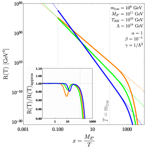
Figure 2: Rates for the fermionic, Abelian and non-Abelian DM (orange, green and blue lines, respectively). Solid lines represent the exact numerical computation while dashed lines represent the approximated results based on Eqs. (14). We fix $N_{\psi}=Q_{\psi}=1$ and $m_{\psi}=0.4~{}M_{\text{$Z^{\prime}$}}$ and $T_{\text{\tiny{MAX}}}=100~{}T_{\text{\tiny{RH}}}$ for illustrative purposes.

III.1 Dark matter freeze-in

For instantaneous reheating, the Universe is dominated by radiation and entropy is conserved. In this case,

$$\frac{\text{d}}{\text{d}t}=-H(T)T\frac{\text{d}}{\text{d}T},\hskip 14.22636pt\textrm{with}~{}~{}H(T)=\sqrt{\frac{g_{e}}{90}}\pi\frac{T^{2}}{M_{P}}$$ (15)

and Eq. (9) can be put in the familiar form

$$\frac{\text{d}Y}{\text{d}T}=-\frac{R(T)}{H~{}T~{}s}\,,\hskip 14.22636pt\textrm{for}~{}~{}T<T_{\text{\tiny{RH}}}$$ (16)

where $Y=\frac{n}{s}$ is the dark matter yield, $s=\frac{2\pi^{2}}{45}g_{s}T^{3}$ is the entropy density of the thermal bath with $g_{e,s}$ the energy and entropy density degrees of freedom, and $M_{P}\approx 2.4\times 10^{18}$ GeV is the reduced Planck mass.

However, once we consider noninstantaneous reheating, dark matter can be produced before the end of reheating. Indeed, as was shown in Refs. Giudice:2000ex ; Garcia:2017tuj , a rate with a dependence $R(T)\propto T^{n}$ for $n\geq 12$ enhances drastically the dark matter production before $T_{\text{\tiny{RH}}}$ if the reheating is considered as noninstantaneous. For instance, for $n=12$, the ratio of the relic abundance computed with the noninstantaneous reheating hypothesis ($\Omega h^{2}$) to the one with the instantaneous reheating hypothesis ($\Omega h^{2}_{\text{\tiny{RH}}}$) is $\Omega h^{2}/\Omega h^{2}_{\text{\tiny{RH}}}\simeq 0.4\times\dfrac{55}{6}\ln\left(\dfrac{T_{\text{\tiny{MAX}}}}{T_{\text{\tiny{RH}}}}\right)$ (where $T_{\text{\tiny{MAX}}}$ is the maximum temperature produced in the reheating process), whereas $\Omega h^{2}/\Omega h^{2}_{\text{\tiny{RH}}}\simeq 0.4\times\dfrac{8}{5}\left(\dfrac{n-5}{n-12}\right)\left(\dfrac{T_{\text{\tiny{MAX}}}}{T_{\text{\tiny{RH}}}}\right)^{n-12}$ for $n>12$ and $\Omega h^{2}/\Omega h^{2}_{\text{\tiny{RH}}}\sim 2$ for $n=10$. These ratios can be seen as “boost factors” from the reheating process and will be called $B^{n}_{F}\equiv\Omega h^{2}/\Omega h^{2}_{\text{\tiny{RH}}}$ from now on. After integrating Eq. (16) from $T_{\text{\tiny{MAX}}}$ until the present day, we deduce the parameter space leading to the relic abundance

$$\begin{split}&\frac{\Omega h^{2}}{0.12}\approx\left\{\begin{array}[]{lc}\left(\dfrac{B_{F}^{10}}{2}\right)\left(\dfrac{\alpha}{1}\right)^{2}\left(\dfrac{m_{\chi}}{6\times 10^{10}~{}{\rm GeV}}\right)^{3}\left(\dfrac{10^{14}~{}{\rm GeV}}{M_{\text{$Z^{\prime}$}}}\right)^{4}\left(\dfrac{10^{16}~{}{\rm GeV}}{\Lambda}\right)^{4}\left(\dfrac{T_{\text{\tiny{RH}}}}{10^{12}~{}{\rm GeV}}\right)^{5}\\ \vskip 6.0pt plus 2.0pt minus 2.0pt\cr\left(\dfrac{B_{F}^{12}}{21}\right)\left(\dfrac{\beta}{10^{-5}}\right)^{2}\left(\dfrac{m_{\text{\tiny{$X_{1}$}}}}{10^{9}~{}{\rm GeV}}\right)\left(\dfrac{10^{14}~{}{\rm GeV}}{M_{\text{$Z^{\prime}$}}}\right)^{4}\left(\dfrac{10^{16}~{}{\rm GeV}}{\Lambda}\right)^{4}\left(\dfrac{T_{\text{\tiny{RH}}}}{10^{13}~{}{\rm GeV}}\right)^{7}\\ \vskip 6.0pt plus 2.0pt minus 2.0pt\cr\left(\dfrac{B_{F}^{16}}{1.76\times 10^{8}}\right)\left(\dfrac{m_{\text{\tiny{$X_{N}$}}}}{2\times 10^{9}~{}{\rm GeV}}\right)\left(\dfrac{10^{14}~{}{\rm GeV}}{M_{\text{$Z^{\prime}$}}}\right)^{4}\left(\dfrac{10^{16}~{}{\rm GeV}}{\Lambda}\right)^{8}\left(\dfrac{T_{\text{\tiny{RH}}}}{10^{12}~{}{\rm GeV}}\right)^{11}\end{array}\right.\end{split}$$ (17)

where we set $\gamma=1/\Lambda^{2}$, and we consider $SU(2)$ as gauge group for the non-Abelian dark matter case.

Our results are summarized in Fig. 3, in which we plotted the parameter space allowed by the cosmological constraints in the plane $(m_{\text{\tiny{DM}}},\Lambda)$ for the three natures of dark matter considered in this work and for $T_{\text{\tiny{RH}}}=10^{10}~{}\text{GeV}$ and $T_{\text{\tiny{MAX}}}=100~{}T_{\text{\tiny{RH}}}$. To compute the relic abundance numerically, we did not assume instantaneous reheating. Instead, using the method developed in Ref. Garcia:2017tuj , we assumed that an inflaton $\phi$ decays into radiation with a rate $\Gamma_{\phi}$ and that the DM particles are created and annihilated into radiation of density $\rho_{\text{R}}$ with a thermal-averaged cross section times velocity $\langle\sigma v\rangle$. The corresponding energy and number densities satisfy the differential equations Chung:1998rq ; Giudice:2000ex

$$\frac{\text{d}n_{\text{\tiny{DM}}}}{\text{d}t} = -3H\,n_{\text{\tiny{DM}}}-\langle\sigma v\rangle\left[n_{\text{\tiny{DM}}}^{2}-(n_{\text{\tiny{DM}}}^{\text{eq}})^{2}\right]\,,$$

$$\frac{\text{d}\rho_{\text{R}}}{\text{d}t} = -4H\,\rho_{\text{R}}+\Gamma_{\phi}\,\rho_{\phi}+2\langle\sigma v\rangle\langle E_{\text{\tiny{DM}}}\rangle\left[n_{\text{\tiny{DM}}}^{2}-(n_{\text{\tiny{DM}}}^{\text{eq}})^{2}\right]\,,$$

$$\frac{\text{d}\rho_{\phi}}{\text{d}t} = -3H\,\rho_{\phi}-\Gamma_{\phi}\,\rho_{\phi}\,,$$ (18)

with $\langle E_{\text{\tiny{DM}}}\rangle$ the mean energy of the dark matter. The Hubble expansion parameter $H$ is given by $H^{2}=\frac{1}{3M_{P}^{2}}(\rho_{\phi}+\rho_{\text{R}}+\rho_{\text{\tiny{DM}}})$, and its dependence in temperature is quite complex between $T_{\text{\tiny{MAX}}}$ and $T_{\text{\tiny{RH}}}$ because of the composition of the Universe (mixed between a decaying inflaton compensated by an increasing radiation).

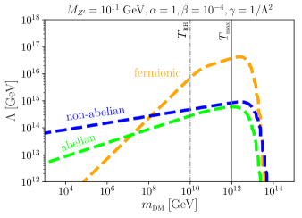
Figure 3: Relic density curves for the fermionic (orange dashed line), Abelian (green dashed line) and non-Abelian (blue dashed line) dark matter.

We can see that our analytical expressions in Eq. (17) give an impressively good approximation. Indeed, the right amount of relic abundance planck is obtained (in the fermionic case) for $m_{\chi}=10^{6}$ GeV, $T_{\text{\tiny{RH}}}=10^{10}$ GeV, $M_{\text{$Z^{\prime}$}}=10^{11}$ GeV, and $\Lambda\simeq 8\times 10^{12}$ GeV, in perfect agreement with Fig. 3. The slopes of the curves depicted in Fig. 3 correspond also perfectly with the ones predicted by our analytical solution in Eq. (17): it follows a line $\Lambda\propto m_{\text{\tiny{DM}}}^{3/4}$ ($m_{\text{\tiny{DM}}}^{1/4}$, $m_{\text{\tiny{DM}}}^{1/8}$) for fermionic (Abelian, non-Abelian) for $m_{\text{\tiny{DM}}}<T_{\text{\tiny{MAX}}}$.

Without entering too much into detail, there is an interesting feature in the change of slope between $T_{\text{\tiny{RH}}}$ and $T_{\text{\tiny{MAX}}}$ in the fermionic dark matter case. This is a novel feature that was not treated in Ref. Garcia:2017tuj nor Ref. mambrinilast . Indeed, in the case in which dark matter is heavier than $T_{\text{\tiny{RH}}}$, there is still a possibility to produce it as long as $m_{\text{\tiny{DM}}}\lesssim T_{\text{\tiny{MAX}}}$. If the temperature dependence of the rate is small enough (fermionic case), most of the DM density is produced at the lowest scale available, and we notice a change of slope in the curve giving the correct relic density. It is worth commenting that, due to statistical distribution, the production rate does not vanish completely when $T\lesssim m_{\text{\tiny{DM}}}$, which explains why the DM production window is still open when $m_{\text{\tiny{DM}}}>T_{\text{\tiny{MAX}}}$. Therefore, in this regime, a small effective scale $\Lambda$ is required to compensate the thermal suppression of the rate, as one can see in Fig.3.

Moreover, a quick look at Fig.3 shows to what extent the allowed parameter space is technically natural. Indeed, for a very large range of the DM mass, from $\mathcal{O}$(TeV) to $T_{\text{\tiny{RH}}}$, values of the beyond SM scale $\Lambda$ range from $T_{\text{\tiny{RH}}}$ to GUT/string scale and can still populate the Universe with the correct relic abundance. This means that the heavy spectrum of masses above the reheating temperature $T_{\text{\tiny{RH}}}$ generates naturally small couplings of an invisible $Z^{\prime}$ to the SM bath to satisfy the cosmological constraints through the freeze-in process. This constitutes one of the most important observations of our work.

IV IV. toward a microscopic approach

As mentioned earlier, we consider processes happening at a temperature below the $U(1)^{\prime}$ phase transition scale. We have also assumed that the radial component of the complex scalar that breaks $U(1)^{\prime}$ is way too heavy compared to the corresponding VEV ($V$). Then, $Z^{\prime}$ is primarily longitudinal absorbing the axion field ($a$), and the effective Lagrangian containing $Z^{\prime}$ realizes the gauge symmetry nonlinearly à la Stueckelberg. Now, we attempt to look deep inside the effective GCS vertices searching for microscopic details. Importantly, the masses of the loop fermions ($\Psi$) generating the GCS couplings, as shown in Fig. 4, must be invariant both under the SM and the $U(1)^{\prime}$ gauge symmetries to ensure that the induced low-energy GCS operators are gauge invariant. One can, in fact, write the microscopic (gauge-invariant) Lagrangian introducing pairs of heavy fermions ($\Psi$) that are vectorlike with respect to the SM group, but necessarily chiral under $U(1)^{\prime}$. This generates the effective Lagrangian (5) at energies below the $U(1)^{\prime}$ breaking scale,

$$\begin{split}{\cal L}=&{\cal L}_{\text{SM}}+\frac{1}{2}(\partial_{\mu}a-M_{Z^{\prime}}Z^{\prime}_{\mu})^{2}-M_{i}~{}\overline{\Psi}^{i}_{L}e^{i(q_{L}-q_{R})\frac{a}{V}}\Psi^{i}_{R}\\ &+i\overline{\Psi}^{i}_{L}\gamma^{\mu}(\partial_{\mu}-i\frac{\tilde{g}}{2}q_{L}^{i}Z^{\prime}_{\mu})\Psi^{i}_{L}+i\overline{\Psi}^{i}_{R}\gamma^{\mu}(\partial_{\mu}-i\frac{\tilde{g}}{2}q_{R}^{i}Z^{\prime}_{\mu})\Psi^{i}_{R}\end{split}$$ (19)

which is manifestly invariant under the (nonlinear) $U(1)^{\prime}$ transformation of parameter $\alpha$,

$$\Psi^{i}_{R}\rightarrow\Psi^{i}_{R}e^{i\frac{\tilde{g}}{2}q_{R}\alpha}~{};~{}~{}~{}~{}\Psi^{i}_{L}\rightarrow\Psi^{i}_{L}e^{i\frac{\tilde{g}}{2}q_{L}\alpha}$$

$$Z^{\prime}_{\mu}\rightarrow Z^{\prime}_{\mu}+\partial_{\mu}\alpha~{};~{}~{}~{}~{}a\rightarrow a+\frac{\tilde{g}}{2}V~{}\alpha\equiv a+M_{Z^{\prime}}~{}\alpha$$

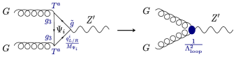
Figure 4: Triangle diagram containing heavy chiral fermions $\Psi_{i}$ (left panel) and the resulting effective vertex at low energy (right panel).

From the Lagrangian in Eq. (19), we compute the triangle loops shown in Fig. 4 and integrate out the heavy fermions. We then obtain the same effective Lagrangian as in Eq. (5), but now we can express the effective coupling of the dimension-6 Lagrangian in terms of the parameters of the microscopical theory. In agreement with Ref. Dudas:2013sia , we obtain

$${\cal L}_{\text{loop}}=\frac{1}{\Lambda_{\text{loop}}^{2}}\partial^{\alpha}Z^{\prime}_{\alpha}\epsilon^{\mu\nu\rho\sigma}\mathrm{Tr}[G^{a}_{\mu\nu}G^{a}_{\rho\sigma}],$$ (20)

with

$$\frac{1}{\Lambda_{\text{loop}}^{2}}=\frac{g_{3}^{2}~{}\tilde{g}}{96\pi^{2}}\sum_{i}\frac{q_{L}^{i}-q_{R}^{i}}{M_{\Psi_{i}}^{2}}\mathrm{Tr}[T^{a}T^{a}].$$ (21)

Defining for simplicity $\sum_{i}\frac{q_{L}^{i}-q_{R}^{i}}{M_{\Psi_{i}}^{2}}\mathrm{Tr}[T^{a}T^{a}]=\frac{N_{\Psi}Q_{\Psi}}{M_{\Psi}^{2}}$ (which corresponds to a set of $N_{\Psi}$ fermions of effective charges $Q_{\Psi}$ and masses $M_{\Psi}$) we obtain $\Lambda_{\text{loop}}\simeq\frac{50}{\sqrt{N_{\Psi}Q_{\Psi}}}\frac{M_{\Psi}}{\sqrt{\tilde{g}}}$. We can now reexpress the production rates in Eqs. (14) in terms of the fundamental parameters of the microscopic theory. For the fermionic dark matter case, we then have

$$R(T)\simeq 5\times 10^{-4}\left(\frac{\alpha~{}N_{\Psi}Q_{\Psi}}{y_{\Psi}^{2}\tilde{g}}\right)^{2}\frac{m_{\chi}^{2}}{V^{8}}T^{10}$$ (22)

where we defined $M_{\Psi}=y_{\Psi}V$ and $M_{Z^{\prime}}=\frac{\tilde{g}}{2}V$. Solving Eq. (16) gives (with all mass dimensional parameters in GeV units)

$$\dfrac{\Omega h^{2}}{0.12}\simeq\left(\dfrac{B_{F}^{10}}{2}\right)\left(\frac{\alpha N_{\Psi}Q_{\Psi}}{\tilde{g}y_{\Psi}^{2}}\right)^{2}\left(\frac{m_{\chi}}{10^{10}}\right)^{3}\left(\frac{T_{\text{RH}}}{10^{12}}\right)^{5}\left(\frac{10^{14}}{V}\right)^{8}.$$ (23)

We could keep $V$ as a free fundamental parameter of the model, which is determined by the potential of the Higgs responsible for the extra $U(1)^{\prime}$ breaking. However, to be more complete, we investigated UV scenarios in which $V$ is determined as an intermediate scale by the unification condition of the gauge coupling constants, in $SO(10)$ GUT constructions (as an example).

Indeed, in such set-ups, the $SO(10)$ group is not directly broken into the SM in one step but goes through an intermediate gauge group $G_{\text{int}}$ like $SO(10)\rightarrow G_{\text{int}}\rightarrow SU(3)_{c}\times SU(2)_{L}\times U(1)_{Y}$. The scale $M_{\text{int}}$ at which the intermediate gauge group is broken is fixed by the unification condition $g_{1}=g_{2}=g_{3}$ at a higher unified scale. It was shown in Refs. Mambrini:2013iaa (at one loop) and 2loops (at two loops) that $V=M_{\rm int}$ can range from $10^{9}$ to $10^{15}$ GeV depending on $G_{\text{int}}$ and the representation in which the Higgs field responsible for $G_{\text{int}}$ breaking lies. We show in Fig. 5 the parameter space providing the correct relic density for our fermionic dark matter candidate in several intermediate scenarios. Here, we take $V=M_{\Psi}=M_{\text{int}}$, which is a reasonable approximation. The numerical results, obtained by solving the complete set of Boltzmann equations, Eq. (18), and numerical integration of the rate, Eq. (10), are in perfect agreement with our analytical solution Eq. (23).

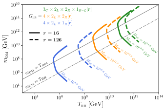
Figure 5: Relic density curves for the fermionic DM case in several $SO(10)$ breaking schemes and for different representations [$\boldmath{r}$] for the Higgs field responsible for intermediate scale breaking. We take $N_{\Psi}=Q_{\Psi}=y_{\Psi}=1$ for illustrative purposes.

We observe that in these unified scenarios DM density corresponding to the Planck measurements planck can be directly produced from annihilation of SM particles even if the mediator $Z^{\prime}$ is extremely heavy with no SM particles charged under the extra $U(1)^{\prime}$. The effective couplings of the thermal bath to $Z^{\prime}$ are being generated through the GCS interactions.

Figure 5 highlights the natural relation between the parameters of the theory $M_{\text{int}}\sim T_{\text{\tiny{MAX}}}\sim 10^{2}~{}T_{\text{\tiny{RH}}}\sim 10^{2}~{}m_{\text{\tiny{DM}}}$ corresponding to the correct DM relic abundance. Therefore, the intermediate scale in such unified constructions could be closely related to the inflaton mass as one expects it to be of the order of the maximum temperature reached by the SM thermal bath. The large hierarchy between these scales and the SM electroweak VEV naturally provides the suppressed DM-SM effective coupling required to produce the correct DM density nonthermally via the freeze-in mechanism.

Though the heavy colored fermions $\Psi$ are cosmologically stable, their very small number density owing to their heaviness ($\sim 10^{14}$ GeV) keeps them hidden as benign. In principle, these states contribute to the running of $g_{3}$, but they are kicked into life so late that the nonstandard modification of running during the remaining phase up to the GUT scale is inconsequential.

If, however, the $\Psi$ states additionally have SM hypercharge, there is a nontrivial twist. Through loop contributions, they would induce a kinetic mixing term like $\delta B^{\mu\nu}Z^{\prime}_{\mu\nu}$, which would ascribe the kinetically diagonal $Z^{\prime}$ with a small, proportional to $\delta$, coupling with the SM fermion $f$. This would allow the direct s-channel production of DM from $f$ annihilation as follows: $\bar{f}+f\rightarrow Z^{\prime}\rightarrow\text{DM}+\text{DM}$. Note that the natural size of $\delta$ is a loop factor times a logarithm of the ratio of two scales, so $\delta\sim 10^{-4}$ is a representative number. If $M_{Z^{\prime}}<T_{\rm MAX}$, then through $Z^{\prime}$, the DM would obviously be in thermal equilibrium with the SM. But this does not constitute the FIMP or freeze-in scenario we are pursuing here. On the other hand, if $M_{Z^{\prime}}>T_{\rm MAX}$, the above-mentioned tree-level $s$-channel annihilation, as shown in Mambrini:2013iaa , would be the dominating process. The GCS coupling-induced process we advocated in this paper would then be a subleading one. The importance of our analysis lies in the fact that even if the heavy $\Psi$ states do not carry the SM hypercharge and the kinetic mixing is absent, the novel mechanism triggered by the GCS interaction can still explain the relic DM abundance albeit for an inaccessibly high-mass range of both the DM and its portals.

V V. Conclusion

We have shown that a dark (very) massive $Z^{\prime}$, not charged under the SM gauge group, can successfully play the role of a mediator between the visible and the dark sectors even if the corresponding $U(1)^{\prime}$ breaking scale lies far above the maximum temperature of the Universe. Pair annihilation of SM gauge bosons, proceeding through triangle loops containing heavy fermions through this $Z^{\prime}$ portal, can produce a cosmologically agreeable amount of DM. These types of effective couplings between the SM gauge bosons and $Z^{\prime}$ find inherent justification in an anomaly-free set-up in which Chern-Simons (more precisely, the GCS type discussed in the beginning) terms are generated through the anomaly cancellation mechanism.

The large effective scale of the GCS operators is responsible for the weakness of the DM-SM interaction strength without invoking unnaturally small couplings as is often required in the context of freeze-in. The large dependence of the production rate on temperature indicates that the majority of DM is produced during the initial moments of reheating. Subsequently, the reheating process itself lends important consequences to the computation of DM production. Moreover, the assertion that the $U(1)^{\prime}$ breaking scale lies far above the reheating temperature implies that only the longitudinal mode (axion à la the Stueckelberg formalism) of the $Z^{\prime}$ contributes to the production process, rendering its phenomenology very particular in comparison with other type of mediators. The prominence of the longitudinal mode is also consistent with how $Z^{\prime}$ is coupled via GCS interaction. Such a scenario can be embedded in a unified $SO(10)$ framework in which the $Z^{\prime}$ mass scale represents an intermediate breaking stage of $SO(10)$.

Acknowledgments: The authors want to thank especially E. Dudas for very insightful discussions. This research has been supported by the (Indo-French) CEFIPRA/IFCPAR Project No. 5404-2. Support from CNRS LIA-THEP and the INFRE-HEPNET of CEFIPRA/IFCPAR is also acknowledged. G.B. acknowledges support of the J.C. Bose National Fellowship from the Department of Science and Technology, Government of India (SERB Grant No. SB/S2/JCB-062/2016). M.D. acknowledges support from the Brazilian Ph.D. program “Ciências sem Fronteiras” – CNPQ Process No. 202055/2015-9. This work was also supported by the France-US PICS no. 06482, PICS MicroDark. M. D. and Y. M. acknowledge partial support from the European Union Horizon 2020 research and innovation programme under the Marie Sklodowska-Curie: RISE InvisiblesPlus (Grant No 690575) and the ITN Elusives (Grant No 674896).

Appendix

VI noninstantaneous reheating: analytical estimations

As the reheating is not an instantaneous process, the inflaton dominates the energy density of the Universe at some stage and we have a different relation between time and temperature Giudice:2000ex

$$\frac{\text{d}}{\text{d}t}=-\frac{3}{8}H(T)T\frac{\text{d}}{\text{d}T},~{}~{}\textrm{with}~{}~{}H(T)=\frac{d}{c}\sqrt{\frac{5g_{e}^{2}}{72g_{\text{\tiny{RH}}}}}\pi\frac{T^{4}}{T_{\text{\tiny{RH}}}^{2}M_{P}},$$ (24)

with $g_{\text{\tiny{RH}}}=g_{e}(T_{\text{\tiny{RH}}})$.

We emphasize that while the inflaton dominates, we have $T\propto a^{-3/8}$ instead of $a^{-1}$ as in the radiation-dominated era, with $a$ the expansion scale factor.

It is convenient to define the dimensionless quantity $\mathcal{N}_{\phi}\equiv\rho_{\phi}/T_{\text{\tiny{RH}}}a^{3}$ Giudice:2000ex , with $\rho_{\phi}$ the energy density of the inflaton field. It remains constant before the end of reheating, with a value given by $\mathcal{N}_{\phi}^{I}\propto(\frac{T_{\text{\tiny{MAX}}}}{T_{\text{\tiny{RH}}}})^{8}$.

We notice that, by using Eq. (24), Eq. (9) can be put in the form

$$\frac{\text{d}Y_{\text{\tiny{ID}}}}{\text{d}T}=-\frac{8}{3}\frac{R(T)}{H~{}T~{}\epsilon},\hskip 14.22636pt\textrm{for}~{}~{}T_{\text{\tiny{RH}}}<T<T_{\text{\tiny{MAX}}}$$ (25)

where the yield in the inflaton-dominated era is defined as the dimensionless and comoving parameter $Y_{\text{\tiny{ID}}}\equiv n/\epsilon$ and $\epsilon$ is defined as

$$\epsilon\equiv\mathcal{N}_{\phi}^{I}a^{-3}=\frac{5d^{2}g_{e}^{2}}{96c^{2}g_{\text{\tiny{RH}}}T_{\text{\tiny{RH}}}^{5}}T^{8}.$$ (26)

By solving Eq. (25), we can find the contribution of the noninstantaneous heating process to the relic density and define the boost factor discussed in Sec. III.

VII Decay width

We present the decay width used in the computation of the production rate. Allowing the $Z^{\prime}$ to decay into $N_{\psi}$ dark heavy fermions $\psi$ (with only vectorial coupling) of charge $Q_{\psi}$ and mass $m_{\psi}$, the total decay width is given by

$$\Gamma_{Z^{\prime}}=\frac{M_{\text{$Z^{\prime}$}}}{12\pi}N_{\psi}Q_{\psi}^{2}\sqrt{1-\frac{4m_{\psi}^{2}}{M_{\text{$Z^{\prime}$}}^{2}}}\Big{(}1+\frac{2m_{\psi}^{2}}{M_{\text{$Z^{\prime}$}}^{2}}\Big{)}+\Gamma_{\text{$Z^{\prime}$}\rightarrow\text{DM}},$$ (27)

where

$$\Gamma_{\text{$Z^{\prime}$}\rightarrow\text{DM}}=\frac{M_{\text{$Z^{\prime}$}}}{12\pi}\times\left\{\begin{array}[]{rc}\alpha^{2}\Big{(}1-\frac{4m_{\chi}^{2}}{M_{\text{$Z^{\prime}$}}^{2}}\Big{)}^{3/2}~{}(\text{fermionic DM})\\ \vskip 6.0pt plus 2.0pt minus 2.0pt\cr\frac{\beta^{2}}{2}\frac{M_{\text{$Z^{\prime}$}}^{2}}{m_{\text{\tiny{$X_{1}$}}}^{2}}\Big{(}1-\frac{4m_{\text{\tiny{$X_{1}$}}}^{2}}{M_{\text{$Z^{\prime}$}}^{2}}\Big{)}^{5/2}~{}~{}~{}(\text{Abelian DM})\\ \vskip 6.0pt plus 2.0pt minus 2.0pt\cr 0~{}~{}~{}~{}~{}~{}~{}~{}~{}(\text{non-Abelian DM})\end{array}\right.$$ (28)

The decay width of $Z^{\prime}$ into non-Abelian DM vanishes identically because of the nature of the coupling.

References

- (1) P. A. R. Ade et al. [Planck Collaboration], Astron. Astrophys. 594, A13 (2016) [arXiv:1502.01589 [astro-ph.CO]].
- (2) E. Aprile et al. [XENON100 Collaboration], Phys. Rev. Lett. 109 (2012) 181301 [arXiv:1207.5988 [astro-ph.CO]].
- (3) D. S. Akerib et al. [LUX Collaboration], Phys. Rev. Lett. 118 (2017) no.2, 021303 [arXiv:1608.07648 [astro-ph.CO]].
- (4) C. Fu et al. [PandaX-II Collaboration], Phys. Rev. Lett. 118, no. 7, 071301 (2017) [arXiv:1611.06553 [hep-ex]].
- (5) J. A. Casas, D. G. Cerdeño, J. M. Moreno and J. Quilis, JHEP 1705 (2017) 036 doi:10.1007/JHEP05(2017)036 [arXiv:1701.08134 [hep-ph]]. A. Djouadi, O. Lebedev, Y. Mambrini and J. Quevillon, Phys. Lett. B 709 (2012) 65 doi:10.1016/j.physletb.2012.01.062 [arXiv:1112.3299 [hep-ph]]; A. Djouadi, A. Falkowski, Y. Mambrini and J. Quevillon, Eur. Phys. J. C 73 (2013) no.6, 2455 doi:10.1140/epjc/s10052-013-2455-1 [arXiv:1205.3169 [hep-ph]]; O. Lebedev, H. M. Lee and Y. Mambrini, Phys. Lett. B 707 (2012) 570 doi:10.1016/j.physletb.2012.01.029 [arXiv:1111.4482 [hep-ph]]; Y. Mambrini, Phys. Rev. D 84 (2011) 115017 doi:10.1103/PhysRevD.84.115017 [arXiv:1108.0671 [hep-ph]].
- (6) J. Ellis, A. Fowlie, L. Marzola and M. Raidal, arXiv:1711.09912 [hep-ph]. G. Arcadi, Y. Mambrini and F. Richard, JCAP 1503 (2015) 018 [arXiv:1411.2985 [hep-ph]]; J. Kearney, N. Orlofsky and A. Pierce, arXiv:1611.05048 [hep-ph]; M. Escudero, A. Berlin, D. Hooper and M. X. Lin, JCAP 1612 (2016) 029 doi:10.1088/1475-7516/2016/12/029 [arXiv:1609.09079 [hep-ph]].
- (7) A. Alves, S. Profumo and F. S. Queiroz, JHEP 1404 (2014) 063 doi:10.1007/JHEP04(2014)063 [arXiv:1312.5281 [hep-ph]]. O. Lebedev and Y. Mambrini, Phys. Lett. B 734 (2014) 350 [arXiv:1403.4837 [hep-ph]]; G. Arcadi, Y. Mambrini, M. H. G. Tytgat and B. Zaldivar, JHEP 1403 (2014) 134 [arXiv:1401.0221 [hep-ph]]; O. Lebedev and Y. Mambrini, Phys. Lett. B 734 (2014) 350 doi:10.1016/j.physletb.2014.05.025 [arXiv:1403.4837 [hep-ph]].
- (8) G. Arcadi, M. Dutra, P. Ghosh, M. Lindner, Y. Mambrini, M. Pierre, S. Profumo and F. S. Queiroz, Eur. Phys. J. C 78 (2018) no.3, 203 doi:10.1140/epjc/s10052-018-5662-y [arXiv:1703.07364 [hep-ph]].
- (9) L. J. Hall, K. Jedamzik, J. March-Russell and S. M. West, JHEP 1003 (2010) 080 [arXiv:0911.1120 [hep-ph]]; X. Chu, T. Hambye and M. H. G. Tytgat, JCAP 1205 (2012) 034 [arXiv:1112.0493 [hep-ph]]; X. Chu, Y. Mambrini, J. Quevillon and B. Zaldivar, JCAP 1401 (2014) 034 [arXiv:1306.4677 [hep-ph]].
- (10) N. Bernal, M. Heikinheimo, T. Tenkanen, K. Tuominen and V. Vaskonen, Int. J. Mod. Phys. A 32 (2017) no.27, 1730023 doi:10.1142/S0217751X1730023X [arXiv:1706.07442 [hep-ph]].
- (11) Z. G. Berezhiani, A. D. Dolgov and R. N. Mohapatra, Phys. Lett. B 375 (1996) 26 doi:10.1016/0370-2693(96)00219-5 [hep-ph/9511221]; P. Adshead, Y. Cui and J. Shelton, JHEP 1606 (2016) 016 doi:10.1007/JHEP06(2016)016 [arXiv:1604.02458 [hep-ph]]; E. Hardy and J. Unwin, JHEP 1709 (2017) 113 doi:10.1007/JHEP09(2017)113 [arXiv:1703.07642 [hep-ph]].
- (12) N. Bernal, M. Dutra, Y. Mambrini, K. A. Olive, M. Peloso and M. Pierre, arXiv:1803.01866 [hep-ph].
- (13) M. Garny, A. Palessandro, M. Sandora and M. S. Sloth, JCAP 1802, no. 02, 027 (2018) doi:10.1088/1475-7516/2018/02/027 [arXiv:1709.09688 [hep-ph]].
- (14) M. Garny, M. Sandora and M. S. Sloth, Phys. Rev. Lett. 116 (2016) no.10, 101302 doi:10.1103/PhysRevLett.116.101302 [arXiv:1511.03278 [hep-ph]].
- (15) A. Biswas, D. Borah and A. Dasgupta, arXiv:1805.06903 [hep-ph].
- (16) Y. Mambrini, K. A. Olive, J. Quevillon and B. Zaldivar, Phys. Rev. Lett. 110 (2013) no.24, 241306 [arXiv:1302.4438 [hep-ph]];
- (17) Y. Mambrini, N. Nagata, K. A. Olive, J. Quevillon and J. Zheng, Phys. Rev. D 91 (2015) no.9, 095010 doi:10.1103/PhysRevD.91.095010 [arXiv:1502.06929 [hep-ph]]; Y. Mambrini, N. Nagata, K. A. Olive and J. Zheng, Phys. Rev. D 93 (2016) no.11, 111703 doi:10.1103/PhysRevD.93.111703 [arXiv:1602.05583 [hep-ph]].
- (18) P. Anastasopoulos, M. Bianchi, E. Dudas and E. Kiritsis, JHEP 0611 (2006) 057 doi:10.1088/1126-6708/2006/11/057 [hep-th/0605225].
- (19) J. A. Dror, R. Lasenby and M. Pospelov, Phys. Rev. D 96 (2017) no.7, 075036 doi:10.1103/PhysRevD.96.075036 [arXiv:1707.01503 [hep-ph]]; F. Kahlhoefer, K. Schmidt-Hoberg, T. Schwetz and S. Vogl, JHEP 1602 (2016) 016 doi:10.1007/JHEP02(2016)016 [arXiv:1510.02110 [hep-ph]]; Y. Cui and F. D’Eramo, Phys. Rev. D 96 (2017) no.9, 095006 doi:10.1103/PhysRevD.96.095006 [arXiv:1705.03897 [hep-ph]]; J. A. Dror, R. Lasenby and M. Pospelov, Phys. Rev. Lett. 119 (2017) no.14, 141803 doi:10.1103/PhysRevLett.119.141803 [arXiv:1705.06726 [hep-ph]].
- (20) A. Ismail, A. Katz and D. Racco, JHEP 1710 (2017) 165 doi:10.1007/JHEP10(2017)165 [arXiv:1707.00709 [hep-ph]]; G. Arcadi, P. Ghosh, Y. Mambrini, M. Pierre and F. S. Queiroz, JCAP 1711 (2017) no.11, 020 doi:10.1088/1475-7516/2017/11/020 [arXiv:1706.04198 [hep-ph]]; S. M. Choi, Y. Hochberg, E. Kuflik, H. M. Lee, Y. Mambrini, H. Murayama and M. Pierre, JHEP 1710 (2017) 162 doi:10.1007/JHEP10(2017)162 [arXiv:1707.01434 [hep-ph]].
- (21) Y. Farzan and A. R. Akbarieh, JCAP 1411 (2014) no.11, 015 doi:10.1088/1475-7516/2014/11/015 [arXiv:1408.2950 [hep-ph]].
- (22) G. F. Giudice, E. W. Kolb and A. Riotto, Phys. Rev. D 64 (2001) 023508 doi:10.1103/PhysRevD.64.023508 [hep-ph/0005123].
- (23) M. A. G. Garcia, Y. Mambrini, K. A. Olive and M. Peloso, Phys. Rev. D 96 (2017) no.10, 103510 doi:10.1103/PhysRevD.96.103510 [arXiv:1709.01549 [hep-ph]].
- (24) K. Benakli, Y. Chen, E. Dudas and Y. Mambrini, Phys. Rev. D 95 (2017) no.9, 095002 doi:10.1103/PhysRevD.95.095002 [arXiv:1701.06574 [hep-ph]]; E. Dudas, Y. Mambrini and K. Olive, Phys. Rev. Lett. 119 (2017) no.5, 051801 doi:10.1103/PhysRevLett.119.051801 [arXiv:1704.03008 [hep-ph]]; E. Dudas, T. Gherghetta, Y. Mambrini and K. A. Olive, Phys. Rev. D 96 (2017) no.11, 115032 doi:10.1103/PhysRevD.96.115032 [arXiv:1710.07341 [hep-ph]]; E. Dudas, T. Gherghetta, K. Kaneta, Y. Mambrini and K. A. Olive, arXiv:1805.07342 [hep-ph].
- (25) E. Dudas, L. Heurtier, Y. Mambrini and B. Zaldivar, JHEP 1311 (2013) 083 doi:10.1007/JHEP11(2013)083 [arXiv:1307.0005 [hep-ph]].
- (26) E. Dudas, Y. Mambrini, S. Pokorski and A. Romagnoni, JHEP 1210 (2012) 123 doi:10.1007/JHEP10(2012)123 [arXiv:1205.1520 [hep-ph]]; Y. Mambrini, JCAP 0912 (2009) 005 doi:10.1088/1475-7516/2009/12/005 [arXiv:0907.2918 [hep-ph]]; E. Dudas, Y. Mambrini, S. Pokorski and A. Romagnoni, JHEP 0908 (2009) 014 doi:10.1088/1126-6708/2009/08/014 [arXiv:0904.1745 [hep-ph]].
- (27) G. Bélanger, J. Da Silva and H. M. Tran, Phys. Rev. D 95 (2017) no.11, 115017 doi:10.1103/PhysRevD.95.115017 [arXiv:1703.03275 [hep-ph]]. J. L. Feng, J. Smolinsky and P. Tanedo, Phys. Rev. D 93 (2016) no.11, 115036 Erratum: [Phys. Rev. D 96 (2017) no.9, 099903] doi:10.1103/PhysRevD.93.115036, 10.1103/PhysRevD.96.099903 [arXiv:1602.01465 [hep-ph]]. Y. Mambrini, JCAP 1107 (2011) 009 doi:10.1088/1475-7516/2011/07/009 [arXiv:1104.4799 [hep-ph]].
- (28) M. Blennow, E. Fernandez-Martinez and B. Zaldivar, JCAP 1401 (2014) 003 doi:10.1088/1475-7516/2014/01/003 [arXiv:1309.7348 [hep-ph]].
- (29) D. J. H. Chung, E. W. Kolb and A. Riotto, Phys. Rev. D 60 (1999) 063504 doi:10.1103/PhysRevD.60.063504 [hep-ph/9809453].
- (30) V. De Luca, A. Mitridate, M. Redi, J. Smirnov and A. Strumia, Phys. Rev. D 97 (2018) no.11, 115024 doi:10.1103/PhysRevD.97.115024 [arXiv:1801.01135 [hep-ph]].
- (31) P. F. Smith, J. R. J. Bennett, G. J. Homer, J. D. Lewin, H. E. Walford and W. A. Smith, Nucl. Phys. B 206 (1982) 333. doi:10.1016/0550-3213(82)90271-1.