Topological Dualities in the Ising Model

Abstract.

We relate two classical dualities in low-dimensional quantum field theory: Kramers-Wannier duality of the Ising and related lattice models in $2$ dimensions, with electromagnetic duality for finite gauge theories in $3$ dimensions. The relation is mediated by the notion of boundary field theory: Ising models are boundary theories for pure gauge theory in one dimension higher. Thus the Ising order/disorder operators are endpoints of Wilson/’t Hooft defects of gauge theory. Symmetry breaking on low-energy states reflects the multiplicity of topological boundary states. In the process we describe lattice theories as (extended) topological field theories with boundaries and domain walls. This allows us to generalize the duality to non-abelian groups; finite, semi-simple Hopf algebras; and, in a different direction, to finite homotopy theories in arbitrary dimension.

In quantum field theory and statistical mechanics, the $2$-dimensional Ising model has earned the double distinction of being the first discrete model to exhibit, against expectations, phase transitions in the large volume limit [P], and the first non-trivial one to be solved explicitly [O]. It is the simplest lattice sigma-model (in apocryphal terminology) with only nearest-neighbor interactions, and depends on a single parameter, physically interpreted as the temperature $T$, and encoded as the reciprocal $\beta=1/kT$ (with Boltzmann’s $k$). Nowadays, detailed treatments can be found in graduate textbooks [ID, C]. The present paper is our mathematical attempt to understand some features of the story and locate them within the algebraic structures of topological quantum field theory (TQFT).

The Ising model assigns two possible states (spins valued in $\pm 1$) to each node of a $2$-dimensional lattice. Equal spins for nearby nodes are probabilistically favored, strongly or weakly, according to $\beta$. For a very large lattice, the system exhibits two phases: a ferromagnetic phase at low temperature, where the spins are mostly aligned, with one sign dominating; and a paramagnetic phase at high temperature, where regions of spins of both signs co-exist. The model also has a $2$D Euclidean (lattice) quantum field theory interpretation, with a space of states $\mathcal{H}$ assigned to any “latticed” circle (subdivided into edges and nodes). Specifically, $\mathcal{H}$ is the space of functions on the set of possible independent spin assignments to the nodes, and is acted upon by the transfer matrix, the analogue of the exponentiated negative-signed Hamiltonian on a cylindrical space-time. At low temperature, its top eigenvalue is achieved on the two aligned spin states, the two $\delta$-functions on the constant maps to $\{\pm 1\}$. At high temperature, the single top eigenvector is the constant function on the set of all spin configurations, matching the statistical fact that no particular spin configuration is favored. The model has a global $\mbox{$\raisebox{-0.70007pt}{\rotatebox{9.0}{\tiny/}}\mu\raisebox{-4.2194pt}{\scalebox{2.0}{$\color[rgb]{1,1,1}.$}}\raisebox{3.7889pt}{$\color[rgb]{1,1,1}.$}\hskip 4.60007pt$}_{2}=\{\pm 1\}$ symmetry, acting simultaneously on all spins, and the cold phase exhibits symmetry breaking: choosing to live near one or the other of the distinguished eigenvectors leads to inequivalent spectra of the Hamiltonian on the Hilbert spaces of states.

Kramers-Wannier (KW) duality relates computed quantities in Ising models at temperatures $T,T^{\vee}$ related by the formula $\sinh(2\beta)\sinh(2{\beta}^{\vee})=1$. On a general surface, we must dualize the lattice as well, so this is only a self-duality of the model on a square planar lattice. The value $\beta=\beta^{\vee}=\frac{1}{2}\,\mathrm{arcsinh}(1)$, fixed under duality, is a candidate for a critical value, the phase transition between the high and low temperature phases on the square lattice. It must be the critical value, should there be a unique such, as was later confirmed by the explicit solution of the Ising model [O]. A similar line of reasoning applies to the $n$-state Potts model [ID, §4.1]. At the risk of irritating the expert reader, we first describe the duality in the traditional way, as a Fourier transform (§1.3).

There are problems with this naive formulation (§1.5). Our resolution of these problems proceeds by coupling the Ising model to purely topological $3$-dimensional gauge theory for the finite group $\mbox{$\raisebox{-0.70007pt}{\rotatebox{9.0}{\tiny/}}\mu\raisebox{-4.2194pt}{\scalebox{2.0}{$\color[rgb]{1,1,1}.$}}\raisebox{3.7889pt}{$\color[rgb]{1,1,1}.$}\hskip 4.60007pt$}_{2}$. Previously, gauge theory appeared in the dual of the ungauged abelian 2d Ising model [KS, §10], and this can be understood within our framework. This approach—the Ising model as a boundary theory for 3-dimensional pure gauge theory—is a strong manifestation of the $\mbox{$\raisebox{-0.70007pt}{\rotatebox{9.0}{\tiny/}}\mu\raisebox{-4.2194pt}{\scalebox{2.0}{$\color[rgb]{1,1,1}.$}}\raisebox{3.7889pt}{$\color[rgb]{1,1,1}.$}\hskip 4.60007pt$}_{2}$-symmetry of the model, and it is the springboard for all that follows. The KW duality of the Ising model is now the mapping of boundary theories under electromagnetic duality of finite 3D gauge theory. This entire story generalizes to any finite abelian group in place of $\mbox{$\raisebox{-0.70007pt}{\rotatebox{9.0}{\tiny/}}\mu\raisebox{-4.2194pt}{\scalebox{2.0}{$\color[rgb]{1,1,1}.$}}\raisebox{3.7889pt}{$\color[rgb]{1,1,1}.$}\hskip 4.60007pt$}_{2}$.

In addition to these new insights, our point of view leads to several new results:

1. We construct a dual to the non-abelian Ising model (§7). Here, the Ising side is written in the usual way, albeit with a non-abelian finite group $G$; whereas the dual side is a state-sum construction of the partition function from the category of representations of $G$, based on Turaev-Viro theory. This duality appears to be new; its most general version features finite-dimensional semi-simple Hopf algebras.

2. We give an abstract reformulation of the Ising model in terms of fully extended topological field theories with a polarization, a complementary pair of boundary theories (§8). This places lattice theories in the context of fully extended topological field theories, for which there is a well-developed mathematical theory. We use it to prove the Duality Theorem 8.13.

3. We predict the classification of gapped phases of Ising-like models, which ends up conforming to the Landau symmetry breaking paradigm  (§5). Since Ising theory is defined relative to $3$D topological gauge theory, so will be any of its gapped topological sectors. Using the cobordism hypothesis and a theorem about tensor categories, we prove that simple, fully extended $2$D topological theories relative to gauge theory are classified by subgroups of $G$ equipped with a central extension. As low energy approximations to the Ising model, central extensions can be ruled out by a positivity assumption on the (exponentiated) action, and this strongly supports a conjectural classification of the gapped phases of the theory in terms of subgroups of $G$, to wit, the unbroken symmetry subgroups of Landau.

4. We construct generalizations of the Ising model to higher dimensions and to exotic homology theories (§9). In contrast to higher dimensional Ising models based on ordinary homology theory [ID, §6.1], the models based on exotic homology theories do not have a natural lattice formulation.

Here is a road map to the paper. We offer the reader an extended executive summary of our results in §1. In §2 we review basic notions of extended topological field theory, including boundary theories and domain walls. Three-dimensional finite gauge theory is the subject of §3, with an emphasis on electromagnetic duality and its nonabelian generalization. The Ising model as a boundary theory is developed in §4, where we derive Kramers-Wannier duality from electromagnetic duality. Constraints on low energy effective topological theories are described in the heuristic §5. The remaining parts of the paper lie squarely in extended topological field theory. In §6 we illustrate computations in three dimensions, emphasizing the utility of the regular boundary theory attached to a tensor category. The dual to nonabelian Ising is presented in §7. Section 8 provides a more general setting and generalized lattice models based on Hopf algebras. We conclude in §9 with a discussion of higher dimensional theories and electromagnetic duality, with the main tool another construction in extended field theory: the finite path integral.

After posting our paper, we learned from P. Severa that our description in §8 of Kramers-Wannier duality as a bicolored TQFT reproduces many of his ideas in [S]. We have kept the exposition unchanged—even though there is some repetition of [S]—both for the reader’s convenience and because the setting of fully extended TQFTs, on which our results rely, requires a different setup.

We thank David Ben-Zvi, John Cardy, Paul Fendley, Anton Kapustin, Subir Sachdev, Nathan Seiberg, and Senthil Todadri for informative discussions.

1. Summary of the paper

This section offers an executive summary of the paper, with the main definitions and results, in the hope that it will assist the reader in locating the material of greatest interest.

1.1. The Ising model on a latticed surface.

Choose a finite abelian group $A$ and an even function $\theta:A\to\mathbb{R}$. The standard case has $A=\mbox{$\raisebox{-0.70007pt}{\rotatebox{9.0}{\tiny/}}\mu\raisebox{-4.2194pt}{\scalebox{2.0}{$\color[rgb]{1,1,1}.$}}\raisebox{3.7889pt}{$\color[rgb]{1,1,1}.$}\hskip 4.60007pt$}_{2}=\{\pm 1\}$ and $\theta(\pm 1)=e^{\pm\beta}$. Evenness makes the Fourier transform $\theta^{\vee}$ real-valued on $A^{\vee}$. A statistical interpretation is only sensible for positive $\theta$ (and, dually, $\theta^{\vee}$), but our discussion does not rely on this.

We shall view our theories as topological, albeit in a uncommonly broad sense: the Ising ones involve latticed surfaces — subdivided by a lattice (embedded graph) $\Lambda$ into faces, each required to be diffeomorphic to a convex closed planar polygon with at least two edges. The dual lattice $\Lambda^{\vee}$ is then defined up to a contractible space of isotopies, and has the same properties.

Given an oriented and latticed surface $(Y,\Lambda)$ with vertices, edges and faces indexed by sets $V,E,F$ respectively, we define a measure on the space of classical fields (generalized spins), the maps $s:V\to A$. The weight of a field $s$ is the product over all edges $e\in E$ of the $\theta$-value of the ratio of adjacent spins:

(1.2) $$Z(s):=\prod\nolimits_{e\in E}\theta\bigl{(}s(\partial_{+}e)s(\partial_{-}e)^{-1}\bigr{)}=\exp\left(\beta\sum\nolimits_{e\in E}s(\partial_{+}e)s(\partial_{-}e)^{-1}\right).$$

The orientation of the edge $e$, implicit in labeling the $+$ and $-$ endpoints, is irrelevant when $\theta$ is even. The “partition function” $Z(A,\theta,\Lambda):=\sum_{s}Z(s)$ is the sum over all fields. We can insert functions $f(s)$ within the sum; the resulting numbers $\langle f\rangle:=\sum_{s}Z(s)f(s)$ can be interpreted as (un-normalized) correlations in a statistical mechanical system or in a lattice QFT. A function $f(s)$ is a sum of monomials $\prod_{v}f_{v}(s(v))$ in functions $f_{v}$ of the values $s(v)\in A$ at specified vertices $v$, and we may restrict the $f_{v}$ to range over the non-trivial characters of $A$. The latter are the order operators, each labeled by a vertex and a non-trivial character. There is a unique order operator at each $v$ when $A=\mbox{$\raisebox{-0.70007pt}{\rotatebox{9.0}{\tiny/}}\mu\raisebox{-4.2194pt}{\scalebox{2.0}{$\color[rgb]{1,1,1}.$}}\raisebox{3.7889pt}{$\color[rgb]{1,1,1}.$}\hskip 4.60007pt$}_{2}$.

1.3. Kramers-Wannier duality as a Fourier transform.

To express $\langle f\rangle$, consider the Pontrjagin dual complexes of $A$-valued co-chains and $A^{\vee}$-valued chains for the latticed surface $Y$, respectively

(1.4) $$A^{V}\xrightarrow{\delta^{0}}A^{E}\xrightarrow{\delta^{1}}A^{F},\qquad(A^{\vee})^{V}\xleftarrow{\partial_{1}}(A^{\vee})^{E}\xleftarrow{\partial_{2}}(A^{\vee})^{F},$$

placed in cohomological, respectively homological degrees $0,1,2$. Note, on $A^{E}$, the two functions $\Theta:=\bigotimes_{E}\theta$, and the delta-function $\Delta_{B}$ on the subgroup $B^{1}(A)=\mathrm{Im}(\delta^{0})$. Then,

$$\sum\nolimits_{s}Z(s)=\#H^{0}(Y;A)\cdot\langle\Theta|\Delta_{B}\rangle,\quad\text{ and }\quad\langle f\rangle=\sum\nolimits_{s}f(s)Z(s)=\langle\Theta|\delta^{0}_{*}f\rangle,$$

where $\delta^{0}_{*}f$ is the fiber-wise sum of $f$ along $\delta^{0}$. Observe that summation over fields $s\in A^{V}$ has been replaced by a summation over edges, implicit in the inner product on functions on $A^{E}$.

Dually, we have the Fourier transforms $\Theta^{\vee}=\bigotimes_{e\in E}{\theta}^{\vee}$ and the delta-function $\Delta_{Z}={\Delta}_{B}^{\vee}$ on the $1$-cycles $Z_{1}(A^{\vee})=\ker\partial_{1}$. When $A=\{\pm 1\}$, ${\theta}^{\vee}$ corresponds to the dual value $\beta^{\vee}$, except for an overall scaling which rescales the expectation values $\langle f\rangle$. Parseval tells us that $\langle\Theta|\Delta_{B}\rangle=\langle\Theta^{\vee}|\Delta_{Z}\rangle$. Interpreting now the second complex in (1.4) as the cochain complex for the dual lattice, we are close to equating $Z(A,\theta,\Lambda)$ with $Z(A^{\vee},\theta^{\vee},\Lambda^{\vee})$, except for the vexing difference between $Z_{1}(A^{\vee})=\ker\partial_{1}$ and its subgroup $B_{1}(A^{\vee})=\mathrm{Im}\,\partial_{2}$, over which the dual Ising partition function would have liked to sum instead [ID, §6.1]. We revisit Kramers-Wannier duality from Fourier transforms in §4.5.

1.5. Failure of duality.

The dual partition functions fail to agree, with the original side missing a summation over $H^{1}(Y;A)$. Duality for $\langle f\rangle$ is worse, as the Fourier transform of $\delta^{0}_{*}f$ is $\partial_{1}^{*}({f}^{\vee})$, with ${f}^{\vee}$ computed on $A^{V}$: we now sum over chains with boundary in the support of $f^{\vee}$, not cycles. For example, when $f$ is a ratio of order operators defined by the character $\chi\in A^{\vee}$ at the endpoints $\partial_{\pm}e$ of an edge $e$, $f(s)=\chi(s(\partial_{+}e))\cdot\chi(s(\partial_{-}e))^{-1}$, we sum $\Theta$ over the translate of $Z_{1}$ by $\chi\otimes e$.

The usual escape from this second difficulty uses the language of disorder operators. In the $(A^{\vee},\theta^{\vee},\Lambda^{\vee})$-Ising model, one interprets summation over $(Z_{1}+\chi\otimes e)$ as a frustrated partition function with line of frustration $e$. In the dual lattice, this line joins the centers of the faces $\partial_{\pm}e$. The frustration line modifies the weight in (1.2) by a judicious $\chi$-insertion, as follows: the factor corresponding to the edge $e^{\prime}$ of $\Lambda^{\vee}$ crossing $e$ becomes $\theta^{\vee}\left(s^{\vee}(\partial_{+}e^{\prime})\cdot s^{\vee}(\partial_{-}e^{\prime})^{-1}\cdot\chi\right)$. More generally, for a ratio of order operators at the endpoints of a longer path $\pi$ in the lattice $\Lambda$, this modification applies to all the edges $e^{\prime}$ of $\Lambda^{\vee}$ which cross $\pi$. A standard calculation [ID, §2.2.7] shows that only the homotopy class of $\pi$, relative to $\partial\pi$, affects the dual computation of $\langle f\rangle$. The entire story is crying out for help from elementary topology.

1.6. Abelian gauge theory in $3$D

Our way to clear these faults consists in viewing the Ising model not as a standalone lattice theory, but as a boundary theory for $3$-dimensional pure topological gauge theory: the theory which counts principal bundles. We are coupling the model to a background gauge field, in physics language. The relevant structure groups are $A$ and $A^{\vee}$, and we call those theories $\mathrsfs{G}_{A}$ and $\mathrsfs{G}_{A^{\vee}}$. As we will recall in §3, electromagnetic duality identifies $\mathrsfs{G}_{A}$ and $\mathrsfs{G}_{A^{\vee}}$ as fully extended TQFTs. Here, let us note that the vector space $\mathrsfs{G}_{A}(Y)$ which $A$-gauge theory assigns to a closed surface $Y$ comprises the complex functions on the set $H^{1}(Y;A)$, the moduli space of (necessarily flat) $A$-bundles on $Y$. When $Y$ is oriented, Poincaré duality places the groups $H^{1}(Y;A)$ and $H^{1}(Y;A^{\vee})$ in Pontrjagin duality, and the Fourier transform identifies $\mathrsfs{G}_{A}(Y)$ with $\mathrsfs{G}_{A^{\vee}}(Y)$. The full equivalence of gauge theories is in fact a “higher categorical” version of the Fourier transform; see §3.2 and §3.3.

On a closed latticed surface $Y$, the Ising partition function $Z(A,\theta,\Lambda)$ can be promoted to a genuine function on the set $H^{1}(Y;A)$, giving a vector $\mathbf{Z}(A,\theta,\Lambda)\in\mathrsfs{G}_{A}(Y)$. Indeed, given a principal $A$-bundle $P\to Y$, we re-define spins to be sections of $P$ over the vertex set $V$, rather than maps to $A$; the factors in the measure (1.2) are still meaningful, thanks to the flat structure of $P$. (In fact, we only need $P$ to live on the $1$-skeleton of $Y$, an observation which will come in shortly.) A typical picture illustrating the boundary theory has a compact three-manifold $X$ with latticed boundary $(Y,\Lambda)$. This determines a number, namely the sum of $Z(A,\theta,\Lambda)$-values on all principal bundles over $Y$ equipped with an extension to $X$, weighted down by the order of their automorphism groups; see (4.24). In the formalism of relative field theory, this is the pairing of $\mathbf{Z}(A,\theta,\Lambda)$ with the vector $\mathrsfs{G}_{A}(M)\in\mathrsfs{G}_{A}(Y)$ defined by the TQFT $\mathrsfs{G}_{A}$.

Remark 1.7.

Gauging the Ising model destroys our original order operators: the spins at a vertex $v$ take values in an $A$-torsor, and we cannot evaluate characters thereon. This is part of the medicine, though: the dual disorder operators come in opposite pairs, joined by a path (up to homotopy). This setup also works for the order operators: parallel transport along a lattice path identifies the torsors at different vertices $v,v^{\prime}$, and the ratio $s(v)s(v^{\prime})^{-1}$ of two spins becomes a well-defined element of $A$, on which we can evaluate characters. This phenomena are illuminated and resolved by the notion of defects, below.

1.8. Defects.

There are two distinguished types of defects in finite gauge theory [Wi, tH]; in dimension $3$, they are both $1$-dimensional. Wilson loops are labeled by characters $a^{\vee}$ of the gauge group $A$, and change the count of principal bundles on a closed manifold, re-scaling each by the value of  $a^{\vee}$ on the holonomy along the loop. The other distinguished defect, a ’t Hooft loop, is labeled by an element $a\in A$. Instead of changing the measure, it modifies the space of classical fields, from principal $A$-bundles to principal $A$-coverings ramified along the loop, with normal monodromy $a$. We describe these defects in §3.4. We will see later (§8) that these two types of defects are naturally associated to the Dirichlet (gauge-fixing), respectively Neumann (free) boundary conditions of gauge theory. A beautiful feature of topological electromagnetic duality in $3D$ is the interchange of these boundary conditions, hence of the Wilson and ’t Hooft loops.

On a manifold with boundary, Wilson and ’t Hooft lines need not close up: they can end in Wilson and ’t Hooft point defects on the boundary. (If the manifold has corners, defects must be interior points of the boundary surface.) A surface $Y$ with (colored) Wilson and ’t Hooft defect divisors $W,t$ leads to a modified space of states $\mathrsfs{G}_{A}(Y;W,t)$. We refer to §3.4 for details, but note here that $\mathrsfs{G}_{A}(Y;W)$ comprises gauge invariant functions on $A$-bundles valued in the tensor product $W_{\otimes}$ of the representations coloring the Wilson divisor $W$; whereas in building $\mathrsfs{G}_{A}(Y;t)$, we replace principal $A$-bundles on $Y$ with principal covers ramified at $t$, as specified by the ’t Hooft labels.

1.9. Defect cancellation.

If $W$ consists of pairs of dually colored points joined by paths, we can trivialize $W_{\otimes}$ (using parallel transport) and identify $\mathrsfs{G}_{A}(Y)$ with $\mathrsfs{G}_{A}(Y;W)$. Dually, ramified $A$-covers are classified by a torsor over $H^{1}(Y;A)$, built from $A$-co-chains with co-boundary Poincaré dual to $t$. Writing $t$ as a boundary on $Y$ supplies a base-point in the torsor and identifies $\mathrsfs{G}_{A}(Y;t)$ with $\mathrsfs{G}_{A}(Y)$. The two maps relating the original and defective spaces are induced by a uniform picture: a cylinder bordism $Y\times[0,1]$, with defect on the top face only, closed up by buried defect cables under the connecting paths on $Y$. We see from here that the requisite structure is a null-bordism of the defect, and the system of paths must be provided with over/under-crossing data.
Caution. In the non-abelian generalization, a null-bordism gives a pair of adjoint maps between the defective and neat spaces, but they are not isomorphisms.

1.10. Order and disorder defects.

Place, on latticed surface, Wilson defects at certain vertices and ’t Hooft ones inside certain faces. Enhance the Wilson defects to order operators by supplying them with a vector in the representation at each point. We can now build a distinguished Ising partition function $\mathbf{Z}(A,\theta,\Lambda,W,t)$ in the defective space $\mathrsfs{G}_{A}(Y;W,t)$ by a state-sum recipe adapted from §1.1: the product $f_{W}$ of Wilson order operators is valued in $W_{\otimes}$ and the measure (1.2) is sensibly defined, as the ramification avoids nodes and edges; see §4.4. A complete $3$D picture with boundary will have a bulk $3$-manifold $M$, with Wilson lines ending in $W$ and ’t Hooft ones in $t$; we obtain a number by pairing $\mathrsfs{G}_{A}(M)$ with $\mathbf{Z}(A,\theta,\Lambda,W,t)$, or by counting ramified covers and sections over the nodes, with Ising and Wilson weights.

1.11. General Ising correlators.

A null-bordism of the defect (§1.9) identifies $\mathrsfs{G}_{A}(Y;W,t)$ with $\mathrsfs{G}_{A}(Y)$, but the two Ising partition functions do not match. Instead, $\mathbf{Z}(A,\theta,\Lambda,W,t)$ becomes, in the original space $\mathrsfs{G}_{A}(Y)$, the frustrated expectation value of $f_{W}$, converted to a function (Remark 1.7) and with lines of frustration the connecting paths for $t$. This is our relative field theory reading of Ising correlators, in purely topological setting.

1.12. Duality restored.

The first failure of Kramers-Wannier duality in §1.5 is repaired by saying that the gauged Ising partition functions $\mathbf{Z}(\Lambda,A,\theta)$ and $\mathbf{Z}(\Lambda^{\vee},A^{\vee},\theta^{\vee})$, now functions on $H^{1}(Y;A)$ and $H^{1}(Y;A^{\vee})$, are related by the Fourier transform. The most general duality involves the ’t Hooft and Wilson defects: the Fourier transform identifies the spaces $\mathrsfs{G}_{A}(Y;W,t)$ and $\mathrsfs{G}_{A^{\vee}}(Y;t^{\vee},W^{\vee})$ and the Ising partition functions within. We summarize it in our first theorem.

Theorem 1.13.

Electromagnetic duality for $3$D finite abelian gauge theory extends to the Ising boundary theories with Fourier dual actions $\theta,\theta^{\vee}$, where it becomes Kramers-Wannier duality. Order operators of the Ising model are based at Wilson defects, and disorder operators at ’t Hooft defects. They get interchanged under duality.

We give the proof in §4.5 and §8.3.

1.14. Symmetry breaking on low-energy states.

We can now resolve another puzzle of the KW duality, the mismatched symmetry breaking. The low temperature regime has two vacua, or lowest-energy states, interchanged by the global spin-change symmetry. In the large lattice limit, there will be two distinct Hilbert spaces of states near the two vacua: the $\mbox{$\raisebox{-0.70007pt}{\rotatebox{9.0}{\tiny/}}\mu\raisebox{-4.2194pt}{\scalebox{2.0}{$\color[rgb]{1,1,1}.$}}\raisebox{3.7889pt}{$\color[rgb]{1,1,1}.$}\hskip 4.60007pt$}_{2}$-symmetry is thus broken, no longer acting on the separate spaces of states. The high-temperature phase has a unique vacuum, the constant function on all spin states, invariant under the $\mbox{$\raisebox{-0.70007pt}{\rotatebox{9.0}{\tiny/}}\mu\raisebox{-4.2194pt}{\scalebox{2.0}{$\color[rgb]{1,1,1}.$}}\raisebox{3.7889pt}{$\color[rgb]{1,1,1}.$}\hskip 4.60007pt$}_{2}$ global symmetry, which continues to act on the Hilbert space.

This mismatch appears to contradict KW duality, but again the problem is cleared by coupling to a background principal bundle. There are two principal $\mbox{$\raisebox{-0.70007pt}{\rotatebox{9.0}{\tiny/}}\mu\raisebox{-4.2194pt}{\scalebox{2.0}{$\color[rgb]{1,1,1}.$}}\raisebox{3.7889pt}{$\color[rgb]{1,1,1}.$}\hskip 4.60007pt$}_{2}$-bundles over the circle, up to isomorphism, and we have just examined the trivial one. The twisted sector shows a different mismatch between the phases: at low temperature, there is no contribution to the topological sector — the lowest energy is greater than the (untwisted) vacuum energy, as there is no constant-spin state. At high temperature however, we still get the constant function on all spin configurations as the unique vacuum. The two vacua at high temperature split over the two sectors $\{\pm 1\}$, instead of the two representations of $\mbox{$\raisebox{-0.70007pt}{\rotatebox{9.0}{\tiny/}}\mu\raisebox{-4.2194pt}{\scalebox{2.0}{$\color[rgb]{1,1,1}.$}}\raisebox{3.7889pt}{$\color[rgb]{1,1,1}.$}\hskip 4.60007pt$}_{2}$. See the discussion at the end of §5.

This is consistent with $3$D electro-magnetic duality. Specifically, $\mathrsfs{G}_{\mbox{$\raisebox{-0.49005pt}{\rotatebox{9.0}{\tiny/}}\mu\raisebox{-2.95358pt}{\scalebox{2.0}{$\color[rgb]{1,1,1}.$}}\raisebox{2.65222pt}{$\color[rgb]{1,1,1}.$}\hskip 3.22005pt$}_{2}}$ assigns to the circle the category of $\mbox{$\raisebox{-0.70007pt}{\rotatebox{9.0}{\tiny/}}\mu\raisebox{-4.2194pt}{\scalebox{2.0}{$\color[rgb]{1,1,1}.$}}\raisebox{3.7889pt}{$\color[rgb]{1,1,1}.$}\hskip 4.60007pt$}_{2}$-equivariant vector bundles over $\mbox{$\raisebox{-0.70007pt}{\rotatebox{9.0}{\tiny/}}\mu\raisebox{-4.2194pt}{\scalebox{2.0}{$\color[rgb]{1,1,1}.$}}\raisebox{3.7889pt}{$\color[rgb]{1,1,1}.$}\hskip 4.60007pt$}_{2}$, for the trivial action. An object breaks up into four components, each labeled by one of the two representations of $\mbox{$\raisebox{-0.70007pt}{\rotatebox{9.0}{\tiny/}}\mu\raisebox{-4.2194pt}{\scalebox{2.0}{$\color[rgb]{1,1,1}.$}}\raisebox{3.7889pt}{$\color[rgb]{1,1,1}.$}\hskip 4.60007pt$}_{2}$ and one of the two twisted sectors. Duality swaps the nature of the labels. The topological sector of Ising theory is an object in this category: at low temperature, it is the regular representation of $\mbox{$\raisebox{-0.70007pt}{\rotatebox{9.0}{\tiny/}}\mu\raisebox{-4.2194pt}{\scalebox{2.0}{$\color[rgb]{1,1,1}.$}}\raisebox{3.7889pt}{$\color[rgb]{1,1,1}.$}\hskip 4.60007pt$}_{2}$, spanned by the two vacua living over the trivial sector, while at high temperature it is the dual object, with a copy of the trivial representation in each sector.

1.15. Non-abelian Ising model.

It is straightforward to generalize half of this story to a non-abelian finite group $G$, equipped with an even function $\theta:G\to\mathbb{R}$, and indeed we treat arbitrary finite groups from the beginning in §4. The measure is defined by the same formula (1.2), summed over all fields; moreover, we can couple this to the pure $G$-gauge theory $\mathrsfs{G}_{G}$. This theory carries Wilson and ’t Hooft loops, as in the Abelian case. The former are labeled by representations, and they weight the measure on the space of fields (flat $G$-bundles) by the trace of the holonomy around the loop. The latter modify the space of principal $G$-bundles into a space of ramified principal covers. Defect lines may end in defect points on a boundary surface. If we place a lattice theory on the boundary, Wilson defects may be sited at nodes and ’t Hooft ones inside faces of the lattice, where they appear as order/disorder operators. However, formulating the dual side without a Pontrjagin dual group requires a step into abstraction.

1.16. Nonabelian Electromagnetic duality.

The abelian gauge theory $\mathrsfs{G}_{A}$ is generated by the tensor category $\mathscr{V}ect[A]$ of $A$-graded vector bundles [FHLT], and $\mathrsfs{G}_{A^{\vee}}$ by $\mathscr{V}ect[A^{\vee}]$. Now, $A^{\vee}$-graded vector bundles are precisely the (spectrally decomposed) representations of $A$, with their tensor product structure. For any finite $G$, the tensor category $\mathscr{R}ep(G)$ defines a fully extended TQFT $\mathrsfs{R}_{G}$: it can be constructed by a state-sum recipe due to Turaev and Viro [TV], applicable to any fusion category $\mathscr{T}$; see §7.1. For $\mathscr{T}=\mathscr{V}ect[G]$, the recipe yields $\mathrsfs{G}_{G}$ in familiar bundle-counting form. Applied to $\mathscr{T}=\mathscr{R}ep(G)$, the recipe looks different; yet it produces a canonically equivalent theory on oriented manifolds. This is non-abelian electromagnetic duality; abstractly, it expresses the Morita equivalence of tensor categories $\mathscr{V}ect[G]\simeq\mathscr{R}ep(G)$ [EGNO], and is a non-abelian version of the (doubly categorified) Fourier transform. We give a proof in §3.2 based on the cobordism hypothesis.

1.17. Duality for defect lines.

Wilson defects can be defined in any Turaev-Viro theory. Let us spell this out algebraically, postponing a conceptual account until §1.27. We will place a mild constraint on $\mathscr{T}$ (a pivotal structure) to secure the orientability of our theory on circles and surfaces; without that, the need for Spin structures adds a layer of complexity to the story. For $3$D theories of oriented manifolds, line defects are determined by objects in the category associated to the circle, which is the Drinfeld center $Z(\mathscr{T})$ of $\mathscr{T}$. For both $\mathscr{T}=\mathscr{V}ect[G]$ and $\mathscr{T}=\mathscr{R}ep(G)$, $Z(\mathscr{T})$ comprises the conjugation-equivariant vector bundles over $G$. There is a trace functor $\mathscr{T}\to Z(\mathscr{T})$, and Wilson defects are components of the trace of the tensor unit of $\mathscr{T}$. The unit in $\mathscr{V}ect[G]$ is the line supported at $1\in G$, and its image in $Z$ is the regular representation supported at $1$, the push-forward from a point to $BG$. For $\mathscr{T}=\mathscr{R}ep(G)$, the trace pulls back $G$-representations to $G$-equivariant bundles over $G$, and takes the unit representation to the trivial line bundle. Its decomposition into conjugacy classes gives the former ’t Hooft defects of $\mathrsfs{G}_{G}$ as Wilson defects of $\mathrsfs{R}_{G}$.

Defining ’t Hooft defects in Turaev-Viro theory requires the additional structure of a fiber functor $\phi$ on the tensor category $\mathscr{T}$. This determines another object in $Z(\mathscr{T})$, the trace of the identity in the endofunctor category of $\phi$. Its components are the ’t Hooft defects we seek. Each of $\mathscr{V}ect[G]$ and $\mathscr{R}ep(G)$ has a natural fiber functor, the global sections of a bundle and the underlying space of a representation, respectively. This time, starting with $\mathscr{T}=\mathscr{V}ect[G]$, the endofunctor category of $\phi$ is $\mathscr{R}ep(G)$, and we discover in $Z(\mathscr{T})$ the earlier-described ’t Hooft defects of gauge theory; whereas $\mathscr{T}=\mathscr{R}ep(G)$ with its obvious fiber functor leads instead to the original Wilson lines. We develop these ideas in §8.2.

1.18. Topological phases of Ising theories.

If the action $\theta$ is such that the theory is gapped, we expect Ising theory to converge to a topological field theory in the thermodynamic (large lattice) limit, as we explore in §5. The structure we uncovered forces the limiting theory to be a boundary theory for pure $3$D gauge theory. Now, in the setting of fully extended TQFTs, the boundary theories for gauge theory can be classified as (sums of) simple ones, each defined by symmetry breaking down to a subgroup $H$ of $G$ together with a central extension of $H$. The central extension contributes a “discrete torsion” term; any such will involve signs or complex numbers, which cannot appear for positive actions $\theta$. This strongly suggests that the topological phases of Ising-style theory with group $G$ are classified by their unbroken symmetry subgroups. We get a topological theory on the nose if $\theta$ is the characteristic function on $H$: the transfer matrix then becomes a (scaled) projector onto the space of vacua, which gets identified with the functions on $G/H$.

1.19. Ising vector in the Turaev-Viro space of states.

Let us demystify the nonabelian Ising model by sketching here the construction of the space of states $\mathrsfs{F}_{\mathscr{T}}(Y)$ for a closed latticed surface $(Y,\Lambda)$ in Turaev-Viro theory, to be enriched by the construction of a distinguished vector, the Ising partition function, once we supply a fiber functor and an Ising action $\theta$. The space $\mathrsfs{F}_{\mathscr{T}}(Y)$ depends on $Y$ alone, but its construction steps through a larger, $\Lambda$-dependent space, $V^{\vphantom{1*\prime y\vee M}}_{\mathscr{T}}(Y;\Lambda)$ where the Ising partition function resides. Details are found in §7.

Choose once and for all a basis $\{x_{i}\}$ of simple objects in the fusion category $\mathscr{T}$. Orient the edges of $\Lambda$ and label them with simple objects. For each face $f$ with bounding edges labeled by $x_{j}$, build the space $H_{f}:=\mathrm{Hom}_{\mathscr{T}}(\mathbf{1},\otimes x_{j}^{(\vee)})$, with tensor factors cyclically ordered along the boundary $\partial f$, and dualized whenever our edge orientation disagrees with the $\partial f$ orientation. We sum the tensor products $\bigotimes_{f}H_{f}$ over all labelings to produce $V^{\vphantom{1*\prime y\vee M}}_{\mathscr{T}}(Y;\Lambda)$. This is a version of $\mathrsfs{F}_{\mathscr{T}}(Y)$ with ‘gauge-fixing’ at the $\Lambda$-vertices. To remove the gauge-fixing, we will recall in §7.1 the construction of a commuting family of projectors — one for each vertex of $\Lambda$ — which enforce gauge invariance, in the sense that their common image is $\mathrsfs{F}_{\mathscr{T}}(Y)$.

The dual space $H_{f}^{*}$ is mapped by the fiber functor $\phi$ to the dual of $\bigotimes_{f}\left(\otimes\phi(x_{j})^{(*)}\right)$. Each space $\phi(x_{j})$ appears here in a dual pair, for the two faces bounded by its edge. A choice of Ising action $\theta\in\bigoplus_{i}\phi(x_{i})\otimes\phi(x_{i})^{*}$ defines, by contraction, a functional on the last space and hence on $H_{f}^{*}$. Dualizing it gives a vector in $V^{\vphantom{1*\prime y\vee M}}_{\mathscr{T}}(Y;\Lambda)$. Projected to $\mathrsfs{F}_{\mathscr{T}}(Y)$, this is the Ising partition function; see §7.2.

1.20. Non-abelian Kramers-Wannier duality.

In §8, we complete the above constructions to a lattice boundary theory for the $3$D Turaev-Viro theory $\mathrsfs{R}_{G}$, equipped with order and disorder operators at the ends of the Wilson and ’t Hooft lines. The most general story pertains to finite-dimensional semi-simple Hopf algebras (§1.26 below), but let us summarize it now for a general finite group $G$.

Theorem 1.21.

Theorem 1.13 generalizes to a duality between the gauge theory of a finite group $G$ and the Turaev-Viro theory based on $\mathcal{R}ep(G)$, and a Kramers-Wannier duality of their lattice boundary theories. There is an interchange of Wilson and ’t Hooft defects in the bulk theories, and of order and disorder operators for the boundary, and the Ising partition functions agree.

We provide a proof in §8.3.

1.22. Lattice theory from a bicolored TQFT

Underlying our non-abelian generalization is a reformulation of the gauged Ising model in the language of extended field theory, boundaries and defects; we describe it in §8.2. Abstractly, we start with a bulk $3$D topological field theory $\mathrsfs{F}$ and two boundary theories $\mathrsfs{B},\mathrsfs{B}^{\prime}$; the $G$-valued Ising story uses $\mathrsfs{F}=\mathrsfs{G}_{G}$ with its Dirichlet and Neumann boundary conditions. Algebraically, $\mathrsfs{G}_{G}$ is generated by the tensor category $\mathscr{V}ect[G]$, while the boundary theories are defined by the left module category $\mathscr{V}ect[G]$ and the fiber functor of global sections to $\mathscr{V}ect$. These theories satisfy the condition that $\mathrm{Hom}{F}(\mathrsfs{B},\mathrsfs{B}^{\prime})$ is the trivial $2$-dimensional theory ($G$-bundles on an interval which are based at one end and free at the other are canonically trivialized), which determines a canonical defect $\mathrsfs{D}$ between the boundary theories $\mathrsfs{B}$ and $\mathrsfs{B}^{\prime}$.

Remark 1.23 (Polarization of $\mathrsfs{F}$).

Our gauge theory quadruple satisfies the extra condition that each of $\mathrsfs{B},\mathrsfs{B}^{\prime}$ is a generating boundary theory for $\mathrsfs{F}$ (see Remark 1.24 below for explanation.) Generation and complementarity make the pair $(\mathrsfs{B},\mathrsfs{B}^{\prime})$ akin to a polarization of $\mathrsfs{F}$, analogous with the chiral and anti-chiral boundary conditions of Chern-Simons theory of the WZW model, or the more general respective picture in rational conformal field theory. Our construction converts lattice models into a discrete, topological analogue of that famous construction.

Remark 1.24.

When $\mathrsfs{F}=\mathrsfs{F}_{\mathscr{T}}$ is generated by a multi-fusion category $\mathscr{T}$, any boundary theory comes from a finite module category $\mathscr{M}$, and the generation condition is that $\mathscr{M}$ induces a Morita equivalence of $\mathscr{T}$ with its centralizer $\mathscr{E}=\mathrm{End}_{\mathscr{T}}(\mathscr{M})$. (This is equivalent to the faithfulness of [EGNO]. For fusion categories, all non-zero module categories are faithful.) The regular $\mathscr{T}$-module $\mathscr{T}$ always generates; for $\mathrsfs{G}_{G}$, the generating property of the Neumann condition is the Morita equivalence $\mathscr{V}ect[G]\simeq\mathscr{R}ep(G)$.

We now re-interpret our relative Ising model on a latticed surface $(Y,\Lambda)$ as a multi-layered topological picture. From the lattice $\Lambda$, build a self-indexing Morse function $f$ on $Y$ with minima at the vertices, saddle points at the edge centers and maxima centered in the faces. Color the set $0\leq f<1$ by the Dirichlet boundary condition $\mathrsfs{B}$ and the set $1<f\leq 2$ by the Neumann condition $\mathrsfs{B}^{\prime}$. The level set $f=1$ is colored by the defect $\mathrsfs{D}$.

This is not quite a valid TQFT picture — the defect lines cross at saddle points — so we make one final change: we erase all color inside a small disk $D$ around each saddle point. The boundary of $D$ is now subdivided into four arcs, alternately colored $\mathrsfs{B},\mathrsfs{B}^{\prime}$, separated by defect points. (See Figure 17 in §8 below.) Our quadruple $\mathrsfs{Q}:=(\mathrsfs{F},\mathrsfs{B},\mathrsfs{B}^{\prime},\mathrsfs{D})$ assigns to each $D$ a vector space $H_{1}=\mathrsfs{Q}(D)$, which can be identified with the space of functions on $G$ (§8.2.2, Example 9.17), home of the Ising action $\theta$.

Remark 1.25.

The space $H_{1}$ is a Frobenius Hopf algebra [Sw, LR, EGNO]. Figures 18, 19 in §8 give a pictorial construction of the operations. In certain settings, this reconstructs most information in $\mathrsfs{Q}$ (cf. §1.26).

The relative theory formalism reads our final colored surface as a linear map from $H_{1}^{\otimes E}$ (one tensor factor for each edge) to the vector space $\mathrsfs{F}(Y)$. Applying this to the vector $\Theta=\bigotimes_{E}\theta\in H_{1}^{\otimes E}$ gives a vector $\mathbf{Z}(\mathrsfs{F},\theta,\Lambda)\in\mathrsfs{F}(Y)$. For $\mathrsfs{F}=\mathrsfs{G}_{G}$, it is the Ising partition function obtained earlier from the lattice definition.

General correlators are incorporated using line and point defects. Line defects in $3$D are classified by objects in the category associated to the circle. Any boundary theory $\mathrsfs{B}$ supplies an object $W{B}\in\mathrsfs{F}(S^{1})$, produced by the cylinder colored by $\mathrsfs{B}$ at one end (§6, Figure 10). This linearly generates a subcategory of line defects. When $\mathrsfs{F}$ stems from a tensor category and $\mathrsfs{B}$ comes from $\mathrsfs{F}$ as a module over itself, the resulting defects are the Wilson defects. When $\mathrsfs{B}^{\prime}$ is a fiber functor for $\mathrsfs{F}$, we call them ’t Hooft defects. When Wilson and ’t Hooft defect lines terminate at points of matching color on the surface $Y$, they may be promoted to order/disorder operators. (We postpone the abstract construction to Definition 8.6.) Therewith, the quadruple $\mathrsfs{Q}$ defines a vector $\mathbf{Z}(\mathrsfs{F},\theta,\Lambda,W,t)$ in the defective $\mathrsfs{F}$-space for $Y$, capturing the full lattice theory in TQFT language.

1.26. Electromagnetic duality for Hopf algebras.

The simplest generalization of gauge theory assumes that $\mathrsfs{F}$ is generated by a tensor category $\mathscr{T}$ which also is $2$-dualizable as a module over itself, thus defining the regular (Dirichlet) boundary condition $\mathrsfs{B}$. If the category $\mathscr{T}$ is abelian, this forces it to be multi-fusion [FT2]. A complementary boundary condition $\mathrsfs{B}^{\prime}$ must then be a tensor functor to $\mathscr{V}ect$; the generating condition (Remark 1.24) confirms it to be a fiber functor (and also forces $\mathscr{T}$ to be a fusion category). The reconstruction theorem of [Ha, Os, EGNO] assures us that $\mathscr{T}$ is the tensor category of finite modules and co-modules, respectively, of a finite-dimensional semi-simple Hopf algebra. This is nothing but our friend $H_{1}$ (see  §8).

The dual electro-magnetic side $\mathrsfs{F}^{\prime}$ is based on the centralizer category $\mathrm{End}_{\mathscr{T}}(\mathscr{V}ect)$. The same reconstruction theorem identifies the latter with the tensor category of $H_{1}$-comodules. Duality interchanges the categories of modules and co-modules of $H_{1}$ and $H_{1}^{\vee}$, which label their Wilson and ’t Hooft defects, respectively. Interchange of the order/disorder operators relies on their categorical definitions in §8, and it is now clear for formal reasons that the duality $\mathrsfs{F}\leftrightarrow\mathrsfs{F}^{\prime}$ interchanges the lattice Ising models of the two theories.

If $H_{1}$ is neither commutative nor co-commutative, then neither theory $\mathrsfs{F},\mathrsfs{F}^{\prime}$ has a classical field theory interpretation. This gives a quantum version of the Ising model in $2$ dimensions, with its gauge coupling.

1.27. More general bi-colored theories.

When the polarization $(\mathrsfs{B},\mathrsfs{B}^{\prime})$ is defined by modules $\mathscr{M},\mathscr{M}^{\prime}$, the complementarity $\mathrm{Hom}_{\mathscr{T}}(\mathscr{M},\mathscr{M}^{\prime})=\mathbf{1}$ and the generating condition allow us to Morita convert the quadruple $\mathrsfs{Q}=(\mathrsfs{F}_{\mathscr{T}},\mathrsfs{B},\mathrsfs{B}^{\prime},\mathrsfs{D})$ into the two triples $(\mathrsfs{E},\mathbf{1},\mathrsfs{E})$ and $(\mathrsfs{E}^{\prime},\mathrsfs{E}^{\prime},\mathbf{1})$ built from the centralizer categories $\mathscr{E},\mathscr{E}^{\prime}$ of $\mathscr{T}$ in $\mathscr{M},\mathscr{M}^{\prime}$; see Remark 8.8. The fourth members of each quartet, the relevant defects, come from the obvious identifications $\mathrm{Hom}_{\mathrsfs{E}}(\mathrsfs{E},\mathbf{1})=\mathbf{1}$ (and primed). We recognize the earlier electromagnetic duality as the equivalence $\mathrsfs{E}\simeq\mathrsfs{E}^{\prime}$, which interchanges the fiber functor $\mathbf{1}$ with the regular boundary conditions. Specifically, as in the Hopf situation,

$$\mathscr{E}^{\prime}=\mathrm{End}_{\mathscr{E}}(\mathbf{1}),\qquad\mathscr{E}=\mathrm{End}_{\mathscr{E}}(\mathbf{1}).$$

1.28. Higher-dimensional duality.

Electromagnetic duality for finite abelian groups generalizes to higher gauge theories in higher dimension. Just as gauge theory with finite group $A$ theory counts flat bundles, which are maps, up to homotopy, to the classifying space $BA$, higher gauge theories count classes of maps into the higher Eilenberg-MacLane spaces $B^{r}A=K(A;r)$. These are more familiar as the $r$th cohomology classes with values in $A$. In space-time dimension $(d+1)$, $d+1\geq 2$, the duality identifies the theories with targets $B^{r}A$ and $B^{d-r}A^{\vee}$, for any $r\leq d$. These spaces are in a generalized Pontrjagin duality, induced from the pairing $A\times A^{\vee}\to\mathbb{C}^{\times}$. A categorified Fourier transform gives an equivalence between the respective field theories [FHLT]. We spell this out in §9.

When $0<r<d$, we can replicate our constructions above to place lattice boundary theories for these in a higher Kramers-Wannier duality: this will relate theories valued in $B^{r-1}A$ and $B^{d-r-1}A$, in dimension $d$. Ising has $d=2,r=1$. These theories involve ordinary $A$-valued homology and cohomology groups, and there is a natural lattice formulation of this higher duality: see for instance [ID, §6.1.4]. However, one illustration of our abstract formulation in §1.22 gives a homotopical version of these dualities, in which the target fields are valued into any spectrum $\boldsymbol{T}$ with finite homotopy groups, rather than in an Eilenberg-MacLane $K(A;r)$. Such a spectrum defines a generalized homology theory $X\mapsto H_{\bullet}(X;\boldsymbol{T})$, and has a Pontrjagin dual spectrum, which represents the generalized cohomology theory given by the (shifted) Pontrjagin dual groups $X\mapsto H^{\bullet}(X;\boldsymbol{T}^{\vee}):=H_{d-\bullet}(X;\boldsymbol{T})^{\vee}$. Generalized (co)homologies do not admit a chain/cochain formulation, and are difficult to express explicitly in lattice format; the conversion in §1.22 to a handle decomposition of the manifold offer a substitute TQFT method for their construction.

Remark 1.29.

It should be clear now how to extend the higher-dimensional construction in §1.22 to higher dimension, but one detail stands out. The quartered disk $D$ is really a $1$-handle, with the attaching faces colored by $\mathrsfs{B}$ and complementary faces $\mathrsfs{B}^{\prime}$. There is also a $0$-handle $D_{0}$ and a $2$-handle $D_{2}$, with monochrome boundaries $\mathrsfs{B},\mathrsfs{B}^{\prime}$, respectively. The gauge theory spaces $\mathrsfs{Q}(D_{0,2})$ are $1$-dimensional, and inserting an action there would only change Ising theory by an overall scale factor. However, in higher dimension one must consider all handles.

2. Review of field theory concepts

Relativistic field theories are formulated on Minkowski spacetime. A key property—positivity of energy—enables Wick rotation to Euclidean space. An energy-momentum tensor gives deformations away from Euclidean space; a strong from is an extension of the theory to arbitrary Riemannian manifolds. The resulting structure has been axiomatized, originally by Segal [Se] in the case of 2-dimensional conformal field theories, and these axioms have been elaborated and extended in many directions, particularly for topological field theories. In its most basic form an $n$-dimensional topological field theory is a map

(2.1) $$\mathrsfs{F}\colon\operatorname{Bord}_{\langle n-1,n\rangle}\longrightarrow\mathscr{V}ect_{{\mathbb{C}}}$$

with (i) domain the bordism category whose objects are closed $(n-1)$-manifolds and morphisms are (compact) bordisms between them, (ii) codomain the linear category $\mathscr{V}ect=\mathscr{V}ect_{{\mathbb{C}}}$ of finite dimensional complex vector spaces and linear maps, and (iii) $\mathrsfs{F}$ a symmetric monoidal functor which maps disjoint unions to tensor products. See [At] for an early exposition. The map $\mathrsfs{F}$ encodes the state spaces, point operators, correlation functions, and partition functions of a field theory. However, it does not capture extended operators—line operators, surface operators, etc.—nor does it capture the full locality of field theory. An extended field theory is a map

(2.2) $$\mathrsfs{F}\colon\operatorname{Bord}_{n}\longrightarrow\mathscr{C}$$

from an $n$-category of bordisms to some target $n$-category. The cobordism hypothesis [BD, L] tells that an extended topological field theory is determined by its value on a point, which is an $n$-dualizable object  $C\in\mathscr{C}$. For theories of unoriented manifolds the object $C$ has $O_{n}$-invariance data for the canonical action of $O_{n}$ on the $\infty$-groupoid of $n$-dualizable objects. We refer the reader to [L, T1, F1, F2] for motivation, elaboration, and examples.

Example 2.3 ($\mathscr{C}=\mathscr{T}ens\mathscr{C}at$).

In this paper we mostly consider $n=3$ dimensional extended topological field theories with codomain the 3-category $\mathscr{T}ens\mathscr{C}at$ of complex linear tensor categories (enriched over $\mathscr{V}ect$). The paper [DSPS] develops the theory of $\mathscr{T}ens\mathscr{C}at$ (over arbitrary ground fields); see [EGNO] for background on tensor categories. An object of $\mathscr{T}ens\mathscr{C}at$ is a tensor category $\mathscr{T}$, a 1-morphism $\mathscr{T}\to\mathscr{T}^{\prime}$ is an $(\mathscr{T}^{\prime},\mathscr{T})$-bimodule category, a 2-morphism is a linear functor commuting with the bimodule actions, and a 3-morphism is a natural transformation of functors. A tensor category $\mathscr{T}$ is fusion if it is semisimple, satisfies strong finiteness properties, and the vector space $\operatorname{End}^{\vphantom{1*\prime y\vee M}}_{\mathscr{T}}(1)\cong{\mathbb{C}}\cdot\operatorname{id}_{1}$, where $1\in\mathscr{T}$ is the unit object. A fusion category is 3-dualizable. A (pivotal structure) on $\mathscr{T}$ is a tensor isomorphism $\rho$ from the identity functor $\operatorname{id}_{\mathscr{T}}$ to the double dual functor. The dimension of an object $x\in\mathscr{T}$ is then the composition

(2.4) $$\dim(x)\colon 1\xrightarrow{\;\;\operatorname{coev}_{x}\;\;}x\otimes x^{\vee}\xrightarrow{\;\;\rho_{x}\otimes\operatorname{id}\;\;}x^{\vee\vee}\otimes x^{\vee}\xrightarrow{\;\;\operatorname{ev}_{x^{\vee}}\;\;}1$$

in $\operatorname{End}^{\vphantom{1*\prime y\vee M}}_{\mathscr{T}}(1)$ of coevaluation, pivotal structure, and evaluation. A pivotal structure provides $SO_{2}$-invariance data on $\mathscr{T}$. A pivotal structure is spherical [BW1] if $\dim(x)=\dim(x^{\vee})$ for all $s\in\mathscr{T}$, in which case $\mathscr{T}$ is $SO_{3}$-invariant.

We introduce boundary theories [L, Example 4.3.22] and domain walls [L, Example 4.3.23].

Definition 2.5.

Let $\mathscr{C}$ be an $n$-category, $C\in\mathscr{C}$ an $n$-dualizable object equipped with $O_{n}$-invariance data, and $\mathrsfs{F}_{C}\colon\operatorname{Bord}_{n}\to\mathscr{C}$ the corresponding topological field theory.

1. Topological boundary data for $\mathrsfs{F}_{C}$ is an $(n-1)$-dualizable morphism $B\colon 1\to C$ in $\mathscr{C}$ equipped with $O_{n-1}$-invariance data.

2. Suppose $B,B^{\prime}\colon 1\to C$ are topological boundary data. Then domain wall data from $B$ to $B^{\prime}$ is an $(n-2)$-dualizable 2-morphism $D\colon B\to B^{\prime}$ in $C$ equipped with $O_{n-2}$-invariance data.

An extension of the cobordism hypothesis [L, §4.3] gives from (i) the associated topological boundary theory, which is a natural transformation of functors $\operatorname{Bord}_{n-1}\to\mathscr{C}$, denoted

(2.6) $$\mathrsfs{B}_{B}\colon 1\longrightarrow\tau^{\vphantom{1*\prime y\vee M}}_{\leq n-1}\mathrsfs{F}_{C},$$

where the truncation  $\tau^{\vphantom{1*\prime y\vee M}}_{\leq n-1}\mathrsfs{F}_{C}$ is the composition $\operatorname{Bord}_{n-1}\longrightarrow\operatorname{Bord}_{n}\xrightarrow{\;\mathrsfs{F}_{C}\;}\mathscr{C}$, and $1$ is the trivial theory. Then $B$ is the value of $\mathrsfs{B}_{B}$ on a point. For example, if $X$ is a compact manifold with boundary, and $X$ as a bordism has $\partial X$ incoming, then the pair $(\mathrsfs{F}_{C},\mathrsfs{B}_{B})$ evaluates on $X$ to

(2.7) $${\mathbb{C}}\xrightarrow{\;\;\mathrsfs{B}_{B}(\partial X)\;\;}\mathrsfs{F}_{C}(\partial X)\xrightarrow{\;\;\mathrsfs{F}_{C}(X)\;\;}{\mathbb{C}}.$$

This is the usual picture in physics of a boundary theory. For more about the categorical aspects of this definition, see [JFS]. From (ii) we obtain a domain wall theory from $B$ to $B^{\prime}$:

(2.8) $$\mathrsfs{D}_{D}\colon\mathrsfs{B}\longrightarrow\mathrsfs{B}^{\prime}.$$

Such a theory can be evaluated on manifolds with codimension two corners, as we discuss in §6.

Remark 2.9.

Let $n=3$, $\mathscr{C}=\mathscr{T}ens\mathscr{C}at$, and suppose $\mathscr{T}$ is a 3-dualizable tensor category, for example a fusion category. Then a map $1\to\mathscr{T}$ in $\mathscr{T}ens\mathscr{C}at$ is a linear category $\mathscr{L}$ equipped with a left $\mathscr{T}$-module structure. There are dualizability constraints on the left $\mathscr{T}$-module. There is a canonical example, namely $\mathscr{L}=\mathscr{T}$: the tensor structure on $\mathscr{T}$ induces a module structure on $\mathscr{L}$. We explore this “regular boundary theory” in §6.

The map $\mathrsfs{B}_{B}$ defines a relative $(n-1)$-dimensional theory [FT1]. For example, its value on a closed $(n-1)$-manifold $Y$ is a linear map

(2.10) $$\mathrsfs{B}_{B}(Y)\colon{\mathbb{C}}\longrightarrow\mathrsfs{F}_{C}(Y),$$

or simply an element of the vector space $\mathrsfs{F}_{C}(Y)$. (Here we assume the looping $\Omega^{n-1}\mathscr{C}$ is equivalent to $\mathscr{V}ect_{{\mathbb{C}}}$.) The relative theory on $Y$ is the value of the pair $(\mathrsfs{F}_{C},\mathrsfs{B}_{B})$ on $[0,1]\times Y$, where we take $\{0\}\times Y$ as incoming and equipped with the topological boundary theory $\mathrsfs{B}_{B}$; by contrast, $\{1\}\times Y$ is outgoing and is free—no boundary theory. This relation between the relative theory and boundary theory works for any morphism $M$ in $\operatorname{Bord}_{n-1}$ in place of $Y$. For the relative theory we only use the truncation $\tau^{\vphantom{1*\prime y\vee M}}_{\leq n-1}\mathrsfs{F}_{C}$, but to evaluate the pair $(\mathrsfs{F}_{C},\mathrsfs{B}_{B})$ on arbitrary $n$-dimensional bordisms, as in (2.7), we use the full theory $\mathrsfs{F}_{C}$.

3. Three-dimensional finite gauge theories and electromagnetic duality

3.1. Finite gauge theory and topological boundary conditions

Let $G$ be a finite group. We construct finite gauge theory with gauge group $G$ as an extended field theory

(3.1) $$\mathrsfs{G}^{\vphantom{1*\prime y\vee M}}_{\!G}\colon\operatorname{Bord}_{3}\longrightarrow\mathscr{T}ens\mathscr{C}at.$$

It is a theory of unoriented manifolds. It can be defined using the cobordism hypothesis by declaring

(3.2) $$\mathrsfs{G}^{\vphantom{1*\prime y\vee M}}_{\!G}(\operatorname{pt})=\mathscr{V}ect[G],$$

where $\mathscr{V}ect[G]$ is the tensor category of finite rank complex vector bundles over $G$ with convolution product: if $W,W^{\prime}\to G$ are vector bundles, then

(3.3) $$(W*W^{\prime})_{h}=\bigoplus\limits_{gg^{\prime}=h}W^{\vphantom{1*\prime y\vee M}}_{g}\otimes W^{\prime}_{g^{\prime}},\qquad h\in G;$$

the convolution product of morphisms is defined similarly. One may regard $\mathscr{V}ect[G]$ as the “group ring” of $G$ with coefficients in $\mathscr{V}ect$. Write $O_{3}\cong\{\pm 1\}\times SO_{3}$. Then $\{\pm 1\}$-equivariance data on $\mathscr{V}ect[G]$ is the equivalence $\mathscr{V}ect[G]\xrightarrow{\;\cong\;}\mathscr{V}ect[G]^{\textnormal{op}}$ obtained by pullback along inversion $x\mapsto x^{-1}$ on $G$. The dual of $W\to G$ in $\mathscr{V}ect[G]$ can be identified with the bundle whose fiber at $x\in G$ is $W^{*}_{x^{-1}}$, so there is a natural map from $W$ to its double dual. This defines a pivotal structure. The identity object $\boldsymbol{1}\to G$ in $\mathscr{V}ect[G]$ has

(3.4) $$\boldsymbol{1}_{g}=\begin{cases}{\mathbb{C}},&g=e;\\ 0,&g\neq e.\end{cases}$$

The dimension of $W\to G$ is $\sum_{g\in G}\dim(W_{g})$. The pivotal structure is spherical.

The theory $\mathrsfs{G}^{\vphantom{1*\prime y\vee M}}_{\!G}$ can also be constructed from a classical model using a finite path integral [F3, FHLT]. The partition function of a closed 3-manifold $X$ counts the isomorphism classes of principal $G$-bundles $P\to X$. For a manifold $M$ define $\operatorname{Bun}_{G}(M)$ as the groupoid whose objects are principal $G$-bundles $P\to M$ and morphisms are isomorphisms covering $\operatorname{id}_{M}$. Then

(3.5) $$\mathrsfs{G}^{\vphantom{1*\prime y\vee M}}_{\!G}(X)=\sum\limits_{[P]\in\pi_{0}\operatorname{Bun}_{G}(X)}\frac{1}{\#\operatorname{Aut}P}.$$

If $Y$ is a closed 2-manifold, then

(3.6) $$\mathrsfs{G}^{\vphantom{1*\prime y\vee M}}_{\!G}(Y)=\operatorname{Fun}\bigl{(}\operatorname{Bun}_{G}(Y)\bigr{)}$$

is the vector space of complex functions on (isomorphism classes of) principal $G$-bundles over $Y$. If $S$ is a closed 1-manifold, then

(3.7) $$\mathrsfs{G}^{\vphantom{1*\prime y\vee M}}_{\!G}(S)=\mathscr{V}ect\bigl{(}\operatorname{Bun}_{G}(S)\bigr{)}$$

is the linear category of complex vector bundles over the groupoid $\operatorname{Bun}_{G}(S)$. It is more subtle to sum over the groupoid $\operatorname{Bun}_{G}(\operatorname{pt})$ to obtain

(3.8) $$\mathrsfs{G}^{\vphantom{1*\prime y\vee M}}_{\!G}(\operatorname{pt})=\mathscr{V}ect[G],$$

the starting point of the construction with the cobordism hypothesis.

There is a topological boundary theory

(3.9) $$\mathrsfs{B}^{\vphantom{1*\prime y\vee M}}_{\!H}\colon 1\longrightarrow\mathrsfs{G}^{\vphantom{1*\prime y\vee M}}_{\!G}$$

attached to a subgroup $H\subset G$, and it has a classical description. Namely, for a manifold $M$ let $\operatorname{Bun}_{H}(M)$ be the groupoid whose objects are a principal $G$-bundle $P\to M$ together with a section $\sigma$ of the fiber bundle $P/H\to M$ with fiber $G/H$;, equivalently, $\operatorname{Bun}_{H}(M)$ is the groupoid of principal $H$-bundles over $M$. In physical terms $\mathrsfs{B}^{\vphantom{1*\prime y\vee M}}_{\!H}$  is a gauged $\sigma$-model on the homogeneous space $G/H$, but we do not sum over the $G$-bundle. That is, there is a forgetful map

(3.10) $$\operatorname{Bun}_{H}(M)\longrightarrow\operatorname{Bun}_{G}(M)$$

and the topological boundary theory $\mathrsfs{B}^{\vphantom{1*\prime y\vee M}}_{\!H}$ sums over the fibers of (3.10). (The fibers are the relative fields of ‘relative field theory’: we work relative to the base.) A central extension of $H$ by $\mathbb{T}$ determines a twisted version of $\mathrsfs{B}^{\vphantom{1*\prime y\vee M}}_{\!H}$, which is also a boundary theory.

There are two extreme cases. If $H=\{e\}$ then we sum over trivializations; if $H=G$ then (3.10) is an isomorphism and we have the free boundary condition. We call these Dirichlet and Neumann boundary theories, respectively. For $M=\operatorname{pt}$ the sum over the fibers of (3.10) produces the $\mathscr{V}ect[G]$-module $\mathscr{V}ect(G/H)$ of finite rank complex vector bundles over $G/H$. If $W\to G$ and $V\to G/H$ are vector bundles, then the module product is

(3.11) $$(W*V)_{yH}=\bigoplus\limits_{x(x^{\prime}H)=yH}W^{\vphantom{1*\prime y\vee M}}_{x}\otimes V_{x^{\prime}H}.$$

The regular boundary theory described in Remark 2.9 and explored in §6 corresponds to $H=\{e\}$.

3.2. The Koszul dual to finite gauge theory

There is another extended 3-dimensional topological field theory

(3.12) $$\mathrsfs{R}^{\vphantom{1*\prime y\vee M}}_{\!G}\colon\operatorname{Bord}_{3}\longrightarrow\mathscr{T}ens\mathscr{C}at$$

defined using the cobordism hypothesis by declaring that the value

(3.13) $$\mathrsfs{R}^{\vphantom{1*\prime y\vee M}}_{\!G}(\operatorname{pt})=\mathscr{R}ep(G)$$

on a point is the tensor category of finite dimensional complex representations of $G$. The $\{\pm 1\}$-equivariance data maps a representation $\widehat{W}$ to its dual $\widehat{W}^{*}$. The $SO_{3}$-equivariance data is the spherical structure defined by the usual map of a representation into its double dual. If $G$ is abelian the theory $\mathrsfs{R}^{\vphantom{1*\prime y\vee M}}_{\!G}$ is the quantization of gauge theory for the Pontrjagin dual to $G$, see §3.3; we do not know a classical theory whose quantization is $\mathrsfs{R}^{\vphantom{1*\prime y\vee M}}_{\!G}$ if $G$ is nonabelian.

Proposition 3.14.

There is a Morita equivalence $\mathscr{V}ect[G]\simeq\mathscr{R}ep(G)$, i.e., an equivalence of module 2-categories

(3.15) $$\mathfrak{F}\colon\textnormal{$\mathscr{V}ect[G]$-mod}\xrightarrow{\;\;\cong\;\;}\textnormal{$\mathscr{R}ep(G)$-mod}.$$

For a subgroup $H\subset G$ the image of $\mathscr{V}ect(G/H)$ under $\mathfrak{F}$ is the category $\mathscr{R}ep(H)$ of finite dimensional complex representations of $H$.

Let $W$ be a representation of $G$ and $V$ a representation of  $H$. Then the module product of $W$ and $V$ is the $H$-representation $i^{*}W\otimes V$, where $i^{*}W$ is the restriction of $W$ to a representation of $H\subset G$.

Remark 3.16.

Let $j\colon\operatorname{Bord}_{3}(SO_{3})\to\operatorname{Bord}_{3}$ be the forgetful map from the oriented bordism category to the unoriented bordism category. The Morita equivalence is $SO_{3}$-invariant, so by the cobordism hypothesis defines an equivalence $\mathrsfs{G}^{\vphantom{1*\prime y\vee M}}_{\!G}\circ j\xrightarrow{\;\simeq\;}\mathrsfs{R}^{\vphantom{1*\prime y\vee M}}_{\!G}\circ j$ of oriented 3-dimensional field theories. The equivalence of unoriented theories requires a twist by the orientation sheaf on one side or the other; see Remark 3.33 for the abelian case.

Remark 3.17.

See  [EGNO, Example 7.12.19] for another account (with a different definition of Morita equivalence).

Proof.

The Morita equivalence is implemented by the invertible $\bigl{(}\mathscr{R}ep(G),\mathscr{V}ect[G]\bigr{)}$-bimodule category $\mathscr{V}ect_{G_{L}}(G)$ of finite rank complex vector bundles over $G$ equivariant for the left multiplication action of $G$ on $G$; the inverse $\bigl{(}\mathscr{V}ect[G],\mathscr{R}ep(G)\bigr{)}$-bimodule category $\mathscr{V}ect_{G_{R}}(G)$ uses right multiplication. The transform of $\mathscr{R}ep(H)$ is the $\mathscr{V}ect[G]$-module

(3.18) $$\mathscr{V}ect_{G_{R}}(G)\otimes^{\vphantom{1*\prime y\vee M}}_{\mathscr{R}ep(G)}\mathscr{R}ep(H).$$

Each category in (3.18) is the category of finite rank complex vector bundles on a finite global quotient stack $X/\!/K$ of a finite group $K$ acting on a finite set $X$, as summarized in the diagram

(3.19) $$\begin{gathered}\lx@xy@svg{\hbox{\raise 0.0pt\hbox{\kern 21.62115pt\hbox{\ignorespaces\ignorespaces\ignorespaces\hbox{\vtop{\kern 0.0pt\offinterlineskip\halign{\entry@#!@&&\entry@@#!@\cr&&\\&\crcr}}}\ignorespaces{\hbox{\kern-21.62115pt\raise 0.0pt\hbox{\hbox{\kern 0.0pt\raise 0.0pt\hbox{\hbox{\kern 3.0pt\raise 0.0pt\hbox{$\textstyle{G/\!/G_{R}\ignorespaces\ignorespaces\ignorespaces\ignorespaces}$}}}}}}}\ignorespaces\ignorespaces\ignorespaces{}\ignorespaces\ignorespaces{\hbox{\lx@xy@drawline@}}\ignorespaces{\hbox{\kern 47.78386pt\raise-29.5pt\hbox{\hbox{\kern 0.0pt\raise 0.0pt\hbox{\lx@xy@tip{1}\lx@xy@tip{-1}}}}}}\ignorespaces\ignorespaces{\hbox{\lx@xy@drawline@}}\ignorespaces{\hbox{\lx@xy@drawline@}}{\hbox{\kern 61.77458pt\raise 0.0pt\hbox{\hbox{\kern 0.0pt\raise 0.0pt\hbox{\hbox{\kern 3.0pt\raise 0.0pt\hbox{$\textstyle{}$}}}}}}}{\hbox{\kern 107.92801pt\raise 0.0pt\hbox{\hbox{\kern 0.0pt\raise 0.0pt\hbox{\hbox{\kern 3.0pt\raise 0.0pt\hbox{$\textstyle{\operatorname{pt}/\!/H\ignorespaces\ignorespaces\ignorespaces\ignorespaces}$}}}}}}}\ignorespaces\ignorespaces\ignorespaces{}\ignorespaces\ignorespaces{\hbox{\lx@xy@drawline@}}\ignorespaces{\hbox{\kern 81.29362pt\raise-29.5pt\hbox{\hbox{\kern 0.0pt\raise 0.0pt\hbox{\lx@xy@tip{1}\lx@xy@tip{-1}}}}}}\ignorespaces\ignorespaces{\hbox{\lx@xy@drawline@}}\ignorespaces{\hbox{\lx@xy@drawline@}}{\hbox{\kern-3.0pt\raise-40.0pt\hbox{\hbox{\kern 0.0pt\raise 0.0pt\hbox{\hbox{\kern 3.0pt\raise 0.0pt\hbox{$\textstyle{}$}}}}}}}{\hbox{\kern 45.62115pt\raise-40.0pt\hbox{\hbox{\kern 0.0pt\raise 0.0pt\hbox{\hbox{\kern 3.0pt\raise 0.0pt\hbox{$\textstyle{\operatorname{pt}/\!/G}$}}}}}}}\ignorespaces}}}}\ignorespaces\end{gathered} \textstyle{G/\!/G_{R}\ignorespaces\ignorespaces\ignorespaces\ignorespaces} \textstyle{\operatorname{pt}/\!/H\ignorespaces\ignorespaces\ignorespaces\ignorespaces} \textstyle{\operatorname{pt}/\!/G} \textstyle{G/\!/G_{R}\ignorespaces\ignorespaces\ignorespaces\ignorespaces} \textstyle{\operatorname{pt}/\!/H\ignorespaces\ignorespaces\ignorespaces\ignorespaces} \textstyle{\operatorname{pt}/\!/G}$$

The monoidal structure on $\mathscr{R}ep(G)=\mathscr{V}ect(\operatorname{pt}/\!/G)$ is tensor product. In this situation (3.18)  is the category of finite rank complex vector bundles on the fiber product of (3.19), which is the set $G/H$; see [BFN, Theorem 1.2] for a much more general statement. ∎

Remark 3.20.

The Morita equivalence (3.15) also fits into a general picture. Suppose $\pi\colon X\to Y$ is an essentially surjective map of finite groupoids. The fiber product $X\times_{Y}X$ is the set of arrows in a groupoid $\mathscr{G}$ with set of objects $X$, and $\mathscr{G}$ is equivalent to $Y$. Pullback $\pi^{*}\colon\mathscr{V}ect(Y)\to\mathscr{V}ect(\mathscr{G})$ is an equivalence of categories; the inverse is descent using the equivariance data. (See [FHT, §A.3], for example.) In other words, there is a Morita equivalence of the commutative algebra $\operatorname{Fun}(Y)$ of functions on $Y$ under pointwise multiplication with the (convolution) groupoid algebra ${\mathbb{C}}[X\times_{Y}X]$ of $\mathscr{G}$. For example, $Y=\operatorname{pt}$ and $X$ a finite set reduces to the Morita triviality of a matrix algebra. Functions on $X$ form an invertible bimodule which exhibits the Morita equivalence. The Morita equivalence (3.15) is the once categorified version, applied to the surjective map $\pi\colon\operatorname{pt}\to\operatorname{pt}/\!/G$ of finite stacks. See [BG] for non-discrete generalizations.

3.3. Abelian duality as Pontrjagin duality

To begin we recall that associated to a finite abelian group $M$ is its Pontrjagin dual group $M^{\vee}=\operatorname{Hom}(M,\mathbb{T})$ of characters. The double dual of $M$ is canonically isomorphic to $M$. Furthermore, the Fourier transform

(3.21) $$\mathfrak{F}\colon\operatorname{Fun}(M)\longrightarrow\operatorname{Fun}(M^{\vee})$$

is an isomorphism of the vector spaces of functions on $M$ and $M^{\vee}$. It is defined by convolution with the complex conjugate of the universal character

(3.22) $$\chi\colon M\times M^{\vee}\longrightarrow{\mathbb{C}},$$

up to a numerical factor:

(3.23) $$\mathfrak{F}\colon\operatorname{Fun}(M) \longrightarrow\operatorname{Fun}(M^{\vee})$$

$$f \longmapsto\Bigl{(}a^{\vee}\mapsto\frac{1}{\sqrt{\#M}}\,\sum\limits_{a\in M}\overline{\chi(a,a^{\vee})}\,f(a)\Bigr{)}.$$

In terms of the correspondence diagram

(3.24) $$\begin{gathered}\lx@xy@svg{\hbox{\raise 0.0pt\hbox{\kern 8.39583pt\hbox{\ignorespaces\ignorespaces\ignorespaces\hbox{\vtop{\kern 0.0pt\offinterlineskip\halign{\entry@#!@&&\entry@@#!@\cr&\\&&\crcr}}}\ignorespaces{\hbox{\kern-3.0pt\raise 0.0pt\hbox{\hbox{\kern 0.0pt\raise 0.0pt\hbox{\hbox{\kern 3.0pt\raise 0.0pt\hbox{$\textstyle{}$}}}}}}}{\hbox{\kern 32.39583pt\raise 0.0pt\hbox{\hbox{\kern 0.0pt\raise 0.0pt\hbox{\hbox{\kern 3.0pt\raise 0.0pt\hbox{$\textstyle{(M\times M^{\vee},\bar{\chi})\ignorespaces\ignorespaces\ignorespaces\ignorespaces\ignorespaces\ignorespaces\ignorespaces\ignorespaces}$}}}}}}}\ignorespaces\ignorespaces\ignorespaces{}\ignorespaces\ignorespaces{\hbox{\lx@xy@drawline@}}\ignorespaces\ignorespaces\ignorespaces{\hbox{\kern 23.1606pt\raise-14.63193pt\hbox{{}\hbox{\kern 0.0pt\raise 0.0pt\hbox{\hbox{\kern 3.0pt\hbox{\hbox{\kern 0.0pt\raise-0.8264pt\hbox{$\scriptstyle{p}$}}}\kern 3.0pt}}}}}}\ignorespaces{\hbox{\kern 8.39583pt\raise-34.26848pt\hbox{\hbox{\kern 0.0pt\raise 0.0pt\hbox{\lx@xy@tip{1}\lx@xy@tip{-1}}}}}}\ignorespaces\ignorespaces{\hbox{\lx@xy@drawline@}}\ignorespaces{\hbox{\lx@xy@drawline@}}\ignorespaces\ignorespaces\ignorespaces{}\ignorespaces\ignorespaces{\hbox{\lx@xy@drawline@}}\ignorespaces\ignorespaces\ignorespaces{\hbox{\kern 92.07156pt\raise-14.63193pt\hbox{{}\hbox{\kern 0.0pt\raise 0.0pt\hbox{\hbox{\kern 3.0pt\hbox{\hbox{\kern 0.0pt\raise-0.8264pt\hbox{$\scriptstyle{q}$}}}\kern 3.0pt}}}}}}\ignorespaces{\hbox{\kern 115.49022pt\raise-33.27492pt\hbox{\hbox{\kern 0.0pt\raise 0.0pt\hbox{\lx@xy@tip{1}\lx@xy@tip{-1}}}}}}\ignorespaces\ignorespaces{\hbox{\lx@xy@drawline@}}\ignorespaces{\hbox{\lx@xy@drawline@}}{\hbox{\kern-8.39583pt\raise-39.63885pt\hbox{\hbox{\kern 0.0pt\raise 0.0pt\hbox{\hbox{\kern 3.0pt\raise 0.0pt\hbox{$\textstyle{M}$}}}}}}}{\hbox{\kern 58.94302pt\raise-39.63885pt\hbox{\hbox{\kern 0.0pt\raise 0.0pt\hbox{\hbox{\kern 3.0pt\raise 0.0pt\hbox{$\textstyle{}$}}}}}}}{\hbox{\kern 115.49022pt\raise-39.63885pt\hbox{\hbox{\kern 0.0pt\raise 0.0pt\hbox{\hbox{\kern 3.0pt\raise 0.0pt\hbox{$\textstyle{M^{\vee}}$}}}}}}}\ignorespaces}}}}\ignorespaces\end{gathered} \textstyle{(M\times M^{\vee},\bar{\chi})\ignorespaces\ignorespaces\ignorespaces\ignorespaces\ignorespaces\ignorespaces\ignorespaces\ignorespaces} \scriptstyle{p} \scriptstyle{q} \textstyle{M} \textstyle{M^{\vee}} \textstyle{(M\times M^{\vee},\bar{\chi})\ignorespaces\ignorespaces\ignorespaces\ignorespaces\ignorespaces\ignorespaces\ignorespaces\ignorespaces} \scriptstyle{p} \scriptstyle{q} \textstyle{M} \textstyle{M^{\vee}}$$

the map (3.23) is, up to a factor, the composition $q_{*}\circ\bar{\chi}\circ p^{*}$ acting on functions; the inverse uses  $\chi$ as integral kernel.

Returning to finite gauge theory, if the gauge group $G=A$ is finite abelian, then there is a natural equivalence $\mathscr{R}ep(A)\simeq\mathscr{V}ect[A^{\vee}]$; tensor product maps to convolution. If $B\subset A$ is a subgroup, then $\mathscr{R}ep(B)\simeq\mathscr{V}ect[B^{\vee}]$ and we identify $B^{\vee}\cong A^{\vee}/B^{\perp}$, where $B^{\perp}\subset A^{\vee}$ is the annihilator of $B$. Therefore, for abelian groups the Morita equivalence (3.15) reduces to the duality map $A\longleftrightarrow A^{\vee}$ on abelian groups and the annihilator map $B\longleftrightarrow B^{\perp}$ on subgroups.

The Morita equivalence Proposition 3.14 in the abelian case is an instance of electromagnetic duality. One expression of the latter is a field-theoretic Fourier transform [W1, Lecture 8], which we adapt to 3-dimensional finite gauge theories via a correspondence diagram

(3.25) $$\begin{gathered}\lx@xy@svg{\hbox{\raise 0.0pt\hbox{\kern 9.03123pt\hbox{\ignorespaces\ignorespaces\ignorespaces\hbox{\vtop{\kern 0.0pt\offinterlineskip\halign{\entry@#!@&&\entry@@#!@\cr&\\&&\crcr}}}\ignorespaces{\hbox{\kern-3.0pt\raise 0.0pt\hbox{\hbox{\kern 0.0pt\raise 0.0pt\hbox{\hbox{\kern 3.0pt\raise 0.0pt\hbox{$\textstyle{}$}}}}}}}{\hbox{\kern 33.03123pt\raise 0.0pt\hbox{\hbox{\kern 0.0pt\raise 0.0pt\hbox{\hbox{\kern 3.0pt\raise 0.0pt\hbox{$\textstyle{\widetilde{\mathrsfs{G}}_{A,A^{\vee}\!,\,BA}\ignorespaces\ignorespaces\ignorespaces\ignorespaces\ignorespaces\ignorespaces\ignorespaces\ignorespaces}$}}}}}}}\ignorespaces\ignorespaces\ignorespaces{}\ignorespaces\ignorespaces{\hbox{\lx@xy@drawline@}}\ignorespaces\ignorespaces\ignorespaces{\hbox{\kern 16.43367pt\raise-14.77748pt\hbox{{}\hbox{\kern 0.0pt\raise 0.0pt\hbox{\hbox{\kern 3.0pt\hbox{\hbox{\kern 0.0pt\raise-0.8264pt\hbox{$\scriptstyle{p}$}}}\kern 3.0pt}}}}}}\ignorespaces{\hbox{\kern 9.03125pt\raise-32.71556pt\hbox{\hbox{\kern 0.0pt\raise 0.0pt\hbox{\lx@xy@tip{1}\lx@xy@tip{-1}}}}}}\ignorespaces\ignorespaces{\hbox{\lx@xy@drawline@}}\ignorespaces{\hbox{\lx@xy@drawline@}}\ignorespaces\ignorespaces\ignorespaces{}\ignorespaces\ignorespaces{\hbox{\lx@xy@drawline@}}\ignorespaces\ignorespaces\ignorespaces{\hbox{\kern 74.50116pt\raise-14.77748pt\hbox{{}\hbox{\kern 0.0pt\raise 0.0pt\hbox{\hbox{\kern 3.0pt\hbox{\hbox{\kern 0.0pt\raise-0.8264pt\hbox{$\scriptstyle{q}$}}}\kern 3.0pt}}}}}}\ignorespaces{\hbox{\kern 90.95985pt\raise-32.04099pt\hbox{\hbox{\kern 0.0pt\raise 0.0pt\hbox{\lx@xy@tip{1}\lx@xy@tip{-1}}}}}}\ignorespaces\ignorespaces{\hbox{\lx@xy@drawline@}}\ignorespaces{\hbox{\lx@xy@drawline@}}{\hbox{\kern-9.03123pt\raise-39.92998pt\hbox{\hbox{\kern 0.0pt\raise 0.0pt\hbox{\hbox{\kern 3.0pt\raise 0.0pt\hbox{$\textstyle{\mathrsfs{G}_{A}}$}}}}}}}{\hbox{\kern 46.99554pt\raise-39.92998pt\hbox{\hbox{\kern 0.0pt\raise 0.0pt\hbox{\hbox{\kern 3.0pt\raise 0.0pt\hbox{$\textstyle{}$}}}}}}}{\hbox{\kern 90.95985pt\raise-39.92998pt\hbox{\hbox{\kern 0.0pt\raise 0.0pt\hbox{\hbox{\kern 3.0pt\raise 0.0pt\hbox{$\textstyle{\mathrsfs{G}_{A^{\vee}}}$}}}}}}}\ignorespaces}}}}\ignorespaces\end{gathered} \textstyle{\widetilde{\mathrsfs{G}}_{A,A^{\vee}\!,\,BA}\ignorespaces\ignorespaces\ignorespaces\ignorespaces\ignorespaces\ignorespaces\ignorespaces\ignorespaces} \scriptstyle{p} \scriptstyle{q} \textstyle{\mathrsfs{G}_{A}} \textstyle{\mathrsfs{G}_{A^{\vee}}} \textstyle{\widetilde{\mathrsfs{G}}_{A,A^{\vee}\!,\,BA}\ignorespaces\ignorespaces\ignorespaces\ignorespaces\ignorespaces\ignorespaces\ignorespaces\ignorespaces} \scriptstyle{p} \scriptstyle{q} \textstyle{\mathrsfs{G}_{A}} \textstyle{\mathrsfs{G}_{A^{\vee}}}$$

of equivalences of extended 3-dimensional topological field theories. Each is a finite path integral. As in (3.5) the theories $\mathrsfs{G}_{A},\mathrsfs{G}_{A^{\vee}}$ count principal bundles. The theory $\widetilde{\mathrsfs{G}}_{A,A^{\vee}\!,\,BA}$ has three classical fields on a manifold $M$: a principal $A^{\vee}$-bundle $P^{\vee}\to M$, an $A$-gerbe $\mathscr{G}\to M$, and a trivialization $P\to M$ of $\mathscr{G}\to M$. Whereas $\mathrsfs{G}_{A},\mathrsfs{G}_{A^{\vee}}$ are theories of unoriented manifolds, $\widetilde{\mathrsfs{G}}_{A,A^{\vee}\!,\,BA}$ is a theory of oriented manifolds. The exponentiated action on a closed oriented 3-manifold $X$ is ostensibly

(3.26) $$e^{iS_{X}}(P,P^{\vee},\mathscr{G})=\langle[P^{\vee}]\cup[\mathscr{G}]\,,\,[X]\rangle,$$

where $[P^{\vee}]\in H^{1}(X;A^{\vee})$, $[\mathscr{G}]\in H^{2}(X;A)$, and $[X]\in H_{3}(X)$ is the fundamental class. But, in fact, the action is trivial since the existence of $P$ forces $[\mathscr{G}]=0$. The equivalence $p$ is obtained by summing over $P^{\vee}$ and then over $\mathscr{G}$; these sums give canceling factors

(3.27) $$\frac{\#H^{1}(X;A^{\vee})}{\#H^{0}(X;A^{\vee})}\;\frac{\#H^{0}(X;A)}{\#H^{1}(X;A)}=1.$$

We can take $\mathscr{G}$ trivial and so are reduced to $\mathrsfs{G}_{A}$. The equivalence $q$ is obtained by summing over $P$ and then over $\mathscr{G}$; the sums contribute

(3.28) $$\frac{\#H^{1}(X;A)}{\#H^{0}(X;A)}\;\frac{\#H^{0}(X;A)}{\#H^{1}(X;A)}=1.$$

Remark 3.29.

If we perform a similar duality in even dimensions, then the factors do not cancel and we pick up $(\#A)^{\chi(X)}$, where $\chi(X)$ is the Euler number of $X$. In other words, the duality involves tensoring with an invertible Euler theory. The Euler factor also occurs in electromagnetic duality with continuous abelian gauge groups, for example in [W2].

Another picture: The Morita equivalence is an invertible 2-dimensional domain wall between $\mathrsfs{G}_{A}$ and $\mathrsfs{G}_{A^{\vee}}$. In the abelian case it is most easily expressed in the language of homotopy theory, as we explain in §9. Briefly, consider the correspondence diagram of pointed spaces and cocycles

(3.30) $$\begin{gathered}\lx@xy@svg{\hbox{\raise 0.0pt\hbox{\kern 10.79341pt\hbox{\ignorespaces\ignorespaces\ignorespaces\hbox{\vtop{\kern 0.0pt\offinterlineskip\halign{\entry@#!@&&\entry@@#!@\cr&\\&&\crcr}}}\ignorespaces{\hbox{\kern-3.0pt\raise 0.0pt\hbox{\hbox{\kern 0.0pt\raise 0.0pt\hbox{\hbox{\kern 3.0pt\raise 0.0pt\hbox{$\textstyle{}$}}}}}}}{\hbox{\kern 34.79341pt\raise 0.0pt\hbox{\hbox{\kern 0.0pt\raise 0.0pt\hbox{\hbox{\kern 3.0pt\raise 0.0pt\hbox{$\textstyle{(BA\times BA^{\vee},c)\ignorespaces\ignorespaces\ignorespaces\ignorespaces\ignorespaces\ignorespaces\ignorespaces\ignorespaces}$}}}}}}}\ignorespaces\ignorespaces\ignorespaces{}\ignorespaces\ignorespaces{\hbox{\lx@xy@drawline@}}\ignorespaces\ignorespaces\ignorespaces{\hbox{\kern 23.85843pt\raise-16.61398pt\hbox{{}\hbox{\kern 0.0pt\raise 0.0pt\hbox{\hbox{\kern 3.0pt\hbox{\hbox{\kern 0.0pt\raise-0.8264pt\hbox{$\scriptstyle{p}$}}}\kern 3.0pt}}}}}}\ignorespaces{\hbox{\kern 10.79341pt\raise-33.49379pt\hbox{\hbox{\kern 0.0pt\raise 0.0pt\hbox{\lx@xy@tip{1}\lx@xy@tip{-1}}}}}}\ignorespaces\ignorespaces{\hbox{\lx@xy@drawline@}}\ignorespaces{\hbox{\lx@xy@drawline@}}\ignorespaces\ignorespaces\ignorespaces{}\ignorespaces\ignorespaces{\hbox{\lx@xy@drawline@}}\ignorespaces\ignorespaces\ignorespaces{\hbox{\kern 106.87018pt\raise-16.61398pt\hbox{{}\hbox{\kern 0.0pt\raise 0.0pt\hbox{\hbox{\kern 3.0pt\hbox{\hbox{\kern 0.0pt\raise-0.8264pt\hbox{$\scriptstyle{q}$}}}\kern 3.0pt}}}}}}\ignorespaces{\hbox{\kern 128.4723pt\raise-32.62885pt\hbox{\hbox{\kern 0.0pt\raise 0.0pt\hbox{\lx@xy@tip{1}\lx@xy@tip{-1}}}}}}\ignorespaces\ignorespaces{\hbox{\lx@xy@drawline@}}\ignorespaces{\hbox{\lx@xy@drawline@}}{\hbox{\kern-10.79341pt\raise-39.63885pt\hbox{\hbox{\kern 0.0pt\raise 0.0pt\hbox{\hbox{\kern 3.0pt\raise 0.0pt\hbox{$\textstyle{BA}$}}}}}}}{\hbox{\kern 66.63286pt\raise-39.63885pt\hbox{\hbox{\kern 0.0pt\raise 0.0pt\hbox{\hbox{\kern 3.0pt\raise 0.0pt\hbox{$\textstyle{}$}}}}}}}{\hbox{\kern 128.4723pt\raise-39.63885pt\hbox{\hbox{\kern 0.0pt\raise 0.0pt\hbox{\hbox{\kern 3.0pt\raise 0.0pt\hbox{$\textstyle{BA^{\vee}}$}}}}}}}\ignorespaces}}}}\ignorespaces\end{gathered} \textstyle{(BA\times BA^{\vee},c)\ignorespaces\ignorespaces\ignorespaces\ignorespaces\ignorespaces\ignorespaces\ignorespaces\ignorespaces} \scriptstyle{p} \scriptstyle{q} \textstyle{BA} \textstyle{BA^{\vee}} \textstyle{(BA\times BA^{\vee},c)\ignorespaces\ignorespaces\ignorespaces\ignorespaces\ignorespaces\ignorespaces\ignorespaces\ignorespaces} \scriptstyle{p} \scriptstyle{q} \textstyle{BA} \textstyle{BA^{\vee}}$$

where $c\in Z^{2}(BA\times BA^{\vee};\mathbb{T})$ represents the cohomology class of the canonical Heisenberg extension of $A\times A^{\vee}$. The 3-dimensional theory $\mathrsfs{G}_{A}$ is constructed by summing over homotopy classes of maps to $BA$, the 3-dimensional theory $\mathrsfs{G}_{A^{\vee}}$ by summing over homotopy classes of maps to $BA^{\vee}$, and the Morita isomorphism via the correspondence diagram. For example, if $Y$ is a closed oriented surface, then

(3.31) $$\mathrsfs{G}_{A}(Y)=\operatorname{Fun}\bigl{(}\operatorname{Bun}_{A}(Y)\bigr{)}\cong\operatorname{Fun}\bigl{(}H^{1}(Y;A)\bigr{)}$$

and the correspondence diagram (3.30) induces an isomorphism

(3.32) $$\mathfrak{F}\colon\mathrsfs{G}_{A}(Y)\longrightarrow\mathrsfs{G}_{A^{\vee}}(Y).$$

There is a Pontrjagin-Poincaré duality pairing between $H^{1}(Y;A)$ and $H^{1}(Y;A^{\vee})$ using cup product, the Pontrjagin duality pairing $A^{\vee}\times A\to\mathbb{T}$, and the fundamental class. Up to a factor, (3.32) is the Fourier transform (3.23).

See [ID, §6.1.4] for an alternative account of abelian duality using chain complexes.

Remark 3.33.

If $Y$ is a closed manifold which is not necessarily oriented, then there is a Pontrjagin-Poincaré duality pairing between $H^{1}(Y;A)$ and $H^{1}(Y;\widetilde{A^{\vee}})$, where $\widetilde{A^{\vee}}$ is the local system $\operatorname{Hom}(A,\widetilde{\mathbb{T}})$ and $\widetilde{\mathbb{T}}\to Y$ is associated to the orientation double cover. This is part of an equivalence of unoriented theories, the latter a gauge theory of orientation-twisted principal $A^{\vee}$-bundles.

3.4. Loop operators

Let $G$ be a finite group and consider the finite gauge theory $\mathrsfs{G}^{\vphantom{1*\prime y\vee M}}_{\!G}$ of §3.1. Recall that there is a classical model with fields the groupoid $\operatorname{Bun}_{G}$ of principal $G$-bundles; $\mathrsfs{G}^{\vphantom{1*\prime y\vee M}}_{\!G}$ is computed by summing over $\operatorname{Bun}_{G}$, as in (3.5). In general, (finite) path integrals can be modified by operator insertions, and in this 3-dimensional finite gauge theory there are two distinguished classes of loop operators associated to 1-dimensional submanifolds of a closed 3-manifold $X$. The Wilson operator is an insertion into the sum, whereas the ’t Hooft operator alters the groupoid of $G$-bundles.

The Wilson operator is defined for $S\subset X$ an oriented connected 1-dimensional submanifold and $\chi\colon G\to\mathbb{T}$ a character of $G$. Then the function

(3.34) $$h_{S,\chi}\colon\operatorname{Bun}_{G}(X)\longrightarrow{\mathbb{C}}$$

maps a principal $G$-bundle $P\to X$ to $\chi$ applied to the holonomy. The finite path integral (3.5) with Wilson operator  $(S,\chi)_{W}$ inserted is

(3.35) $$\mathrsfs{G}^{\vphantom{1*\prime y\vee M}}_{\!G}\bigl{(}X;(S,\chi)_{W}\bigr{)}=\sum\limits_{[P]\in\pi_{0}\operatorname{Bun}_{G}(X)}\frac{h_{S,\chi}(P)}{\#\operatorname{Aut}P}.$$

Remark 3.36.

Since $\mathrsfs{G}^{\vphantom{1*\prime y\vee M}}_{\!G}$ is a theory of unoriented manifolds, we should not need an orientation on $S$ to define the loop operator. Indeed, we can drop the orientation and replace $\chi$ by a function from orientations of $S$ to characters of $G$ which inverts the character when the orientation is reversed.

The ’t Hooft operator is defined for $S\subset X$ a co-oriented connected 1-dimensional submanifold and $\gamma\subset G$ a conjugacy class. Define the groupoid $\operatorname{Bun}_{G}\bigl{(}X;(S,\gamma)\bigr{)}$ whose objects are principal $G$-bundles $P\to X\setminus S$ with holonomy $\gamma$ around an oriented linking curve to $S$. The finite path integral (3.5) with ’t Hooft operator $(S,\gamma)_{H}$ inserted is

(3.37) $$\mathrsfs{G}^{\vphantom{1*\prime y\vee M}}_{\!G}\bigl{(}X;(S,\gamma)_{H}\bigr{)}=\sum\limits_{[P]\in\pi_{0}\operatorname{Bun}_{G}(X;(S,\gamma))}\frac{1}{\#\operatorname{Aut}P}.$$

As in Remark 3.36 we can drop the co-orientation and replace $\gamma$ by a function from co-orientations to conjugacy classes which inverts under co-orientation reversal.

The abstract line operators in an extended $n$-dimensional field theory $\mathrsfs{F}$ are objects in the category $\mathrsfs{F}(S^{n-2})$. For the 3-dimensional finite gauge theory

(3.38) $$\mathrsfs{G}^{\vphantom{1*\prime y\vee M}}_{\!G}(S^{1})\simeq\mathscr{V}ect_{G}(G),$$

where $\mathscr{V}ect_{G}(G)$ is the category of vector bundles on $G$ equivariant for the conjugation action; this is  (3.7) for $S=S^{1}$. The category $\mathscr{V}ect_{G}(G)$ is the Hochschild homology, or in this case also the Drinfeld center, of $\mathscr{V}ect[G]$; see [EGNO, Example 8.5.4]. The Wilson loop operators form the full subcategory of equivariant vector bundles supported at the identity $e\in G$, which is equivalent to the category $\mathscr{R}ep(G)$. The ’t Hooft operators form the full subcategory of equivariant vector bundles on which the centralizer $Z_{x}(G)$ of each $x\in G$ acts trivially on the fiber at $x$. The general loop operator is an amalgam of these two extremes.

Remark 3.39.

Let $\mathrsfs{F}$ be an $n$-dimensional extended topological field theory and $S\subset X$ a connected 1-dimensional submanifold of an $n$-manifold $X$. The link of $S$ at each point is diffeomorphic to $S^{n-2}$, but there is no preferred diffeomorphism. Furthermore, the group of diffeomorphisms of $S^{n-2}$ may act nontrivially on $\mathrsfs{F}(S^{n-2})$. Therefore, to specify a loop operator on $S$ it is not sufficient to give an object of $\mathrsfs{F}(S^{n-2})$. For the finite gauge theories $\mathrsfs{F}$ considered in this paper the objects in $\mathrsfs{F}(S^{1})$ corresponding to Wilson and ’t Hooft operators are $SO_{2}$-invariant, so no normal framing is required. See §8.1 for further discussion.

Now suppose $G=A$ is a finite abelian group. Then the conjugation action of $A$ on $A$ is trivial, and we identify

(3.40) $$\mathscr{V}ect_{A}(A)\simeq\mathscr{V}ect(A\times A^{\vee})$$

by decomposing the representation of $A$ on each fiber. Wilson operators are labeled by vector bundles pulled back under the projection $A\times A^{\vee}\to A^{\vee}$; ’t Hooft operators by vector bundles pulled back under the projection $A\times A^{\vee}\to A$. Electromagnetic duality exchanges $A$ and $A^{\vee}$, so exchanges Wilson and ’t Hooft operators.

There are also “loop” operators on a compact 3-manifold $X$ with nonempty boundary for compact 1-dimensional submanifolds whose boundary is contained in $\partial X$ and which intersect $\partial X$ transversely; such submanifolds are termed ‘neat’. First, let $Y$ be a closed 2-manifold and fix distinct points $y_{1},\dots,y_{k}\in Y$. Excise a small open disk about each $y_{i}$ to form a compact 2-manifold $Y^{\prime}$ with $\partial Y^{\prime}$ diffeomorphic to the disjoint union of $k$ circles. Fix a diffeomorphism $(S^{1})^{\amalg k}\to\partial Y^{\prime}$. Then viewing $\partial Y^{\prime}$ as incoming, the extended field theory $\mathrsfs{G}^{\vphantom{1*\prime y\vee M}}_{\!G}$ assigns to $Y^{\prime}$ a functor

(3.41) $$\mathrsfs{G}^{\vphantom{1*\prime y\vee M}}_{\!G}(Y^{\prime})\colon\mathscr{V}ect_{G}(G)\times\cdots\times\mathscr{V}ect_{G}(G)\longrightarrow\mathscr{V}ect$$

Therefore, if each $y_{i}$ is labeled by an object of $\mathscr{V}ect_{G}(G)$, then we obtain a vector space.

Let $S\subset X$ be a connected oriented normally framed neat 1-dimensional submanifold, labeled by $W\in\mathscr{V}ect_{G}(G)$. We interpret the result of applying $\mathrsfs{G}^{\vphantom{1*\prime y\vee M}}_{\!G}$ to this situation by constructing a 2-morphism in the bordism category. Excise a tubular neighborhood $\nu_{S}$ of $S$—a solid cylinder—to obtain a 3-manifold $X^{\prime}$ with corners. Then $\partial(X^{\prime})=Y^{\prime}\cup_{S^{1}\amalg S^{1}}\partial_{0}\nu_{S}$, where $Y^{\prime}$  is $\partial X$  with open disks about $\partial S$ excised and $\partial_{0}\nu_{S}$ is a cylinder—the boundary of $\nu_{S}$ with the open disks removed. Fix a diffeomorphism $(S^{1})^{\amalg 2}\to\partial Y^{\prime}$. Then in the bordism category we obtain the diagram of morphisms

(3.42)

in which $\emptyset^{1}$ is the empty 1-dimensional manifold. Apply $\mathrsfs{G}^{\vphantom{1*\prime y\vee M}}_{\!G}$ to obtain

(3.43)

For $W\in\mathscr{V}ect_{G}(G)$ evaluate (3.43) on $(W,W)\in\mathscr{V}ect_{G}(G)\times\mathscr{V}ect_{G}(G)$ to define  $\mathrsfs{G}^{\vphantom{1*\prime y\vee M}}_{\!G}$ on $(X,S,W)$:

(3.44) $$\mathrsfs{G}^{\vphantom{1*\prime y\vee M}}_{\!G}(X^{\prime})(W,W)\in\operatorname{Hom}\bigl{(}\mathrsfs{G}^{\vphantom{1*\prime y\vee M}}_{\!G}(Y^{\prime})(W,W),\mathrsfs{G}^{\vphantom{1*\prime y\vee M}}_{\!G}(\partial_{0}\nu_{S})(W,W)\bigr{)}.$$

Now $\partial_{0}\nu_{S}$ is a cylinder with the entire boundary incoming, which is the “evaluation morphism” in the bordism category, hence $\mathrsfs{G}^{\vphantom{1*\prime y\vee M}}_{\!G}(\partial_{0}\nu_{S})$ is the evaluation morphism

(3.45) $$\mathscr{V}ect_{G}(G)^{\textnormal{op}}\times\mathscr{V}ect_{G}(G) \longrightarrow\mathscr{V}ect$$

$$(W_{1},W_{2}) \longmapsto\operatorname{Hom}_{\mathscr{V}ect_{G}(G)}(W_{1},W_{2})$$

We evaluate $\mathrsfs{G}^{\vphantom{1*\prime y\vee M}}_{\!G}(Y^{\prime})$ using the classical gauge theory. Restriction to the boundary determines a map of groupoids

(3.46) $$\pi\colon\operatorname{Bun}_{G}(Y^{\prime})\longrightarrow\operatorname{Bun}_{G}(S^{1}\amalg S^{1})\approx G/\!/G\times G/\!/G,$$

where $G$ acts on itself by conjugation. For $W_{1},W_{2}\in\mathscr{V}ect_{G}(G)$ the value of $\mathrsfs{G}^{\vphantom{1*\prime y\vee M}}_{\!G}(Y^{\prime})(W_{1},W_{2})$ is the vector space of global sections of $\pi^{*}(W_{1}^{*}\boxtimes W^{\vphantom{1*\prime y\vee M}}_{2})\to\operatorname{Bun}_{G}(Y^{\prime})$.

3.5. Topological boundary conditions; symmetry breaking

Let $G$ be a finite group and $H\subset G$ a subgroup. Recall the topological boundary theory $\mathrsfs{B}^{\vphantom{1*\prime y\vee M}}_{\!H}\colon 1\to\mathrsfs{G}^{\vphantom{1*\prime y\vee M}}_{\!G}$; see (3.9). It has a classical description in which the boundary field is a reduction of a $G$-bundle to an $H$-bundle. If $Q\to Y$ is a principal $G$-bundle, then a reduction to $H$ is equivalently a section of $Q/H\to Y$. The boundary theory counts these sections: $\mathrsfs{B}^{\vphantom{1*\prime y\vee M}}_{\!H}(Y)$ is the function on $\operatorname{Bun}_{G}(Y)$ whose value at $Q$ is the number of sections. (There are no automorphisms of sections, so no weighting in the sum.) We interpret the topological boundary data $\mathrsfs{B}^{\vphantom{1*\prime y\vee M}}_{\!H}$ as symmetry breaking from $G$ to the subgroup $H$.

Identify $\mathrsfs{G}^{\vphantom{1*\prime y\vee M}}_{\!G}(S^{1})\simeq\mathscr{V}ect_{G}(G)$ as in (3.38). Evaluate $\mathrsfs{B}^{\vphantom{1*\prime y\vee M}}_{\!H}(S^{1})\colon\mathscr{V}ect\to\mathscr{V}ect_{G}(G)$ on ${\mathbb{C}}\in\mathscr{V}ect$ to obtain a $G$-equivariant vector bundle $V_{H}\to G$. We compute it by summing over the fibers of (3.10), which for $M=S^{1}$ is the map of groupoids

(3.47) $$\pi\colon H/\!/H\longrightarrow G/\!/G.$$

Thus $V_{H}=\pi_{*}\underline{{\mathbb{C}}}$, where $\underline{{\mathbb{C}}}\to H/\!/H$ is the trivial rank one complex vector bundle. The fiber of $\pi$ over $g\in G$ is the groupoid $F_{g}$ whose objects are pairs $(h,\tilde{g})\in H\times G$ such that $\tilde{g}h\tilde{g}^{-1}=g$. A morphism $k\colon(h,\tilde{g})\to(h^{\prime},\tilde{g}^{\prime})$ is given by $k\in H$ such that $khk^{-1}=h^{\prime}$ and $\tilde{g}k^{-1}=\tilde{g}^{\prime}$. In particular, if $g\in H$ then

(3.48) $$\pi_{0}F_{g}\cong Z_{g}(G)/Z_{g}(H),$$

where $Z_{g}(G)$ is the centralizer of $g$ in $G$ and $Z_{g}(H)$ the centralizer of $g$ in $H$. In general,

(3.49) $$(V_{H})_{g}=\operatorname{Fun}(\pi_{0}F_{g}).$$

Example 3.50.

If $G=A=\mbox{$\raisebox{-0.70007pt}{\rotatebox{9.0}{\tiny/}}\mu\raisebox{-4.2194pt}{\scalebox{2.0}{$\color[rgb]{1,1,1}.$}}\raisebox{3.7889pt}{$\color[rgb]{1,1,1}.$}\hskip 4.60007pt$}_{2}$ then there are two subgroups. If $H=\mbox{$\raisebox{-0.70007pt}{\rotatebox{9.0}{\tiny/}}\mu\raisebox{-4.2194pt}{\scalebox{2.0}{$\color[rgb]{1,1,1}.$}}\raisebox{3.7889pt}{$\color[rgb]{1,1,1}.$}\hskip 4.60007pt$}_{2}$ then $V_{\mbox{$\raisebox{-0.49005pt}{\rotatebox{9.0}{\tiny/}}\mu\raisebox{-2.95358pt}{\scalebox{2.0}{$\color[rgb]{1,1,1}.$}}\raisebox{2.65222pt}{$\color[rgb]{1,1,1}.$}\hskip 3.22005pt$}_{2}}=\underline{{\mathbb{C}}}$ is the trivial bundle with stabilizers acting trivially. If $H=1$ is the trivial group, then the fiber $(V_{\mbox{$\raisebox{-0.49005pt}{\rotatebox{9.0}{\tiny/}}\mu\raisebox{-2.95358pt}{\scalebox{2.0}{$\color[rgb]{1,1,1}.$}}\raisebox{2.65222pt}{$\color[rgb]{1,1,1}.$}\hskip 3.22005pt$}_{2}})_{1}$ at $1/\!/A\subset A/\!/A$ is the 2-dimensional regular representation of $A$, and the fiber $(V_{\mbox{$\raisebox{-0.49005pt}{\rotatebox{9.0}{\tiny/}}\mu\raisebox{-2.95358pt}{\scalebox{2.0}{$\color[rgb]{1,1,1}.$}}\raisebox{2.65222pt}{$\color[rgb]{1,1,1}.$}\hskip 3.22005pt$}_{2}})_{-1}$ at ${-1}/\!/A$ is the zero vector space. Using (3.40) in each case $V\to A\times A^{\vee}$ has two rank one fibers and two zero fibers. The two cases are exchanged under electromagnetic duality, which exchanges $A\longleftrightarrow A^{\vee}$.

Remark 3.51.

A central extension $1\longrightarrow\mathbb{T}\longrightarrow\widetilde{H}\longrightarrow H\longrightarrow 1$ also gives a topological boundary condition for $\mathrsfs{G}^{\vphantom{1*\prime y\vee M}}_{\!G}$, and in fact every indecomposable topological boundary condition has this form; see [Os] and [EGNO, Corollary 7.12.20]. The boundary theory is a weighted counting of reductions of a principal $G$-bundle to a principal $H$-bundle. The weight is derived from the cohomology class in $H^{2}(B\widetilde{H};\mathbb{T})$ of the central extension. We do not encounter any nontrivial central extensions in the application to lattice models, nor do we see a mechanism whereby symmetry breaking would lead to one: the weights $\theta$ we use (Definition 4.9 below) are nonnegative, and there are no central extensions of $H$ with center ${\mathbb{R}}^{>0}$. This reasoning leads to Conjecture 5.4.

4. Lattice theories on the boundary

Now we introduce the boundary lattice theories. There is a parameter, a function on the group used to weight the interactions on each edge of the lattice, and we introduce the appropriate function space in §4.1. In §4.2 we defined precisely our notion of lattices in 1- and 2-manifolds. The boundary theories are defined as non-extended theories in §4.3, and the order and disorder operators introduced in §4.4. We conclude by unifying electromagnetic and Kramers-Wannier dualities in §4.5.

4.1. Weighting functions

Definition 4.1.

Let $A$ be a finite abelian group. A function $\theta\colon A\to{\mathbb{R}}$ is admissible if (i) $\theta(a)\geq 0$ for all $a\in A$; (ii) $\theta(-a)=\theta(a)$ for all $a\in A$; and (iii) $\theta^{\vee}(a^{\vee})\geq 0$ for all $a^{\vee}\in A^{\vee}$, where $\theta^{\vee}=\mathfrak{F}\theta\colon A^{\vee}\to{\mathbb{R}}$ is the Fourier transform of $\theta$.

See (3.23) for the definition of the Fourier transform. Observe that $\theta^{\vee}$ is admissible if and only if $\theta$ is. It follows from these conditions that $\theta$ achieves its maximal value at $a=0$, which means that it models a ferromagnetic interaction. The set of admissible functions on $A$ is a convex subset of the vector space of all real-valued functions on $A$.

Example 4.3 ($A=\mbox{$\raisebox{-0.70007pt}{\rotatebox{9.0}{\tiny/}}\mu\raisebox{-4.2194pt}{\scalebox{2.0}{$\color[rgb]{1,1,1}.$}}\raisebox{3.7889pt}{$\color[rgb]{1,1,1}.$}\hskip 4.60007pt$}_{5}$).

A nonnegative even real-valued function $\theta$ on $A=\mbox{$\raisebox{-0.70007pt}{\rotatebox{9.0}{\tiny/}}\mu\raisebox{-4.2194pt}{\scalebox{2.0}{$\color[rgb]{1,1,1}.$}}\raisebox{3.7889pt}{$\color[rgb]{1,1,1}.$}\hskip 4.60007pt$}_{5}$ is determined by 3 nonnegative numbers

(4.4) $$a =\theta(1)$$

$$b =\theta(\lambda)=\theta(\lambda^{4})$$

$$c =\theta(\lambda^{2})=\theta(\lambda^{3}),$$

where $\lambda=e^{2\pi i/5}$. The Fourier transform $\theta^{\vee}$ on $A^{\vee}={\mathbb{Z}}/5{\mathbb{Z}}$ takes values

(4.5) $$\theta^{\vee}(0) =(a+2b+2c)/\sqrt{5}$$

$$\theta^{\vee}(1)=\theta^{\vee}(4) =(a+pb+qc)/\sqrt{5}$$

$$\theta^{\vee}(2)=\theta^{\vee}(3) =(a+qb+pc)/\sqrt{5},$$

where $p=2\cos(2\pi/5)$ and $q=2\cos(4\pi/5)$. If $a=0$, then positivity of $\theta^{\vee}$ forces $b=c=0$ as well, so we may assume $a\neq 0$ and multiplicatively normalize $a=1$. The region in the $(b,c)$-plane in which the six numbers in (4.4) and (4.5) are nonnegative is the convex hull of its 4 extreme points

(4.6) $$(b,c)=(0,0),\;(1,1),\;(\frac{p}{2},\frac{q}{2}),\;(\frac{q}{2},\frac{p}{2}).$$

For the first $\theta$ is the characteristic function of the trivial subgroup $1\subseteq\mbox{$\raisebox{-0.70007pt}{\rotatebox{9.0}{\tiny/}}\mu\raisebox{-4.2194pt}{\scalebox{2.0}{$\color[rgb]{1,1,1}.$}}\raisebox{3.7889pt}{$\color[rgb]{1,1,1}.$}\hskip 4.60007pt$}_{5}$, for the second $\theta$ is the characteristic function of the full subgroup $\mbox{$\raisebox{-0.70007pt}{\rotatebox{9.0}{\tiny/}}\mu\raisebox{-4.2194pt}{\scalebox{2.0}{$\color[rgb]{1,1,1}.$}}\raisebox{3.7889pt}{$\color[rgb]{1,1,1}.$}\hskip 4.60007pt$}_{5}\subseteq\mbox{$\raisebox{-0.70007pt}{\rotatebox{9.0}{\tiny/}}\mu\raisebox{-4.2194pt}{\scalebox{2.0}{$\color[rgb]{1,1,1}.$}}\raisebox{3.7889pt}{$\color[rgb]{1,1,1}.$}\hskip 4.60007pt$}_{5}$; the Fourier transform exchanges them. The other two extreme points do not correspond to subgroups of $\mbox{$\raisebox{-0.70007pt}{\rotatebox{9.0}{\tiny/}}\mu\raisebox{-4.2194pt}{\scalebox{2.0}{$\color[rgb]{1,1,1}.$}}\raisebox{3.7889pt}{$\color[rgb]{1,1,1}.$}\hskip 4.60007pt$}_{5}$.

Example 4.7 ($A=\mbox{$\raisebox{-0.70007pt}{\rotatebox{9.0}{\tiny/}}\mu\raisebox{-4.2194pt}{\scalebox{2.0}{$\color[rgb]{1,1,1}.$}}\raisebox{3.7889pt}{$\color[rgb]{1,1,1}.$}\hskip 4.60007pt$}_{4}$).

After dividing by positive multiplicative scaling, the space of admissible $\theta$ is a convex planar set with 4 extreme points: three are characteristic functions of subgroups, and the fourth takes values $a,a/2,0,a/2$ for some positive real number $a$.

If $G$ is a possibly nonabelian finite group, then there is a generalization of the Fourier transform (3.23). Namely, if $\theta\colon G\to{\mathbb{C}}$ and $\rho\colon G\to\operatorname{Aut}(W)$ is a finite dimensional complex representation of $G$, then define

(4.8) $$\theta^{\vee}(\rho)=\frac{1}{\sqrt{\#G}}\sum\limits_{g\in G}\theta(g)\overline{\rho(g)}\;\in\operatorname{End}(W).$$

It suffices to evaluate $\theta^{\vee}$ on a representative set of irreducible representations.

Definition 4.9.

Let $G$ be a finite group. A function $\theta\colon G\to{\mathbb{R}}$ is admissible if (i) $\theta(g)\geq 0$ for all $g\in G$; (ii) $\theta(g^{-1})=\theta(g)$ for all $g\in G$; and (iii) $\theta^{\vee}(\rho)$ is a nonnegative operator for each irreducible unitary representation $\rho\colon G\to\operatorname{Aut}(W)$.

Observe that the evenness condition (ii) implies that $\theta^{\vee}(\rho)$ is self-adjoint.

4.2. Latticed 1- and 2-manifolds

The “lattices” we use in this paper are embedded in compact 1- and 2-manifolds. As a preliminary we define a model solid $n$-gon for $n\in{\mathbb{Z}}^{\geq 2}$. If $n\geq 3$ then a solid $n$-gon is, say, the convex hull of the $n^{\textnormal{th}}$ roots of unity in ${\mathbb{C}}$. A solid 2-gon is, say, the set

(4.10) $$\left\{(x,y)\in{\mathbb{A}}^{2}:\frac{x^{2}-1}{2}\leq y\leq\frac{1-x^{2}}{2}\right\}.$$

Definition 4.11.

1. A latticed 1-manifold $(S,\nu)$ is a closed 1-manifold $S$ equipped with a finite subset $\nu\subset S$ which intersects each component of $S$ in a set of cardinality $\geq 2$.

2. A latticed 2-manifold $(Y,\Lambda)$ is a compact 2-manifold $Y$ equipped with a smoothly embedded finite graph $\Lambda\subset Y$ which intersects each component of $Y$ nontrivially. The closure of each component of $Y\setminus\Lambda$ is a smoothly embedded solid $n$-gon with $n\geq 2$. The intersection $\Lambda\cap\partial Y$ must determine a latticed 1-manifold. Furthermore, if $e$ is an edge of $\Lambda$, then either (a) $e\cap\partial Y=\emptyset$, (b) $e\cap\partial Y$ is a single boundary vertex of $e$, or (c) $e\subset\partial Y$ .

A component of $Y\setminus\Lambda$ is called a face. We use ‘$\operatorname{Vert}(\Lambda)$’, ‘$\operatorname{Edge}(\Lambda)$’ to denote the sets of vertices and edges of the lattice $\Lambda$. It is understood that an embedding of a solid $n$-gon takes vertices to vertices and edges to edges. There is no choice of embedding in the data of a latticed 2-manifold, only a condition that an embedding exists. Our definition rules out loops in $\Lambda$ but allows faces which share more than a single edge. Up to cyclic symmetry a connected latticed 1-manifold is homeomorphic to a connected finite graph whose vertices have valence two: a polygon. We use the notation $(S,\Pi)$ for a latticed 1-manifold; $\Pi\subset S$ is an embedded graph, each component of which is an embedding of an $n$-gon, $n\in{\mathbb{Z}}^{\geq 2}$.

Definition 4.12.

Let $(Y,\Lambda)$ be a latticed 2-manifold. A dual latticed 2-manifold $(Y,\Lambda^{\vee})$ is characterized by bijections $\pi_{0}(Y\setminus\Lambda)\to\operatorname{Vert}(\Lambda^{\vee})$ and $\operatorname{Edge}(\Lambda)\to\operatorname{Edge}(\Lambda^{\vee})$ such that (i) the vertex of $\Lambda^{\vee}$ corresponding to a face $f$ is contained in the interior of $f$ and (ii) corresponding edges $e\subset\Lambda$ and $e^{\vee}\subset\Lambda^{\vee}$ intersect transversely in a single point.

Proposition 4.13.

Let $(Y,\Lambda)$ be a latticed 2-manifold. Then a dual lattice $\Lambda^{\vee}$ exists.

In fact, the space of dual lattices $\Lambda^{\vee}$ is contractible, though we do not give a formal proof here.

Proof.

Choose a point $p_{e}$ in the interior of each edge of $\Lambda$ and fix an embedding $\psi_{f}$ of a solid $n$-gon onto each closed face $f$ of $(Y,\Lambda)$. The vertices of $\Lambda^{\vee}$ are the images $\psi_{f}(c)$ of the centers of the model solid $n$-gons. The edges are constructed from the image under $\psi_{f}$ of line segments joining $c$ to $\psi_{f}^{-1}(p_{e})$ for each edge $e$ in the boundary of $f$; then straighten the resulting angle at each $p_{e}$. ∎

4.3. Lattice models as boundary theories

Let $G$ be a finite group and $\mathrsfs{G}^{\vphantom{1*\prime y\vee M}}_{\!G}$ the 3-dimensional finite gauge theory discussed in §3. Fix an admissible function $\theta\colon G\to{\mathbb{R}}$ (Definition 4.9). We now define a 2-dimensional boundary theory $\mathrsfs{I}_{(G,\theta)}$ for $\mathrsfs{G}^{\vphantom{1*\prime y\vee M}}_{\!G}$, but on a bordism category of 1- and 2-manifolds; we do not “extend down to points”. (We will extend down to points in §8.) More precisely, the boundary theory $\mathrsfs{I}=\mathrsfs{I}_{(G,\theta)}$ is defined on the bordism category of latticed 1-manifolds and latticed 2-dimensional bordisms between them.

Let $(M,\Lambda)$ be a latticed 1- or 2-manifold and $\pi\colon Q\to M$ a principal $G$-bundle. The boundary theory is a finite $\sigma$-model whose fields comprise the finite set

(4.14) $$Q^{\operatorname{Vert}(\Lambda)}=\left\{\textnormal{sections of }Q\negmedspace\Bigm{|}^{\vphantom{1*\prime y\vee M}}_{\pi^{-1}\bigl{(}\operatorname{Vert}(\Lambda)\bigr{)}}\to\operatorname{Vert}(\Lambda)\right\}.$$

Suppose $(Y,\Lambda)\colon(S_{0},\Pi_{0})\to(S_{1},\Pi_{1})$ is a 2-dimensional latticed bordism between latticed 1-manifolds, and $\pi\colon Q\to Y$ a principal $G$-bundle, then restriction to the boundaries defines a correspondence diagram of finite sets

(4.15) $$\begin{gathered}\lx@xy@svg{\hbox{\raise 0.0pt\hbox{\kern 8.23508pt\hbox{\ignorespaces\ignorespaces\ignorespaces\hbox{\vtop{\kern 0.0pt\offinterlineskip\halign{\entry@#!@&&\entry@@#!@\cr&\\&&\crcr}}}\ignorespaces{\hbox{\kern-3.0pt\raise 0.0pt\hbox{\hbox{\kern 0.0pt\raise 0.0pt\hbox{\hbox{\kern 3.0pt\raise 0.0pt\hbox{$\textstyle{}$}}}}}}}{\hbox{\kern 32.23508pt\raise 0.0pt\hbox{\hbox{\kern 0.0pt\raise 0.0pt\hbox{\hbox{\kern 3.0pt\raise 0.0pt\hbox{$\textstyle{Q^{\operatorname{Vert}(\Lambda)}\ignorespaces\ignorespaces\ignorespaces\ignorespaces\ignorespaces\ignorespaces\ignorespaces\ignorespaces}$}}}}}}}\ignorespaces\ignorespaces\ignorespaces{}\ignorespaces\ignorespaces{\hbox{\lx@xy@drawline@}}\ignorespaces\ignorespaces\ignorespaces{\hbox{\kern 13.85992pt\raise-15.25249pt\hbox{{}\hbox{\kern 0.0pt\raise 0.0pt\hbox{\hbox{\kern 3.0pt\hbox{\hbox{\kern 0.0pt\raise-0.8625pt\hbox{$\scriptstyle{r_{0}}$}}}\kern 3.0pt}}}}}}\ignorespaces{\hbox{\kern 8.23508pt\raise-33.89159pt\hbox{\hbox{\kern 0.0pt\raise 0.0pt\hbox{\lx@xy@tip{1}\lx@xy@tip{-1}}}}}}\ignorespaces\ignorespaces{\hbox{\lx@xy@drawline@}}\ignorespaces{\hbox{\lx@xy@drawline@}}\ignorespaces\ignorespaces\ignorespaces{}\ignorespaces\ignorespaces{\hbox{\lx@xy@drawline@}}\ignorespaces\ignorespaces\ignorespaces{\hbox{\kern 72.00104pt\raise-15.25249pt\hbox{{}\hbox{\kern 0.0pt\raise 0.0pt\hbox{\hbox{\kern 3.0pt\hbox{\hbox{\kern 0.0pt\raise-0.8625pt\hbox{$\scriptstyle{r_{1}}$}}}\kern 3.0pt}}}}}}\ignorespaces{\hbox{\kern 88.97842pt\raise-33.89963pt\hbox{\hbox{\kern 0.0pt\raise 0.0pt\hbox{\lx@xy@tip{1}\lx@xy@tip{-1}}}}}}\ignorespaces\ignorespaces{\hbox{\lx@xy@drawline@}}\ignorespaces{\hbox{\lx@xy@drawline@}}{\hbox{\kern-8.23508pt\raise-40.80775pt\hbox{\hbox{\kern 0.0pt\raise 0.0pt\hbox{\hbox{\kern 3.0pt\raise 0.0pt\hbox{$\textstyle{R_{0}^{\operatorname{Vert}(\Pi_{0})}}$}}}}}}}{\hbox{\kern 45.60675pt\raise-40.80775pt\hbox{\hbox{\kern 0.0pt\raise 0.0pt\hbox{\hbox{\kern 3.0pt\raise 0.0pt\hbox{$\textstyle{}$}}}}}}}{\hbox{\kern 88.97842pt\raise-40.80775pt\hbox{\hbox{\kern 0.0pt\raise 0.0pt\hbox{\hbox{\kern 3.0pt\raise 0.0pt\hbox{$\textstyle{R_{1}^{\operatorname{Vert}(\Pi_{1})}}$}}}}}}}\ignorespaces}}}}\ignorespaces\end{gathered} \textstyle{Q^{\operatorname{Vert}(\Lambda)}\ignorespaces\ignorespaces\ignorespaces\ignorespaces\ignorespaces\ignorespaces\ignorespaces\ignorespaces} \scriptstyle{r_{0}} \scriptstyle{r_{1}} \textstyle{R_{0}^{\operatorname{Vert}(\Pi_{0})}} \textstyle{R_{1}^{\operatorname{Vert}(\Pi_{1})}} \textstyle{Q^{\operatorname{Vert}(\Lambda)}\ignorespaces\ignorespaces\ignorespaces\ignorespaces\ignorespaces\ignorespaces\ignorespaces\ignorespaces} \scriptstyle{r_{0}} \scriptstyle{r_{1}} \textstyle{R_{0}^{\operatorname{Vert}(\Pi_{0})}} \textstyle{R_{1}^{\operatorname{Vert}(\Pi_{1})}}$$

in which $R_{0}\to S_{0}$ and $R_{1}\to S_{1}$ are the restrictions of $Q\to Y$ to the incoming and outgoing boundaries, respectively. Define a function

(4.16) $$K\colon Q^{\operatorname{Vert}(\Lambda)}\longrightarrow{\mathbb{R}},$$

a sort of integral kernel, as follows. If $e\subset\Lambda$ is an edge, then parallel transport along $e$ identifies the fibers of $Q\to Y$ over the boundary points of $e$. The values of a section $s\in Q^{\operatorname{Vert}(\Lambda)}$ over these two vertices are related by an element $g(s;e)\in G$, defined up to inversion depending on the order of the boundary points (orientation of $e$). Since the function $\theta\colon G\to{\mathbb{R}}$ is even, the number

(4.17) $$K(s)=\prod\limits_{e\in\operatorname{Edge}(\Lambda)\setminus\operatorname{Edge}(\Lambda\cap S_{1})}\theta\bigl{(}g(s;e)\bigr{)}$$

is independent of edge orientations. In (4.17) we multiply the weighting factor over incoming and interior edges of $\Lambda$, but not over outgoing edges. Under composition of bordisms the correspondence diagrams (4.15) compose by fiber product and the integral kernels (4.17) multiply.

Definition 4.18.

1. For a latticed 1-manifold $(S,\Pi)$ and principal $G$-bundle $R\to S$ set

   (4.19) $$\mathrsfs{I}(S,\Pi)[R]=\operatorname{Fun}\bigl{(}R^{\operatorname{Vert}(\Pi)}\bigr{)}.$$

2. For a latticed bordism $(Y,\Lambda)\colon(S_{0},\Pi_{0})\to(S_{1},\Pi_{1})$ set

   (4.20) $$\mathrsfs{I}(Y,\Lambda)[Q]=(r_{1})_{*}\circ K\circ(r_{0})^{*}\colon\mathrsfs{I}(S_{0},\Pi_{0})[R_{0}]\longrightarrow\mathrsfs{I}(S_{1},\Pi_{1})[R_{1}];$$

   see (4.15) and (4.16) for notation.

In (4.20) ‘$K$’ is multiplication by the function $K$. It is straightforward to extend (4.19) to a functor $\operatorname{Bun}_{G}(S)\to\mathscr{V}ect$, i.e., to an equivariant vector bundle over $\operatorname{Bun}_{G}(S)$, or equivalently—according to (3.7)—an object in the category $\mathrsfs{G}^{\vphantom{1*\prime y\vee M}}_{\!G}(S)$. Then (4.20) defines an equivariant map between the equivariant vector bundles $\mathrsfs{I}(S_{0},\Pi_{0})$ and $\mathrsfs{I}(S_{1},\Pi_{1})$. This is precisely what a boundary theory $\mathrsfs{I}\colon 1\to\mathrsfs{G}^{\vphantom{1*\prime y\vee M}}_{\!G}$ must do.

If $(Y,\Lambda)$ is a closed latticed surface, then (4.20) reduces to the function on $\operatorname{Bun}_{G}(Y)$ whose value at $Q$ is the partition function

(4.21) $$\mathrsfs{I}(Y,\Lambda)[Q]=\sum\limits_{s\in Q^{\operatorname{Vert}(\Lambda)}}\;\prod\limits_{e\in\operatorname{Edge}(\Lambda)}\theta\bigl{(}g(s;e)\bigr{)}$$

of the Ising model.

Remark 4.22.

Let $(S,\Pi)$ be a latticed 1-manifold. For each principal $G$-bundle $R\to S$ the boundary theory produces a vector space $\mathrsfs{I}(S,\Pi)[R]$. If $R\to S$ is the trivial $G$-bundle $S\times G\to S$, then this is the usual state space in the quantum mechanical interpretation of the Ising model. For nontrivial $R\to S$ it is the state space of a “twisted sector”. Now form the bordism $[0,1]\times(S,\Pi)\colon(S,\Pi)\to(S,\Pi)$ in which $Y=[0,1]\times S$ and $\Lambda=[0,1]\times\Pi$. For $R\to S$ set $P=[0,1]\times R\to Y$. Then the linear endomorphism $\mathrsfs{I}(Y,\Lambda)[P]$ of $\mathrsfs{I}(S,\Pi)[R]$ is the “transfer matrix” in the sector defined by $R\to Y$. It may be interpreted as $\exp(-H_{R})$—Wick rotated discrete time evolution over a single unit of time—where $H_{R}$ is the Hamiltonian operator in that sector.

Remark 4.23.

Suppose $\theta$ is a multiple of the characteristic function of a subgroup $H\subset G$. Then $K(s)$ in (4.17) vanishes unless all parallel transports $g(s;e)$ lie in $H$. If so, then $s$ determines a section of the fiber bundle $Q/H\to\Lambda$, and it extends to a section over $Y$, so a reduction of $Q\to Y$ to the subgroup $H$. In this case the boundary theory $\mathrsfs{I}_{(G,\theta)}$ is the topological boundary theory (3.9).

4.4. Order and disorder operators

We continue with a finite group $G$ and an admissible function $\theta\colon G\to{\mathbb{R}}$.

Suppose $X$ is a compact 3-manifold with latticed boundary $(\partial X,\Lambda)$. As in (2.7) we can evaluate the pair $(\mathrsfs{G}^{\vphantom{1*\prime y\vee M}}_{\!G},\mathrsfs{I}_{(G,\theta)})=(\mathrsfs{G}^{\vphantom{1*\prime y\vee M}}_{\!G},\mathrsfs{I})$ on $X$ to compute a number: $\mathrsfs{I}(\partial X,\Lambda)$ is a function on $\operatorname{Bun}_{G}(\partial X)$ and $\mathrsfs{G}^{\vphantom{1*\prime y\vee M}}_{\!G}$ evaluated on  $X$ as a bordism with $\partial X$ incoming  is a linear functional on $\operatorname{Fun}\bigl{(}\operatorname{Bun}_{G}(\partial X)\bigr{)}$. The explicit formula combines (3.5) and (4.20):

(4.24) $$(\mathrsfs{G}^{\vphantom{1*\prime y\vee M}}_{\!G},\mathrsfs{I})(X,\Lambda)=\sum\limits_{[P]\in\pi_{0}\operatorname{Bun}_{G}(X)}\frac{1}{\#\operatorname{Aut}P}\sum\limits_{s\in(\partial P)^{\operatorname{Vert}(\Lambda)}}\;\prod\limits_{e\in\operatorname{Edge}(\Lambda)}\theta\bigl{(}g(s;e)\bigr{)}.$$

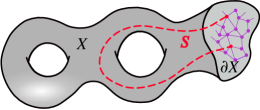
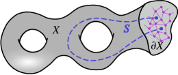
Figure 1. Wilson loop/order operator (left); ’t Hooft loop/disorder operator (right)

Recall from §3.4 that $\mathrsfs{G}^{\vphantom{1*\prime y\vee M}}_{\!G}$ admits two distinguished kinds of loop operators associated to an embedded oriented circle: Wilson and ’t Hooft operators. We also discussed operators on neatly embedded closed intervals $S$, and these carry over to operators in the theory $(\mathrsfs{G}^{\vphantom{1*\prime y\vee M}}_{\!G},\mathrsfs{I})$ on a 3-manifold with latticed boundary. For Wilson operators we require the boundary of $S$ to lie in $\operatorname{Vert}(\Lambda)\subset\Lambda\subset\partial X$. Fix a character $\chi\colon G\to\mathbb{T}$. Then for a principal $G$-bundle $P\to X$ and a section $s\in(\partial P)^{\operatorname{Vert}(\Lambda)}$ over $\operatorname{Vert}(\Lambda)$ we define

(4.25) $$h_{S,\chi}(P,s)=\chi\bigl{(}g(s;S)\bigr{)},$$

where as in (4.17) the group element $g(s,S)\in G$ sends $s(\partial_{-}S)$ to $s(\partial_{+}S)$, after parallel transport along $S$. The partition function with this “Wilson path operator” inserted is

(4.26) $$(\mathrsfs{G}^{\vphantom{1*\prime y\vee M}}_{\!G},\mathrsfs{I})(X,\Lambda)=\sum\limits_{[P]\in\pi_{0}\operatorname{Bun}_{G}(X)}\frac{1}{\#\operatorname{Aut}P}\sum\limits_{s\in(\partial P)^{\operatorname{Vert}(\Lambda)}}h_{S,\chi}(P,s)\prod\limits_{e\in\operatorname{Edge}(\Lambda)}\theta\bigl{(}g(s;e)\bigr{)}.$$

Remark 4.27.

In the language of spin systems $h_{S,\chi}(P,s)$ is called an order operator. It is usually defined for a single vertex of $\Lambda$ rather than a pair of vertices connected by a path (which may be contained in $\partial X$ or can wander into the interior of $X$). Indeed, if we restrict to the untwisted sector in which $P\to X$ is the trivial $G$-bundle then we can define the order operator at a single vertex, but for general $P\to X$ we need the path $S$. We discuss order operators without paths below.

We turn now to the ’t Hooft operator, for which we require the boundary of $S$ to lie in $\partial X\setminus\Lambda$. Fix a conjugacy class $\gamma\subset G$. As in (3.37) we let $\operatorname{Bun}_{G}\bigl{(}X;(S,\gamma)\bigr{)}$ be the groupoid whose objects are principal $G$-bundles $P\to X\setminus S$ with holonomy $\gamma$ about $S$. A bundle $P\to X\setminus S$ is defined on $\Lambda\subset\partial X$, hence $P^{\operatorname{Vert}(\Lambda)}$ is still defined. The partition function with this “’t Hooft path operator” inserted is given by (4.24) with $\operatorname{Bun}_{G}(X)$ replaced by $\operatorname{Bun}_{G}\bigl{(}X;(S,\gamma)\bigr{)}$. In the language of spin systems this is a disorder operator.

There are more general point operators in the boundary theory which do not require the point to lie at the end of a 1-manifold $S$. First, we consider general defects in the topological gauge theory $\mathrsfs{G}^{\vphantom{1*\prime y\vee M}}_{\!G}$ on a closed 2-manifold $Y$. Suppose $y_{1},\dots,y_{N}\in Y$ is a finite set of points. Let $Y^{\prime}$ denote $Y$ with disjoint open disks $D_{y_{\alpha}}$ about the $y_{\alpha}$ removed, and read $Y^{\prime}$ as a bordism with $\partial Y^{\prime}$ incoming. Fix diffeomorphisms $S^{1}\xrightarrow{\;\approx\;}\partial D_{y_{\alpha}}$. Then, as in (3.46), there is a fiber bundle of groupoids

(4.28) $$\pi\colon\operatorname{Bun}_{G}(Y^{\prime})\longrightarrow(G/\!/G)^{\times N}.$$

Fix vector bundles $W_{\alpha}\to G/\!/G$, so $G$-equivariant vector bundles $W_{\alpha}\to G$, and use them as inputs into $\mathrsfs{G}^{\vphantom{1*\prime y\vee M}}_{\!G}(Y^{\prime})$. Then $\mathrsfs{G}^{\vphantom{1*\prime y\vee M}}_{\!G}(Y^{\prime})(W_{1},\dots,W_{N})$ is the vector space of sections of

(4.29) $$\pi^{*}(W_{1}\boxtimes\cdots\boxtimes W_{N})\longrightarrow\operatorname{Bun}_{G}(Y^{\prime}).$$

Observe that because of nontrivial automorphisms of $G$-bundles, this may be the zero vector space.

We now describe point operators in the boundary theory $\mathrsfs{I}=\mathrsfs{I}_{G,\theta}$ on a latticed surface $(Y,\Lambda)$. There are two types of such point defects: order and disorder operators. For an order operator at $y_{i}$ we have $y_{i}\in\operatorname{Vert}(\Lambda)$; the vector bundle $W_{i}\to G/\!/G$ is supported at $e/\!/G$, so is a representation of $G$; and we fix a vector $\xi_{i}\in W_{i}$. (Identify $W_{i}$ with its fiber at $e$.) For a disorder operator at $y_{j}$ we have $y_{j}\in Y\setminus\Lambda$; the vector bundle $W_{j}\to G/\!/G$ has trivial action of centralizers, so is a vector space $W_{j,g/G}$ for each conjugacy class $g/G$; and we fix a vector $\xi_{j,g/G}\in W_{j,g/G}$. An irreducible $W_{j}\to G/\!/G$ is supported on a single conjugacy class; the vector $\xi$ vanishes at other conjugacy classes. Suppose there is order operator data at vertices $v_{1},\dots,v_{L}$ and disorder operator data at faces $f_{1},\dots,f_{M}$. Then the generalization of (4.21) with these point defects is

(4.30) $$\quad\mathrsfs{I}(Y,\Lambda)(W_{1},\dots,W_{L+M})[Q]\\ =\sum\limits_{s\in Q^{\operatorname{Vert}(\Lambda)}}\left\{\bigotimes\limits_{i=1}^{L}\bigl{(}s(v_{i})\times\xi_{i}\bigr{)}\;\otimes\bigotimes\limits_{j=K+1}^{M}\xi_{j,\operatorname{hol}_{j}(Q)}\right\}\prod\limits_{e\in\operatorname{Edge}(\Lambda)}\!\!\theta\bigl{(}g(s;e)\bigr{)}.$$

Here $Q\to Y^{\prime}$ is a $G$-bundle; $\operatorname{hol}_{j}(Q)$ is the holonomy about $f_{j}$, a conjugacy class in $G$; and $s(v_{i})\times\xi_{i}\in Q_{v_{i}}\times^{\vphantom{1*\prime y\vee M}}_{G}W_{i}$ is a vector in the vector space defined by mixing the $G$-torsor $Q_{v_{i}}$ with the $G$-representation $W_{i}$.

4.5. Kramers-Wannier duality as electromagnetic duality

We investigate the effect of electromagnetic duality in finite abelian gauge theory (§3.3) on the Ising boundary theories. The following is stated earlier as Theorem 1.13.

Theorem 4.31.

Electromagnetic duality for 3-dimensional finite abelian gauge theory extends to the Ising boundary conditions of lattice theories, whereon it becomes Kramers-Wannier duality. It interchanges the action $\theta$ with its Fourier transform $\theta^{\vee}$. Order operators of the Ising model are boundary points of Wilson loops, disorder operators boundary points of ’t Hooft loops, and they are interchanged under duality.

The remainder of this section is devoted to an explicit proof on a closed latticed surface. The isomorphism of full boundary lattice theories is proved in a more general context in §8.3.

As a preliminary we state without proof properties of the finite Fourier transform (3.23).

Lemma 4.32.

Let $\phi\colon M\to N$ be a homomorphism of finite abelian groups, $\phi^{\vee}\colon N^{\vee}\to M^{\vee}$ the Pontrjagin dual homomorphism, and $\mathfrak{F}^{\vphantom{1*\prime y\vee M}}_{\!M}\colon\operatorname{Fun}(M)\to\operatorname{Fun}(M^{\vee})$ the Fourier transform.

1. If $f\in\operatorname{Fun}(M)$, then

   (4.33) $$\mathfrak{F}^{\vphantom{1*\prime y\vee M}}_{\!N}(\phi_{*}f)=\sqrt{\frac{\#M}{\#N}}\;(\phi^{\vee})^{*}(\mathfrak{F}^{\vphantom{1*\prime y\vee M}}_{\!M}f).$$

2. If $g\in\operatorname{Fun}(N)$, then

   (4.34) $$\mathfrak{F}^{\vphantom{1*\prime y\vee M}}_{\!M}(\phi^{*}g)=\sqrt{\frac{\#M}{\#N}}\;(\phi^{\vee})_{*}(\mathfrak{F}^{\vphantom{1*\prime y\vee M}}_{\!N}g).$$

3. Let

   (4.35) $$1\longrightarrow\mathbb{T}\xrightarrow{\;\;\lambda\;\;}\widetilde{L}\longrightarrow L\longrightarrow 0$$

   be a central extension and

   (4.36) $$0\longrightarrow L^{\vee}\longrightarrow\widetilde{L}^{\vee}\xrightarrow{\;\;\lambda^{\vee}\;\;}{\mathbb{Z}}\longrightarrow 0$$

   its Pontrjagin dual. Then the Fourier transform $\operatorname{Fun}(\widetilde{L})\to\operatorname{Fun}(\widetilde{L}^{\vee})$ restricts to an isomorphism of the vector space of sections of the line bundle over $L$ associated to (4.35) with functions on the $L^{\vee}$-torsor $(\lambda^{\vee})^{-1}(1)\subset\widetilde{L}^{\vee}$.

Suppose now the homomorphisms

(4.37) $$\begin{gathered}\lx@xy@svg{\hbox{\raise 0.0pt\hbox{\kern 10.55467pt\hbox{\ignorespaces\ignorespaces\ignorespaces\hbox{\vtop{\kern 0.0pt\offinterlineskip\halign{\entry@#!@&&\entry@@#!@\cr&&\crcr}}}\ignorespaces{\hbox{\kern-10.55467pt\raise 0.0pt\hbox{\hbox{\kern 0.0pt\raise 0.0pt\hbox{\hbox{\kern 3.0pt\raise 0.0pt\hbox{$\textstyle{M^{\prime}\;\ignorespaces\ignorespaces\ignorespaces\ignorespaces}$}}}}}}}\ignorespaces\ignorespaces\ignorespaces\ignorespaces{\hbox{\kern 10.55469pt\raise 0.0pt\hbox{\hbox{\kern 0.0pt\raise 0.0pt\hbox{\lx@xy@hook{1}}}}}}{\hbox{\lx@xy@droprule}}\ignorespaces\ignorespaces\ignorespaces{\hbox{\kern 17.26945pt\raise 5.30833pt\hbox{{}\hbox{\kern 0.0pt\raise 0.0pt\hbox{\hbox{\kern 3.0pt\hbox{\hbox{\kern 0.0pt\raise-2.30833pt\hbox{$\scriptstyle{i}$}}}\kern 3.0pt}}}}}}\ignorespaces{\hbox{\kern 34.55467pt\raise 0.0pt\hbox{\hbox{\kern 0.0pt\raise 0.0pt\hbox{\lx@xy@tip{1}\lx@xy@tip{-1}}}}}}{\hbox{\lx@xy@droprule}}{\hbox{\lx@xy@droprule}}{\hbox{\kern 34.55467pt\raise 0.0pt\hbox{\hbox{\kern 0.0pt\raise 0.0pt\hbox{\hbox{\kern 3.0pt\raise 0.0pt\hbox{$\textstyle{M\ignorespaces\ignorespaces\ignorespaces\ignorespaces}$}}}}}}}\ignorespaces\ignorespaces\ignorespaces\ignorespaces{}{\hbox{\lx@xy@droprule}}\ignorespaces\ignorespaces\ignorespaces{\hbox{\kern 54.8878pt\raise 4.50694pt\hbox{{}\hbox{\kern 0.0pt\raise 0.0pt\hbox{\hbox{\kern 3.0pt\hbox{\hbox{\kern 0.0pt\raise-1.50694pt\hbox{$\scriptstyle{\pi}$}}}\kern 3.0pt}}}}}}\ignorespaces{\hbox{\kern 75.34633pt\raise 0.0pt\hbox{\hbox{\kern 0.0pt\raise 0.0pt\hbox{\hbox{\kern-3.0pt\lower 0.0pt\hbox{\lx@xy@tip{1}\lx@xy@tip{-1}}}\lx@xy@tip{1}\lx@xy@tip{-1}}}}}}{\hbox{\lx@xy@droprule}}{\hbox{\lx@xy@droprule}}{\hbox{\kern 75.34633pt\raise 0.0pt\hbox{\hbox{\kern 0.0pt\raise 0.0pt\hbox{\hbox{\kern 3.0pt\raise 0.0pt\hbox{$\textstyle{M^{\prime\prime}}$}}}}}}}\ignorespaces}}}}\ignorespaces\end{gathered} \textstyle{M^{\prime}\;\ignorespaces\ignorespaces\ignorespaces\ignorespaces} \scriptstyle{i} \textstyle{M\ignorespaces\ignorespaces\ignorespaces\ignorespaces} \scriptstyle{\pi} \textstyle{M^{\prime\prime}} \textstyle{M^{\prime}\;\ignorespaces\ignorespaces\ignorespaces\ignorespaces} \scriptstyle{i} \textstyle{M\ignorespaces\ignorespaces\ignorespaces\ignorespaces} \scriptstyle{\pi} \textstyle{M^{\prime\prime}}$$

of finite abelian groups satisfy $\pi\circ i=0$. Let $K=\operatorname{Ker}\pi$ and $H=\operatorname{Ker}\pi/\operatorname{Im}i$. The Pontrjagin dual to (4.37) is

(4.38) $$\begin{gathered}\lx@xy@svg{\hbox{\raise 0.0pt\hbox{\kern 11.03249pt\hbox{\ignorespaces\ignorespaces\ignorespaces\hbox{\vtop{\kern 0.0pt\offinterlineskip\halign{\entry@#!@&&\entry@@#!@\cr&&\crcr}}}\ignorespaces{\hbox{\kern-11.03249pt\raise 0.0pt\hbox{\hbox{\kern 0.0pt\raise 0.0pt\hbox{\hbox{\kern 3.0pt\raise 0.0pt\hbox{$\textstyle{{M^{\prime}}^{\vee}}$}}}}}}}{\hbox{\kern 35.03249pt\raise 0.0pt\hbox{\hbox{\kern 0.0pt\raise 0.0pt\hbox{\hbox{\kern 3.0pt\raise 0.0pt\hbox{$\textstyle{M^{\vee}\ignorespaces\ignorespaces\ignorespaces\ignorespaces}$}}}}}}}\ignorespaces\ignorespaces\ignorespaces\ignorespaces{}{\hbox{\lx@xy@droprule}}\ignorespaces\ignorespaces\ignorespaces{\hbox{\kern 21.63815pt\raise 5.86389pt\hbox{{}\hbox{\kern 0.0pt\raise 0.0pt\hbox{\hbox{\kern 3.0pt\hbox{\hbox{\kern 0.0pt\raise-2.86389pt\hbox{$\scriptstyle{i^{\vee}}$}}}\kern 3.0pt}}}}}}\ignorespaces{\hbox{\kern 11.0325pt\raise 0.0pt\hbox{\hbox{\kern 0.0pt\raise 0.0pt\hbox{\hbox{\kern 3.0pt\lower 0.0pt\hbox{\lx@xy@tip{1}\lx@xy@tip{-1}}}\lx@xy@tip{1}\lx@xy@tip{-1}}}}}}{\hbox{\lx@xy@droprule}}{\hbox{\lx@xy@droprule}}{\hbox{\kern 79.55748pt\raise 0.0pt\hbox{\hbox{\kern 0.0pt\raise 0.0pt\hbox{\hbox{\kern 3.0pt\raise 0.0pt\hbox{$\textstyle{{M^{\prime\prime}}^{\vee}\ignorespaces\ignorespaces\ignorespaces\ignorespaces}$}}}}}}}\ignorespaces\ignorespaces\ignorespaces\ignorespaces{\hbox{\kern 79.55748pt\raise 0.0pt\hbox{\hbox{\kern 0.0pt\raise 0.0pt\hbox{\lx@xy@hook{-1}}}}}}{\hbox{\lx@xy@droprule}}\ignorespaces\ignorespaces\ignorespaces{\hbox{\kern 64.30244pt\raise 5.0625pt\hbox{{}\hbox{\kern 0.0pt\raise 0.0pt\hbox{\hbox{\kern 3.0pt\hbox{\hbox{\kern 0.0pt\raise-2.0625pt\hbox{$\scriptstyle{\pi^{\vee}}$}}}\kern 3.0pt}}}}}}\ignorespaces{\hbox{\kern 55.55748pt\raise 0.0pt\hbox{\hbox{\kern 0.0pt\raise 0.0pt\hbox{\lx@xy@tip{1}\lx@xy@tip{-1}}}}}}{\hbox{\lx@xy@droprule}}{\hbox{\lx@xy@droprule}}\ignorespaces}}}}\ignorespaces\end{gathered} \textstyle{{M^{\prime}}^{\vee}} \textstyle{M^{\vee}\ignorespaces\ignorespaces\ignorespaces\ignorespaces} \scriptstyle{i^{\vee}} \textstyle{{M^{\prime\prime}}^{\vee}\ignorespaces\ignorespaces\ignorespaces\ignorespaces} \scriptstyle{\pi^{\vee}} \textstyle{{M^{\prime}}^{\vee}} \textstyle{M^{\vee}\ignorespaces\ignorespaces\ignorespaces\ignorespaces} \scriptstyle{i^{\vee}} \textstyle{{M^{\prime\prime}}^{\vee}\ignorespaces\ignorespaces\ignorespaces\ignorespaces} \scriptstyle{\pi^{\vee}}$$

Set $\widetilde{K}=\operatorname{Ker}i^{\vee}$ and $\widetilde{H}=\operatorname{Ker}i^{\vee}/\operatorname{Im}\pi^{\vee}$. ($\widetilde{H}$ and $H$ are in Pontrjagin duality.) Consider the diagrams

(4.39) $$\begin{gathered}\lx@xy@svg{\hbox{\raise 0.0pt\hbox{\kern 9.52188pt\hbox{\ignorespaces\ignorespaces\ignorespaces\hbox{\vtop{\kern 0.0pt\offinterlineskip\halign{\entry@#!@&&\entry@@#!@\cr&\\\crcr}}}\ignorespaces{\hbox{\kern-7.60416pt\raise 0.0pt\hbox{\hbox{\kern 0.0pt\raise 0.0pt\hbox{\hbox{\kern 3.0pt\raise 0.0pt\hbox{$\textstyle{K\ignorespaces\ignorespaces\ignorespaces\ignorespaces\ignorespaces\ignorespaces\ignorespaces\ignorespaces}$}}}}}}}\ignorespaces\ignorespaces\ignorespaces\ignorespaces{\hbox{\kern 7.60417pt\raise 0.0pt\hbox{\hbox{\kern 0.0pt\raise 0.0pt\hbox{\lx@xy@hook{1}}}}}}{\hbox{\lx@xy@droprule}}\ignorespaces\ignorespaces\ignorespaces{\hbox{\kern 15.35832pt\raise 5.98889pt\hbox{{}\hbox{\kern 0.0pt\raise 0.0pt\hbox{\hbox{\kern 3.0pt\hbox{\hbox{\kern 0.0pt\raise-1.62779pt\hbox{$\scriptstyle{j}$}}}\kern 3.0pt}}}}}}\ignorespaces{\hbox{\kern 31.60416pt\raise 0.0pt\hbox{\hbox{\kern 0.0pt\raise 0.0pt\hbox{\lx@xy@tip{1}\lx@xy@tip{-1}}}}}}{\hbox{\lx@xy@droprule}}{\hbox{\lx@xy@droprule}}\ignorespaces\ignorespaces\ignorespaces\ignorespaces{}{\hbox{\lx@xy@droprule}}\ignorespaces\ignorespaces\ignorespaces{\hbox{\kern-9.52188pt\raise-15.83804pt\hbox{{}\hbox{\kern 0.0pt\raise 0.0pt\hbox{\hbox{\kern 3.0pt\hbox{\hbox{\kern 0.0pt\raise-0.8264pt\hbox{$\scriptstyle{p}$}}}\kern 3.0pt}}}}}}\ignorespaces{\hbox{\kern 0.0pt\raise-27.0pt\hbox{\hbox{\kern 0.0pt\raise 0.0pt\hbox{\hbox{\kern 0.0pt\lower-3.0pt\hbox{\lx@xy@tip{1}\lx@xy@tip{-1}}}\lx@xy@tip{1}\lx@xy@tip{-1}}}}}}{\hbox{\lx@xy@droprule}}{\hbox{\lx@xy@droprule}}{\hbox{\kern 31.60416pt\raise 0.0pt\hbox{\hbox{\kern 0.0pt\raise 0.0pt\hbox{\hbox{\kern 3.0pt\raise 0.0pt\hbox{$\textstyle{M}$}}}}}}}{\hbox{\kern-7.56248pt\raise-36.83331pt\hbox{\hbox{\kern 0.0pt\raise 0.0pt\hbox{\hbox{\kern 3.0pt\raise 0.0pt\hbox{$\textstyle{H}$}}}}}}}\ignorespaces}}}}\ignorespaces\qquad\qquad\qquad\lx@xy@svg{\hbox{\raise 0.0pt\hbox{\kern 11.55557pt\hbox{\ignorespaces\ignorespaces\ignorespaces\hbox{\vtop{\kern 0.0pt\offinterlineskip\halign{\entry@#!@&&\entry@@#!@\cr&\\\crcr}}}\ignorespaces{\hbox{\kern-5.77779pt\raise 0.0pt\hbox{\hbox{\kern 0.0pt\raise 0.0pt\hbox{\hbox{\kern 3.0pt\raise 0.0pt\hbox{$\textstyle{\widetilde{K}\ignorespaces\ignorespaces\ignorespaces\ignorespaces\ignorespaces\ignorespaces\ignorespaces\ignorespaces}$}}}}}}}\ignorespaces\ignorespaces\ignorespaces\ignorespaces{\hbox{\kern 5.77779pt\raise 0.0pt\hbox{\hbox{\kern 0.0pt\raise 0.0pt\hbox{\lx@xy@hook{1}}}}}}{\hbox{\lx@xy@droprule}}\ignorespaces\ignorespaces\ignorespaces{\hbox{\kern 14.24236pt\raise 6.61111pt\hbox{{}\hbox{\kern 0.0pt\raise 0.0pt\hbox{\hbox{\kern 3.0pt\hbox{\hbox{\kern 0.0pt\raise-3.61111pt\hbox{$\scriptstyle{\tilde{\jmath}}$}}}\kern 3.0pt}}}}}}\ignorespaces{\hbox{\kern 29.77779pt\raise 0.0pt\hbox{\hbox{\kern 0.0pt\raise 0.0pt\hbox{\lx@xy@tip{1}\lx@xy@tip{-1}}}}}}{\hbox{\lx@xy@droprule}}{\hbox{\lx@xy@droprule}}\ignorespaces\ignorespaces\ignorespaces\ignorespaces{}{\hbox{\lx@xy@droprule}}\ignorespaces\ignorespaces\ignorespaces{\hbox{\kern-11.55557pt\raise-15.12198pt\hbox{{}\hbox{\kern 0.0pt\raise 0.0pt\hbox{\hbox{\kern 3.0pt\hbox{\hbox{\kern 0.0pt\raise-3.61111pt\hbox{$\scriptstyle{\tilde{p}}$}}}\kern 3.0pt}}}}}}\ignorespaces{\hbox{\kern 0.0pt\raise-27.58331pt\hbox{\hbox{\kern 0.0pt\raise 0.0pt\hbox{\hbox{\kern 0.0pt\lower-3.0pt\hbox{\lx@xy@tip{1}\lx@xy@tip{-1}}}\lx@xy@tip{1}\lx@xy@tip{-1}}}}}}{\hbox{\lx@xy@droprule}}{\hbox{\lx@xy@droprule}}{\hbox{\kern 29.77779pt\raise 0.0pt\hbox{\hbox{\kern 0.0pt\raise 0.0pt\hbox{\hbox{\kern 3.0pt\raise 0.0pt\hbox{$\textstyle{M^{\vee}}$}}}}}}}{\hbox{\kern-5.77779pt\raise-37.80554pt\hbox{\hbox{\kern 0.0pt\raise 0.0pt\hbox{\hbox{\kern 3.0pt\raise 0.0pt\hbox{$\textstyle{\widetilde{H}}$}}}}}}}\ignorespaces}}}}\ignorespaces\end{gathered} \textstyle{K\ignorespaces\ignorespaces\ignorespaces\ignorespaces\ignorespaces\ignorespaces\ignorespaces\ignorespaces} \scriptstyle{j} \scriptstyle{p} \textstyle{M} \textstyle{H} \textstyle{\widetilde{K}\ignorespaces\ignorespaces\ignorespaces\ignorespaces\ignorespaces\ignorespaces\ignorespaces\ignorespaces} \scriptstyle{\tilde{\jmath}} \scriptstyle{\tilde{p}} \textstyle{M^{\vee}} \textstyle{\widetilde{H}} \textstyle{K\ignorespaces\ignorespaces\ignorespaces\ignorespaces\ignorespaces\ignorespaces\ignorespaces\ignorespaces} \scriptstyle{j} \scriptstyle{p} \textstyle{M} \textstyle{H} \textstyle{\widetilde{K}\ignorespaces\ignorespaces\ignorespaces\ignorespaces\ignorespaces\ignorespaces\ignorespaces\ignorespaces} \scriptstyle{\tilde{\jmath}} \scriptstyle{\tilde{p}} \textstyle{M^{\vee}} \textstyle{\widetilde{H}}$$

and suppose $\Theta\in\operatorname{Fun}(M)$.

Lemma 4.40.

We have the following equality of Fourier transforms:

(4.41) $$\mathfrak{F}_{H}(p_{*}\,j^{*}\Theta)=\frac{\#K}{\sqrt{\#M\cdot\#H}}\;\tilde{p}_{*}\,\tilde{\jmath}^{*}\,\mathfrak{F}_{M}(\Theta).$$

Proof.

Apply Lemma 4.32(i),(ii) and use the pullback square

(4.42) $$\begin{gathered}\lx@xy@svg{\hbox{\raise 0.0pt\hbox{\kern 11.55557pt\hbox{\ignorespaces\ignorespaces\ignorespaces\hbox{\vtop{\kern 0.0pt\offinterlineskip\halign{\entry@#!@&&\entry@@#!@\cr&\\&\crcr}}}\ignorespaces{\hbox{\kern-5.77779pt\raise 0.0pt\hbox{\hbox{\kern 0.0pt\raise 0.0pt\hbox{\hbox{\kern 3.0pt\raise 0.0pt\hbox{$\textstyle{\widetilde{K}\ignorespaces\ignorespaces\ignorespaces\ignorespaces\ignorespaces\ignorespaces\ignorespaces\ignorespaces}$}}}}}}}\ignorespaces\ignorespaces\ignorespaces\ignorespaces{}{\hbox{\lx@xy@droprule}}\ignorespaces\ignorespaces\ignorespaces{\hbox{\kern 20.83687pt\raise 6.61111pt\hbox{{}\hbox{\kern 0.0pt\raise 0.0pt\hbox{\hbox{\kern 3.0pt\hbox{\hbox{\kern 0.0pt\raise-3.61111pt\hbox{$\scriptstyle{\tilde{\jmath}}$}}}\kern 3.0pt}}}}}}\ignorespaces{\hbox{\kern 42.96683pt\raise 0.0pt\hbox{\hbox{\kern 0.0pt\raise 0.0pt\hbox{\lx@xy@tip{1}\lx@xy@tip{-1}}}}}}{\hbox{\lx@xy@droprule}}{\hbox{\lx@xy@droprule}}\ignorespaces\ignorespaces\ignorespaces\ignorespaces{}{\hbox{\lx@xy@droprule}}\ignorespaces\ignorespaces\ignorespaces{\hbox{\kern-11.55557pt\raise-17.83736pt\hbox{{}\hbox{\kern 0.0pt\raise 0.0pt\hbox{\hbox{\kern 3.0pt\hbox{\hbox{\kern 0.0pt\raise-3.61111pt\hbox{$\scriptstyle{\tilde{p}}$}}}\kern 3.0pt}}}}}}\ignorespaces{\hbox{\kern 0.0pt\raise-29.41663pt\hbox{\hbox{\kern 0.0pt\raise 0.0pt\hbox{\lx@xy@tip{1}\lx@xy@tip{-1}}}}}}{\hbox{\lx@xy@droprule}}{\hbox{\lx@xy@droprule}}{\hbox{\kern 42.96683pt\raise 0.0pt\hbox{\hbox{\kern 0.0pt\raise 0.0pt\hbox{\hbox{\kern 3.0pt\raise 0.0pt\hbox{$\textstyle{M^{\vee}\ignorespaces\ignorespaces\ignorespaces\ignorespaces}$}}}}}}}\ignorespaces\ignorespaces\ignorespaces\ignorespaces{}{\hbox{\lx@xy@droprule}}\ignorespaces\ignorespaces\ignorespaces{\hbox{\kern 53.22932pt\raise-17.83736pt\hbox{{}\hbox{\kern 0.0pt\raise 0.0pt\hbox{\hbox{\kern 3.0pt\hbox{\hbox{\kern 0.0pt\raise-2.18335pt\hbox{$\scriptstyle{j^{\vee}}$}}}\kern 3.0pt}}}}}}\ignorespaces{\hbox{\kern 53.22932pt\raise-28.24998pt\hbox{\hbox{\kern 0.0pt\raise 0.0pt\hbox{\lx@xy@tip{1}\lx@xy@tip{-1}}}}}}{\hbox{\lx@xy@droprule}}{\hbox{\lx@xy@droprule}}{\hbox{\kern-5.77779pt\raise-39.63885pt\hbox{\hbox{\kern 0.0pt\raise 0.0pt\hbox{\hbox{\kern 3.0pt\raise 0.0pt\hbox{$\textstyle{\widetilde{H}\ignorespaces\ignorespaces\ignorespaces\ignorespaces}$}}}}}}}\ignorespaces\ignorespaces\ignorespaces\ignorespaces{}{\hbox{\lx@xy@droprule}}\ignorespaces\ignorespaces\ignorespaces{\hbox{\kern 13.60031pt\raise-33.8958pt\hbox{{}\hbox{\kern 0.0pt\raise 0.0pt\hbox{\hbox{\kern 3.0pt\hbox{\hbox{\kern 0.0pt\raise-1.38196pt\hbox{$\scriptstyle{p^{\vee}}$}}}\kern 3.0pt}}}}}}\ignorespaces{\hbox{\kern 29.77779pt\raise-39.63885pt\hbox{\hbox{\kern 0.0pt\raise 0.0pt\hbox{\lx@xy@tip{1}\lx@xy@tip{-1}}}}}}{\hbox{\lx@xy@droprule}}{\hbox{\lx@xy@droprule}}{\hbox{\kern 29.77779pt\raise-39.63885pt\hbox{\hbox{\kern 0.0pt\raise 0.0pt\hbox{\hbox{\kern 3.0pt\raise 0.0pt\hbox{$\textstyle{M^{\vee}/\operatorname{Im}\pi^{\vee}}$}}}}}}}\ignorespaces}}}}\ignorespaces\end{gathered} \textstyle{\widetilde{K}\ignorespaces\ignorespaces\ignorespaces\ignorespaces\ignorespaces\ignorespaces\ignorespaces\ignorespaces} \scriptstyle{\tilde{\jmath}} \scriptstyle{\tilde{p}} \textstyle{M^{\vee}\ignorespaces\ignorespaces\ignorespaces\ignorespaces} \scriptstyle{j^{\vee}} \textstyle{\widetilde{H}\ignorespaces\ignorespaces\ignorespaces\ignorespaces} \scriptstyle{p^{\vee}} \textstyle{M^{\vee}/\operatorname{Im}\pi^{\vee}} \textstyle{\widetilde{K}\ignorespaces\ignorespaces\ignorespaces\ignorespaces\ignorespaces\ignorespaces\ignorespaces\ignorespaces} \scriptstyle{\tilde{\jmath}} \scriptstyle{\tilde{p}} \textstyle{M^{\vee}\ignorespaces\ignorespaces\ignorespaces\ignorespaces} \scriptstyle{j^{\vee}} \textstyle{\widetilde{H}\ignorespaces\ignorespaces\ignorespaces\ignorespaces} \scriptstyle{p^{\vee}} \textstyle{M^{\vee}/\operatorname{Im}\pi^{\vee}}$$

∎

Fix $\eta\in M^{\prime\prime}$ and $\omega\in{M^{\prime}}^{\vee}$. Then the $K$-torsor $K_{\eta}=\pi^{-1}(\eta)$ and $\widetilde{K}$-torsor $\widetilde{K}_{\omega}=(i^{\vee})^{-1}(\omega)$ fit into the diagrams

(4.43) $$\begin{gathered}\lx@xy@svg{\hbox{\raise 0.0pt\hbox{\kern 9.52188pt\hbox{\ignorespaces\ignorespaces\ignorespaces\hbox{\vtop{\kern 0.0pt\offinterlineskip\halign{\entry@#!@&&\entry@@#!@\cr&\\\crcr}}}\ignorespaces{\hbox{\kern-8.99445pt\raise 0.0pt\hbox{\hbox{\kern 0.0pt\raise 0.0pt\hbox{\hbox{\kern 3.0pt\raise 0.0pt\hbox{$\textstyle{K_{\eta}\ignorespaces\ignorespaces\ignorespaces\ignorespaces\ignorespaces\ignorespaces\ignorespaces\ignorespaces}$}}}}}}}\ignorespaces\ignorespaces\ignorespaces\ignorespaces{\hbox{\kern 8.99445pt\raise 0.0pt\hbox{\hbox{\kern 0.0pt\raise 0.0pt\hbox{\lx@xy@hook{1}}}}}}{\hbox{\lx@xy@droprule}}\ignorespaces\ignorespaces\ignorespaces{\hbox{\kern 15.06041pt\raise 6.12778pt\hbox{{}\hbox{\kern 0.0pt\raise 0.0pt\hbox{\hbox{\kern 3.0pt\hbox{\hbox{\kern 0.0pt\raise-1.48889pt\hbox{$\scriptstyle{j_{\eta}}$}}}\kern 3.0pt}}}}}}\ignorespaces{\hbox{\kern 32.99445pt\raise 0.0pt\hbox{\hbox{\kern 0.0pt\raise 0.0pt\hbox{\lx@xy@tip{1}\lx@xy@tip{-1}}}}}}{\hbox{\lx@xy@droprule}}{\hbox{\lx@xy@droprule}}\ignorespaces\ignorespaces\ignorespaces\ignorespaces{}{\hbox{\lx@xy@droprule}}\ignorespaces\ignorespaces\ignorespaces{\hbox{\kern-9.52188pt\raise-16.82463pt\hbox{{}\hbox{\kern 0.0pt\raise 0.0pt\hbox{\hbox{\kern 3.0pt\hbox{\hbox{\kern 0.0pt\raise-0.8264pt\hbox{$\scriptstyle{p}$}}}\kern 3.0pt}}}}}}\ignorespaces{\hbox{\kern 0.0pt\raise-29.29443pt\hbox{\hbox{\kern 0.0pt\raise 0.0pt\hbox{\hbox{\kern 0.0pt\lower-3.0pt\hbox{\lx@xy@tip{1}\lx@xy@tip{-1}}}\lx@xy@tip{1}\lx@xy@tip{-1}}}}}}{\hbox{\lx@xy@droprule}}{\hbox{\lx@xy@droprule}}{\hbox{\kern 32.99445pt\raise 0.0pt\hbox{\hbox{\kern 0.0pt\raise 0.0pt\hbox{\hbox{\kern 3.0pt\raise 0.0pt\hbox{$\textstyle{M}$}}}}}}}{\hbox{\kern-8.95276pt\raise-39.12775pt\hbox{\hbox{\kern 0.0pt\raise 0.0pt\hbox{\hbox{\kern 3.0pt\raise 0.0pt\hbox{$\textstyle{H_{\eta}}$}}}}}}}\ignorespaces}}}}\ignorespaces\qquad\qquad\qquad\lx@xy@svg{\hbox{\raise 0.0pt\hbox{\kern 11.55557pt\hbox{\ignorespaces\ignorespaces\ignorespaces\hbox{\vtop{\kern 0.0pt\offinterlineskip\halign{\entry@#!@&&\entry@@#!@\cr&\\\crcr}}}\ignorespaces{\hbox{\kern-7.52066pt\raise 0.0pt\hbox{\hbox{\kern 0.0pt\raise 0.0pt\hbox{\hbox{\kern 3.0pt\raise 0.0pt\hbox{$\textstyle{\widetilde{K}_{\omega}\ignorespaces\ignorespaces\ignorespaces\ignorespaces\ignorespaces\ignorespaces\ignorespaces\ignorespaces}$}}}}}}}\ignorespaces\ignorespaces\ignorespaces\ignorespaces{\hbox{\kern 7.52066pt\raise 0.0pt\hbox{\hbox{\kern 0.0pt\raise 0.0pt\hbox{\lx@xy@hook{1}}}}}}{\hbox{\lx@xy@droprule}}\ignorespaces\ignorespaces\ignorespaces{\hbox{\kern 13.86888pt\raise 7.04167pt\hbox{{}\hbox{\kern 0.0pt\raise 0.0pt\hbox{\hbox{\kern 3.0pt\hbox{\hbox{\kern 0.0pt\raise-3.18056pt\hbox{$\scriptstyle{\tilde{\jmath}_{\omega}}$}}}\kern 3.0pt}}}}}}\ignorespaces{\hbox{\kern 31.52066pt\raise 0.0pt\hbox{\hbox{\kern 0.0pt\raise 0.0pt\hbox{\lx@xy@tip{1}\lx@xy@tip{-1}}}}}}{\hbox{\lx@xy@droprule}}{\hbox{\lx@xy@droprule}}\ignorespaces\ignorespaces\ignorespaces\ignorespaces{}{\hbox{\lx@xy@droprule}}\ignorespaces\ignorespaces\ignorespaces{\hbox{\kern-11.55557pt\raise-15.60419pt\hbox{{}\hbox{\kern 0.0pt\raise 0.0pt\hbox{\hbox{\kern 3.0pt\hbox{\hbox{\kern 0.0pt\raise-3.61111pt\hbox{$\scriptstyle{\tilde{p}}$}}}\kern 3.0pt}}}}}}\ignorespaces{\hbox{\kern 0.0pt\raise-28.78886pt\hbox{\hbox{\kern 0.0pt\raise 0.0pt\hbox{\hbox{\kern 0.0pt\lower-3.0pt\hbox{\lx@xy@tip{1}\lx@xy@tip{-1}}}\lx@xy@tip{1}\lx@xy@tip{-1}}}}}}{\hbox{\lx@xy@droprule}}{\hbox{\lx@xy@droprule}}{\hbox{\kern 31.52066pt\raise 0.0pt\hbox{\hbox{\kern 0.0pt\raise 0.0pt\hbox{\hbox{\kern 3.0pt\raise 0.0pt\hbox{$\textstyle{M^{\vee}}$}}}}}}}{\hbox{\kern-7.52066pt\raise-39.0111pt\hbox{\hbox{\kern 0.0pt\raise 0.0pt\hbox{\hbox{\kern 3.0pt\raise 0.0pt\hbox{$\textstyle{\widetilde{H}_{\omega}}$}}}}}}}\ignorespaces}}}}\ignorespaces\end{gathered} \textstyle{K_{\eta}\ignorespaces\ignorespaces\ignorespaces\ignorespaces\ignorespaces\ignorespaces\ignorespaces\ignorespaces} \scriptstyle{j_{\eta}} \scriptstyle{p} \textstyle{M} \textstyle{H_{\eta}} \textstyle{\widetilde{K}_{\omega}\ignorespaces\ignorespaces\ignorespaces\ignorespaces\ignorespaces\ignorespaces\ignorespaces\ignorespaces} \scriptstyle{\tilde{\jmath}_{\omega}} \scriptstyle{\tilde{p}} \textstyle{M^{\vee}} \textstyle{\widetilde{H}_{\omega}} \textstyle{K_{\eta}\ignorespaces\ignorespaces\ignorespaces\ignorespaces\ignorespaces\ignorespaces\ignorespaces\ignorespaces} \scriptstyle{j_{\eta}} \scriptstyle{p} \textstyle{M} \textstyle{H_{\eta}} \textstyle{\widetilde{K}_{\omega}\ignorespaces\ignorespaces\ignorespaces\ignorespaces\ignorespaces\ignorespaces\ignorespaces\ignorespaces} \scriptstyle{\tilde{\jmath}_{\omega}} \scriptstyle{\tilde{p}} \textstyle{M^{\vee}} \textstyle{\widetilde{H}_{\omega}}$$

for the $H$-torsor $H_{\eta}=K_{\eta}/\operatorname{Im}i$ and $\widetilde{H}$-torsor $\widetilde{H}_{\omega}=\widetilde{K}_{\omega}/\operatorname{Im}\pi^{\vee}$. Use the character $\omega\colon M^{\prime}\to{\mathbb{C}}$ to define twisted descent $p^{\omega}_{*}\colon\operatorname{Fun}(K_{\eta})\to\operatorname{Fun}_{\omega}(H_{\eta})$ from $\operatorname{Fun}(K_{\eta})$y to the vector space

(4.44) $$p^{*}\!\operatorname{Fun}_{\omega}(H_{\eta})=\left\{g\colon K_{\eta}\to{\mathbb{C}}:g\bigl{(}k+i(m^{\prime})\bigr{)}=\omega(m^{\prime})^{-1}g(k)\textnormal{ for all $m^{\prime}\in M^{\prime}$}\right\}$$

of sections of the line bundle over $H_{\eta}$ determined by $\omega$: the value of $p_{*}^{\omega}$ on $f\in\operatorname{Fun}(K_{\eta})$ is determined by the formula

(4.45) $$p^{*}p^{\omega}_{*}f(k)=\sum\limits_{m^{\prime}\in M^{\prime}}\omega(m^{\prime})f\bigl{(}k+i(m^{\prime})\bigr{)},\qquad k\in K_{\eta}.$$

There is a similar map $\tilde{p}_{*}^{\eta}$ which interchanges the roles of $\eta$ and $\omega$. Lemma 4.32(iii) tells that the Fourier transform $\mathfrak{F}_{M}$ maps the subspace $(j_{\eta})_{*}p^{*}\operatorname{Fun}_{\omega}(H_{\eta})$ of $\operatorname{Fun}(M)$ to the corresponding subspace $(\tilde{\jmath}_{\omega})_{*}\tilde{p}^{*}\operatorname{Fun}_{\eta}(\widetilde{H}_{\omega})$ of $\operatorname{Fun}(M^{\vee})$. There is no Fourier transform defined a priori on $\operatorname{Fun}_{\omega}(H_{\eta})$, so we define it in terms of $\mathfrak{F}_{M}$, inserting the appropriate factors in Lemma 4.40, and conclude

(4.46) $$\mathfrak{F}_{H_{\eta}}(p_{*}^{\omega}\,j^{*}_{\eta}\Theta)=\frac{\#K}{\sqrt{\#M\cdot\#H}}\;\tilde{p}_{*}^{\eta}\,\tilde{\jmath}^{*}_{\omega}\,\mathfrak{F}_{M}(\Theta).$$

Let $(Y,\Lambda)$ be a closed latticed surface. Let $A$ be a finite abelian group. As in (4.30) we fix data for order and disorder operators, which we take to be irreducible:

(4.47) $$v_{1},\dots,v_{L} \in\operatorname{Vert}(\Lambda),\qquad \omega_{1},\dots,\omega_{L}\in A^{\vee};$$

$$f_{1},\dots,f_{M} \in Y\setminus\Lambda,\qquad \eta_{1},\dots,\eta_{M}\in A.$$

Let $\Lambda^{\vee}$ be a dual lattice (Definition 4.12), chosen so that $f_{1},\dots,f_{M}$ are vertices of $\Lambda^{\vee}$. The cochain complexes

(4.48) $$\begin{gathered}\lx@xy@svg{\hbox{\raise 0.0pt\hbox{\kern 25.39792pt\hbox{\ignorespaces\ignorespaces\ignorespaces\hbox{\vtop{\kern 0.0pt\offinterlineskip\halign{\entry@#!@&&\entry@@#!@\cr&&\\&&\crcr}}}\ignorespaces{\hbox{\kern-21.66458pt\raise 0.0pt\hbox{\hbox{\kern 0.0pt\raise 0.0pt\hbox{\hbox{\kern 3.0pt\raise 0.0pt\hbox{$\textstyle{C^{0}(\Lambda;A)\ignorespaces\ignorespaces\ignorespaces\ignorespaces}$}}}}}}}\ignorespaces\ignorespaces\ignorespaces\ignorespaces{}{\hbox{\lx@xy@droprule}}\ignorespaces\ignorespaces\ignorespaces{\hbox{\kern 31.57622pt\raise 6.075pt\hbox{{}\hbox{\kern 0.0pt\raise 0.0pt\hbox{\hbox{\kern 3.0pt\hbox{\hbox{\kern 0.0pt\raise-3.075pt\hbox{$\scriptstyle{d^{0}}$}}}\kern 3.0pt}}}}}}\ignorespaces{\hbox{\kern 53.13126pt\raise 0.0pt\hbox{\hbox{\kern 0.0pt\raise 0.0pt\hbox{\lx@xy@tip{1}\lx@xy@tip{-1}}}}}}{\hbox{\lx@xy@droprule}}{\hbox{\lx@xy@droprule}}{\hbox{\kern 53.13126pt\raise 0.0pt\hbox{\hbox{\kern 0.0pt\raise 0.0pt\hbox{\hbox{\kern 3.0pt\raise 0.0pt\hbox{$\textstyle{C^{1}(\Lambda;A)\ignorespaces\ignorespaces\ignorespaces\ignorespaces}$}}}}}}}\ignorespaces\ignorespaces\ignorespaces\ignorespaces{}{\hbox{\lx@xy@droprule}}\ignorespaces\ignorespaces\ignorespaces{\hbox{\kern 106.37206pt\raise 6.075pt\hbox{{}\hbox{\kern 0.0pt\raise 0.0pt\hbox{\hbox{\kern 3.0pt\hbox{\hbox{\kern 0.0pt\raise-3.075pt\hbox{$\scriptstyle{d^{1}}$}}}\kern 3.0pt}}}}}}\ignorespaces{\hbox{\kern 127.9271pt\raise 0.0pt\hbox{\hbox{\kern 0.0pt\raise 0.0pt\hbox{\lx@xy@tip{1}\lx@xy@tip{-1}}}}}}{\hbox{\lx@xy@droprule}}{\hbox{\lx@xy@droprule}}{\hbox{\kern 127.9271pt\raise 0.0pt\hbox{\hbox{\kern 0.0pt\raise 0.0pt\hbox{\hbox{\kern 3.0pt\raise 0.0pt\hbox{$\textstyle{C^{2}(\Lambda;A)}$}}}}}}}{\hbox{\kern-25.39792pt\raise-28.13771pt\hbox{\hbox{\kern 0.0pt\raise 0.0pt\hbox{\hbox{\kern 3.0pt\raise 0.0pt\hbox{$\textstyle{C^{2}(\Lambda^{\vee};A^{\vee})}$}}}}}}}{\hbox{\kern 49.39792pt\raise-28.13771pt\hbox{\hbox{\kern 0.0pt\raise 0.0pt\hbox{\hbox{\kern 3.0pt\raise 0.0pt\hbox{$\textstyle{C^{1}(\Lambda^{\vee};A^{\vee})\ignorespaces\ignorespaces\ignorespaces\ignorespaces}$}}}}}}}\ignorespaces\ignorespaces\ignorespaces\ignorespaces{}{\hbox{\lx@xy@droprule}}\ignorespaces\ignorespaces\ignorespaces{\hbox{\kern 35.27979pt\raise-22.06271pt\hbox{{}\hbox{\kern 0.0pt\raise 0.0pt\hbox{\hbox{\kern 3.0pt\hbox{\hbox{\kern 0.0pt\raise-3.075pt\hbox{$\scriptstyle{\partial^{1}}$}}}\kern 3.0pt}}}}}}\ignorespaces{\hbox{\kern 25.39792pt\raise-28.13771pt\hbox{\hbox{\kern 0.0pt\raise 0.0pt\hbox{\lx@xy@tip{1}\lx@xy@tip{-1}}}}}}{\hbox{\lx@xy@droprule}}{\hbox{\lx@xy@droprule}}{\hbox{\kern 124.19376pt\raise-28.13771pt\hbox{\hbox{\kern 0.0pt\raise 0.0pt\hbox{\hbox{\kern 3.0pt\raise 0.0pt\hbox{$\textstyle{C^{0}(\Lambda^{\vee};A^{\vee})\ignorespaces\ignorespaces\ignorespaces\ignorespaces}$}}}}}}}\ignorespaces\ignorespaces\ignorespaces\ignorespaces{}{\hbox{\lx@xy@droprule}}\ignorespaces\ignorespaces\ignorespaces{\hbox{\kern 110.07562pt\raise-22.06271pt\hbox{{}\hbox{\kern 0.0pt\raise 0.0pt\hbox{\hbox{\kern 3.0pt\hbox{\hbox{\kern 0.0pt\raise-3.075pt\hbox{$\scriptstyle{\partial^{0}}$}}}\kern 3.0pt}}}}}}\ignorespaces{\hbox{\kern 100.19376pt\raise-28.13771pt\hbox{\hbox{\kern 0.0pt\raise 0.0pt\hbox{\lx@xy@tip{1}\lx@xy@tip{-1}}}}}}{\hbox{\lx@xy@droprule}}{\hbox{\lx@xy@droprule}}\ignorespaces}}}}\ignorespaces\end{gathered} \textstyle{C^{0}(\Lambda;A)\ignorespaces\ignorespaces\ignorespaces\ignorespaces} \scriptstyle{d^{0}} \textstyle{C^{1}(\Lambda;A)\ignorespaces\ignorespaces\ignorespaces\ignorespaces} \scriptstyle{d^{1}} \textstyle{C^{2}(\Lambda;A)} \textstyle{C^{2}(\Lambda^{\vee};A^{\vee})} \textstyle{C^{1}(\Lambda^{\vee};A^{\vee})\ignorespaces\ignorespaces\ignorespaces\ignorespaces} \scriptstyle{\partial^{1}} \textstyle{C^{0}(\Lambda^{\vee};A^{\vee})\ignorespaces\ignorespaces\ignorespaces\ignorespaces} \scriptstyle{\partial^{0}} \textstyle{C^{0}(\Lambda;A)\ignorespaces\ignorespaces\ignorespaces\ignorespaces} \scriptstyle{d^{0}} \textstyle{C^{1}(\Lambda;A)\ignorespaces\ignorespaces\ignorespaces\ignorespaces} \scriptstyle{d^{1}} \textstyle{C^{2}(\Lambda;A)} \textstyle{C^{2}(\Lambda^{\vee};A^{\vee})} \textstyle{C^{1}(\Lambda^{\vee};A^{\vee})\ignorespaces\ignorespaces\ignorespaces\ignorespaces} \scriptstyle{\partial^{1}} \textstyle{C^{0}(\Lambda^{\vee};A^{\vee})\ignorespaces\ignorespaces\ignorespaces\ignorespaces} \scriptstyle{\partial^{0}}$$

are Pontrjagin dual. The order data determines a character $\omega\colon C^{0}(\Lambda;A)\to{\mathbb{C}}$ and the disorder data an element $\eta\in C^{2}(\Lambda;A)$.

The stack $\operatorname{Bun}_{A}(\Lambda)$ has a small model, the action groupoid of $C^{0}(\Lambda;A)$ acting on $C^{1}(\Lambda;A)$ by translation via $d^{0}$. (An element of $C^{1}(\Lambda;A)$ defines $Q\to\Lambda$ trivialized over $\operatorname{Vert}(\Lambda)$.) The disorder operator acts by restriction to the subgroupoid  $C^{0}(\Lambda;A)$ acting on the $Z^{1}(\Lambda;A)$-torsor $(d^{1})^{-1}(\delta_{\eta})$, where as usual $Z^{1}(\Lambda;A)=\ker d^{1}$. Fix an admissible $\theta\in\operatorname{Fun}(A)$ and let $\Theta\in\operatorname{Fun}\bigl{(}C^{1}(\Lambda;A)\bigr{)}$ be

(4.49) $$\Theta(c)=\prod\limits_{e\in\operatorname{Edge}(\Lambda)}\theta\bigl{(}c(e)\bigr{)},\qquad c\in C^{1}(\Lambda;A).$$

Then the Ising partition function (4.30) is

(4.50) $$\mathrsfs{I}(Y,\Lambda)(z)=\sum\limits_{s\in C^{0}(\Lambda;A)}\omega(s)\cdot\Theta(z+d^{0}s),\qquad z\in(d^{1})^{-1}(\delta_{\eta}).$$

We apply Lemma 4.40 to compute its Fourier transform. Take $M=C^{1}(\Lambda;A)$, $M^{\prime}=B^{1}(\Lambda;A)$, and $M^{\prime\prime}=B^{2}(\Lambda;A)$, where as usual $B^{\bullet}$ denotes the subgroup of boundaries. Then $K=Z^{1}(\Lambda;A)$ and $H=H^{1}(Y;A)\cong\pi_{0}\operatorname{Bun}_{A}(Y)$. First, suppose $\eta=0$ and $\omega=0$: no order or disorder operators. Then (4.50) reduces to $\mathrsfs{I}(Y,\Lambda)=\#H^{0}(Y;A)\cdot p_{*}\,j^{*}\,\Theta$ and (4.41) immediately implies the following, which is part of Theorem 4.31.

Proposition 4.51.

The Fourier transform $\operatorname{Fun}\bigl{(}\pi_{0}\operatorname{Bun}_{A}(Y)\bigr{)}\to\operatorname{Fun}\bigl{(}\pi_{0}\operatorname{Bun}_{A^{\vee}}(Y)\bigr{)}$ maps the Ising partition function $\mathrsfs{I}_{(A,\theta)}(Y,\Lambda)$ to the numerical factor

(4.52) $$\frac{\#Z^{1}(\Lambda;A)}{\sqrt{\#C^{1}(\Lambda;A)\cdot\#H^{1}(Y;A)}}$$

times the Ising partition function $\mathrsfs{I}_{(A^{\vee},\theta^{\vee})}(Y,\Lambda^{\vee})$.

Remark 4.53.

The numerical factor (4.52) equals

(4.54) $$\sqrt{\frac{\#C^{0}(\Lambda;A)}{\#C^{2}(\Lambda;A)}}.$$

Hence if we divide $\mathrsfs{I}_{(A,\theta)}(Y,\Lambda)$ by $\sqrt{\#C^{0}(\Lambda;A)}$, which is a factor of $(\#A)^{-1/2}$ for each vertex, then we achieve precise agreement under Fourier transform. (The extra factor is a special case of a generalized Ising action; see Definition 8.3.)

If there are order and disorder operators, described by $\eta$ and $\omega$, then the Ising partition function (4.50) is $\mathrsfs{I}(Y,\Lambda)=\#H^{0}(Y;A)\cdot p_{*}^{\omega}\,j^{*}_{\eta}\,\Theta$; see  (4.43) and (4.45) for notation. Therefore, (4.46)  tells the equality with the Ising partition function of the dual model, with order and disorder operators exchanged.

Remark 4.55.

We do not prove that electromagnetic duality induces the Fourier transform defined in (4.46). Rather, we complete the proof of Theorem 4.31 in §8.3 in a more general setting.

5. Low energy effective topological field theories

In this section we consider qualitative aspects of the lattice theories. Our discussion is heuristic and conjectural.

To begin, we recall some general principles about quantum systems. First, the low energy behavior of a quantum system is thought to be well-approximated by a scale-independent relativistic quantum field theory. In particular, this is applied to lattice systems, in which case the emergent relativistic invariance is a strong assumption. Furthermore, there is a notion of a gapped quantum system: the Hamiltonian has a spectral gap above the lowest energy. For lattice systems one assumes that this energy gap is bounded below independent of the lattice. Then for a gapped theory, in many cases, the low energy effective field theory is thought to be topological. If we consider a moduli stack $\mathscr{M}$ of quantum theories with fixed discrete parameters, then there is a locus $\Delta\subset\mathscr{M}$ of phase transitions. Points in $\mathscr{M}\setminus\Delta$ may represent gapped or ungapped systems; the points in $\Delta$ labeling first-order phase transitions may also represent gapped systems whereas those points in $\Delta$ labeling higher-order phase transitions represent gapless systems. Path components of $(\mathscr{M}\setminus\Delta)_{\textnormal{gapped}}$ are called gapped phases. Furthermore, the low energy effective field theory associated to a point of $(\mathscr{M}\setminus\Delta)_{\textnormal{gapped}}$ is thought to be a complete invariant of the gapped phase. In this section we use the full force of the global symmetry—the presentation of lattice theories as boundary theories for fully extended finite gauge theory—to deduce constraints on the low energy field theory.

Remark 5.1.

There is also dynamics, the renormalization group flow on $(\mathscr{M}_{G}\setminus\Delta_{G})_{\textnormal{gapped}}$. Its limit points should be the possible low energy theories.

Remark 5.2.

For a fixed finite group $G$ we take $\mathscr{M}_{G}$ as the space of admissible functions on $G$ divided by positive multiplicative rescaling; see §4.1. Since our lattice theories are a limited class of nearest neighbor interactions (see (4.17)), we do not expect a naive renormalization group flow on $\mathscr{M}_{G}$. To construct a flow we would have to project from a chimerical moduli space of all lattice theories with symmetry $G$ back onto this space.

Fix a finite group $G$ and an admissible function $\theta$. Recall the definition of the Hamiltonian in a lattice model from Remark 4.22. There is a Hamiltonian associated to every latticed 1-manifold $(S,\Pi)$ equipped with a principal $G$-bundle $R\to S$. Choose $S=S^{1}$ the standard circle and so $\Pi$ a polygon. The construction (Definition 4.18) of the lattice model applied to the cylinder $[0,1]\times S^{1}$ with embedded “prism” $[0,1]\times\Pi$ defines an endomorphism of the state space of functions on configurations on $\Pi$. This is the Wick-rotated propagation through a unit of time, so is $\exp(-H_{(\Pi,R)})$ for the Hamiltonian operator $H_{(\Pi,R)}$. For the trivial $G$-bundle $S^{1}\times G\to S^{1}$ the operator $H_{\Pi,R}$ is the usual Hamiltonian, but there are twisted sectors and so “twisted Hamiltonians” for nontrivial $R\to S^{1}$. Full locality permits us to relate different sectors, at least in principle, by modifying $R\to S^{1}$ over small intervals in $S^{1}$. Recall that $\theta\colon G\to{\mathbb{R}}$ achieves its maximum at the identity element $e\in G$. Assume that $e$ is the unique maximum point of $\theta$. It follows that in the untwisted sector the constant $G$-valued function on vertices of $\Pi$ is a minimal energy configuration. Furthermore, the minimal energy configuration in a twisted sector has energy dependent on values of $\theta$ on $G\setminus\{e\}$, so has strictly larger energy than the minimal energy in the untwisted sector. That difference may or may not be bounded away from zero as we vary $\Pi$.

Remark 5.3.

The strong assumption that the low energy effective field theory be fully local implies that ‘low energy’ must also be fully local in the following sense. ‘Low’ is a global minimum—the minimal energy in the untwisted sector—and so if a twisted sector has minimal energy uniformly larger than the global minimum, its states are not present in the low energy approximating field theory: the field theory has value the zero vector space in that sector.

Let $\mathscr{M}_{G}$ denote the space of admissible functions on $G$, up to rescaling. As above, we assume a locus $\Delta_{G}\subset\mathscr{M}_{G}$ of lattice systems at which phase transitions occur, and we restrict to the subset of the complement representing gapped theories. Then associated to $\theta\in(\mathscr{M}_{G}\setminus\Delta_{G})_{\textnormal{gapped}}$ we expect an effective low energy topological field theory. Since the lattice model $\mathrsfs{I}_{(G,\theta)}$ has a global symmetry group $G$, encoded in strong form by realizing $\mathrsfs{I}_{(G,\theta)}$ as the boundary theory of 3-dimensional pure gauge theory $\mathrsfs{G}^{\vphantom{1*\prime y\vee M}}_{\!G}$, we expect the same for its low energy approximation $\mathrsfs{L}_{(G,\theta)}$. Now we are on solid mathematical ground: $\mathrsfs{L}_{(G,\theta)}$  is a topological boundary theory for an extended topological field theory. In §3.5 we described how a subgroup $H\subset G$ gives rise to a topological boundary theory $\mathrsfs{B}^{\vphantom{1*\prime y\vee M}}_{\!H}$, and in Remark 3.51 we quoted a (straightforward) theorem [EGNO, Corollary 7.12.20] in the theory of tensor categories to the effect that every topological boundary theory which is indecomposable is built in this way from a subgroup $H\subset G$ and a central extension of $H$. We also argued in Remark 3.51 that we do not expect to see nontrivial central extensions. Furthermore, the topological theory corresponding to $H$ (no central extension) is realized as $\mathrsfs{I}_{(G,\theta_{H})}$ for $\theta_{H}\in\mathscr{M}_{G}$ the extreme point at which $\theta_{H}$ is the characteristic function of $H$; see Remark 4.23. Given these facts, it seems reasonable to propose that neither nontrivial central extensions nor decomposable boundary theories occur.

Conjecture 5.4.

The low energy field theory $\mathrsfs{L}_{(G,\theta)}$, $\theta\in(\mathscr{M}_{G}\setminus\Delta_{G})_{\textnormal{gapped}}$, is $\mathrsfs{B}^{\vphantom{1*\prime y\vee M}}_{\!H}$ for some subgroup $H\subset G$.

Remark 5.5.

As explained in §3.5 the boundary theory $\mathrsfs{B}^{\vphantom{1*\prime y\vee M}}_{\!H}$ implements symmetry breaking from $G$ to $H$. Therefore, Conjecture 5.4 asserts that gapped phases of Ising lattice models are distinguished by symmetry breaking, which realizes Landau’s vision for this class of models.

Remark 5.6.

Conjecture 5.4 predicts that the renormalization group flow (Remark 5.1) has limit points $\theta_{H}\in\mathscr{M}_{G}$ corresponding to subgroups $H\subset G$.

In the remainder of this section we describe explicitly the special case of the classical Ising model $G=\mbox{$\raisebox{-0.70007pt}{\rotatebox{9.0}{\tiny/}}\mu\raisebox{-4.2194pt}{\scalebox{2.0}{$\color[rgb]{1,1,1}.$}}\raisebox{3.7889pt}{$\color[rgb]{1,1,1}.$}\hskip 4.60007pt$}_{2}$. An admissible function $\theta\colon\mbox{$\raisebox{-0.70007pt}{\rotatebox{9.0}{\tiny/}}\mu\raisebox{-4.2194pt}{\scalebox{2.0}{$\color[rgb]{1,1,1}.$}}\raisebox{3.7889pt}{$\color[rgb]{1,1,1}.$}\hskip 4.60007pt$}_{2}\to{\mathbb{R}}$ can be normalized so $\theta(1)=1$; then $\theta(-1)=a$ with $0\leq a\leq 1$. Thus $\mathscr{M}_{\mbox{$\raisebox{-0.49005pt}{\rotatebox{9.0}{\tiny/}}\mu\raisebox{-2.95358pt}{\scalebox{2.0}{$\color[rgb]{1,1,1}.$}}\raisebox{2.65222pt}{$\color[rgb]{1,1,1}.$}\hskip 3.22005pt$}_{2}}\cong[0,1]$. The extreme point $a=0$ corresponds to the trivial subgroup $1\subset\mbox{$\raisebox{-0.70007pt}{\rotatebox{9.0}{\tiny/}}\mu\raisebox{-4.2194pt}{\scalebox{2.0}{$\color[rgb]{1,1,1}.$}}\raisebox{3.7889pt}{$\color[rgb]{1,1,1}.$}\hskip 4.60007pt$}_{2}$; the extreme point $a=1$ to the full subgroup $\mbox{$\raisebox{-0.70007pt}{\rotatebox{9.0}{\tiny/}}\mu\raisebox{-4.2194pt}{\scalebox{2.0}{$\color[rgb]{1,1,1}.$}}\raisebox{3.7889pt}{$\color[rgb]{1,1,1}.$}\hskip 4.60007pt$}_{2}\subset\mbox{$\raisebox{-0.70007pt}{\rotatebox{9.0}{\tiny/}}\mu\raisebox{-4.2194pt}{\scalebox{2.0}{$\color[rgb]{1,1,1}.$}}\raisebox{3.7889pt}{$\color[rgb]{1,1,1}.$}\hskip 4.60007pt$}_{2}$. The usual parameter for the classical Ising model is the inverse temperature $\beta$, which is related to $a$ by $a=e^{-2\beta}$. The locus $\Delta_{\mbox{$\raisebox{-0.49005pt}{\rotatebox{9.0}{\tiny/}}\mu\raisebox{-2.95358pt}{\scalebox{2.0}{$\color[rgb]{1,1,1}.$}}\raisebox{2.65222pt}{$\color[rgb]{1,1,1}.$}\hskip 3.22005pt$}_{2}}$ of phase transitions consists of a single point $a_{\Delta}=\sqrt{2}-1$, or equivalently $\sinh(2\beta)=1$. The Fourier transform induces the involution $a\leftrightarrow(1-a)/(1+a)$ on $\mathscr{M}_{\mbox{$\raisebox{-0.49005pt}{\rotatebox{9.0}{\tiny/}}\mu\raisebox{-2.95358pt}{\scalebox{2.0}{$\color[rgb]{1,1,1}.$}}\raisebox{2.65222pt}{$\color[rgb]{1,1,1}.$}\hskip 3.22005pt$}_{2}}$, after uniquely identifying the abelian groups $\mbox{$\raisebox{-0.70007pt}{\rotatebox{9.0}{\tiny/}}\mu\raisebox{-4.2194pt}{\scalebox{2.0}{$\color[rgb]{1,1,1}.$}}\raisebox{3.7889pt}{$\color[rgb]{1,1,1}.$}\hskip 4.60007pt$}_{2}^{\vee}\cong\mbox{$\raisebox{-0.70007pt}{\rotatebox{9.0}{\tiny/}}\mu\raisebox{-4.2194pt}{\scalebox{2.0}{$\color[rgb]{1,1,1}.$}}\raisebox{3.7889pt}{$\color[rgb]{1,1,1}.$}\hskip 4.60007pt$}_{2}$; the fixed point locus is the single point $\Delta_{\mbox{$\raisebox{-0.49005pt}{\rotatebox{9.0}{\tiny/}}\mu\raisebox{-2.95358pt}{\scalebox{2.0}{$\color[rgb]{1,1,1}.$}}\raisebox{2.65222pt}{$\color[rgb]{1,1,1}.$}\hskip 3.22005pt$}_{2}}=\{a_{\Delta}\}$. The low temperature phase is $0\leq a<a_{\Delta}$. The high temperature phase is $a_{\Delta}<a\leq 1$. The expectation is that $a=a_{\Delta}$ is a source for the renormalization group flow, which limits to sinks at $a=0$ and $a=1$ in the low and high temperature phases, respectively. This phase diagram, depicted in Figure 2, is standard in the physics literature, e.g., [C, Figure 3.7].

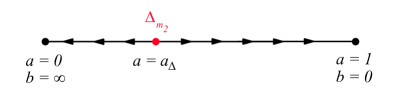
Figure 2. Flow on moduli space of one-dimensional Ising models

Recall the topological boundary theories (3.9). The low energy effective boundary field theory is $\mathrsfs{B}_{0}$ for the low temperature phase and $\mathrsfs{B}_{\mbox{$\raisebox{-0.49005pt}{\rotatebox{9.0}{\tiny/}}\mu\raisebox{-2.95358pt}{\scalebox{2.0}{$\color[rgb]{1,1,1}.$}}\raisebox{2.65222pt}{$\color[rgb]{1,1,1}.$}\hskip 3.22005pt$}_{2}}$ for the high temperature phase. We worked out the values on $S^{1}$ in Example 3.50. Recall that $\mathrsfs{B}(S^{1})$ is an object in the category $\mathrsfs{G}_{\mbox{$\raisebox{-0.49005pt}{\rotatebox{9.0}{\tiny/}}\mu\raisebox{-2.95358pt}{\scalebox{2.0}{$\color[rgb]{1,1,1}.$}}\raisebox{2.65222pt}{$\color[rgb]{1,1,1}.$}\hskip 3.22005pt$}_{2}}(S^{1})$ of $\mbox{$\raisebox{-0.70007pt}{\rotatebox{9.0}{\tiny/}}\mu\raisebox{-4.2194pt}{\scalebox{2.0}{$\color[rgb]{1,1,1}.$}}\raisebox{3.7889pt}{$\color[rgb]{1,1,1}.$}\hskip 4.60007pt$}_{2}$-equivariant vector bundles over $\mbox{$\raisebox{-0.70007pt}{\rotatebox{9.0}{\tiny/}}\mu\raisebox{-4.2194pt}{\scalebox{2.0}{$\color[rgb]{1,1,1}.$}}\raisebox{3.7889pt}{$\color[rgb]{1,1,1}.$}\hskip 4.60007pt$}_{2}$, so a pair $V_{1},V_{-1}$ of representations of $\mbox{$\raisebox{-0.70007pt}{\rotatebox{9.0}{\tiny/}}\mu\raisebox{-4.2194pt}{\scalebox{2.0}{$\color[rgb]{1,1,1}.$}}\raisebox{3.7889pt}{$\color[rgb]{1,1,1}.$}\hskip 4.60007pt$}_{2}$. The underlying vector spaces are the vacuum states of the Ising theory in the untwisted ($V_{1}$) and twisted ($V_{-1}$) sectors; the $\mbox{$\raisebox{-0.70007pt}{\rotatebox{9.0}{\tiny/}}\mu\raisebox{-4.2194pt}{\scalebox{2.0}{$\color[rgb]{1,1,1}.$}}\raisebox{3.7889pt}{$\color[rgb]{1,1,1}.$}\hskip 4.60007pt$}_{2}$-action is that of the global symmetry which reverses all of the classical spins simultaneously.

For the low temperature phase the low energy field theory is $\mathrsfs{B}=\mathrsfs{B}_{0}$. The untwisted space  $V_{1}$ is the regular representation of $\mbox{$\raisebox{-0.70007pt}{\rotatebox{9.0}{\tiny/}}\mu\raisebox{-4.2194pt}{\scalebox{2.0}{$\color[rgb]{1,1,1}.$}}\raisebox{3.7889pt}{$\color[rgb]{1,1,1}.$}\hskip 4.60007pt$}_{2}$, which is realized as the space of functions on a set of two points which are exchanged by the $\mbox{$\raisebox{-0.70007pt}{\rotatebox{9.0}{\tiny/}}\mu\raisebox{-4.2194pt}{\scalebox{2.0}{$\color[rgb]{1,1,1}.$}}\raisebox{3.7889pt}{$\color[rgb]{1,1,1}.$}\hskip 4.60007pt$}_{2}$-action. For each polygon $\Pi\subset S^{1}$ the configuration set of the Ising model is the set of functions $s\colon\operatorname{Vert}(\Pi)\to\mbox{$\raisebox{-0.70007pt}{\rotatebox{9.0}{\tiny/}}\mu\raisebox{-4.2194pt}{\scalebox{2.0}{$\color[rgb]{1,1,1}.$}}\raisebox{3.7889pt}{$\color[rgb]{1,1,1}.$}\hskip 4.60007pt$}_{2}$; the two-element vacuum set is the subset of constant functions, exchanged by the global symmetry. The two-dimensional vector space $V_{1}$ is the lowest eigenspace of the untwisted Hamiltonian. The twisted space $V_{-1}$ is the zero vector space. In the twisted sector there are many classical configurations $s$ of small energy—after trivializing the nontrivial double cover $R\to S^{1}$ on $S^{1}\setminus\{p\}$ for $p\in S^{1}\setminus\operatorname{Vert}(\Pi)$ they each have a single vertex in $\Pi$ at which $s$ takes a value distinct from that at the other vertices. The lowest energy quantum state is the equally weighted superposition; the indicator function of this subset of configurations. Its energy is strictly larger than the minimal energy in the untwisted sector. At low temperature the energy differences persist independent of $\Pi$, which leads to the vanishing of $V_{-1}$.

By contrast, in the high temperature phase the energy differences do not persist as the lattice $\Pi$ is refined; note they are completely absent at $a=1$. The low energy theory $\mathrsfs{B}=\mathrsfs{B}_{\mbox{$\raisebox{-0.49005pt}{\rotatebox{9.0}{\tiny/}}\mu\raisebox{-2.95358pt}{\scalebox{2.0}{$\color[rgb]{1,1,1}.$}}\raisebox{2.65222pt}{$\color[rgb]{1,1,1}.$}\hskip 3.22005pt$}_{2}}$ has $V_{1},V_{-1}$ each the trivial one-dimensional representation of $\mbox{$\raisebox{-0.70007pt}{\rotatebox{9.0}{\tiny/}}\mu\raisebox{-4.2194pt}{\scalebox{2.0}{$\color[rgb]{1,1,1}.$}}\raisebox{3.7889pt}{$\color[rgb]{1,1,1}.$}\hskip 4.60007pt$}_{2}$; the symmetry is unbroken in each sector. The vacuum state of the quantum theory on $(S^{1},\Pi)$ is an equal mixture of all classical configurations $s\colon\operatorname{Vert}(\Pi)\to\mbox{$\raisebox{-0.70007pt}{\rotatebox{9.0}{\tiny/}}\mu\raisebox{-4.2194pt}{\scalebox{2.0}{$\color[rgb]{1,1,1}.$}}\raisebox{3.7889pt}{$\color[rgb]{1,1,1}.$}\hskip 4.60007pt$}_{2}$, the constant function on the configuration set. This is true in both sectors—at high temperature the global twisting of the double cover does not affect the behavior of the Hamiltonian on $S^{1}$.

6. The regular topological boundary theory

In this section we illustrate computations in an extended field theory with boundary conditions and domain walls. We use some of these results in §7. We begin in §6.1 with a review of oriented 2-dimensional extended field theories. Then in §6.2 we consider a 3-dimensional theory based on a spherical fusion category, emphasizing the utility of the regular (Dirichlet) boundary theory (Remark 2.9).

6.1. 2-dimensional extended field theories

We summarize some aspects of [MS]; see also [La] and [L, §4.2].

Let $C$ be a semisimple linear category with finitely many simple objects. A Frobenius structure (or Calabi-Yau structure) on $C$ is a collection of nondegenerate traces

(6.1) $$\tau_{x}\colon\operatorname{End}^{\vphantom{1*\prime y\vee M}}_{C}(x)\longrightarrow{\mathbb{C}},\qquad x\in C,$$

which for every sequence

(6.2) $$x_{0}\xrightarrow{\;\;f_{0}\;\;}x_{1}\xrightarrow{\;\;f_{1}\;\;}x_{2}\longrightarrow\;\cdots\;\xrightarrow{\;\;f_{k-1}\;\;}x_{k}\xrightarrow{\;\;f_{k}\;\;}x_{0}$$

of morphisms in $C$ satisfy: $\tau_{x_{i}}(f_{i+k}\cdots f_{i+1}f_{i})$ is independent of $i=0,\dots,k$. (Set $f_{i+k+1}=f_{i}$ for $i=0,\dots,k-1$.) Equivalent data is a nondegenerate trace $\tau\colon HH_{0}(C)\to{\mathbb{C}}$ on the Hochschild homology. Let $x_{1},\dots,x_{N}$ be a representative set of simple objects. The data of $\tau$ amounts to $N$ complex numbers

(6.3) $$\lambda_{i}=\tau_{x_{i}}(\operatorname{id}_{x_{i}}),\qquad i=1,\dots,N.$$

The finite semisimple category $C$ is 2-dualizable in the 2-category $\mathscr{C}at=\mathscr{C}at_{{\mathbb{C}}}$ of complex linear categories, and a Frobenius structure is precisely $SO_{2}$-invariance data. By the cobordism hypothesis there is an associated 2-dimensional topological field theory

(6.4) $$\mathrsfs{T}^{\vphantom{1*\prime y\vee M}}_{\!C}\colon\operatorname{Bord}_{2}(SO_{2})\longrightarrow\mathscr{C}at$$

of oriented manifolds with $\mathrsfs{T}^{\vphantom{1*\prime y\vee M}}_{\!C}(\operatorname{pt})=C$. An object $x\in C$ is the image of ${\mathbb{C}}\in\mathscr{V}ect$ under a morphism $\mathscr{V}ect\to C$ in $\mathscr{C}at$. Apply the cobordism hypothesis to construct a boundary theory $\mathrsfs{B}_{x}\colon 1\to\mathrsfs{T}^{\vphantom{1*\prime y\vee M}}_{\!C}$. The pair $(\mathrsfs{T}^{\vphantom{1*\prime y\vee M}}_{\!C},\mathrsfs{B}_{x})$ maps the bordism (i) in Figure 3 to the object $x\in C$.

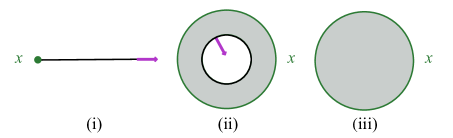
Figure 3. Three bordisms with boundary theory labeled by $x\in C$. The arrows indicate incoming vs. outgoing boundary components.

The vector space $A=\mathrsfs{T}^{\vphantom{1*\prime y\vee M}}_{\!C}(S^{1})$ is a commutative Frobenius algebra. Multiplication is $\mathrsfs{T}^{\vphantom{1*\prime y\vee M}}_{\!C}$  applied to a pair of pants, the trace $\tau_{A}\colon A\to{\mathbb{C}}$ is $\mathrsfs{T}^{\vphantom{1*\prime y\vee M}}_{\!C}$ applied to a 2-disk $D^{2}$ with $\partial D^{2}$ outgoing, and the identity element $\operatorname{id}_{A}$ is $\mathrsfs{T}^{\vphantom{1*\prime y\vee M}}_{\!C}$ applied to $D^{2}$ with $\partial D^{2}$ incoming. There is a vector space basis $e_{1},\dots,e_{N}$ of $A$ consisting of idempotents; the order is not canonical. The identity element is $\operatorname{id}_{A}=e_{1}+\cdots+e_{N}$ and

(6.5) $$\tau_{A}(e_{i})=\lambda_{i}^{2},\qquad i=1,\dots,N.$$

If $\mathcal{O}(C)$ is the finite set of isomorphism classes of simple objects in $C$, then we can identify $C=\mathscr{V}ect\bigl{(}\mathcal{O}(C)\bigr{)}$ as the category of vector bundles on $\mathcal{O}(C)$ and $A=\operatorname{Fun}\bigl{(}\mathcal{O}(C)\bigr{)}$ as the commutative algebra of functions on $\mathcal{O}(C)$. Suppose the label ‘$x$’ in the last two bordisms of Figure 3 is a $\delta$-function at $e_{i}\in A$. Then bordism (ii) evaluates to an element $\chi_{i}\in A$, which by [MS, (2,36)] is

(6.6) $$\chi_{i}=\frac{e_{i}}{\lambda_{i}}.$$

Hence bordism (iii) evaluates to

(6.7) $$\tau_{A}(\chi_{i})=\lambda_{i}.$$

The partition function of a closed oriented surface $Y$ is computed by Verlinde’s formula

(6.8) $$\mathrsfs{T}^{\vphantom{1*\prime y\vee M}}_{\!C}(Y)=\sum\limits_{i=1}^{N}\lambda_{i}^{\operatorname{Euler}(Y)}.$$

In particular,

(6.9) $$\mathrsfs{T}^{\vphantom{1*\prime y\vee M}}_{\!C}(S^{2})=\sum\limits_{i=1}^{N}\lambda_{i}^{2},$$

which follows by decomposing the bordism $S^{2}\colon\emptyset^{1}\to\emptyset^{1}$ as the composition $\emptyset^{1}\xrightarrow{\;D^{2}\;}S^{1}\xrightarrow{\;D^{2}\;}\emptyset^{1}$, from which we conclude $\mathrsfs{T}^{\vphantom{1*\prime y\vee M}}_{\!C}(S^{2})=\tau_{A}(\operatorname{id}_{A})$.

6.2. Computations in 3-dimensional extended field theories

Let $\mathscr{T}$ be a spherical fusion category and

(6.10) $$\mathrsfs{F}^{\vphantom{1*\prime y\vee M}}_{\!\mathscr{T}}\colon\operatorname{Bord}_{3}(SO_{3})\longrightarrow\mathscr{T}ens\mathscr{C}at$$

the associated 3-dimensional topological field theory of oriented manifolds with $\mathrsfs{F}^{\vphantom{1*\prime y\vee M}}_{\!\mathscr{T}}(\operatorname{pt})=\mathscr{T}$. Recall (Remark 2.9) that a left $\mathscr{T}$-module $\mathscr{L}$ is a morphism $\mathscr{L}\colon 1\to\mathscr{T}$ in $\mathscr{T}ens\mathscr{C}at$. If the underlying category of $\mathscr{L}$ is semisimple with finitely many simple objects, then $\mathscr{L}$ is 2-dualizable. To define a boundary theory $\mathrsfs{B}^{\vphantom{1*\prime y\vee M}}_{\!\mathscr{L}}\colon 1\to\mathrsfs{F}^{\vphantom{1*\prime y\vee M}}_{\!\mathscr{T}}$ of oriented manifolds we need $SO_{2}$-invariance data on $\mathscr{L}$ as an $\mathscr{T}$-module. We call this a relative Frobenius structure on $\mathscr{L}$; it is relative to the pivotal structure on $\mathscr{T}$. As in [EGNO, §7.12] let $\mathscr{E}(\mathscr{L})=\operatorname{End}_{\mathscr{T}}(\mathscr{L})$ be the tensor category of $\mathscr{T}$-module functors $\mathscr{L}\to\mathscr{L}$. Then a relative Frobenius structure is a nondegenerate trace on the vector space $\operatorname{End}_{\mathscr{E}(\mathscr{L})}(1)$, where $1\subset\mathscr{E}(\mathscr{L})$ is the unit object.

Specialize to the regular boundary theory with $\mathscr{L}=\mathscr{T}$ as a left $\mathscr{T}$-module. Then $\mathscr{E}(\mathscr{T})$ is identified with $\mathscr{T}$ (acting by right multiplication on $\mathscr{T}$), and a relative Frobenius structure is a nondegenerate trace on $\operatorname{End}^{\vphantom{1*\prime y\vee M}}_{\mathscr{T}}(1)$. Since we assume $\mathscr{T}$ is fusion, $\operatorname{End}^{\vphantom{1*\prime y\vee M}}_{\mathscr{T}}(1)$ is a 1-dimensional vector space with canonical basis $\operatorname{id}_{1}$. Thus we define the canonical relative Frobenius structure on $\mathscr{T}$ to be the trace with value 1 on $\operatorname{id}_{1}\in\operatorname{End}^{\vphantom{1*\prime y\vee M}}_{\mathscr{T}}(1)$.

Remark 6.11.

For each object $x\in\mathscr{T}$ the pivotal structure $\rho$ determines a linear map $\operatorname{End}^{\vphantom{1*\prime y\vee M}}_{\mathscr{T}}(x)\to\operatorname{End}^{\vphantom{1*\prime y\vee M}}_{\mathscr{T}}(1)$ which sends $f\in\operatorname{End}^{\vphantom{1*\prime y\vee M}}_{\mathscr{T}}(x)$ to (compare (2.4))

(6.12) $$1\xrightarrow{\;\;\operatorname{coev}_{x}\;\;}x\otimes x^{\vee}\xrightarrow{\;\;f\otimes\operatorname{id}\;\;}x\otimes x^{\vee}\xrightarrow{\;\;\rho_{x}\otimes\operatorname{id}\;\;}x^{\vee\vee}\otimes x^{\vee}\xrightarrow{\;\;\operatorname{ev}_{x^{\vee}}\;\;}1$$

Therefore, a relative Frobenius structure determines a Frobenius structure on the category underlying $\mathscr{T}$. In the sequel we use the canonical choice.

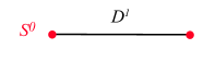
Figure 4. $D^{1}$ with boundary colored red by the regular boundary theory

It is convenient to make pictorial computations for the pair $(\mathrsfs{F}^{\vphantom{1*\prime y\vee M}}_{\!\mathscr{T}},\mathrsfs{B}^{\vphantom{1*\prime y\vee M}}_{\mathscr{T}})$. For example, consider the oriented interval $D^{1}$ with boundary $\partial D^{1}=S^{0}$ “colored” by the boundary theory $\mathrsfs{B}^{\vphantom{1*\prime y\vee M}}_{\mathscr{T}}$, as rendered in Figure 4. To interpret it we first ignore the boundary theory, read $D^{1}$ as a bordism $\operatorname{pt}\amalg\operatorname{pt}\to\emptyset^{0}$, and apply $\mathrsfs{F}^{\vphantom{1*\prime y\vee M}}_{\!\mathscr{T}}$ to obtain the functor

(6.13) $$\mathscr{T}\textnormal{-mod}\times\mathscr{T}\textnormal{-mod} \longrightarrow\mathscr{C}at$$

$$\mathscr{L}_{1}\quad,\;\quad\mathscr{L}_{2} \longmapsto\operatorname{Hom}_{\mathscr{T}}(\mathscr{L}_{1},\mathscr{L}_{2})$$

Imposing the boundary condition amounts to setting $\mathscr{L}_{1}=\mathscr{L}_{2}=\mathscr{T}$, thus we obtain the linear category underlying $\mathscr{T}$.

Remark 6.14.

In $\operatorname{Bord}_{3}(SO_{3})$ we must orient the tangent bundle of every bordism $M$, stabilized to have rank 3. At an incoming boundary component $(\partial M)_{0}$, part of the data is an orientation-preserving isomorphism

(6.15) $$\underline{{\mathbb{R}}}\oplus\underline{{\mathbb{R}}^{k}}\oplus T(\partial M)_{0}\xrightarrow{\;\;\cong\;\;}\underline{{\mathbb{R}}^{k}}\oplus TM$$

of vector bundles over $(\partial M)_{0}$ which takes $1\in\underline{{\mathbb{R}}}$ to an inward pointing vector. (Here $\dim M=3-k$.) This applies to $M=D^{1}$ with both boundary points incoming, and it shows why the two boundary points can be chosen to be isomorphic objects in $\operatorname{Bord}_{3}(SO_{3})$. Note that in a 1-dimensional field theory such an oriented bordism does not exist.

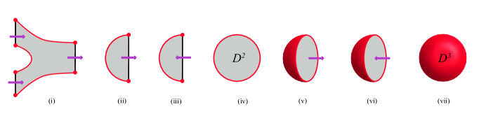
Figure 5. Seven bordisms to evaluate under $(\mathrsfs{F}^{\vphantom{1*\prime y\vee M}}_{\!\mathscr{T}},\mathrsfs{B}^{\vphantom{1*\prime y\vee M}}_{\mathscr{T}})$

Figure 5 shows seven morphisms in $\operatorname{Bord}_{3}(SO_{3})$, with parts of boundaries colored with $\mathrsfs{B}^{\vphantom{1*\prime y\vee M}}_{\mathscr{T}}$. The arrows indicate incoming vs. outgoing boundary components. We evaluate $(\mathrsfs{F}^{\vphantom{1*\prime y\vee M}}_{\!\mathscr{T}},\mathrsfs{B}^{\vphantom{1*\prime y\vee M}}_{\mathscr{T}})$ on each in turn. Bordism (i) evaluates to the tensor structure $\mathscr{T}\otimes\mathscr{T}\to\mathscr{T}$. Glue bordism (ii) to an input of bordism (i) to deduce that it evaluates to the tensor unit $1\in\mathscr{T}$. Morphism (iii) evaluates to the linear functor

(6.16) $$\mathscr{T} \longrightarrow\mathscr{V}ect$$

$$y \longmapsto\operatorname{Hom}_{\mathscr{T}}(1,y)$$

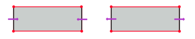
Figure 6. Evaluation and coevaluation

This follows from the evaluation and coevaluation in Figure 6—duality data for the underlying category $\mathscr{T}$—and this can be done in the dimensional reduction $\mathrsfs{T}^{\vphantom{1*\prime y\vee M}}_{\mathscr{T}}$ below. Continuing, we see bordism (iv) in Figure 5 evaluates to the vector space $\operatorname{End}^{\vphantom{1*\prime y\vee M}}_{\mathscr{T}}(1)$; bordism (v) to $\operatorname{id}_{1}\in\operatorname{End}^{\vphantom{1*\prime y\vee M}}_{\mathscr{T}}(1)$; bordism (vi) to the (canonical) relative Frobenius trace on $\operatorname{End}^{\vphantom{1*\prime y\vee M}}_{\mathscr{T}}(1)$; and bordism (vii) to the number 1, by the normalization in the canonical relative Frobenius structure.

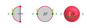
Figure 7. Three bordisms with domain wall labeled by $x\in\mathscr{T}$

Tensoring on the right by an object $x\in\mathscr{T}$ defines a left $\mathscr{T}$-module map $\mathscr{T}\to\mathscr{T}$. By the cobordism hypothesis this determines a domain wall $\mathrsfs{D}^{\vphantom{1*\prime y\vee M}}_{\phantom{W}\!\!\!\!\!\!\!x}\colon\mathrsfs{B}^{\vphantom{1*\prime y\vee M}}_{\mathscr{T}}\to\mathrsfs{B}^{\vphantom{1*\prime y\vee M}}_{\mathscr{T}}$. Consider the three bordisms in Figure 7. We co-orient the codimension two submanifold labeled $x$ inside the codimension one boundary; the co-orientation indicates the direction of the domain wall. By cutting as in Figure 5 we evaluate bordism (i) to the object $x\in\mathscr{T}$, bordism (ii) to the vector space $\operatorname{End}^{\vphantom{1*\prime y\vee M}}_{\mathscr{T}}(x)$, and bordism (iii) to the number $\dim(x)$. For the latter we see first that bordism (iii) is the canonical trace of $\operatorname{End}^{\vphantom{1*\prime y\vee M}}_{\mathscr{T}}(x)$ applied to $\operatorname{id}_{x}$. Comparing (6.12) with (2.4) we compute it to be $\dim(x)$.

Dimensional reduction of $\mathrsfs{F}^{\vphantom{1*\prime y\vee M}}_{\!\mathscr{T}}$ along the bordism $b$ in Figure 4 is a 2-dimensional oriented theory

(6.17) $$\mathrsfs{T}^{\vphantom{1*\prime y\vee M}}_{\mathscr{T}}\colon\operatorname{Bord}_{2}(SO_{2})\longrightarrow\mathscr{C}at$$

with $\mathrsfs{T}^{\vphantom{1*\prime y\vee M}}_{\mathscr{T}}(\operatorname{pt})=\mathrsfs{F}^{\vphantom{1*\prime y\vee M}}_{\!\mathscr{T}}(b)=\mathscr{T}$.

Proposition 6.18.

$\mathrsfs{T}^{\vphantom{1*\prime y\vee M}}_{\mathscr{T}}$  induces the Frobenius structure $\tau$ on the category  $\mathscr{T}$ which satisfies

(6.19) $$\tau_{x}(\operatorname{id}_{x})=\dim(x)$$

for each object $x\in\mathscr{T}$

Stated differently, $\tau$ is the canonical relative Frobenius structure on $\mathscr{T}$.

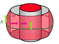
Figure 8. A decomposition of Figure 7(iii)

Proof.

The object $x\in\mathscr{T}$ determines the boundary condition $\mathrsfs{B}_{x}$ for $\mathrsfs{T}^{\vphantom{1*\prime y\vee M}}_{\mathscr{T}}$ (Figure 3(i)) which corresponds to the domain wall $\mathrsfs{D}^{\vphantom{1*\prime y\vee M}}_{\phantom{W}\!\!\!\!\!\!\!x}$ in $(\mathrsfs{F}^{\vphantom{1*\prime y\vee M}}_{\!\mathscr{T}},\mathrsfs{B}^{\vphantom{1*\prime y\vee M}}_{\mathscr{T}})$ depicted in Figure 7(i). Evaluate Figure 7(iii) by decomposing as in Figure 8. The outer spherical annulus evaluates to the image of $x$ in the commutative Frobenius algebra $\mathrsfs{T}^{\vphantom{1*\prime y\vee M}}_{\mathscr{T}}(S^{1})$. The inner solid cylinder evaluates to the trace on $\mathrsfs{T}^{\vphantom{1*\prime y\vee M}}_{\mathscr{T}}(S^{1})$. On the other hand, we already evaluated Figure 7(iii) as $\dim(x)$. Now (6.19) follows from (6.7). ∎

Recall that $\mathcal{O}(\mathscr{T})$ is the finite set of isomorphism classes of simple objects in $\mathscr{T}$.

Proposition 6.20.

(6.21) $$\mathrsfs{F}^{\vphantom{1*\prime y\vee M}}_{\!\mathscr{T}}(S^{3})=\frac{1}{\sum\limits_{x\in\mathcal{O}(\mathscr{T})}\!\!\!\!{\dim(x)^{2}}^{\phantom{W}}}.$$

A corollary is that the denominator—the categorical dimension

(6.22) $$d(\mathscr{T})=\sum\limits_{x\in\mathcal{O}(\mathscr{T})}\!\!\dim(x)^{2}$$

of $\mathscr{T}$—is nonzero, a known result [EGNO, Theorem 7.21.12].

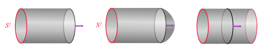
Figure 9. Three more bordisms with boundary theory

Proof.

First, $\mathrsfs{F}^{\vphantom{1*\prime y\vee M}}_{\!\mathscr{T}}(S^{2})$ is a commutative Frobenius algebra. Let $\sigma\colon\mathrsfs{F}^{\vphantom{1*\prime y\vee M}}_{\!\mathscr{T}}(S^{2})\to{\mathbb{C}}$ denote its trace. There is an algebra isomorphism $\mathrsfs{F}^{\vphantom{1*\prime y\vee M}}_{\!\mathscr{T}}(S^{2})\cong\operatorname{End}^{\vphantom{1*\prime y\vee M}}_{\mathscr{Z}(\mathscr{T})}(1)$, where $\mathscr{Z}(\mathscr{T})=\mathrsfs{F}^{\vphantom{1*\prime y\vee M}}_{\!\mathscr{T}}(S^{1})$ is the Drinfeld center of $\mathscr{T}$. The latter is 1-dimensional, since $\operatorname{End}^{\vphantom{1*\prime y\vee M}}_{\mathscr{T}}(1)$ is, and has canonical basis the unit $u\in\mathrsfs{F}^{\vphantom{1*\prime y\vee M}}_{\!\mathscr{T}}(S^{2})$. Then $\mathrsfs{F}^{\vphantom{1*\prime y\vee M}}_{\!\mathscr{T}}(S^{3})=\sigma(u)$. Bordism (i) in Figure 9 evaluates to a vector $du$ for some $d\in{\mathbb{C}}$. Use bordism (ii) to prove $\sigma(u)=d^{-1}$, since bordism (vii) in Figure 5 evaluates to the number 1. Bordism (iii) in Figure 9 evaluates to $d^{2}\sigma(u)=d$, but as it is the product of the bordism $b$ of Figure 4 with $S^{2}$ it also evaluates to

(6.23) $$\mathrsfs{T}^{\vphantom{1*\prime y\vee M}}_{\mathscr{T}}(S^{2})=\sum\limits_{x\in\mathcal{O}(\mathscr{T})}\dim(x)^{2}=d(\mathscr{T}),$$

according to (6.9). ∎

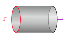
Figure 10. A special element of $\mathscr{Z}(\mathscr{T})$

Finally, we observe that $(\mathrsfs{F}^{\vphantom{1*\prime y\vee M}}_{\!\mathscr{T}},\mathrsfs{B}^{\vphantom{1*\prime y\vee M}}_{\mathscr{T}})$ maps the bordism in Figure 10 to a distinguished object in $\mathrsfs{F}^{\vphantom{1*\prime y\vee M}}_{\!\mathscr{T}}(S^{1})=\mathscr{Z}(\mathscr{T})$. Its simple constituents generate a subcategory of “abstract Wilson loop operators”.

7. Nonabelian lattice models and duality

Fix a spherical fusion category $\mathscr{T}$. The cobordism hypothesis associates to $\mathscr{T}$ an extended 3-dimensional topological field theory $\mathrsfs{F}^{\vphantom{1*\prime y\vee M}}_{\!\mathscr{T}}$ of oriented manifolds. This is the Turaev-Viro theory [TV, BW1, BW2] as generalized by Barrett-Westbury. It has a state sum formulation. In principle the state sum can be derived from the extended field theory structure, so ultimately from the cobordism hypothesis; see [Da] for a careful treatment of state sums in 2-dimensional extended oriented field theories. In §7.1 we state the relevant formulas for Turaev-Viro theory, mostly following [BK]. Then in §7.2 we construct a boundary theory for latticed manifolds, at least on closed oriented latticed 2-manifolds. For $\mathscr{T}=\mathscr{V}ect[G]$ we recover the finite gauge theory of §4. Applied to $\mathscr{T}=\mathscr{R}ep(G)$ we obtain a (Kramers-Wannier) dual to the $G$-Ising model for all finite groups $G$, including $G$ nonabelian.

7.1. Turaev-Viro theory

Let $\mathscr{T}$ be a spherical fusion category. For objects $x_{1},\dots,x_{n}\in\mathscr{T}$ define the vector space

(7.1) $$\langle x_{1},\dots,x_{n}\rangle=\operatorname{Hom}^{\vphantom{1*\prime y\vee M}}_{\mathscr{T}}(1,x_{1}\otimes\cdots\otimes x_{n}),$$

where $1\in\mathscr{T}$ is the tensor unit. Then the pivotal structure produces an isomorphism

(7.2) $$\langle x_{1},\dots,x_{n}\rangle\xrightarrow{\;\;\cong\;\;}\operatorname{Hom}^{\vphantom{1*\prime y\vee M}}_{\mathscr{T}}(x_{1}^{\vee},x_{2}\otimes\cdots\otimes x_{n})\xrightarrow{\;\;\cong\;\;}\langle x_{2},\dots,x_{n},x_{1}\rangle$$

whose $n^{\textnormal{th}}$ power is the identity. Therefore, $\langle x_{1},\dots,x_{n}\rangle$ depends only on the set of cyclically ordered objects $x_{1},\dots,x_{n}$. Furthermore, for $x_{i},y_{i},z\in\mathscr{T}$ there is a pairing

(7.3) $$\langle x_{1},\dots,x_{n},z^{\vee}\rangle\otimes\langle z,y_{1},\dots,y_{m}\rangle\longrightarrow\langle x_{1},\dots,x_{n},y_{1},\dots,y_{m}\rangle$$

defined by tensoring $\operatorname{Hom}^{\vphantom{1*\prime y\vee M}}_{\mathscr{T}}$ spaces and contracting via evaluation $z^{\vee}\otimes z\to 1$. For any $x_{1},\dots,x_{n}\in\mathscr{T}$ the pairing

(7.4) $$\langle x_{n}^{\vee},\dots,x_{1}^{\vee}\rangle\otimes\langle x_{1},\dots,x_{n}\rangle\longrightarrow\operatorname{End}^{\vphantom{1*\prime y\vee M}}_{\mathscr{T}}(1)\longrightarrow{\mathbb{C}}$$

is nondegenerate. The second arrow is the canonical relative Frobenius structure defined in §6.2. Henceforth, we restrict to simple objects of $\mathscr{T}$.

Suppose $(Y,\Lambda)$ is a closed oriented latticed 2-manifold. Let $\operatorname{OEdge}(\Lambda)$ be the set of pairs $e=(\bar{e},\mathfrak{o})$ in which $\bar{e}\in\operatorname{Edge}(\Lambda)$ and $\mathfrak{o}$ is an orientation of $\bar{e}$. Let $-e$ denote the oppositely oriented edge to $e$. Define a labeling as a function

(7.5) $$\ell\colon\operatorname{OEdge}(\Lambda)\longrightarrow\operatorname{Obj}\mathscr{T}$$

which satisfies: $\ell(e)$ is a simple object for all $e\in\operatorname{OEdge}(\Lambda)$, and $\ell(-e)=\ell(e)^{\vee}$. We say labelings $\ell\sim\ell^{\prime}$ are equivalent if $\ell(e)\cong\ell^{\prime}(e)$ for all $e\in\operatorname{OEdge}(\Lambda)$. Define the vector space [BK, (3.2.2)]

(7.6) $$V^{\vphantom{1*\prime y\vee M}}_{\mathscr{T}}(Y;\Lambda)\cong\bigoplus\limits_{\ell}\bigotimes\limits_{f}\;\langle\ell(e_{1}),\dots,\ell(e_{n})\rangle,$$

where the direct sum is over equivalence classes of labelings $\ell$, the tensor product over faces $f$ of $\Lambda$, and the boundary of a face $f$ is an $n$-gon with edges $e_{1},\dots,e_{n}$ cyclically ordered and oriented as the boundary of $f$. It has the following interpretation in the extended field theory $\mathrsfs{F}^{\vphantom{1*\prime y\vee M}}_{\!\mathscr{T}}$. Namely, as in §6 let $\mathrsfs{B}^{\vphantom{1*\prime y\vee M}}_{\mathscr{T}}$ be the regular boundary theory defined by $\mathscr{T}$ as a left module over itself. Excise open disks about each vertex of $\Lambda$ to obtain a surface $Y^{\prime}$; insert the regular boundary theory $\mathrsfs{B}^{\vphantom{1*\prime y\vee M}}_{\mathscr{T}}$ on $\partial Y^{\prime}$. Then $\mathrsfs{F}^{\vphantom{1*\prime y\vee M}}_{\!\mathscr{T}}(Y^{\prime})$ is the vector space (7.6), as we briefly explain. Compute $\mathrsfs{F}^{\vphantom{1*\prime y\vee M}}_{\!\mathscr{T}}(Y^{\prime})$ by cutting along each edge of $\Lambda\cap Y^{\prime}$ to decompose $Y^{\prime}$ as a union of polygons with vertices blown-up to arcs colored with $\mathrsfs{B}^{\vphantom{1*\prime y\vee M}}_{\mathscr{T}}$; see Figure 11. Each such polygon evaluates to a vector space (7.1), once labels are inserted on the edges. Evaluation of the thin rectangles attached to doubled edges leads to the sum and product in (7.6).

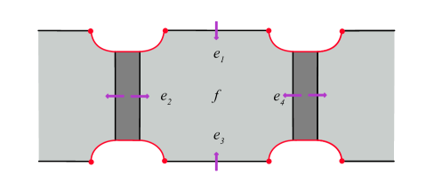
Figure 11. The blown-up lattice

Example 7.7 ($\mathscr{T}={\mathscr{V}ect[G]}$).

A simple object is a “skyscraper vector bundle”, a line supported at a single element $g\in G$. Hence an equivalence class of labelings is a function $g\colon\operatorname{OEdge}(\Lambda)\to G$ such that $g(-e)=g(e)^{-1}$. Let ${\mathbb{C}}_{g}$ be the skyscraper trivial line supported at $g$ and $*$ the convolution product (3.3). We easily compute the vector space

(7.8) $$\langle g_{1},\dots,g_{n}\rangle=\operatorname{Hom}^{\vphantom{1*\prime y\vee M}}_{\mathscr{V}ect[G]}(1,{\mathbb{C}}_{g_{1}}*\cdots*{\mathbb{C}}_{g_{n}})=\begin{cases}{\mathbb{C}},&g_{1}\cdots g_{n}=e;\\ 0,&\textnormal{otherwise}.\end{cases}$$

The set of labelings is equivalent to the groupoid of principal $G$-bundles over $\Lambda$ together with a section over $\operatorname{Vert}(\Lambda)$; the equivalence is parallel transport along edges. (Recall that the section over vertices is the canonical Dirichlet boundary theory; see the end of §3.1.) According to (7.8) the vector space in (7.6) for fixed $\ell,f$ is zero unless the holonomy around the face $f$ is trivial. Therefore, we can identify (7.6) with the vector space of functions on $\operatorname{Bun}_{G}(Y,\operatorname{Vert}(\Lambda))$, the stack of $G$-bundles on $Y$ trivialized at vertices of $\Lambda$.

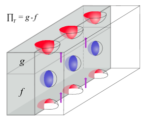
Figure 12. A schematic of the bordism $\Pi^{\vphantom{1*\prime y\vee M}}_{Y}=g\circ f$ with blue antispheres

To compute the vector space $\mathrsfs{F}^{\vphantom{1*\prime y\vee M}}_{\!\mathscr{T}}(Y)$ we must glue back in the excised disks about vertices. We cannot literally do that, due to the boundary theory, so we take a different route. First, recall from the proof of Proposition 6.20 that $\mathrsfs{F}^{\vphantom{1*\prime y\vee M}}_{\!\mathscr{T}}(S^{2})$ is 1-dimensional with canonical basis element $u$. Furthermore, $S^{2}$ colored with the boundary theory $\mathrsfs{B}^{\vphantom{1*\prime y\vee M}}_{\mathscr{T}}$ defines the vector $d(\mathscr{T})u\in\mathrsfs{F}^{\vphantom{1*\prime y\vee M}}_{\!\mathscr{T}}(S^{2})$—this is the evaluation of the relative theory, which amounts to evaluating $(\mathrsfs{F}^{\vphantom{1*\prime y\vee M}}_{\!\mathscr{T}},\mathrsfs{B}^{\vphantom{1*\prime y\vee M}}_{\mathscr{T}})$ on bordism (i) in Figure 9—for the nonzero constant $d(\mathscr{T})$ defined in (6.22). Define the “antisphere” to be a colored $S^{2}$ postulated to have value $d(\mathscr{T})^{-1}u\in\mathrsfs{F}^{\vphantom{1*\prime y\vee M}}_{\!\mathscr{T}}(S^{2})$. Now define a bordism $\Pi^{\vphantom{1*\prime y\vee M}}_{Y}\colon Y^{\prime}\to Y^{\prime}$ as the manifold $[0,1]\times Y$ with, for each $v\in\operatorname{Vert}(\Lambda)$; a “hemiball” removed about each vertex $\{0\}\times v$, $\{1\}\times v$ at the boundary; and a small ball removed at $\{1/4\}\times v$ with boundary an antisphere. Put the boundary theory $\mathrsfs{B}^{\vphantom{1*\prime y\vee M}}_{\mathscr{T}}$ on the hemisphere boundary of each excised hemiball. Figure 12 is a 2-dimensional slice through $\Pi^{\vphantom{1*\prime y\vee M}}_{Y}$. The theory $\mathrsfs{F}^{\vphantom{1*\prime y\vee M}}_{\!\mathscr{T}}$ evaluates on each end of $\Pi^{\vphantom{1*\prime y\vee M}}_{Y}$ to the vector space $\mathrsfs{F}^{\vphantom{1*\prime y\vee M}}_{\!\mathscr{T}}(Y^{\prime})=V^{\vphantom{1*\prime y\vee M}}_{\mathscr{T}}(Y;\Lambda)$.

Lemma 7.9.

$\mathrsfs{F}^{\vphantom{1*\prime y\vee M}}_{\!\mathscr{T}}(\Pi^{\vphantom{1*\prime y\vee M}}_{Y})\colon V^{\vphantom{1*\prime y\vee M}}_{\mathscr{T}}(Y;\Lambda)\longrightarrow V^{\vphantom{1*\prime y\vee M}}_{\mathscr{T}}(Y;\Lambda)$ is a projection with image isomorphic to $\mathrsfs{F}^{\vphantom{1*\prime y\vee M}}_{\!\mathscr{T}}(Y)$.

Proof.

The composition $\Pi^{\vphantom{1*\prime y\vee M}}_{Y}\circ\Pi^{\vphantom{1*\prime y\vee M}}_{Y}$ in the bordism category is diffeomorphic to $\Pi^{\vphantom{1*\prime y\vee M}}_{Y}$ with (i) an interior ball excised for each $v\in\operatorname{Vert}(\Lambda)$ with boundary colored by  $\mathrsfs{B}^{\vphantom{1*\prime y\vee M}}_{\mathscr{T}}$, and (ii) two antispheres for each vertex. Use the multiplication in $\mathrsfs{F}^{\vphantom{1*\prime y\vee M}}_{\!\mathscr{T}}(S^{2})$ to cancel the $\mathrsfs{B}^{\vphantom{1*\prime y\vee M}}_{\mathscr{T}}$-sphere against one of the antispheres. To complete the proof, refer to Figure 12 and observe that $f\circ g\approx\operatorname{id}_{Y}$, after canceling the $\mathrsfs{B}^{\vphantom{1*\prime y\vee M}}_{\mathscr{T}}$-spheres against the antispheres, which implies that $\mathrsfs{F}^{\vphantom{1*\prime y\vee M}}_{\!\mathscr{T}}(g)$ is an isomorphism of $\mathrsfs{F}^{\vphantom{1*\prime y\vee M}}_{\!\mathscr{T}}(Y)$ onto the image of $\mathrsfs{F}^{\vphantom{1*\prime y\vee M}}_{\!\mathscr{T}}(\Pi^{\vphantom{1*\prime y\vee M}}_{Y})$. ∎

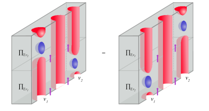
Figure 13. Commutativity of local projections

Decompose $\mathrsfs{F}^{\vphantom{1*\prime y\vee M}}_{\!\mathscr{T}}(\Pi^{\vphantom{1*\prime y\vee M}}_{Y})$ as a composition of commuting projections $\mathrsfs{F}^{\vphantom{1*\prime y\vee M}}_{\!\mathscr{T}}(\Pi^{\vphantom{1*\prime y\vee M}}_{Y,v})\colon V^{\vphantom{1*\prime y\vee M}}_{\mathscr{T}}(Y;\Lambda)\to V^{\vphantom{1*\prime y\vee M}}_{\mathscr{T}}(Y;\Lambda)$, $v\in\operatorname{Vert}(\Lambda)$, by setting

(7.10) $$\Pi^{\vphantom{1*\prime y\vee M}}_{Y,v}=[0,1]\times Y^{\prime}\cup^{\vphantom{1*\prime y\vee M}}_{[\frac{1}{16},\frac{15}{16}]\times\partial_{v}Y^{\prime}}\,\left[\frac{1}{16},\frac{15}{16}\right]\times D^{2}\;\;\setminus\;\;\left[\frac{1}{8},\frac{3}{8}\right]\times D^{2},$$

where $\partial_{v}y^{\prime}\approx S^{1}$ is the boundary of the excised ball about $v$ and the boundary of $[\frac{1}{8},\frac{3}{8}]\times D^{2}$ is the antisphere. There is a standard “picture proof” (Figure 13) that for vertices $v_{1},v_{2}$ we have

(7.11) $$\Pi^{\vphantom{1*\prime y\vee M}}_{Y,v_{1}}\circ\Pi^{\vphantom{1*\prime y\vee M}}_{Y,v_{2}}=\Pi^{\vphantom{1*\prime y\vee M}}_{Y,v_{2}}\circ\Pi^{\vphantom{1*\prime y\vee M}}_{Y,v_{1}}$$

in the bordism category.

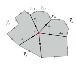
Figure 14. The labeled closed star of $v$

We conclude with a formula for $\mathrsfs{F}^{\vphantom{1*\prime y\vee M}}_{\!\mathscr{T}}(\Pi^{\vphantom{1*\prime y\vee M}}_{Y,v})$ in terms of the state sum (7.6). Figure 14 depicts the “closed star” of the vertex $v$ and defines a labeling of its edges. For any labeling $\ell$ in (7.6) with these labels, the desired projection is the identity on the vector space (7.1) associated to faces which do not contain $v$, tensored with the linear map

(7.12) $$\bigotimes\limits_{i=1}^{n}\;\langle x_{i},\vec{y}_{i},x_{i+1}^{\vee}\rangle \xrightarrow{\;\;\phantom{1/d(\mathscr{T})}\;\;}\;\bigoplus\limits_{\tilde{x}_{i},z}\,\bigotimes\limits_{i=1}^{n}\;\langle x_{i},\vec{y}_{i},x_{i+1}^{\vee}\rangle\otimes\langle x_{i},\tilde{x}_{i}^{\vee},z\rangle\otimes\langle z^{\vee},\tilde{x}_{i},x_{i}^{\vee}\rangle$$

$$\quad\;\;=\quad\;\;\bigoplus\limits_{\tilde{x}_{i},z}\,\bigotimes\limits_{i=1}^{n}\;\langle x_{i},\vec{y}_{i},x_{i+1}^{\vee}\rangle\otimes\langle x_{i+1},\tilde{x}_{i+1}^{\vee},z\rangle\otimes\langle z^{\vee},\tilde{x}_{i},x_{i}^{\vee}\rangle$$

$$\xrightarrow{\;\;\phantom{1/d(\mathscr{T})}\;\;}\;\bigoplus\limits_{\tilde{x}_{i}}\bigotimes\limits_{i=1}^{n}\;\langle\tilde{x}_{i},\vec{y}_{i},\tilde{x}_{i+1}^{\vee}\rangle$$

$$\xrightarrow{\;\;1/d(\mathscr{T})\;\;}\;\bigoplus\limits_{\tilde{x}_{i}}\bigotimes\limits_{i=1}^{n}\;\langle\tilde{x}_{i},\vec{y}_{i},\tilde{x}_{i+1}^{\vee}\rangle,$$

where we set $x_{n+1}=x_{1}$ and $\tilde{x}_{n+1}=\tilde{x}_{1}$. The first map is constructed from the dual of the duality pairing (7.4). The second map is defined using the cyclic invariance (7.2) and the pairing (7.3):

(7.13) $$\langle x_{i},\vec{y}_{i},x_{i+1}^{\vee}\rangle\otimes\langle x_{i+1}, \tilde{x}_{i+1}^{\vee},z\rangle\otimes\langle z^{\vee},\tilde{x}_{i},x_{i}^{\vee}\rangle$$

$$\longrightarrow\langle\tilde{x}_{i+1}^{\vee},z,x_{i+1}\rangle\otimes\langle x_{i+1}^{\vee},z^{\vee},\tilde{x}_{i},\vec{y}_{i}\rangle$$

$$\longrightarrow\langle\tilde{x}_{i},\vec{y}_{i},x_{i+1}^{\vee},x_{i+1},\tilde{x}_{i+1}^{\vee}\rangle$$

$$\longrightarrow\langle\tilde{x}_{i},\vec{y}_{i},\tilde{x}_{i+1}^{\vee}\rangle$$

The last map is the indicated multiplication operator.

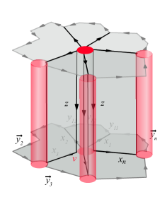
Figure 15. A small portion of $\Pi^{\vphantom{1*\prime y\vee M}}_{Y,v}$

Proposition 7.14.

The operator on $V^{\vphantom{1*\prime y\vee M}}_{\mathscr{T}}(Y;\Lambda)$ defined in (7.12) is $\mathrsfs{F}^{\vphantom{1*\prime y\vee M}}_{\!\mathscr{T}}(\Pi^{\vphantom{1*\prime y\vee M}}_{Y,v})$.

Proof.

We sketch a proof based on Figure 15 and our computations in §6.2. The left drawing depicts a decomposition of a portion of $\Pi^{\vphantom{1*\prime y\vee M}}_{Y,v}$. A solid cylinder has been bored from the north pole of the bottom hemisphere at $v$ to the south pole of the top hemisphere. Its boundary is co-oriented to point into the faces containing $v$. Edges of $\Lambda$ are doubled, as in Figure 11. Each face of appears in the decomposition of $\Pi^{\vphantom{1*\prime y\vee M}}_{Y,v}$ bounded by vertical polygons as in the right drawing; the pair $(\mathrsfs{F}^{\vphantom{1*\prime y\vee M}}_{\!\mathscr{T}},\mathrsfs{B}^{\vphantom{1*\prime y\vee M}}_{\mathscr{T}})$ maps that particular polygon to the vector space $\langle x^{\vphantom{1*\prime y\vee M}}_{i},\tilde{x}^{\vee}_{i},z\rangle$. There is a thin vertical “slab” for each edge. The vertical faces of the slabs are outgoing. The bottom face of $\Pi^{\vphantom{1*\prime y\vee M}}_{Y,v}$ is incoming and the top face outgoing, as in Figure 12. The value of $(\mathrsfs{F}^{\vphantom{1*\prime y\vee M}}_{\!\mathscr{T}},\mathrsfs{B}^{\vphantom{1*\prime y\vee M}}_{\mathscr{T}})$ on the thin vertical slabs are the coevaluation maps in the first line of (7.12). The contractions in (7.13) occur when evaluating the face along the two shown vertical polygons, bottom face, and vertical cylinder, each of which is incoming. The first contraction is gluing along $x_{i}$, the second along $z$, and the third along $x_{i+1}$. The top face being outgoing there are no contractions with the tilde variables. The vertical solid cylinder can be evaluated as a solid polygon in the reduced theory $\mathrsfs{T}^{\vphantom{1*\prime y\vee M}}_{\mathscr{T}}$ of (6.17). This enforces that all vertical variables $z$ be equal. Finally, the antisphere induces the multiplication operator at the last step of (7.12). ∎

Example 7.15 ($\mathscr{T}={\mathscr{V}ect[G]}$).

Resuming Example 7.7, we claim (7.12) projects onto functions on $\operatorname{Bun}_{G}(Y,\operatorname{Vert}(\Lambda))$ which are invariant under change of trivialization at $v$. To see this, recall that each label is a group element, note that $z\in G$ functions as the change of trivialization at $v$, and $\tilde{x}_{i}$ is determined by $x_{i}$ and $z$. Applying to all $v$ we obtain projection onto the image of

(7.16) $$\operatorname{Fun}\bigl{(}\operatorname{Bun}_{G}(Y)\bigr{)}\longrightarrow\operatorname{Fun}\bigl{(}\operatorname{Bun}_{G}(Y,\operatorname{Vert}(\Lambda))\bigr{)}.$$

7.2. The lattice boundary theory

The boundary theory depends on a fiber functor, i.e., a tensor functor

(7.17) $$\phi\colon\mathscr{T}\longrightarrow\mathscr{V}ect_{\mathbb{C}}.$$

Furthermore, we need the generalization of the Ising weight function in §4.1. First, duality is an involution on $\mathcal{O}(\mathscr{T})$. Choose representative simple objects $x_{1},\dots,x_{N}$ in $\mathscr{T}$ and duality data for dual pairs of objects. The desired weight function is an element

(7.18) $$\theta\in\bigoplus\limits_{i=1}^{N}\phi(x_{i})\otimes\phi(x_{i})^{*}$$

which satisfies the following “evenness” constraint: the duality data induces an involution of the vector space (which permutes terms), and we require that $\theta$ be invariant. We assume $\phi$ and $\theta$ are specified.

Example 7.19.

For $\mathscr{T}=\mathscr{V}ect[G]$ the fiber functor $\phi$ maps a vector bundle $W\to G$ to the vector space $\bigoplus_{g\in G}W_{g}$. If $x\in\mathscr{V}ect[G]$ is a skyscraper line supported at $g\in G$, then $\phi(x)\otimes\phi(x)^{*}$ is the trivial line ${\mathbb{C}}$, and we can identify the vector space in (7.18) with $\operatorname{Fun}(G)$. The constraint forces $\theta$  to be an even function, as in Definition 4.9.

Example 7.20.

For $\mathscr{T}=\mathscr{R}ep(G)$ the vector space in (7.18) is the home of the “Fourier transform” of a function on $G$; see (4.8).

Observe that for any object $x\in\mathscr{T}$ there is a canonical isomorphism

(7.21) $$\operatorname{Hom}\bigl{(}1,\operatorname{Hom}(1,x)^{*}\otimes x\bigr{)}\xrightarrow{\;\;\cong\;\;}\operatorname{Hom}(1,x)^{*}\otimes\operatorname{Hom}(1,x)$$

and a canonical element in the latter. Hence for a latticed surface $(Y,\Lambda)$ there is a canonical map

(7.22) $$1\longrightarrow \bigoplus\limits_{\ell}\bigotimes\limits_{f}\;\langle\ell(e_{n})^{\vee},\dots,\ell(e_{1})^{\vee}\rangle^{*}\otimes\ell(e_{n})^{\vee}\otimes\cdots\otimes\ell(e_{1})^{\vee}$$

$$\!\!\!\!\!\!\!\cong\bigoplus\limits_{\ell}\bigotimes\limits_{f}\;\;\;\;\,\langle\ell(e_{1}),\dots,\ell(e_{n})\rangle\;\;\;\otimes\ell(e_{n})^{\vee}\otimes\cdots\otimes\ell(e_{1})^{\vee},$$

where $e_{1},\dots,e_{n}$ are the edges of the $n$-gon $f$ and we use the duality pairing (7.4). Apply the fiber functor to obtain a linear map of vector spaces

(7.23) $${\mathbb{C}}\longrightarrow\bigoplus\limits_{\ell}\bigotimes\limits_{f}\;\langle\ell(e_{1}),\dots,\ell(e_{n})\rangle\otimes\phi\bigl{(}\ell(e_{n})\bigr{)}^{*}\otimes\cdots\otimes\phi\bigl{(}\ell(e_{1})\bigr{)}^{*}.$$

For a fixed labeling $\ell$, each unoriented edge $\bar{e}\in\operatorname{Edge}(\Lambda)$ appears in (7.23) twice, once with each orientation. Pair the image of $1\in{\mathbb{C}}$ under (7.23) with $\prod_{e\in\operatorname{Edge}(\Lambda)}\theta$ to obtain a vector in the vector space $V^{\vphantom{1*\prime y\vee M}}_{\mathscr{T}}(Y;\Lambda)$ of (7.6). (The constraint on $\theta$ is needed for this pairing to be well-defined.) Finally, apply the projection $\mathrsfs{F}^{\vphantom{1*\prime y\vee M}}_{\!\mathscr{T}}(\Pi^{\vphantom{1*\prime y\vee M}}_{Y})$ of Lemma 7.9 to obtain the partition function of the boundary lattice theory, a vector in $\mathrsfs{F}^{\vphantom{1*\prime y\vee M}}_{\!\mathscr{T}}(Y)$.

Example 7.24.

For $\mathscr{T}=\mathscr{V}ect[G]$ this prescription reproduces (4.21), as we encourage the reader to verify.

8. Bicolored boundary structures

Here, we give an abstract reformulation of our TQFT interpretation of the Ising model and its correlators in the setting of fully extended topological field theories recalled in §2: we will describe the data of a $d$-dimensional lattice theory relative to a $(d+1)$-dimensional topological field theory  $\mathrsfs{F}$ in the language of boundary and defect structures. Unless otherwise specified, we will dwell in the world of oriented theories.

As mentioned in the introduction, the formulation of Kramers-Wannier duality in the context of a (nonextended) bicolored TQFT is anticipated in [S].

8.1. Bi-coloring via Morse functions.

We assume at the outset that the $d$-manifold $Y$ ($d\geq 2$) carrying the lattice theory is closed. Permitted cuts of $Y$ into cornered pieces will be apparent after our reformulation: all faces of a cornered bordism must be transverse to all boundary and defect structures. Contact with the world of extended TQFTs is made by converting a lattice on $Y$ into a handle decomposition. There is a standard way to do so, once we make the notion of “lattice” precise enough. We will take it to mean a piecewise linear decomposition $\Pi$ into convex polyhedra (not necessarily simplices), compatible with the smooth structure. From this, one can build a Morse function $f$ on $Y$ in a standard way, with one critical point on each polyhedral face (including the $d$-dimensional ones). We will arrange for the Morse function to be self-indexing, with vertices of degree $0$ and maxima of degree $d$. The Morse function $d-f$ is then compatible, in the same way, with the dual polyhedral decomposition  $\Pi^{\vee}$, which itself is uniquely defined up to smooth isotopy. These constructions are readily carried out thanks to Whitehead’s results [Wh] on triangulations of $C^{1}$ manifolds.

The lattice theory on $Y$ being a boundary theory for $\mathrsfs{F}$, the associated TQFT picture is always based on a collar of $Y$ in some $(d+1)$-manifold; the topological nature of $\mathrsfs{F}$ confines all the information to a cylinder $[0,1]\times Y$, with boundary $Y_{0}\amalg Y_{1}$, with $Y_{0}$ soon to be decorated by boundary and defect structures. Its algebraic reading will output a vector in the image $\mathrsfs{F}(Y_{1})$ of the smooth boundary, but the incoming boundary $Y_{0}$ needs a preliminary change.

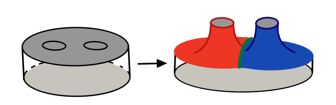
Figure 16. Modifying $[0,1]\times Y$ into a cornered bordism

The Morse function $f$ gives a handle decomposition of $Y$, with a $p$-handle $D^{p}\times D^{q}$ centered at each critical point $y$ of index $p$. Inside each handle, mark out a smaller disk $D_{y}$, whose boundary is Hopf-split into two solid tori $D^{p}\times S^{q-1}\cup S^{p-1}\times D^{q}$ glued along their boundary torus $T_{y}=S^{p-1}\times S^{q-1}$, the level-set $f=p$ in $\partial D_{y}$. We now deform the smooth structure on $[0,1]\times Y$ into a manifold $X$ with corners of co-dimension $2$, converting each copy of $D_{y}\subset Y_{0}$ into a face with corner $\partial D_{y}$; a complementary face is $Y_{0}\setminus\coprod_{y}D_{y}=:Y_{c}$ (“$Y$ chromatic”), while the output $Y_{1}$ remains smooth and closed. The pair $(X,Y_{c})$ is now a cornered bordism from $\coprod_{y}(D_{y},\partial D_{y})$ to $(Y_{1},\emptyset)$, as in Figure 16.

We will use on $Y_{c}$ two colors (red and blue) to indicate boundary theories $\mathrsfs{B},\mathrsfs{B}^{\prime}$ for $\mathrsfs{F}$, as well as a collard green colored defect $\mathrsfs{D}:\mathrsfs{B}\to\mathrsfs{B}^{\prime}$. Red and blue fill, alternately, the slices between critical level sets $f=0,\dots,d$, while green colors the level sets $f=1,\dots,d-1$. Figure 17 below gives an aerial view of the square lattice (in grey) converted by means of the Morse function $\sin x\sin y$.

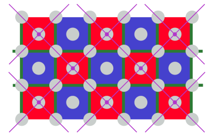
Figure 17. Converting the square lattice to a bi-colored surface

Remark 8.1 (Framings).

Recall that boundary theories, in our convention, are directed from $1$ to $\mathrsfs{F}$ (2.6). In the general setting of framed TQFTs, this convention picks the inward normal as a first vector of a $(d+1)$-framing on the red/blue parts, and a second vector tangent to the Morse flowlines on the green defect, pointing from red to green. We will specialize to oriented field theories, where we remember only orientations, with an orientation on the bulk now determines all the colored strata. Note, however, that when $d=2$, as for the Ising model, the Morse flow converts an orientation to a framing over $Y_{c}$, so in that dimension all the framing information of the theory is captured in these three handles.

The two solid tori in the boundary of each $p$-handle $D_{y}$ have opposite colors, assigned according to the parity of $p$, and separated by a green $T_{y}$. Thus colored, denote the boundary $\partial_{c}D_{y}$. Choose now a standard Euclidean model $D^{p,q}$ for this structured $D_{y}$; the quadruple $\mathrsfs{Q}:=(\mathrsfs{F},\mathrsfs{B},\mathrsfs{B}^{\prime},\mathrsfs{D})$ associates to $(D^{p,q},\partial_{c}D^{p,q})$ a vector space $H_{p}$. This space, which plays a special role as a home of the Ising action below, has a rich structure (already mentioned earlier, in §1.25); let us just mention its $E_{p}\times E_{q}$-bi-algebra structure, seen by writing $D^{p,q}=D^{p}\times D^{q}$ and multiplying in the $D^{p}$ and $D^{q}$ directions, respectively, and illustrated for $D^{1,1}$ in Figures 18 and 19 below.

After coloring $Y_{c}$, $\mathrsfs{Q}$ converts the bordism $X$ into a morphism

(8.2) $$\mathrsfs{Q}(X,Y_{c}):\bigotimes\nolimits_{y}\mathrsfs{Q}(D_{y},\partial_{c}D_{y})\to\mathrsfs{F}(Y).$$

Definition 8.3.

An Ising action for $\mathrsfs{Q}$ is a collection of vectors $\theta_{p}\in H_{p}$, each of which must be invariant under the oriented symmetry group $\mathrm{S}\left(\mathrm{O}(p)\times\mathrm{O}(q)\right)$ of $D^{p,q}$. The Ising partition function in $\mathrsfs{F}(Y)$ is the $\mathrsfs{Q}(X,Y_{c})$-image of their tensor product ranging over all handles.

Remark 8.4.

Since $H_{p}$ is a vector space and the action is topological, only the components $\{\pm 1\}$ of the symmetry group can act on it (and then only if $0<p<d$). In a derived setting, there could be additional invariance data from the continuous part of the group.

Developing this, we introduce line defects of types $0\leq p\leq d$ for $\mathrsfs{F}$, allowed to end at point defects on $Y$. Locating the latter at critical points of index $p$ allows us to promote them to “order operators of type $p$” in the lattice theory as follows. A general line defect for $\mathrsfs{F}$ is labeled by an object in the category $\mathrsfs{F}(S^{d-1})$. Such a defect requires a normal framing; to collapse the framing information to $\mathrm{SO}(d)$, or to another subgroup $S\subset\mathrm{O}(d)$, the label must be $S$-invariant.

Remark 8.5.

In the strict case, $S$ acts via its $(\pi_{0},\pi_{1})$-truncation, represented on the automorphism $2$-group of the category $\mathrsfs{F}(S^{d-1})$. This involves a permutation action of $\pi_{0}S$, along with a representation of $\pi_{1}S$ by central automorphisms on each object, with a natural compatibility. When $\pi_{0}=\{1\}$, an object is invariant if $\pi_{1}$ acts trivially on it; otherwise, there is an additional datum of trivializing the $\pi_{0}$-action on its orbit.

For each $p$, a distinguished object $W_{p}$ is the $\mathrsfs{Q}$-output at $1$ of the cylinder $[0,1]\times\partial D^{p,q}$, with boundary at $0$ colored as $\partial_{c}D^{p,q}$. Its construction ensures invariance under $\mathrm{S}\left(\mathrm{O}(p)\times\mathrm{O}(q)\right)$. An object $W_{y}$ is associated to each critical point $y$ of index $p$, identified with $W_{p}$ upon a standardization $D_{y}\cong D^{p,q}$.

Definition 8.6.

A $p$-defect is a line defect whose label $\delta\in\mathrsfs{F}(S^{d-1})$ lies in the subcategory linearly generated by $W_{p}$, and which is invariant under $\mathrm{S}\left(\mathrm{O}(p)\times\mathrm{O}(q)\right)$. A $p$-order operator at $y$ is a $p$-defect label $\delta$ plus a vector in $\mathrm{Hom}(W_{y},\delta)$.

Thus defined, $p$-defects require $(p,q)$-splittings of the normal bundle; other variants are possible. Note that $H_{p}=\mathrm{Hom}(W_{p},\mathbf{1})$. When $Y$ is marked with defects $\delta_{k}$ at some critical points of matching index, we denote the space of states $\mathrsfs{F}(Y;\vec{\delta}\,)$. A null-bordism of the defect within the cylinder $X$ is converted by $\mathrsfs{F}$ to a linear map $\mathrsfs{F}(Y;\vec{\delta}\,)\to\mathrsfs{F}(Y)$.

Proposition 8.7 (Correlators).

With $p$-order operators placed at critical points of matching index in $Y_{c}$, $\mathrsfs{Q}$ determines a defective Ising partition function in $\mathrsfs{F}(Y;\vec{\delta}\,)$. A null-bordism of the defect maps it to the Ising correlator in $\mathrsfs{F}(Y)$.

We spell this out in the next subsection; for the sake of definiteness, we restrict ourselves to the case $d=2$, with the electromagnetic Wilson and ’t Hooft defects, of indices $0$ and $2$, respectively. There is then no symmetry ambiguity in standardizing the vector labels.

8.2. The $d=2$ Ising model and beyond

8.2.1. Field theories from tensor categories

In specializing to $d=2$, we make the simplifying assumption that the spaces $H_{0}$ and $H_{2}$ are $1$-dimensional. While motivated by our interest in gauge theory $\mathrsfs{G}_{G}$ and the extreme, Dirichlet and Neumann boundary conditions associated to the subgroups $H=\{1\}$ and $H=G$ (§3.1), this property really is characteristic of theories $\mathrsfs{F}$ defined by fusion categories $\mathscr{T}$ with boundary theories defined by indecomposable module categories. Indeed, recall from §7.2 that the $2$-disk in the theory $\mathrsfs{F}_{\mathscr{T}}$ with boundary colored by $\mathscr{M}$ yields the space $\mathrm{End}_{\mathscr{E}}(\mathbf{1})$, in the category $\mathscr{E}=\mathrm{End}_{\mathscr{T}}(\mathscr{M})$, and $\mathbf{1}$ is simple [EGNO, §7.12]. The components $\theta_{0,2}$ of index $0$ and $2$ of the Ising action are just scalars, affecting the Ising partition function by an overall factor; we will set them to $1$ and concentrate on $\theta:=\theta_{1}$ and on the defects at the other critical points, placed at vertices and faces of the original lattice.

The gauge theory example features a complementarity of the Dirichlet and Neumann boundary structures $\mathrsfs{B},\mathrsfs{B}^{\prime}$: reducing $\mathrsfs{F}$ along an interval with blue and red marked endpoints give the trivial $2$-dimensional theory, a fancy way to say that $G$-bundles on the interval trivialized at one end but free at the other are canonically trivialized. This is not used for much the discussion that follows, up to the point of duality. For a theory $\mathrsfs{F}_{\mathscr{T}}$ generated by a fusion category $\mathscr{T}$ it allows us to Morita transform our quadruple $\mathrsfs{Q}$ in two different ways, to one containing the regular boundary condition and to one containing a fiber functor. It is in these settings that we use the language of Wilson and ’t Hooft defects, interchanged under the electromagnetic duality defined by the Morita equivalence.

Remark 8.8.

One can ask at this stage to what extent one can abstractly replicate the generating condition of Remark 1.24. Recall [FT1] that $\mathrsfs{F}$ is a functor from a bordism $3$-category to some symmetric monoidal $3$-category $\mathscr{C}$, and $\mathrsfs{B},\mathrsfs{B}^{\prime}:\mathbf{1}\to\mathrsfs{F}$ are (truncated) natural transformations from the unit functor. “Generating” means that the algebra objects $\mathscr{E}=\mathrm{End}_{\mathrsfs{F}(\textnormal{point})}\left(\mathrsfs{B}(\textnormal{point})\right)\in\mathrm{End}_{\mathscr{C}}(\mathbf{1})$ and its primed version should each generate a TQFTs isomorphic to $\mathrsfs{F}$, with equivalences induced by the bi-module objects $\mathrsfs{B},\mathrsfs{B}^{\prime}$, respectively. This statement requires interpretation: for general $\mathscr{C}$, the algebra objects $\mathscr{E},\mathscr{E}^{\prime}\in\mathrm{End}_{\mathscr{C}}(\mathbf{1})$ need not have the same nature as the generating object $\mathrsfs{F}(\textnormal{point})\in\mathscr{C}$, and the field theories may only be compared on $\mathrm{Bord}_{<1,2,3>}$.

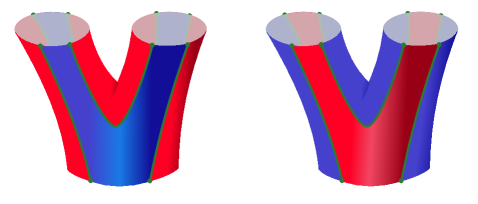
Figure 18. The two multiplications (read down) and comultiplications (read up) on $H_{1}$.

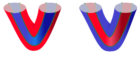
Figure 19. The two Frobenius quadratic forms, differing by the antipode

8.2.2. Relation to Hopf algebras

We determine the gauge theory space $H_{1}=\mathrsfs{Q}(D_{1,1},\partial_{c}D^{1,1})$ from the classical model of $\mathrsfs{G}_{G}$: the groupoid of bundles on $D^{1,1}$ trivialized on two arcs is equivalent to the set $G$ of monodromies, so $H_{1}$ is the space of functions on $G$. (See also Example 9.17.) This is a Hopf algebra, with two Frobenius structures for the two operations, which differ by the antipode. (The Frobenius form for the convolution algebra pairs $g$ with $g^{-1}$, while multiplication is matched with the pointwise pairing.) The Frobenius-Hopf operations have geometric interpretations, and products can be interchanged with co-products by means of the Frobenius forms, in a way that matches the switch from $H_{1}$ to its dual Hopf algebra. The geometric construction of the operations is shown in Figures 18 and 19. As the picture shows, the two Frobenius quadratic forms on $H_{1}$ do not agree, but differ by a reflection about the origin on (either) one of the factors: a quarter-rotation that identifies the two sides of Figure 19 takes opposite signs on the two input boundaries. This reflection, the $\mathrm{O}(1)$-symmetry of the handle, implements the antipode $S$. For $\mathscr{V}ect[G]$ with Dirichlet (red) and Neumann (blue) boundary structures, the left picture in Fig. 18 gives the group ring, while the right one defines the commutative multiplication on $\mathbb{C}[G]$.

This Frobenius-Hopf property is not an accident: every fusion category $\mathscr{T}$ with a fiber functor $\phi:\mathscr{T}\to\mathscr{V}ect$ is equivalent to the tensor category of modules over a finite semi-simple Hopf algebra, by a Tannakian reconstruction theorem of Hayashi [Ha] and Ostrik [Os]. Moreover, the Koszul dual category $\mathscr{E}:=\mathrm{End}_{\mathscr{T}}(\mathscr{V}ect)$ is the tensor category of co-modules; equivalently (in light of finiteness) the category of modules over the dual Hopf algebra. (The multi-fusion case is addressed by the related notion of a weak Hopf algebra, see for instance [EGNO, Ch.7].) Thus, the most general setting of our story pertains to finite, non-commutative gauge theory.

A full pictorial account of this TQFT-Hopf correspondence is planned for [FT2]; here, we merely check the requisite “Peter-Weyl” decompositions of $H_{1}$, which will ensure that we have the correct algebra in the Tannakian reconstruction theorem:

Proposition 8.9.

Let $x_{i}$ be a basis of simple objects of $\mathscr{T}$ and $y_{j}$ one for $\mathscr{E}$. Then, as algebras for the left and right multiplications in Fig. 18,

$$H_{1}\cong\bigoplus\nolimits_{i}\phi(x_{i})\otimes\phi(x_{i})^{\vee};\qquad H_{1}\cong\bigoplus\nolimits_{i}\phi(y_{i})\otimes\phi(y_{i})^{\vee}.$$

Remark 8.10.

The two identifications are related by a $\pi/4$ rotation of $\partial_{c}D^{1,1}$, which implements the Fourier transform, interchanging $\theta\leftrightarrow\theta^{\vee}$ in the duality below.

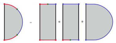
Figure 20. The fiber functor

Proof.

The interval with two red endpoints computes, under $\mathrsfs{Q}$, the category $\mathscr{T}$ (cf. Remark 6.11). We claim that the half-disk cut across the two red arcs represents the fiber functor; the theorem then follows by pre-composing this with its adjoint. The claim follows from the three-step factorization in Figure 20, which splits it into the fiber functor $\phi$ landing in $\mathscr{V}ect\simeq\mathrm{Hom}{F}(\mathrsfs{B},\mathrsfs{B}^{\prime})$; its adjoint, the inclusion of $\phi^{\vee}(\mathscr{V}ect)\subset\mathscr{E}$; and finally the application of $\mathrm{Hom}_{\mathscr{E}}(\mathbf{1},\_\,)$. Because $\phi^{\vee}(\mathbb{C})=\bigoplus_{j}y_{j}\otimes\phi(y_{j}^{\vee})$, the final two steps compose to the fiber functor. ∎

8.2.3. Order/disorder operators

Line defects in $3$D TQFT were described in §3.4, where $\mathscr{V}ect[G]$ can be replaced by a general field theory $\mathrsfs{F}$: the cited discussion converts the “line operator” language into that of bordisms with corners. We specialize to $0$- and $2$-defects. In the theory $\mathrsfs{F}_{\mathscr{T}}$ with the regular boundary condition for $\mathrsfs{B}$ and the fiber functor for $\mathrsfs{B}^{\prime}$, these are the Wilson and ’t Hooft defects; for the Hopf algebra $H_{1}$, these are the modules and co-modules, respectively. We now explain how the promotion data in Definition 8.6 leads to the defective Ising partition function (and correlators).

Repeat the cylinder construction of §8.1, with additional holes bored through $X$ at each defect. This creates a white annulus on the input face and a circular edge on the output $Y_{1}$. As we convened to insert the unit at maxima and minima, the respective defect-free disks there may be capped by colored hemispheres. We read the picture with the white annulus boundary as incoming, ready to absorb the defect label $\delta$. The other annulus boundary is colored, and the result produces the vector space $\mathrm{Hom}_{\mathscr{T}}(W_{y},\delta)$ as a new tensor factor in the domain of the map $\mathrsfs{Q}(X,Y_{c})$ in (8.2). An order operator (if $p=0$) or disorder operator ($p=2$) is a vector in the respective $\mathrm{Hom}$-space at each defect point; contracted with $\mathrsfs{Q}(X,Y_{c})$, it gives the Ising partition function in $\mathrsfs{F}(Y_{c},\vec{\delta}\,)$. This is the defective Ising partition function. A null-bordism of the defect maps it to the correlator in $\mathrsfs{F}(Y)$. The latter depends on the order/disorder insertions as well as the null-bordism of the underlying defect.

8.2.4. The Ising state space

Conversion to extended TQFT language indicates the way of factorizing Ising theories (as relative theories) on manifolds with corners. The basic rule is that any time-cut must be transversal to all structures. For instance, we can associate an object in the center category $Z(\mathscr{T})$ to any circle cutting $Y_{c}$ through red and blue faces and across the green defect lines. (We are unable to cut across the white disks, which have already absorbed a vector that does not normally factor appropriately.) When translated to the lattice, this cutting seem counter-intuitive, as it describes paths which zig-zag between vertices and face centers on the lattice: neither of the obvious cutting methods — along the edges or across the edges — is allowed, from the TQFT perspective.

The resulting circle comes subdivided into red and blue arcs. Pairing with an object in $Z(\mathscr{T})$ yields an Ising space of states. Thus, in the original Ising model, we thus get four spaces, one for each pair consisting of a holonomy in $\mbox{$\raisebox{-0.70007pt}{\rotatebox{9.0}{\tiny/}}\mu\raisebox{-4.2194pt}{\scalebox{2.0}{$\color[rgb]{1,1,1}.$}}\raisebox{3.7889pt}{$\color[rgb]{1,1,1}.$}\hskip 4.60007pt$}_{2}$ and an irreducible $\mbox{$\raisebox{-0.70007pt}{\rotatebox{9.0}{\tiny/}}\mu\raisebox{-4.2194pt}{\scalebox{2.0}{$\color[rgb]{1,1,1}.$}}\raisebox{3.7889pt}{$\color[rgb]{1,1,1}.$}\hskip 4.60007pt$}_{2}$-representation. For general $G$, we get one space for each conjugacy class and irreducible representation of the stabilizer. These spaces also have natural inner products, because of the reality and orientation-free nature of the theory. This natural inner product seems to be an advantage of the TQFT cutting over the obvious one (where correction by the square root of the action is needed). The following relies on the identification [EGNO, Proposition 7.14.6] of $Z(\mathscr{T})$ with the tensor category of modules over the Drinfeld double algebra $D(H_{1})$.

Proposition 8.11.

The Ising space of states for the circle with $N$ red/blue interval pairs is the free module $D(H_{1})\otimes H_{1}^{\otimes(n-1)}$ over the Drinfeld double, where $D(H_{1})$ acts on the first factor only.

Proof.

The space, as a module over $D(H_{1})$, is the output of $[0,1]\times S^{1}$ with the circle at $0$ subdivided into the $2N$ arcs. We compute it via the picture in Figure 21, by factoring it successively via the categories $\mathrm{Hom}(\mathrsfs{B},\mathrsfs{B}^{\prime})_{\simeq}\mathscr{V}ect$. The cutting lines for the factorization are as indicated. The first cut yields the object $\mathbb{C}$, which is then tensored with the vector space $H_{1}$ at every step. The final morphism $\mathrm{Hom}(\mathrsfs{B},\mathrsfs{B}^{\prime})\to Z(\mathscr{T})$ is the adjoint of the fiber functor on $Z(\mathscr{T})$, and produces the double $D(H_{1})$ as a module over itself, times $H_{1}^{\otimes(N-1)}$. ∎

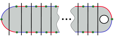
Figure 21. Computation of the Ising space of states

Remark 8.12.

This presentation breaks the cyclic ${\mathbb{Z}}/N{\mathbb{Z}}$ symmetry. A symmetric but less concrete presentation is given as follows. The center $Z(\mathscr{T})$ can be identified with the $N$-fold cyclic tensor product

$$\mathscr{T}\otimes_{\mathscr{T}}\mathscr{T}\otimes_{\mathscr{T}}\dots\otimes_{\mathscr{T}}\mathscr{T}\otimes_{\mathscr{T}}\rotatebox{90.0}{$\circlearrowleft$}$$

and receives as such an (additive) functor from $\mathscr{T}^{\otimes N}$. The Ising space of states corresponds to the image of $\chi^{\otimes N}$, where $\chi=\bigoplus_{i}x_{i}\otimes\phi(x_{i}^{\vee})$ is the image of $\mathbb{C}$ under the adjoint of the fiber functor $\phi$.

8.3. The duality theorem

The Morita equivalence between $\mathscr{T}$ and $\mathscr{E}=\mathrm{End}_{\mathscr{T}}(\mathscr{V}ect)$ interchanges their “red” and “blue” boundary conditions: $\mathscr{T}\leftrightarrow\mathscr{V}ect$ and $\mathscr{V}ect\leftrightarrow\mathscr{E}$. A matching color switch on $Y_{c}$ is realized by a change to the Morse function $d-f$, corresponding to the dual lattice. With the switch of boundary conditions comes the switch in the type of defects and (dis)order operators. We have seen above that for $\mathscr{T}=\mathscr{V}ect[G]$, the bi-colored construction reproduces the gauge theory of §3 and §7. It follows that the color switch reproduces the theory $\mathrsfs{R}_{G}$ of §7, proving, as advertised in the summary but now stated more precisely:

Theorem 8.13.

There is a natural duality, on oriented manifolds, identifying the gauge theory of a finite group $G$ with the Turaev-Viro theory based on $\mathscr{R}ep(G)$, and a matching Kramers-Wannier duality of their lattice boundary theories with Fourier dual Ising actions. There is an interchange of Wilson and ’t Hooft defects in the bulk theories, and of order and disorder operators for the boundary. Dual Ising partition match up, after adjusting an overall scale factor. ∎

Remark 8.14.

The scale factor is concealed in the choice of $\mathrm{SO}(2)$-structures for the boundary theories. The “Fourier duality” of the Ising actions is simply their transformation in the dual Hopf algebra using the Frobenius form: evenness allows us to use either of the two Frobenius pairings. Mind that both sides of the duality define unoriented theories; however, as explained in the Abelian case, the duality does require an orientation, otherwise an orientation twist is introduced.

The theorem, of course, applies to general fusion categories with a fiber functor, corresponding to finite, semi-simple Hopf algebras $H$; the categories of modules and co-modules are then interchanged. In this generalization, we leave the setting of theories quantized from a classical model of fields, but we can find new examples of self-dual theories [Ma], which is not possible in non-abelian gauge theory.

9. Higher dimensions and finite path integrals

We generalize the two-dimensional lattice model for finite abelian groups to higher dimensions. The background field encoding the higher global symmetry is a higher abelian gauge field, and the abelian case admits a natural generalization to spectra (in the sense of stable homotopy theory) which are finite homotopy types: only finitely many homotopy groups are nonzero and each is a finite group. These lattice models have arbitrary “higher groups” of this type as symmetry groups. The construction is phrased in terms of finite path integrals; see [Q, F3, Tu, FHLT] for various expositions. All spaces and spectra in this section are finite homotopy types.

9.1. Generalized finite electromagnetic duality

Suppose $S$ is a pointed space which is a finite homotopy type. The example relevant to §3 is $S=BG$ for $G$ a finite group. Fix $n\in{\mathbb{Z}}^{\geq 0}$. There is an $n$-dimensional extended topological field theory $\mathrsfs{F}_{S}$ of unoriented manifolds which counts homotopy classes of maps to $S$. Namely, if $X$ is a closed $n$-manifold, let $S^{X}=\operatorname{Map}(X,S)$ denote the space of unpointed maps from $X$ to $S$. The partition function is

(9.1) $$\mathrsfs{F}_{S}(X)=\sum\limits_{[\varphi]\in\pi_{0}S^{X}}\frac{1}{\#\pi_{1}(S^{X},\varphi)}\;\frac{\#\pi_{2}(S^{X},\varphi)}{\#\pi_{3}(S^{X},\varphi)}\cdots$$

The sum is over homotopy classes of maps $X\to S$ and $\varphi$ is a representative of a homotopy class. For $S=BG$ expression (9.1) reduces to (3.5). The weighted sum accounts for automorphisms $(\pi_{1})$, automorphisms of automorphisms $(\pi_{2})$, etc.

Example 9.2.

If $A$ is a finite abelian group and $S=B^{r}A$ is the $r^{\textnormal{th}}$ classifying space—the Eilenberg-MacLane space with $\pi_{r}S=A$—then (9.1) reduces to

(9.3) $$\mathrsfs{F}_{B^{r}A}(X)=\prod\limits_{i=0}^{r}\left(\#H^{r-i}(X;A)\right)^{(-1)^{i}}.$$

An $(n-1)$-dimensional theory relative to $\mathrsfs{F}_{B^{r}A}$ has a generalized symmetry group $B^{r-1}A$, sometimes called an “$(r-1)$-form global symmetry” [GKSW].

Remark 9.4.

We can twist the sum (9.1) by a suitable cocycle on $S$. For example, Dijkgraaf-Witten theory is the case $S=BG$ with cocycle representing a class in $H^{n}(BG;{\mathbb{R}}/2\pi i{\mathbb{Z}})$. An $(n-1)$-dimensional theory relative to it is said to have an anomalous global symmetry group $G$. Note that we can replace the mapping space $\operatorname{Map}(X_{+},BG)$—or rather its fundamental groupoid, which is all we use—by the equivalent groupoid of principal $G$-bundles over $X$. With that understood the theory of maps to $BG$ is a gauge theory. A similar remark holds for higher groups, as in Example 9.2.

Example 9.5.

Let $\mbox{$\raisebox{-0.70007pt}{\rotatebox{9.0}{\tiny/}}\mu\raisebox{-4.2194pt}{\scalebox{2.0}{$\color[rgb]{1,1,1}.$}}\raisebox{3.7889pt}{$\color[rgb]{1,1,1}.$}\hskip 4.60007pt$}_{n}\subset\mathbb{T}$ be the group of $n^{\textnormal{th}}$ roots of unity. Then there is a pointed space $S$ which fits into the (Postnikov) principal fibration

(9.6) $$B^{2}\!\mbox{$\raisebox{-0.70007pt}{\rotatebox{9.0}{\tiny/}}\mu\raisebox{-4.2194pt}{\scalebox{2.0}{$\color[rgb]{1,1,1}.$}}\raisebox{3.7889pt}{$\color[rgb]{1,1,1}.$}\hskip 4.60007pt$}_{n}\longrightarrow S\longrightarrow B\!\mbox{$\raisebox{-0.70007pt}{\rotatebox{9.0}{\tiny/}}\mu\raisebox{-4.2194pt}{\scalebox{2.0}{$\color[rgb]{1,1,1}.$}}\raisebox{3.7889pt}{$\color[rgb]{1,1,1}.$}\hskip 4.60007pt$}_{n}$$

and has $k$-invariant a generator of $H^{3}(B\!\mbox{$\raisebox{-0.70007pt}{\rotatebox{9.0}{\tiny/}}\mu\raisebox{-4.2194pt}{\scalebox{2.0}{$\color[rgb]{1,1,1}.$}}\raisebox{3.7889pt}{$\color[rgb]{1,1,1}.$}\hskip 4.60007pt$}_{n};\mbox{$\raisebox{-0.70007pt}{\rotatebox{9.0}{\tiny/}}\mu\raisebox{-4.2194pt}{\scalebox{2.0}{$\color[rgb]{1,1,1}.$}}\raisebox{3.7889pt}{$\color[rgb]{1,1,1}.$}\hskip 4.60007pt$}_{n})\cong\mbox{$\raisebox{-0.70007pt}{\rotatebox{9.0}{\tiny/}}\mu\raisebox{-4.2194pt}{\scalebox{2.0}{$\color[rgb]{1,1,1}.$}}\raisebox{3.7889pt}{$\color[rgb]{1,1,1}.$}\hskip 4.60007pt$}_{n}$. We can view $S$ as (the classifying space of) a 2-group; this 2-group acts as global symmetries on any field theory relative to $\mathrsfs{F}_{S}$. (We remark that this is a finite analog of a 2-group which acts on certain 4-dimensional gauge theories [CDI].) The $k$-invariant is unstable so this example does not extend to a spectrum. Still, it is possible that there is an electromagnetic dual.

The finite path integral constructs an extended $n$-dimensional topological field theory: a vector space for a closed $(n-1)$-manifold, a linear category or algebra for a closed $(n-2)$-manifold, etc. See [F3] for a heuristic treatment, [FHLT, §3] for examples, and [FHLT, §8] for a general discussion. Here we are content to tell the result of the finite path integral in codimensions one and two.

Let $Y$ be a closed $(n-1)$-manifold. The vector space $\mathrsfs{F}_{S}(Y)$ is simply $\operatorname{Fun}(\pi_{0}S^{Y})$, the space of functions on the set $[Y_{+},S]$ of (free) homotopy classes of maps $Y\to S$. If we twist by a cocycle representing a class $\alpha\in H^{n}(S;{\mathbb{R}}/2\pi i{\mathbb{Z}})$, as in Remark 9.4, then for $Y$ oriented we construct a line bundle $p\colon\mathscr{L}\to\pi_{\leq 1}S^{Y}$ over the fundamental groupoid of $\operatorname{Map}(Y_{+}S)$. (See [FQ, Appendix B] for a special case.) Then $\mathrsfs{F}_{S}(Y)$ is the vector space of sections of $p$. Observe that a loop in $\pi_{\leq 1}S^{Y}$—an automorphism of a map $\varphi\colon Y\to S$—is a map $f\colon S^{1}\times Y\to S$. The holonomy of $\mathscr{L}\to\pi_{\leq 1}S^{Y}$ around the loop is $\exp(\langle f^{*}\alpha,[S^{1}\times Y]\rangle)\in\mathbb{T}$. If it is nontrivial for any loop based at $\varphi$, then all sections of $p$ vanish at $\varphi$.

To a closed $(n-2)$-manifold $Z$ we attach the linear category $\mathrsfs{F}_{S}(Z)$ of complex vector bundles over $\pi_{\leq 1}S^{Z}$, the fundamental groupoid of the space of maps $Z\to S$. This is the category of representations of the path algebra of a finite groupoid equivalent to $\pi_{\leq 1}S^{Z}$. In the presence of a nonzero cocycle we obtain a category of twisted vector bundles, or equivalently the category of representations of a twisted path algebra; see [F3, §8] for an example.

Now suppose that $S$ has an infinite loop space structure, i.e., a choice of spaces $T_{m}$, $m\in{\mathbb{Z}}^{\geq 0}$, and homotopy equivalences $S\to\Omega^{m}T_{m}$ which exhibit $S$ as an $m$-fold loop space for every $m\in{\mathbb{Z}}^{\geq 0}$. Equivalently, a sequence $\{T_{m}\}_{m\in{\mathbb{Z}}^{\geq 0}}$ of pointed spaces and homotopy equivalences $T_{m}\to\Omega T_{m+1}$ defines a spectrum $\boldsymbol{T}$ and exhibits $S=T_{0}$ as the 0-space of the spectrum. For example, $S=B^{r}A$ is the 0-space of the shifted Eilenberg-MacLane spectrum $\Sigma^{r}HA$. Spectra give homology and cohomology theories, and vice versa; we write $H_{\bullet}(X;\boldsymbol{T})$, $H^{\bullet}(X;\boldsymbol{T})$ for the homology, respectively cohomology, of a space $X$ with coefficients in the spectrum $\boldsymbol{T}$. A spectrum $\boldsymbol{T}$ has a character dual spectrum $\boldsymbol{T}^{\vee}$ defined as the cohomology theory

(9.7) $$H^{q}(X;\boldsymbol{T}^{\vee}):=\operatorname{Hom}\bigl{(}H_{q}(X;\boldsymbol{T}),\mathbb{T}\bigr{)}=H_{q}(X;\boldsymbol{T})^{\vee}.$$

The dual to the sphere spectrum is denoted $I\mathbb{T}$, and then $\boldsymbol{T}^{\vee}=\operatorname{Map}(\boldsymbol{T},I\mathbb{T})$. Take $X=\operatorname{pt}$ in (9.7) to conclude that the homotopy groups of $\boldsymbol{T}^{\vee}$ are the Pontrjagin duals to the homotopy groups of $\boldsymbol{T}$:

(9.8) $$\pi_{q}\boldsymbol{T}^{\vee}\cong\left(\pi_{-q}\boldsymbol{T}\right)^{\vee},\qquad q\in{\mathbb{Z}}.$$

$\boldsymbol{T}^{\vee}$ has finite homotopy type if and only if $\boldsymbol{T}$ does.

Definition 9.9.

Let $\mathrsfs{F}_{\boldsymbol{T}}\colon\operatorname{Bord}_{n}\to\mathscr{C}$ be the finite path integral theory based on the spectrum $\boldsymbol{T}$. The electromagnetic dual theory $(\mathrsfs{F}_{\boldsymbol{T}})^{\vee}=\mathrsfs{F}_{\Sigma^{n-1}\boldsymbol{T}^{\vee}}$ is the finite path integral theory based on the shifted character dual spectrum $\Sigma^{n-1}\boldsymbol{T}^{\vee}$.

The abelian duality of §3.3 is the case $n=3$, $\boldsymbol{T}=\Sigma HA$, for a finite abelian group $A$. The correspondence diagram (3.30) of pointed spaces, which expresses the duality, generalizes to arbitrary spectra as the commutative diagram of spectra

(9.10) $$\begin{gathered}\lx@xy@svg{\hbox{\raise 0.0pt\hbox{\kern 6.61632pt\hbox{\ignorespaces\ignorespaces\ignorespaces\hbox{\vtop{\kern 0.0pt\offinterlineskip\halign{\entry@#!@&&\entry@@#!@\cr&\\&&\crcr}}}\ignorespaces{\hbox{\kern-3.0pt\raise 0.0pt\hbox{\hbox{\kern 0.0pt\raise 0.0pt\hbox{\hbox{\kern 3.0pt\raise 0.0pt\hbox{$\textstyle{}$}}}}}}}{\hbox{\kern 30.61632pt\raise 0.0pt\hbox{\hbox{\kern 0.0pt\raise 0.0pt\hbox{\hbox{\kern 3.0pt\raise 0.0pt\hbox{$\textstyle{(\boldsymbol{T}\times\Sigma^{n-1}\boldsymbol{T}^{\vee},c)\ignorespaces\ignorespaces\ignorespaces\ignorespaces\ignorespaces\ignorespaces\ignorespaces\ignorespaces}$}}}}}}}\ignorespaces\ignorespaces\ignorespaces{}\ignorespaces\ignorespaces{\hbox{\lx@xy@drawline@}}\ignorespaces\ignorespaces\ignorespaces{\hbox{\kern 24.062pt\raise-14.75638pt\hbox{{}\hbox{\kern 0.0pt\raise 0.0pt\hbox{\hbox{\kern 3.0pt\hbox{\hbox{\kern 0.0pt\raise-0.8264pt\hbox{$\scriptstyle{p}$}}}\kern 3.0pt}}}}}}\ignorespaces{\hbox{\kern 6.61633pt\raise-35.73964pt\hbox{\hbox{\kern 0.0pt\raise 0.0pt\hbox{\lx@xy@tip{1}\lx@xy@tip{-1}}}}}}\ignorespaces\ignorespaces{\hbox{\lx@xy@drawline@}}\ignorespaces{\hbox{\lx@xy@drawline@}}\ignorespaces\ignorespaces\ignorespaces{}\ignorespaces\ignorespaces{\hbox{\lx@xy@drawline@}}\ignorespaces\ignorespaces\ignorespaces{\hbox{\kern 98.0359pt\raise-14.75638pt\hbox{{}\hbox{\kern 0.0pt\raise 0.0pt\hbox{\hbox{\kern 3.0pt\hbox{\hbox{\kern 0.0pt\raise-0.8264pt\hbox{$\scriptstyle{q}$}}}\kern 3.0pt}}}}}}\ignorespaces{\hbox{\kern 120.61491pt\raise-31.1101pt\hbox{\hbox{\kern 0.0pt\raise 0.0pt\hbox{\lx@xy@tip{1}\lx@xy@tip{-1}}}}}}\ignorespaces\ignorespaces{\hbox{\lx@xy@drawline@}}\ignorespaces{\hbox{\lx@xy@drawline@}}{\hbox{\kern-6.61632pt\raise-39.88776pt\hbox{\hbox{\kern 0.0pt\raise 0.0pt\hbox{\hbox{\kern 3.0pt\raise 0.0pt\hbox{$\textstyle{\boldsymbol{T}}$}}}}}}}{\hbox{\kern 60.61562pt\raise-39.88776pt\hbox{\hbox{\kern 0.0pt\raise 0.0pt\hbox{\hbox{\kern 3.0pt\raise 0.0pt\hbox{$\textstyle{}$}}}}}}}{\hbox{\kern 120.61491pt\raise-39.88776pt\hbox{\hbox{\kern 0.0pt\raise 0.0pt\hbox{\hbox{\kern 3.0pt\raise 0.0pt\hbox{$\textstyle{\Sigma^{n-1}\boldsymbol{T}^{\vee}}$}}}}}}}\ignorespaces}}}}\ignorespaces\end{gathered} \textstyle{(\boldsymbol{T}\times\Sigma^{n-1}\boldsymbol{T}^{\vee},c)\ignorespaces\ignorespaces\ignorespaces\ignorespaces\ignorespaces\ignorespaces\ignorespaces\ignorespaces} \scriptstyle{p} \scriptstyle{q} \textstyle{\boldsymbol{T}} \textstyle{\Sigma^{n-1}\boldsymbol{T}^{\vee}} \textstyle{(\boldsymbol{T}\times\Sigma^{n-1}\boldsymbol{T}^{\vee},c)\ignorespaces\ignorespaces\ignorespaces\ignorespaces\ignorespaces\ignorespaces\ignorespaces\ignorespaces} \scriptstyle{p} \scriptstyle{q} \textstyle{\boldsymbol{T}} \textstyle{\Sigma^{n-1}\boldsymbol{T}^{\vee}}$$

in which

(9.11) $$c\colon\boldsymbol{T}\times\Sigma^{n-1}\boldsymbol{T}^{\vee}\longrightarrow\Sigma^{n-1}I\mathbb{T}$$

is the canonical duality map, which here represents an $(n-1)$-dimensional domain wall. Let $T_{0}$ be the 0-space of $\boldsymbol{T}$ and $T_{n-1}^{\vee}$ the 0-space of $\Sigma^{n-1}\boldsymbol{T}^{\vee}$. Then if $X=X^{\prime}\cup_{Y}X^{\prime\prime}$ is an $n$-manifold decomposed into the union of submanifolds $X^{\prime},X^{\prime\prime}$ with boundary intersecting in the $(n-1)$-dimensional submanifold $Y$, a field in the theory with domain wall is a pair $(\varphi^{\prime},\varphi^{\prime\prime})$ of maps $\varphi^{\prime}\colon X^{\prime}\to T_{0}$ and $\varphi^{\prime\prime}\colon X^{\prime\prime}\to T_{n-1}^{\vee}$. On the restriction to $Y$ we obtain a representative of a class in $H^{n-1}(Y;I\mathbb{T})$. As in §3.3 we can use it to define a Fourier transform between the vector spaces associated to $Y$ in the theories $\mathrsfs{F}_{\boldsymbol{T}}$ and $(\mathrsfs{F}_{\boldsymbol{T}})^{\vee}$.

Remark 9.12.

At first glance to integrate this class over $Y$ requires a framing on $Y$, since the cohomology theory $I\mathbb{T}$ is oriented for framed manifolds. But the duality map (9.11) may factor through a simpler cohomology theory with a less stringent orientation condition. For example, the duality map in (3.30) takes values in $H\mathbb{T}$, so can be integrated over (standardly) oriented manifolds.

Remark 9.13.

In the simplest case, $\boldsymbol{T}=\Sigma^{r}HA$ is the shifted Eilenberg-MacLane spectrum of a finite abelian group $A$. Then $\varphi\colon X\to T_{0}$ represents a class in $H^{r}(X;A)$. Electromagnetic duality is well-known for such higher abelian gauge fields.

9.2. Boundary theories and domain walls

Let $S,B$ be pointed spaces, both finite homotopy types, and suppose $\pi\colon B\to S$ is a fibration. From this data we construct a boundary theory $\mathrsfs{B}_{B}$ for $\mathrsfs{F}_{S}$. A field on a manifold $X$ with boundary is $\varphi\colon X\to S$ as before, together with a lift $\psi\colon\partial X\to B$ of the restriction of $\varphi$ to $\partial X$. So, for example, the value of $\mathrsfs{B}_{B}$ on a closed $(n-1)$-manifold $Y$ is the function of the field $\varphi\colon Y\to S$ defined by counting lifts $\psi\colon Y\to B$ of $\varphi$ up to homotopy. Let $B^{Y}\!/\varphi$ denote the space of lifts. Then we have

(9.14) $$(\mathrsfs{F}_{S},\mathrsfs{B}_{B})(Y)(\varphi)=\sum\limits_{[\psi]\in\pi_{0}B^{Y}\!/\varphi}\frac{1}{\#\pi_{1}(B^{Y}\!/\varphi,\psi)}\;\frac{\#\pi_{2}(B^{Y}\!/\varphi,\psi)}{\#\pi_{3}(B^{Y}\!/\varphi,\psi)}\cdots,$$

where we sum over homotopy classes of lifts. The result only depends on the homotopy class of $\varphi$.

For any $S$ there are two canonical boundary theories. The first is associated to the inclusion $*\to S$ of the basepoint, made into a fibration by replacing $*$ with the contractible space $P(S)$ of paths $\gamma\colon[0,1]\to S$ with $\gamma(0)=*$. We call this the Dirichlet boundary theory. The second is associated to the identity map $S\to S$ and is termed the Neumann boundary theory. For finite gauge theory $S=BG$ the field $\varphi$ may be replaced by a principal $G$-bundle (Remark 9.4), in which case the Dirichlet boundary field is a trivialization of the $G$-bundle and, as in general, the Neumann boundary field is trivial. These boundary theories are denoted $\mathrsfs{B}_{e}$ and $\mathrsfs{B}_{G}$, respectively, in (3.9).

If pointed spaces $S_{1},S_{2}$ of finite homotopy type define theories $\mathrsfs{F}_{S_{1}},\mathrsfs{F}_{S_{2}}$, then a correspondence diagram

(9.15) $$\begin{gathered}\lx@xy@svg{\hbox{\raise 0.0pt\hbox{\kern 7.75415pt\hbox{\ignorespaces\ignorespaces\ignorespaces\hbox{\vtop{\kern 0.0pt\offinterlineskip\halign{\entry@#!@&&\entry@@#!@\cr&\\&&\crcr}}}\ignorespaces{\hbox{\kern-3.0pt\raise 0.0pt\hbox{\hbox{\kern 0.0pt\raise 0.0pt\hbox{\hbox{\kern 3.0pt\raise 0.0pt\hbox{$\textstyle{}$}}}}}}}{\hbox{\kern 31.75415pt\raise 0.0pt\hbox{\hbox{\kern 0.0pt\raise 0.0pt\hbox{\hbox{\kern 3.0pt\raise 0.0pt\hbox{$\textstyle{D\ignorespaces\ignorespaces\ignorespaces\ignorespaces\ignorespaces\ignorespaces\ignorespaces\ignorespaces}$}}}}}}}\ignorespaces\ignorespaces\ignorespaces{}\ignorespaces\ignorespaces{\hbox{\lx@xy@drawline@}}\ignorespaces{\hbox{\kern 7.75417pt\raise-30.23885pt\hbox{\hbox{\kern 0.0pt\raise 0.0pt\hbox{\lx@xy@tip{1}\lx@xy@tip{-1}}}}}}\ignorespaces\ignorespaces{\hbox{\lx@xy@drawline@}}\ignorespaces{\hbox{\lx@xy@drawline@}}\ignorespaces\ignorespaces\ignorespaces{}\ignorespaces\ignorespaces{\hbox{\lx@xy@drawline@}}\ignorespaces{\hbox{\kern 70.3111pt\raise-30.24643pt\hbox{\hbox{\kern 0.0pt\raise 0.0pt\hbox{\lx@xy@tip{1}\lx@xy@tip{-1}}}}}}\ignorespaces\ignorespaces{\hbox{\lx@xy@drawline@}}\ignorespaces{\hbox{\lx@xy@drawline@}}{\hbox{\kern-7.75415pt\raise-37.73553pt\hbox{\hbox{\kern 0.0pt\raise 0.0pt\hbox{\hbox{\kern 3.0pt\raise 0.0pt\hbox{$\textstyle{S_{1}}$}}}}}}}{\hbox{\kern 36.03262pt\raise-37.73553pt\hbox{\hbox{\kern 0.0pt\raise 0.0pt\hbox{\hbox{\kern 3.0pt\raise 0.0pt\hbox{$\textstyle{}$}}}}}}}{\hbox{\kern 70.3111pt\raise-37.73553pt\hbox{\hbox{\kern 0.0pt\raise 0.0pt\hbox{\hbox{\kern 3.0pt\raise 0.0pt\hbox{$\textstyle{S_{2}}$}}}}}}}\ignorespaces}}}}\ignorespaces\end{gathered} \textstyle{D\ignorespaces\ignorespaces\ignorespaces\ignorespaces\ignorespaces\ignorespaces\ignorespaces\ignorespaces} \textstyle{S_{1}} \textstyle{S_{2}} \textstyle{D\ignorespaces\ignorespaces\ignorespaces\ignorespaces\ignorespaces\ignorespaces\ignorespaces\ignorespaces} \textstyle{S_{1}} \textstyle{S_{2}}$$

of finite homotopy type pointed spaces defines a domain wall $\mathrsfs{D}_{D}\colon\mathrsfs{F}_{S_{1}}\to\mathrsfs{F}_{S_{2}}$. Similarly, a commutative diagram

(9.16) $$\begin{gathered}\lx@xy@svg{\hbox{\raise 0.0pt\hbox{\kern 7.0434pt\hbox{\ignorespaces\ignorespaces\ignorespaces\hbox{\vtop{\kern 0.0pt\offinterlineskip\halign{\entry@#!@&&\entry@@#!@\cr&\\&&\\&\crcr}}}\ignorespaces{\hbox{\kern-3.0pt\raise 0.0pt\hbox{\hbox{\kern 0.0pt\raise 0.0pt\hbox{\hbox{\kern 3.0pt\raise 0.0pt\hbox{$\textstyle{}$}}}}}}}{\hbox{\kern 31.0434pt\raise 0.0pt\hbox{\hbox{\kern 0.0pt\raise 0.0pt\hbox{\hbox{\kern 3.0pt\raise 0.0pt\hbox{$\textstyle{D\ignorespaces\ignorespaces\ignorespaces\ignorespaces\ignorespaces\ignorespaces\ignorespaces\ignorespaces}$}}}}}}}\ignorespaces\ignorespaces\ignorespaces{}\ignorespaces\ignorespaces{\hbox{\lx@xy@drawline@}}\ignorespaces{\hbox{\kern 7.04341pt\raise-30.69836pt\hbox{\hbox{\kern 0.0pt\raise 0.0pt\hbox{\lx@xy@tip{1}\lx@xy@tip{-1}}}}}}\ignorespaces\ignorespaces{\hbox{\lx@xy@drawline@}}\ignorespaces{\hbox{\lx@xy@drawline@}}\ignorespaces\ignorespaces\ignorespaces{}\ignorespaces\ignorespaces{\hbox{\lx@xy@drawline@}}\ignorespaces{\hbox{\kern 69.60034pt\raise-30.1029pt\hbox{\hbox{\kern 0.0pt\raise 0.0pt\hbox{\lx@xy@tip{1}\lx@xy@tip{-1}}}}}}\ignorespaces\ignorespaces{\hbox{\lx@xy@drawline@}}\ignorespaces{\hbox{\lx@xy@drawline@}}{\hbox{\kern-7.0434pt\raise-37.61108pt\hbox{\hbox{\kern 0.0pt\raise 0.0pt\hbox{\hbox{\kern 3.0pt\raise 0.0pt\hbox{$\textstyle{B\ignorespaces\ignorespaces\ignorespaces\ignorespaces}$}}}}}}}\ignorespaces\ignorespaces\ignorespaces{}\ignorespaces\ignorespaces{\hbox{\lx@xy@drawline@}}\ignorespaces{\hbox{\kern 31.96771pt\raise-68.99213pt\hbox{\hbox{\kern 0.0pt\raise 0.0pt\hbox{\lx@xy@tip{1}\lx@xy@tip{-1}}}}}}\ignorespaces\ignorespaces{\hbox{\lx@xy@drawline@}}\ignorespaces{\hbox{\lx@xy@drawline@}}{\hbox{\kern 35.32187pt\raise-37.61108pt\hbox{\hbox{\kern 0.0pt\raise 0.0pt\hbox{\hbox{\kern 3.0pt\raise 0.0pt\hbox{$\textstyle{}$}}}}}}}{\hbox{\kern 69.60034pt\raise-37.61108pt\hbox{\hbox{\kern 0.0pt\raise 0.0pt\hbox{\hbox{\kern 3.0pt\raise 0.0pt\hbox{$\textstyle{B^{\prime}\ignorespaces\ignorespaces\ignorespaces\ignorespaces}$}}}}}}}\ignorespaces\ignorespaces\ignorespaces{}\ignorespaces\ignorespaces{\hbox{\lx@xy@drawline@}}\ignorespaces{\hbox{\kern 44.67603pt\raise-69.11002pt\hbox{\hbox{\kern 0.0pt\raise 0.0pt\hbox{\lx@xy@tip{1}\lx@xy@tip{-1}}}}}}\ignorespaces\ignorespaces{\hbox{\lx@xy@drawline@}}\ignorespaces{\hbox{\lx@xy@drawline@}}{\hbox{\kern-3.0pt\raise-75.22217pt\hbox{\hbox{\kern 0.0pt\raise 0.0pt\hbox{\hbox{\kern 3.0pt\raise 0.0pt\hbox{$\textstyle{}$}}}}}}}{\hbox{\kern 31.96771pt\raise-75.22217pt\hbox{\hbox{\kern 0.0pt\raise 0.0pt\hbox{\hbox{\kern 3.0pt\raise 0.0pt\hbox{$\textstyle{S}$}}}}}}}\ignorespaces}}}}\ignorespaces\end{gathered} \textstyle{D\ignorespaces\ignorespaces\ignorespaces\ignorespaces\ignorespaces\ignorespaces\ignorespaces\ignorespaces} \textstyle{B\ignorespaces\ignorespaces\ignorespaces\ignorespaces} \textstyle{B^{\prime}\ignorespaces\ignorespaces\ignorespaces\ignorespaces} \textstyle{S} \textstyle{D\ignorespaces\ignorespaces\ignorespaces\ignorespaces\ignorespaces\ignorespaces\ignorespaces\ignorespaces} \textstyle{B\ignorespaces\ignorespaces\ignorespaces\ignorespaces} \textstyle{B^{\prime}\ignorespaces\ignorespaces\ignorespaces\ignorespaces} \textstyle{S}$$

determines a domain wall between the boundary theories $\mathrsfs{B}_{B}\mathrsfs{B}_{B^{\prime}}$. There is a canonical domain wall between the Dirichlet and Neumann boundary theories for any $S$.

Example 9.17.

Fix $n=3$ and $S=BG$ for $G$ a finite group. We use the canonical Dirichlet (red) and Neumann (blue) boundary theories and the canonical domain wall (green) between them. Let $Y$ be a closed 2-manifold. Then $\mathrsfs{F}_{S}(Y)$ is the space of functions on $\operatorname{Bun}_{G}(Y)$, as in (3.6). If we “color” $Y$ red, so evaluate the pair $(\mathrsfs{F}_{BG},\mathrsfs{B}_{\textnormal{Dirichlet}})$ on $Y$, we obtain a vector in $\mathrsfs{F}_{S}(Y)$—a function on $\operatorname{Bun}_{G}(Y)$—by counting trivializations: the value of this function on a principal $G$-bundle $Q\to Y$ is zero if $Q\to Y$ is not trivializable and is $(\#G)^{\#\pi_{0}Y}$ if it is trivializable. If instead we color $Y$ blue, then we deduce that $(\mathrsfs{F}_{BG},\mathrsfs{B}_{\textnormal{Neumann}})(Y)$ is the constant function with value 1.

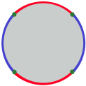
Figure 22. A 2-disk with colored boundary

For more exercise we evaluate the quartet $(\mathrsfs{F}_{BG},\mathrsfs{B}_{\textnormal{Dirichlet}},\mathrsfs{B}_{\textnormal{Neumann}},\mathrsfs{D}_{\textnormal{canonical}})$ on the 2-dimensional disk $Y$ which is pictured in Figure 22. The boundary is divided into two sets of alternating blue and red intervals connected by a total of 4 green points. The quartet is associated to the diagram

(9.18) $$\begin{gathered}\lx@xy@svg{\hbox{\raise 0.0pt\hbox{\kern 9.25pt\hbox{\ignorespaces\ignorespaces\ignorespaces\hbox{\vtop{\kern 0.0pt\offinterlineskip\halign{\entry@#!@&&\entry@@#!@\cr&\\&&\\&\crcr}}}\ignorespaces{\hbox{\kern-3.0pt\raise 0.0pt\hbox{\hbox{\kern 0.0pt\raise 0.0pt\hbox{\hbox{\kern 3.0pt\raise 0.0pt\hbox{$\textstyle{}$}}}}}}}{\hbox{\kern 34.97464pt\raise 0.0pt\hbox{\hbox{\kern 0.0pt\raise 0.0pt\hbox{\hbox{\kern 3.0pt\raise 0.0pt\hbox{$\textstyle{\**\ignorespaces\ignorespaces\ignorespaces\ignorespaces\ignorespaces\ignorespaces\ignorespaces\ignorespaces}$}}}}}}}\ignorespaces\ignorespaces\ignorespaces{}\ignorespaces\ignorespaces{\hbox{\lx@xy@drawline@}}\ignorespaces{\hbox{\kern 9.25002pt\raise-30.84302pt\hbox{\hbox{\kern 0.0pt\raise 0.0pt\hbox{\lx@xy@tip{1}\lx@xy@tip{-1}}}}}}\ignorespaces\ignorespaces{\hbox{\lx@xy@drawline@}}\ignorespaces{\hbox{\lx@xy@drawline@}}\ignorespaces\ignorespaces\ignorespaces{}\ignorespaces\ignorespaces{\hbox{\lx@xy@drawline@}}\ignorespaces{\hbox{\kern 79.19928pt\raise-29.69728pt\hbox{\hbox{\kern 0.0pt\raise 0.0pt\hbox{\lx@xy@tip{1}\lx@xy@tip{-1}}}}}}\ignorespaces\ignorespaces{\hbox{\lx@xy@drawline@}}\ignorespaces{\hbox{\lx@xy@drawline@}}{\hbox{\kern-9.25pt\raise-39.0pt\hbox{\hbox{\kern 0.0pt\raise 0.0pt\hbox{\hbox{\kern 3.0pt\raise 0.0pt\hbox{$\textstyle{\**\ignorespaces\ignorespaces\ignorespaces\ignorespaces}$}}}}}}}\ignorespaces\ignorespaces\ignorespaces{}\ignorespaces\ignorespaces{\hbox{\lx@xy@drawline@}}\ignorespaces{\hbox{\kern 33.25pt\raise-67.51749pt\hbox{\hbox{\kern 0.0pt\raise 0.0pt\hbox{\lx@xy@tip{1}\lx@xy@tip{-1}}}}}}\ignorespaces\ignorespaces{\hbox{\lx@xy@drawline@}}\ignorespaces{\hbox{\lx@xy@drawline@}}{\hbox{\kern 41.22464pt\raise-39.0pt\hbox{\hbox{\kern 0.0pt\raise 0.0pt\hbox{\hbox{\kern 3.0pt\raise 0.0pt\hbox{$\textstyle{}$}}}}}}}{\hbox{\kern 79.19928pt\raise-39.0pt\hbox{\hbox{\kern 0.0pt\raise 0.0pt\hbox{\hbox{\kern 3.0pt\raise 0.0pt\hbox{$\textstyle{BG\ignorespaces\ignorespaces\ignorespaces\ignorespaces}$}}}}}}}\ignorespaces\ignorespaces\ignorespaces{}\ignorespaces\ignorespaces{\hbox{\lx@xy@drawline@}}\ignorespaces{\hbox{\kern 55.1993pt\raise-67.86043pt\hbox{\hbox{\kern 0.0pt\raise 0.0pt\hbox{\lx@xy@tip{1}\lx@xy@tip{-1}}}}}}\ignorespaces\ignorespaces{\hbox{\lx@xy@drawline@}}\ignorespaces{\hbox{\lx@xy@drawline@}}{\hbox{\kern-3.0pt\raise-76.91666pt\hbox{\hbox{\kern 0.0pt\raise 0.0pt\hbox{\hbox{\kern 3.0pt\raise 0.0pt\hbox{$\textstyle{}$}}}}}}}{\hbox{\kern 33.25pt\raise-76.91666pt\hbox{\hbox{\kern 0.0pt\raise 0.0pt\hbox{\hbox{\kern 3.0pt\raise 0.0pt\hbox{$\textstyle{BG}$}}}}}}}\ignorespaces}}}}\ignorespaces\end{gathered} \textstyle{\**\ignorespaces\ignorespaces\ignorespaces\ignorespaces\ignorespaces\ignorespaces\ignorespaces\ignorespaces} \textstyle{\**\ignorespaces\ignorespaces\ignorespaces\ignorespaces} \textstyle{BG\ignorespaces\ignorespaces\ignorespaces\ignorespaces} \textstyle{BG} \textstyle{\**\ignorespaces\ignorespaces\ignorespaces\ignorespaces\ignorespaces\ignorespaces\ignorespaces\ignorespaces} \textstyle{\**\ignorespaces\ignorespaces\ignorespaces\ignorespaces} \textstyle{BG\ignorespaces\ignorespaces\ignorespaces\ignorespaces} \textstyle{BG}$$

The value of the quartet on $Y$ is a vector space, as it is for a closed uncolored surface. The finite path integral description tells that it is the vector space of functions on path components of fields on $Y$, which are $G$-bundles trivialized over the red and green portions of the boundary. The result is isomorphic to the space of functions on $G$. This is used in §8.2.

For any finite homotopy type $S$, the Dirichlet and Neumann boundary theories, together with the canonical domain wall between them, can be input to the constructions of §8 to yield lattice theories.

References

- [At] M. Atiyah, Topological quantum field theories, Inst. Hautes Études Sci. Publ. Math. (1988), no. 68, 175–186 (1989).
- [BC] E. H. Brown and M. Comenetz, Pontrjagin duality for generalized homology and cohomology theories, Amer. J. Math. 98 (1976), 1–27.
- [BD] John C. Baez and James Dolan, Higher-dimensional algebra and topological quantum field theory, J. Math. Phys. 36 (1995), no. 11, 6073–6105, arXiv:q-alg/950300.
- [BFN] David Ben-Zvi, John Francis, and David Nadler, Integral transforms and Drinfeld centers in derived algebraic geometry, J. Amer. Math. Soc. 23 (2010), no. 4, 909–966, arXiv:0805.0157.
- [BG] David Ben-Zvi and Sam Gunningham, Symmetries of categorical representations and the quantum Ngô action, arXiv:1712.01963.
- [BK] Benjamin Balsam and Alexander Kirillov Jr., Turaev-Viro invariants as an extended TQFT, arXiv:1004.1533.
- [BW1] John W. Barrett and Bruce W. Westbury, Spherical categories, Adv. Math. 143 (1999), no. 2, 357–375, arXiv:hep-th/9310164.
- [BW2] by same author, Invariants of piecewise-linear -manifolds, Trans. Amer. Math. Soc. 348 (1996), no. 10, 3997–4022.
- [C] John Cardy, Scaling and renormalization in statistical physics, Cambridge Lecture Notes in Physics, vol. 5, Cambridge University Press, Cambridge, 1996.
- [CDI] Clay Cordova, Thomas T. Dumitrescu, and Kenneth Intriligator, Exploring 2-group global symmetries, arXiv:1802.04790.
- [D] A. Debray. in preparation.
- [Da] O. Davidovich, State sums in -dimensional fully extended topological field theories, Ph.D. thesis, University of Texas at Austin, 2011. http://repositories.lib.utexas.edu/handle/2152/ETD-UT-2011-05-3139.
- [DSPS] Christopher L. Douglas, Christopher Schommer-Pries, and Noah Snyder, Dualizable tensor categories, arXiv:1312.7188.
- [EGNO] Pavel Etingof, Shlomo Gelaki, Dmitri Nikshych, and Victor Ostrik, Tensor categories, Mathematical Surveys and Monographs, vol. 205, American Mathematical Society, Providence, RI, 2015.
- [F1] Daniel S. Freed, The cobordism hypothesis, Bull. Amer. Math. Soc. (N.S.) 50 (2013), no. 1, 57–92, arXiv:1210.5100.
- [F2] D. S. Freed, CBMS lectures, 2017. in preparation.
- [F3] Daniel S. Freed, Higher algebraic structures and quantization, Comm. Math. Phys. 159 (1994), no. 2, 343–398, arXiv:hep-th/9212115.
- [FH] D. S. Freed and M. J. Hopkins, Reflection positivity and invertible topological phases, arXiv:1604.06527.
- [FHLT] Daniel S. Freed, Michael J. Hopkins, Jacob Lurie, and Constantin Teleman, Topological quantum field theories from compact Lie groups, A celebration of the mathematical legacy of Raoul Bott, CRM Proc. Lecture Notes, vol. 50, Amer. Math. Soc., Providence, RI, 2010, pp. 367–403. arXiv:0905.0731.
- [FHT] D. S. Freed, M. J. Hopkins, and C. Teleman, Loop groups and twisted -theory I, J. Topology 4 (2011), 737–798, arXiv:0711.1906.
- [FQ] Daniel S. Freed and Frank Quinn, Chern-Simons theory with finite gauge group, Comm. Math. Phys. 156 (1993), no. 3, 435–472, arXiv:hep-th/911100.
- [FT1] Daniel S. Freed and Constantin Teleman, Relative quantum field theory, Comm. Math. Phys. 326 (2014), no. 2, 459–476, arXiv:1212.1692.
- [FT2] D. S. Freed and C. Teleman. in preparation.
- [GKSW] Davide Gaiotto, Anton Kapustin, Nathan Seiberg, and Brian Willett, Generalized global symmetries, J. High Energy Phys. (2015), no. 2, 172, front matter+61, arXiv:1412.5148.
- [Ha] Takahiro Hayashi, A canonical Tannaka duality for finite seimisimple tensor categories, arXiv:math/9904073.
- [ID] Claude Itzykson and Jean-Michel Drouffe, Statistical field theory. Vol. 1, Cambridge Monographs on Mathematical Physics, Cambridge University Press, Cambridge, 1989. From Brownian motion to renormalization and lattice gauge theory.
- [JFS] Theo Johnson-Freyd and Claudia Scheimbauer, (Op)lax natural transformations, twisted quantum field theories, and “even higher” Morita categories, Adv. Math. 307 (2017), 147–223, arXiv:1502.06526.
- [KS] Anton Kapustin and Nathan Seiberg, Coupling a QFT to a TQFT and Duality, Journal of High Energy Physics 2014 (2014), no. 4, 1, arXiv:1401.0740.
- [L] Jacob Lurie, On the classification of topological field theories, Current developments in mathematics, 2008, Int. Press, Somerville, MA, 2009, pp. 129–280. arXiv:0905.0465.
- [La] C. I. Lazaroiu, On the structure of open-closed topological field theory in two dimensions, Nuclear Phys. B 603 (2001), no. 3, 497–530, hep-th/0010269.
- [LR] Richard G. Larson and David E. Radford, Finite-dimensional cosemisimple Hopf algebras in characteristic are semisimple, J. Algebra 117 (1988), no. 2, 267–289.
- [Ma] Akira Masuoka, Classification of semisimple Hopf algebras, Handbook of algebra. Vol. 5, Handb. Algebr., vol. 5, Elsevier/North-Holland, Amsterdam, 2008, pp. 429–455.
- [MS] G. W. Moore and G. B. Segal, D-branes and -theory in 2D topological field theory, Dirichlet branes and mirror symmetry (Paul S. Aspinwall, Tom Bridgeland, Alastair Craw, Michael R. Douglas, Mark Gross, Anton Kapustin, Gregory W. Moore, Graeme Segal, Balázs Szendrői, and P. M. H. Wilson, eds.), Clay Mathematics Monographs, vol. 4, American Mathematical Society, Providence, RI, 2009, pp. x+681. arXiv:hep-th/0609042.
- [O] Lars Onsager, Crystal statistics. I. A two-dimensional model with an order-disorder transition, Physical Review 65 (1944), no. 3-4, 117.
- [Os] Victor Ostrik, Module categories, weak Hopf algebras and modular invariants, Transform. Groups 8 (2003), no. 2, 177–206.
- [P] Rudolf Peierls, On Ising’s model of ferromagnetism, Mathematical Proceedings of the Cambridge Philosophical Society, vol. 32, Cambridge University Press, 1936, pp. 477–481.
- [Q] Frank Quinn, Lectures on axiomatic topological quantum field theory, Geometry and quantum field theory (Park City, UT, 1991), IAS/Park City Math. Ser., vol. 1, Amer. Math. Soc., Providence, RI, 1995, pp. 323–453.
- [S] Pavol Severa, (Non-)Abelian Kramers-Wannier Duality And Topological Field Theory, Journal of High Energy Physics 2002 (2002), no. 05, 049–049, arXiv:hep-th/0206162.
- [Se] Graeme Segal, The definition of conformal field theory, Topology, geometry and quantum field theory, London Math. Soc. Lecture Note Ser., vol. 308, Cambridge Univ. Press, Cambridge, 2004, pp. 421–577.
- [Sw] Moss E. Sweedler, Hopf algebras, Mathematics Lecture Note Series, W. A. Benjamin, Inc., New York, 1969.
- [T1] Constantin Teleman, Five lectures on topological field theory, Geometry and Quantization of Moduli Spaces, Springer, 2016, pp. 109–164. http://math.berkeley.edu/teleman/math/barclect.pdf.
- [tH] Gerard ’t Hooft, On the Phase Transition Towards Permanent Quark Confinement, Nucl. Phys. B138 (1978), 1–25.
- [Tu] Vladimir Turaev, Homotopy quantum field theory, EMS Tracts in Mathematics, vol. 10, European Mathematical Society (EMS), Zürich, 2010. Appendix 5 by Michael Müger and Appendices 6 and 7 by Alexis Virelizier.
- [TV] V. G. Turaev and O. Ya. Viro, State sum invariants of -manifolds and quantum -symbols, Topology 31 (1992), no. 4, 865–902.
- [W1] Edward Witten, Dynamics of quantum field theory, Quantum fields and strings: a course for mathematicians, Vol. 1, 2 (Princeton, NJ, 1996/1997), Amer. Math. Soc., Providence, RI, 1999, pp. 1119–1424.
- [W2] E. Witten, On -duality in abelian gauge theory, Selecta Math. (N.S.) 1 (1995), no. 2, 383–410, arXiv:hep-th/9505186.
- [W3] Edward Witten, Quantum field theory and the Jones polynomial, Comm. Math. Phys. 121 (1989), no. 3, 351–399.
- [We] X. G. Wen, Topological orders in rigid states, Internat. J. Modern Phys. B 4 (1990), no. 2, 239–271.
- [Wh] J. H. C. Whitehead, On -complexes, Ann. of Math. (2) 41 (1940), 809–824.
- [Wi] Kenneth G. Wilson, Confinement of Quarks, Phys. Rev. D10 (1974), 2445–2459.