A mixture model for aggregation of multiple pre-trained weak classifiers

Abstract

Deep networks have gained immense popularity in Computer Vision and other fields in the past few years due to their remarkable performance on recognition/classification tasks surpassing the state-of-the art. One of the keys to their success lies in the richness of the automatically learned features. In order to get very good accuracy, one popular option is to increase the depth of the network. Training such a deep network is however infeasible or impractical with moderate computational resources and budget. The other alternative to increase the performance is to learn multiple weak classifiers and boost their performance using a boosting algorithm or a variant thereof. But, one of the problems with boosting algorithms is that they require a re-training of the networks based on the misclassified samples. Motivated by these problems, in this work we propose an aggregation technique which combines the output of multiple weak classifiers. We formulate the aggregation problem using a mixture model fitted to the trained classifier outputs. Our model does not require any re-training of the “weak” networks and is computationally very fast (takes $<30$ seconds to run in our experiments). Thus, using a less expensive training stage and without doing any re-training of networks, we experimentally demonstrate that it is possible to boost the performance by $12\%$. Furthermore, we present experiments using hand-crafted features and improved the classification performance using the proposed aggregation technique. One of the major advantages of our framework is that our framework allows one to combine features that are very likely to be of distinct dimensions since they are extracted using different networks/algorithms. Our experimental results demonstrate a significant performance gain from the use of our aggregation technique at a very small computational cost.

1 Introduction

Deep convolution neural networks (CNNs) have recently gained immense attention in computer vision and machine learning communities mainly because it’s superior performance in various applications including image classification [15, 19, 21], object detection [14, 17, 28], face detection/recognition [37, 22, 27, 38] and many others. These networks usually consist of a stack of convolution layers and fully connected layers with pooling and non-linearity in between. By stacking multiple layers, deep network can essentially extract complex features which are more discriminative than features extracted by traditional machine learning algorithms [35, 36, 40, 42]. Krizhevsky et al. [19] proposed a deep CNN architecture (dubbed AlexNet) which performed exceptionally well on ImageNet image classification dataset. The tremendous success of AlexNet lead to a flurry of research activity in the community resulting in a variety of deep CNN architectures for face recognition, action recognition etc. etc.

As there are no specific guidelines regarding the choice of the depth and width of the network, a significant amount of research has focused on finding heuristics to determine these parameters to obtain the “optimal” network for the target application. This resulted in very deep networks like DenseNet201 (of depth 201) [17], ResNet50 (of depth 168) [15], InceptionResnetv2 (of depth 572) [39], Xception (of depth 126) [5] and others. Though these very deep networks perform well on large datasets like ImageNet [10], JFT dataset [16] and others, retraining these networks for small datasets or different target applications is difficult due to their enormous size (in terms of number of parameters). This raises the question, is it possible to combine multiple “weak” networks (of smaller depth and hence lower accuracy) and boost the performance significantly over each individual network in the combination?

In response to the above question, recently, several researchers proposed algorithms that construct a combination of different networks to achieve improved performance. The basic idea of these methods have been borrowed from traditional ML algorithms like bagging [12] and boosting [31]. Some of these methods rely on a weighted combination of different networks [33, 34, 29]. While boosting methods like the Diabolo classifier [32] and the multi-column deep network [2, 7] focus on retraining networks based on the previously misclassified samples. In multi-column CNN, the authors train multiple CNNs simultaneously so that a linear combination of these CNNs boost the performance and serve as the final predictor. Recently, the authors in [25] proposed a boosting technique named BoostCNN where similar to Adaboost [33, 34], they learn CNNs sequentially on the mistakes from the earlier networks in the sequence. Essentially, they built a deep CNN where the final network output is aligned with the boosting weights. Though this sequential approach is less expensive than multi-column deep network, this still needs training of the CNNs which is time consuming. Very recently, several significantly deep networks have been proposed in literature [39, 15]. Though these networks perform very well, training takes a significant amount of time and hence retraining is not computationally feasible. Even using transfer learning [26], sometimes it is not computationally viable to train/fine tune these networks.

In this work, we propose a novel framework which takes multiple pre-trained “weak” CNNs as input and outputs a probabilistic model which is an aggregation of the pre-trained CNNs. We formulate the problem of combining weak CNNs as a mixture model of the distributions learned from the output of the deep networks. Our formulation can also deal with features of different dimensions and provide a boosted performance. Hence, we have two sets of experiments one to show the performance boost on multiple weak deep networks and the other experiment to show performance boost on multiple popular hand crafted features. In practice, our method takes $<30$ seconds of additional time to achieve the boosted performance. One of the key advantages of our proposed framework is unlike previous boosting techniques, it does not require any re-training of CNNs. We show that our model requires a simple optimization on a hypersphere which is solved using a Riemannian gradient descent based approach. We have incorporated both the parametric and non-parametric models for representing the combination of networks and have shown that both these models achieve boosted performance of the aggregation technique when compared to each of the weak network classifiers. Through experiments, we show that on CIFAR-10 data [18], using $20$ weak classifiers of depth $<20$, our parametric model improved the accuracy by about $8\%\sim 12\%$. On MNIST data [20, 11], using $20$ weak classifiers of depth $2$, our model achieves $2\%\sim 3\%$ improvement in classification accuracy.

Rest of the paper is organized as follows. In section 2, we present the framework for combination of “weak” networks. Section 3 contains various experiments conducted to depict the performance of the proposed technique for improved performance. In section 4 we draw conclusions.

2 An aggregation of multiple weak networks

In this section, we propose both parametric and non-parametric models to combine multiple “weak” networks in order to boost the overall performance. In any deep network used for classification, the output is a probability vector corresponding to the probability of the given test data belonging to set of classes under consideration. In this paper, we propose to exploit the geometry of the space of probability densities. However, this space is a statistical manifold and the natural metric on it is the well known Fisher-Rao metric [3], which is difficult to compute. Hence, a square root parameterization of the density is used to map the density on to a unit Hilbert sphere whose geometry is fully known. Further, the natural metric on the sphere can be used in all computations as it is in closed form and is computationally efficient. We now present the relevant basic concepts of differential geometry as applied to the sphere that are needed in this work.

2.1 Review of Basic Riemannian Geometry of $\mathbf{S}^{N}$

The N-dimensional sphere, $\mathbf{S}^{N}$, is a Riemannian manifold with constant positive curvature and is the simplest and widely encountered manifold in many application domains. In following paragraph, we will present a very brief review of the relevant differential geometry concepts of $\mathbf{S}^{N}$.

Geodesic distance: We will use the arc length distance as the geodesic distance on $\mathbf{S}^{N}$. The arc length distance, $d_{\text{arc}}:\mathbf{S}^{N}\times\mathbf{S}^{N}\rightarrow\mathbf{R}$ is defined as follows:

$$d_{\text{arc}}(\mathbf{x},\mathbf{y})=\cos^{-1}\left(\mathbf{x}^{t}\mathbf{y}\right),$$

where $\mathbf{x},\mathbf{y}\in\mathbf{S}^{N}$.

Exponential map: Let, $\mathbf{x}\in\mathbf{S}^{N}$. Let $\mathcal{B}_{r}\left(\mathbf{0}\right)\subset T_{\mathbf{x}}\mathbf{S}^{N}$ be an open ball centered at the origin in the tangent space at $\mathbf{x}$, where $r$ is the injectivity radius of $\mathbf{S}^{N}$ [24]. Then, we can define the Exponential map, $\mathsf{Exp}_{\mathbf{x}}:T_{\mathbf{x}}\mathbf{S}^{N}\rightarrow\mathbf{S}^{N}$ as:

$$\mathsf{Exp}_{\mathbf{x}}\left(\mathbf{v}\right)=\cos\left(\|\mathbf{v}\|\right)\mathbf{x}+\sin\left(\|\mathbf{v}\|\right)\frac{\mathbf{v}}{\|\mathbf{v}\|},$$

where, $\mathbf{v}\in T_{\mathbf{x}}\mathbf{S}^{N}$. The Exponential map maps a tangent vector $\mathbf{v}$ to a point on the great circle along the direction $\mathbf{v}$ and with distance $\|\mathbf{v}\|$ from $\mathbf{x}$. Note that on $\mathbf{S}^{N}$, $r=\pi/2$.

Inverse Exponential map: Inside $\mathcal{B}_{r}\left(\mathbf{0}\right)$, $\mathsf{Exp}_{\mathbf{x}}$ is a diffeomorphism, hence, the inverse exists and we can define the inverse of the Exponential map by $\mathsf{Exp}^{-1}_{\mathbf{x}}:\mathcal{U}\rightarrow\mathcal{B}_{r}\left(\mathbf{0}\right)$ and is given by

$$\mathsf{Exp}^{-1}_{\mathbf{x}}\left(\mathbf{y}\right)=\frac{\theta}{\sin\theta}\left(\mathbf{y}-\mathbf{x}\cos\theta\right),$$

where $\mathcal{U}=\mathsf{Exp}_{\mathbf{x}}\left(\mathcal{B}_{r}\left(\mathbf{0}\right)\right)$ and $\theta=d_{\text{arc}}\left(\mathbf{x},\mathbf{y}\right)$.

Shortest Geodesic curve: Let $\mathbf{x}\in\mathbf{S}^{N}$ and $\mathbf{y}\in\mathsf{Exp}_{\mathbf{x}}\left(\mathcal{B}_{r}\left(\mathbf{0}\right)\right)$. Then, the shortest geodesic curve between $\mathbf{x}$ and $\mathbf{y}$ is a function $\Gamma_{\mathbf{x}}^{\mathbf{y}}:\mathbf{R}\rightarrow\mathbf{S}^{N}$ given by:

$$\Gamma_{\mathbf{x}}^{\mathbf{y}}\left(t\right)=\mathsf{Exp}_{\mathbf{x}}\left(t\mathsf{Exp}^{-1}_{\mathbf{x}}\left(\mathbf{y}\right)\right)$$

2.2 A parametric model for the aggregation of networks

Let, $N_{1},\cdots,N_{m}$ be the “weak” networks that we want to combine to achieve an improved performance. Let $I\in\mathcal{I}$ be an input image, where $\mathcal{I}$ is the given set of image data. Let $f_{1},\cdots,f_{m}\in\mathbf{R}^{c}$ be the output of the networks, where $f_{i}$ is the output of $N_{i}$, i.e., $f_{i}=N_{i}(I)$, and $c$ is the number of classes. Here $f_{i}$ can be viewed as the probability vector of size $c$, containing the probabilities of an image $I$ belonging to each of the $c$ classes. We use the square-root parametrization to map $f_{i}$ on to the hypersphere $\mathbf{S}^{c-1}$. To make the notation more concise, for network $N_{i}$, we define a map $\mathcal{F}_{i}:\mathcal{I}\rightarrow\mathbf{S}^{c-1}$ as

$$I\mapsto\sqrt{N_{i}(I)},$$

where the square-root is taken element-wise.

Let $\left\{\mathcal{I}_{j}\right\}_{j=1}^{c}$ be the partition of the data $\mathcal{I}$. We assume that for the $i^{th}$ network and for the $j^{th}$ class, the features $\left\{\mathcal{F}_{i}\left(I_{k}\right)|I_{k}\in\mathcal{I}_{j},k=1,...,|\mathcal{I}_{j}|\right\}$ are independent and identically distributed with a Gaussian distribution $p_{ij}=\mathcal{N}\left(\mu_{ij},\sigma_{ij}\right)$ on $\mathbf{S}^{c-1}$ with location parameter $\mu_{ij}\in\mathbf{S}^{c-1}$ and scale parameter, $\sigma_{ij}>0$, i.e., for each $i,j$,

$$\left\{\mathcal{F}_{i}(I_{k})|I_{k}\in\mathcal{I}_{j},k=1,...,|\mathcal{I}_{j}|\right\}\stackrel{{\scriptstyle i.i.d}}{{\sim}}\mathcal{N}\left(\mu_{ij},\sigma_{ij}\right)$$ (1)

On $\mathbf{S}^{c-1}$, we will use the Gaussian distribution, $\mathcal{N}\left(\mu,\sigma\right)$, as defined in [4]. Let $X$ be an $\mathbf{S}^{c-1}$ valued random variable, then the p.d.f. is given by:

$$f_{X}(x)=\frac{1}{C(\sigma)}\exp\left(-\frac{d^{2}(x,\mu)}{2\sigma^{2}}\right),$$ (2)

where $d$ is the geodesic distance on $\mathbf{S}^{c-1}$. $C(\sigma)$ is the normalizing constant. This distribution, $p_{ij}$, gives the probability of a feature coming from the $i^{th}$ network and belonging to the $j^{th}$ class.

Let $\left\{\alpha_{i}\right\}_{i=1}^{m}$ be the weights associated with the networks such that, they satisfy the affine constraint, i.e.,

$$(\forall i)\alpha_{i} \geq 0$$

$$\sum_{i=1}^{m}\alpha_{i} =1$$

Now, we will use these weights to define a mixture to model the combination of these networks. For each class $j$, we define the probability density, $p_{j}:\mathcal{I}\to\mathbf{R}$ by $p_{j}=\sum_{i}\alpha_{i}\left(p_{ij}\circ\mathcal{F}_{i}\right)$. Hence, for all $I\in\mathcal{I}$,

$$p_{j}(I) =\sum_{i}\alpha_{i}p_{ij}(\mathcal{F}_{i}(I)).$$

Clearly, $p_{j}(I)\geq 0$ for all $I\in\mathcal{I}$. And because of the affine constraint on $\left\{\alpha_{i}\right\}$, $p_{j}$ is a valid probability density, for all $j$. Each $p_{j}$ will represents an ensemble of the learned models for all the networks. Now, in the prediction phase, we will assign the test image to the class which maximizes this probability value.

We define the prediction by our ensemble classifier $p:\mathcal{I}\to\triangle^{c}$ by $p(I)=\left(\frac{p_{1}(I)}{\sum_{j}p_{j}(I)},...,\frac{p_{c}(I)}{\sum_{j}p_{j}(I)}\right)^{t}$. It is easy to see that given the image $I$, this is a probability vector since

$$\sum_{i=1}^{c}\frac{p_{i}(I)}{\sum_{j}p_{j}(I)}=\frac{\sum_{i=1}^{c}p_{i}(I)}{\sum_{j}p_{j}(I)}=1.$$

Training the model: Now we have the training data denoted by, $\mathcal{I}^{\text{train}}\subset\mathcal{I}$, that is used to learn the unknown parameters $\{\alpha_{i},\mu_{ij},\sigma_{ij}\}_{i,j}$, and the test data denoted by, $\mathcal{I}^{\text{test}}\subset\mathcal{I}$. Though, it is possible for one to learn $\left\{\mu_{ij},\sigma_{ij}\right\}_{i,j}$, instead, we use the Fréchet mean (FM)[13] on $\left\{\mathcal{F}_{i}\right\}_{I\in\mathcal{I}^{\text{train}}_{j}}$ to get the estimate $\hat{\mu}_{ij}$ and use the sample standard deviation within $\left\{\mathcal{F}_{i}\right\}_{I\in\mathcal{I}^{\text{train}}_{j}}$ to get the estimate $\hat{\sigma}_{ij}$, i.e.,

$$\hat{\mu}_{ij} =\arg\min_{\mu\in\mathbf{S}^{c-1}}\frac{1}{\left|\mathcal{I}^{\text{train}}_{j}\right|}\sum_{I\in\mathcal{I}^{\text{train}}_{j}}d_{\text{arc}}^{2}(\mathcal{F}_{i}(I),\mu)$$ (3)

$$\hat{\sigma}_{ij} =\sqrt{\frac{1}{\left|\mathcal{I}^{\text{train}}_{j}\right|}\sum_{I\in\mathcal{I}_{j}}d_{\text{arc}}^{2}(\mathcal{F}_{i}(I),\hat{\mu}_{ij})}$$ (4)

$$\hat{C}(\hat{\sigma}_{ij}) =\left[\sum_{I\in\mathcal{I}^{\text{train}}}\exp\left(-\frac{d_{\text{arc}}^{2}(\mathcal{F}_{i}(I),\hat{\mu}_{ij})}{2\hat{\sigma}_{ij}^{2}}\right)\right]^{-1}$$ (5)

In this work, rather than optimizing the minimization problem to get the FM, we will use an incremental FM estimator on $\mathbf{S}^{N}$ presented in [30]. For completeness, we will give the formulation of the FM estimator here. Given $\left\{\mathbf{x}_{i}\right\}_{i=1}^{n}$ on $\mathbf{S}^{N}$, the FM of these samples can be estimated by $\mathbf{m}_{n}$, where $\mathbf{m}_{n}$ is defined recursively as follows:

$$\mathbf{m}_{1} =\mathbf{x}_{1}$$

$$\mathbf{m}_{k+1} =\Gamma_{\mathbf{m}_{k}}^{\mathbf{x}_{k+1}}\left(\frac{1}{k+1}\right)$$

In [30], the authors provide a proof of weak consistency of this estimator.

Note that in our case, all entries of $\mathcal{F}_{i}(I)=\sqrt{N_{i}(I)}$ are positive, so they lie in the positive quadrant of the hypersphere. Hence the existence and uniqueness of the FM are guaranteed [1]. Given $\left\{\hat{\mu}_{ij},\hat{\sigma}_{ij}\right\}_{i,j}$, we will learn $\alpha_{i}$ by minimizing the following objective function,

$$L\left(\left\{\alpha_{i}\right\}\right)=\frac{1}{|\mathcal{I}^{\text{train}}|}\sum_{k=1}^{|\mathcal{I}^{\text{train}}|}d^{2}(y_{k},p(I_{k})).$$ (6)

Training of $\left\{\alpha_{i}\right\}$: $\alpha_{i}$ is the weight on network $N_{i}$. Since $\sum_{i}\alpha_{i}=1$ and $\alpha_{i}\geq 0$, we will identify $\left\{\alpha_{i}\right\}$ on the hypersphere of dimension $m-1$, i.e., on $\mathbf{S}^{m-1}$ and then do Riemannian gradient descent on the hypersphere. The algorithm to solve for $\alpha_{i}$ by minimizing $L$ is given in Algo. 1.

Input: $\alpha_{i}=1/m$, for all $i$, $\left\{\hat{\mu}_{ij}\right\}$, $\left\{\hat{\sigma}_{ij}\right\}$, $\eta>0$

Output: $\left\{\hat{\alpha}_{i}\right\}$

1

2$\tilde{\alpha}_{i}=\sqrt{\alpha_{i}}$ and then $\left(\tilde{\alpha}_{i}\right)$ lies on $\mathbf{S}^{m-1}$;

3 while convergence is not achieved do

4       Compute $\nabla_{\left(\tilde{\alpha}_{i}\right)}E\in T_{\left(\tilde{\alpha}_{i}\right)}\mathbf{S}^{m-1}$ ;

5       Set $\left(\tilde{\alpha}_{i}\right)=\textsf{Exp}_{\left(\tilde{\alpha}_{i}\right)}\left(-\eta\nabla_{\left(\tilde{\alpha}_{i}\right)}E\right)$ ;

6      

7 end while

8

9$\hat{\alpha}_{i}=\tilde{\alpha}_{i}^{2}$, for all $i$ ;

10

11

Algorithm 1 Learning of $\left\{\alpha_{i}\right\}$s in order to minimize Eq. 6.

In the above algorithm Exp is Riemannian Exponential map on hypersphere. This above algorithm ensures that $\left\{\hat{\alpha}_{i}\right\}$ satisfy the affine constraints.

Since labeled images $(I,y)$ are given, without loss of generality, we can assume that the label $y$ is of the form $y=\mathbf{1}_{j}\in\mathbf{R}^{c}$ where $I$ is from $j$th class and then we can view $y$ as a degenerated distribution. To be consistent, we identify these two distributions, $y$ and $\hat{p}(I)$, with points on the hypersphere $\mathbf{S}^{c-1}$ and use the arc-length distance as the distance between $y$ and $\hat{p}(I)$, i.e.

$$d(y,p(I))=d_{\text{arc}}\left(\frac{y}{\left\|y\right\|},\frac{p(I)}{\left\|\hat{p}(I)\right\|}\right)=\cos^{-1}\left(\frac{y^{T}p(I)}{\left\|y\right\|\left\|p(I)\right\|}\right)$$

Prediction of the class for a new sample $I$: Given $\left\{\hat{\alpha}_{i}\right\}$, $\left\{\hat{\mu}_{ij}\right\}$, $\left\{\hat{\sigma}_{ij}\right\}$, the predicted class probability is given by,

$$\hat{p}_{j}(I) =\sum_{i}\hat{\alpha}_{i}p_{ij}(\mathcal{F}_{i}(I))$$

$$=\sum_{i}\hat{\alpha}_{i}\frac{1}{\hat{C}(\hat{\sigma}_{ij})}\exp\left(-\frac{d_{\text{arc}}^{2}(\mathcal{F}_{i}(I),\hat{\mu}_{ij})}{2\hat{\sigma}_{ij}^{2}}\right).$$

When a test image $I\in\mathcal{I}^{\text{test}}$ is given, we will assign it to a class $j^{*}$ for which the prediction probability is maximized, i.e.,

$$j^{*}=\arg\max_{j}\hat{p}_{j}(I)$$

Now, that we have a model and an algorithm to learn the model, we will present a framework that can combine features extracted from different algorithms (deep networks or hand-crafted) and hence can have different number of feature dimension.

$\left\{f_{i}\right\}$ as the output from the fully connected layer (or as hand crafted features): Note that, $f_{i}$ is the output of the network $N_{i}$ from an intermediate fully connected layer (or $f_{i}$ be the dimension of hand crafted features). Let, $f_{i}\in\mathbf{R}^{d_{i}}$, for all $i=1,\cdots,m$. We want the features to be affine invariant, but as none of the networks output affine invariant features, we quotient out the group of affine transformations from the features to map each feature on to the Grassmannian. We want the affine invariance in the extracted features, so that if two networks (or algorithms to compute hand crafted features) output features which are related by an affine transformation, we will not consider these two networks to be different.

We will use $\mathcal{F}_{i}$ to denote the point on the Grassmannian corresponding to $f_{i}$, i.e., $\mathcal{F}_{i}\in\text{Gr}(1,d_{i})$. Observe that each $\mathcal{F}_{i}$ may lie on the Grassmannian of different dimensions (as $d_{i}$ may be different for different networks). Let, $p_{ij}$ be the Gaussian distribution which has been fitted to $\left\{\mathcal{F}_{i}\right\}_{I\in\mathcal{I}_{j}}$ corresponding to $N_{i}$, i.e., $p_{ij}=\mathcal{N}\left(\mu_{ij},\sigma_{ij}\right)$, where, $\mu_{ij}\in\text{Gr}(1,d_{i})$, $\sigma_{ij}>0$.

On $\text{Gr}(1,d_{i})$, we will use the Gaussian distribution, $\mathcal{N}\left(\mu_{ij},\sigma_{ij}\right)$, as defined in [4]. Let $\mathfrak{x}$ be a $\text{Gr}(1,d_{i})$ valued random variable, then the p.d.f. is written as:

$$f_{X}(\mathfrak{x})=\frac{1}{C(\sigma_{ij})}\exp\left(-\frac{d^{2}(\mathfrak{x},\mu_{ij})}{2\sigma_{ij}^{2}}\right),$$ (7)

where, $d$ is the canonical geodesic distance on $\text{Gr}(1,d_{i})$. $C(\sigma_{ij})$ is the normalizing constant. The canonical distance $d$ on $\text{Gr}(1,d_{i})$ is defined as follows. Let $\mathfrak{x},\mathfrak{y}\in\text{Gr}(1,d_{i})$ with the respective orthonormal basis $x$ and $y$. Then, the geodesic distance is defined by:

$$d((\mathfrak{x},\mathfrak{y})=\|\arccos\left(\text{diag}\left(\Sigma\right)\right)\|,$$

where $U\Sigma V^{T}=x^{T}y$ is the singular value decomposition.

Note that, though, $p_{i}$ is defined on $\left\{\mathcal{F}_{i}\right\}_{I\in\mathcal{I}}\subset\text{Gr}(1,d_{i})$, we will use the support of $p_{i}$ as $\mathcal{I}$, i.e.,

$$\int_{\mathcal{I}}p_{i}: =\int_{\mathcal{I}}\frac{1}{k}\sum_{j}p_{ij}$$

$$: =\frac{1}{k}\sum_{j}\int_{\left\{\left.N_{i}(I)\right|I\in\mathcal{I}_{j}\right\}}p_{ij}$$

$$: =\frac{1}{k}\sum_{j}\int_{\left\{\mathcal{F}_{i}\right\}_{I\in\mathcal{I}_{j}}}p_{ij}$$

$$=1$$ (8)

The support of $p_{ij}$ over $\mathcal{I}$ is needed to define a mixture of $\left\{p_{ij}\right\}$ for each $j$.

We define the mixture of $\left\{p_{ij}\right\}$ as $p_{j}:=\sum_{i}\alpha_{i}p_{ij}$ for each $j^{th}$ class.

Theorem 1.

For all $j$, $p_{j}=\sum_{i}\alpha_{i}p_{ij}$ is a probability density on $\mathcal{I}_{j}$.

Proof.

For each $j$,

$$\int_{\mathcal{I}_{j}}\sum_{i}\alpha_{i}p_{ij}: =\sum_{i}\alpha_{i}\int_{\left\{\left.N_{i}(I)\right|I\in\mathcal{I}_{j}\right\}}p_{ij}$$

$$=\sum_{i}\alpha_{i}=1$$

As, $p_{ij}\geq 0$ and $\alpha_{i}\geq 0$, for all $i$, $\sum_{i}\alpha_{i}p_{ij}\geq 0$. This completes the proof. ∎

The above definition of mixture has components defined on different dimensional spaces, but because of the definition in Eq. 2.2, the mixture $p_{j}=\sum_{i}\alpha_{ij}p_{ij}$ is a valid probability density on $\mathcal{I}$ for each $j$. This is a more general framework as it allows us to combine output of intermediate layers of deep networks. As future work, we will explore utilizing this more general framework to combine outputs from intermediate network layers. As in our experiments, we have found that the choice of layer for $\left\{f_{i}\right\}$ is crucial, a detailed study in this more general direction should be needed and is beyond the scope of this paper. However, in this work we showed the performance gain of our proposed framework on hand crafted features such as Histogram of Oriented gradients (HOG) [9], SIFT [23] etc.

2.3 Non-parametric model

In the previous subsection, we have assumed a Gaussian distribution on $\left\{\mathcal{F}_{i}(I),I\in\mathcal{I}^{\text{train}}_{j}\right\}$ for the $i^{th}$ network and $j^{th}$ class. Though this parametric assumption is simple, it is not very realistic since, the features of those being classified correctly and those being misclassified are not from a single Gaussian distribution but maybe a multi-modal distribution. Hence, in this section, we will estimate $\left\{p_{ij}\right\}$ using kernel density estimation. We will assume Gaussian kernel and write $p_{ij}$ as follows. Let $\mathcal{F}_{ij}:=\left\{\mathcal{F}_{i}(I)\right\}_{I\in\mathcal{I}^{\text{train}}_{j}}$ be the set of outputs of $N_{i}$ on $\mathcal{I}^{\text{train}}_{j}$.

$$p_{ij}(x)=\frac{1}{C(b)\left|\mathcal{F}_{ij}\right|}\sum_{y\in\mathcal{F}_{ij}}\exp\left(-\frac{d_{\text{arc}}^{2}(x,y)}{2b^{2}}\right)$$

for $x\in\left\{\mathcal{F}_{i}(I),I\in\mathcal{I}\right\}$. Here, $b$ is the bandwidth of the kernel which we have selected based on Silverman’s rule of thumb, i.e., $b=\left(\frac{4\hat{\sigma}_{ij}^{5}}{3\left|\mathcal{F}_{ij}\right|}\right)^{1/5}$, where, $\hat{\sigma}_{ij}$ is the sample standard deviation from Eq. 3 and

$$\hat{C}(b)=\left[\sum_{I\in\mathcal{I}^{\text{train}}}\frac{1}{\left|\mathcal{F}_{ij}\right|}\sum_{y\in\mathcal{F}_{ij}}\exp\left(-\frac{d_{\text{arc}}^{2}(\mathcal{F}_{i}(I),y)}{2b^{2}}\right)\right]^{-1}.$$

The rest of the algorithm is same as in the previous subsection. We define the mixture of networks model $p_{j}=\sum_{i}\alpha_{i}\left(p_{ij}\circ\mathcal{F}_{i}\right)$ and then solve for $\left\{\alpha_{i}\right\}$ in order to minimize the objective function in Eq. 6.

The entire procedure of our ensemble method is shown in Figure 1.

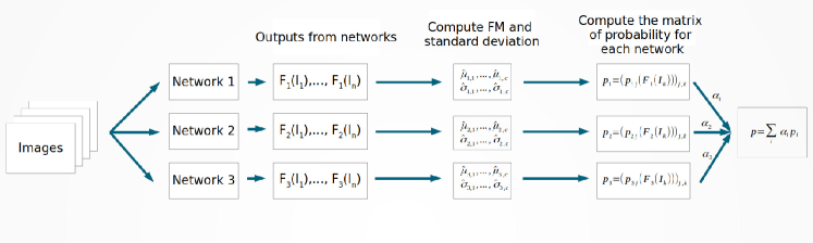
Figure 1: Illustration of our ensemble method.

3 Experiments

In this section, we present experiments for both the parametric and the non-parametric model on four publicly available datasets: CIFAR-10, CIFAR-100, MNIST, EMNIST-letters (with English alphabet only) [8], EMNIST. A brief description for each of the datasets is given below.

• The CIFAR-10 dataset consists of 60,000 $32\times 32$ color images from 10 classes, of which 50,000 are used for training and the rest are used for testing.

• The CIFAR-100 dataset consists of 60,000 $32\times 32$ color images from 100 classes, of which 50,000 are used for training and the rest are used as test data.

• The MNIST dataset consists of 70,000 $28\times 28$ grey images of handwritten digits 0 9, of which 60,000 are used for training and the rest are used as test data.

• The EMNIST-letters dataset consists of 145,600 $28\times 28$ grey images of handwritten English alphabets (26 classes), of which 124,800 are used for training and the rest for testing.

• The EMNIST-balanced dataset consists of 131,600 $28\times 28$ grey images of handwritten alphabets and digits in 47 classes (merging those alphabets with similar uppercase and lowercase, e.g. C, O), of which 112,800 are used for training and the rest for testing.

An outline of the entire procedure used in the experiments is presented below:

1. Train 20 CNNs $N_{1},...,N_{20}$ for each dataset. The choice of CNN can be arbitrary and in order to show the power of our proposed ensemble technique, we trained the networks for only a few epochs to yield “weak” networks. Here, for the sake of convenience, we choose the following architectures (all the models we used in this experiment are based on the models provided by keras [6] and modified slightly to meet our needs):

   1. CIFAR-10 We chose ResNet[15] with 20 weight layers and train these networks for only 3 epochs. The classification accuracies of these networks range from 61.6% to 72.8% and the average accuracy is 67.02%.

   2. CIFAR-100 We chose ResNet with 56 weight layers and train these networks for 50 epochs. The classification accuracies of these networks range from 59.1% to 63.5% and the average accuracy is 61.71%.

   3. MNIST We chose a very simple CNN with only one convolution layer and one fully-connected layer and train these networks for only 1 epoch. The classification accuracies of these networks range from 89.8% to 93.2% and the average accuracy is 90.89%.

   4. EMNIST-letters We chose a CNN with 2 convolution layer and 2 fully-connected layer and train these networks for only 1 epoch. The classification accuracies of these networks range from 89.8% to 93.2% and the average accuracy is 90.24%.

   5. EMNIST-balanced We chose a CNN with 2 convolution layer and 2 fully-connected layer and train these networks for only 1 epoch. The classification accuracies of these networks range from 82.1% to 83.7% and the average accuracy is 82.94%.

2. Compute the estimated weights $\alpha_{i}$, $i=1,...,20$ using Algorithm 1.

3. Combine these networks and compute the classification accuracy on the test data.

The results are shown in Table 1.

	Ave. Acc.	Param.	Non-param.
CIFAR-10	67.02%	75.99%	79.5%
CIFAR-100	61.71%	65.71%	73.14%
MNIST	90.89%	93.55%	93.58%
EMNIST-letters	90.24%	91.52%	91.61%
EMNIST-balanced	82.94%	84.27%	85.66 %

Table 1: Accuracies of the four datasets for parametric and non-parametric model

The result shows clearly that the proposed method works quite well and as we expected, when the networks are strong there is not much leeway to improve. On the contrary, when the networks are weak, the improvement is very significant. We can also see that the difference between parametric and non-parametric models decreases as the networks get stronger. Since obviously the features from those being classified correctly and those being classified incorrectly are not from the same distribution, in such cases, using a single Gaussian is not appropriate. When the networks are stronger, the difference between a single Gaussian distribution and the kernel density estimate is smaller. The motivation to use the parametric model when it performs almost as good as non-parametric model is clear: the non-parametric model takes 2 to 5 times longer than the parametric model.

In practice, we would like to know whether this ensemble technique reduces the time needed to achieve a certain accuracy. To answer this question, we run a experiment based on CIFAR-10 and the parametric ensemble model. The experiment goes as follow:

1. We trained 5 networks on CIFAR-10 using the same architecture as in the previous experiment.

2. Ensemble the intermediate models after running different number of epochs.

The result is shown in Figure 2. As we can see, the ensemble network performed constantly better. Since our ensemble method requires multiple networks, when comparing the efficiency of our method and the traditional CNN, it is better to consider the effective number of epochs, e.g., if we combine 5 networks and each of them is trained for 10 epochs, then the effective number of epochs would be $5\times 10=50$. Table 2 shows the result of this experiment in terms of the effective number of epochs. The table is to be interpreted as follows: on CIFAR-10, training a network with 50 epochs gives a classification accuracy 76.66% while training 5 networks, each with 10 epochs, and building the ensemble classifier based on these five networks gives a classification accuracy 80.06%. The message is that if you train multiple networks and build the ensemble network, you will get a better performance.

Another advantage of our ensemble method is that we can run multiple networks on different machines in parallel and then combine them without any retraining. The extra optimization step for finding the weights $\left\{\alpha_{i}\right\}$ takes less than a few minutes in all our experiments.

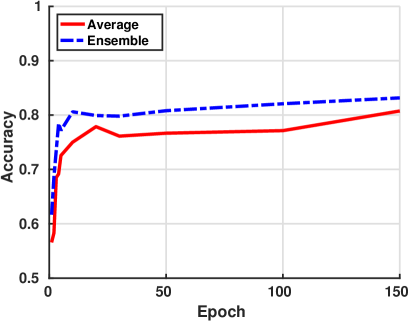
Figure 2: The comparison between the average accuracy of 5 networks and the accuracy of the ensemble networks: the dashed line is the ensemble network and the solid line is the average accuracy of the 5 networks.

Epochs	20($5\times 4$)	50($5\times 10$)	100($5\times 20$)
Ave.	77.86%	76.66%	77.13%
Ensemble	78.46%	80.6%	79.91%

Table 2: Average accuracy of networks and the accuracy of our parametric ensemble network at different effective number of epochs. The ensemble configuration is indicated in the parentheses: number of networks $\times$ number of epochs per network.

The third experiment is based ensemble classifiers using the intermediate features instead of the final outputs. The experiment is performed on MNIST, using weak classifiers based on two HOG features [9] (with two different configuration) and the Daisy feature [41]. Each weak classifier is built using the mixture model described in Section 2, i.e., the special case when there is only one network. The average accuracy of these three weak classifiers is 85.16% and the accuracy of the ensemble classifier is 88.6%. The result again shows capability of our ensemble method to boost the performance without re-training.

4 Conclusions

In this paper we presented a novel aggregation technique to combine “weak” networks/algorithms in order to boost the classification accuracy over each constituent of the aggregate. Traditional boosting requires re-training of every constituent of the aggregate and in contrast, our aggregation model does not require any re-training. This makes our aggregation model quite attractive from a computational cost perspective. We presented both parametric and non-parametric aggregation techniques and demonstrated via experiments the efficiency of the proposed methods. Another key advantage of our technique stems from the fact that it can cope with aggregation of features of distinct dimensions that are likely to result from using either different networks or even hand-crafted features that are extracted from the data. These salient features make our aggregation model unique. We presented several experiments demonstrating the performance of our proposed aggregation technique on widely used image databases in computer vision literature.

Acknowledgements: This research was funded in part by the NSF grant IIS-1525431 and IIS-1724174 to BCV.

References

- [1] Bijan Afsari. Riemannian lp center of mass: existence, uniqueness, and convexity. Proceedings of the American Mathematical Society, 139(2):655–673, 2011.
- [2] Forest Agostinelli, Michael R Anderson, and Honglak Lee. Adaptive multi-column deep neural networks with application to robust image denoising. In Advances in Neural Information Processing Systems, pages 1493–1501, 2013.
- [3] Shun-ichi Amari. Information geometry and its applications. Springer, 2016.
- [4] Rudrasis Chakraborty and Baba Vemuri. Statistics on the (compact) stiefel manifold: Theory and applications. arXiv preprint arXiv:1708.00045, 2017.
- [5] François Chollet. Xception: Deep learning with depthwise separable convolutions. arXiv preprint, 2016.
- [6] François Chollet et al. Keras, 2015.
- [7] Dan Ciregan, Ueli Meier, and Jürgen Schmidhuber. Multi-column deep neural networks for image classification. In Computer vision and pattern recognition (CVPR), 2012 IEEE conference on, pages 3642–3649. IEEE, 2012.
- [8] Gregory Cohen, Saeed Afshar, Jonathan Tapson, and André van Schaik. Emnist: an extension of mnist to handwritten letters. arXiv preprint arXiv:1702.05373, 2017.
- [9] Navneet Dalal and Bill Triggs. Histograms of oriented gradients for human detection. In Computer Vision and Pattern Recognition, 2005. CVPR 2005. IEEE Computer Society Conference on, volume 1, pages 886–893. IEEE, 2005.
- [10] Jia Deng, Wei Dong, Richard Socher, Li-Jia Li, Kai Li, and Li Fei-Fei. Imagenet: A large-scale hierarchical image database. In Computer Vision and Pattern Recognition, 2009. CVPR 2009. IEEE Conference on, pages 248–255. IEEE, 2009.
- [11] Li Deng. The mnist database of handwritten digit images for machine learning research [best of the web]. IEEE Signal Processing Magazine, 29(6):141–142, 2012.
- [12] Thomas G Dietterich. Ensemble methods in machine learning. In International workshop on multiple classifier systems, pages 1–15. Springer, 2000.
- [13] Maurice Fréchet. Les éléments aléatoires de nature quelconque dans un espace distancié. In Annales de l’institut Henri Poincaré, volume 10, pages 215–310. Presses universitaires de France, 1948.
- [14] Ross Girshick, Jeff Donahue, Trevor Darrell, and Jitendra Malik. Rich feature hierarchies for accurate object detection and semantic segmentation. In Proceedings of the IEEE conference on computer vision and pattern recognition, pages 580–587, 2014.
- [15] Kaiming He, Xiangyu Zhang, Shaoqing Ren, and Jian Sun. Deep residual learning for image recognition. In Proceedings of the IEEE conference on computer vision and pattern recognition, pages 770–778, 2016.
- [16] Geoffrey Hinton, Oriol Vinyals, and Jeff Dean. Distilling the knowledge in a neural network. arXiv preprint arXiv:1503.02531, 2015.
- [17] Forrest Iandola, Matt Moskewicz, Sergey Karayev, Ross Girshick, Trevor Darrell, and Kurt Keutzer. Densenet: Implementing efficient convnet descriptor pyramids. arXiv preprint arXiv:1404.1869, 2014.
- [18] Alex Krizhevsky, Vinod Nair, and Geoffrey Hinton. The cifar-10 dataset. online: http://www. cs. toronto. edu/kriz/cifar. html, 2014.
- [19] Alex Krizhevsky, Ilya Sutskever, and Geoffrey E Hinton. Imagenet classification with deep convolutional neural networks. In Advances in neural information processing systems, pages 1097–1105, 2012.
- [20] Yann LeCun. The mnist database of handwritten digits. nec research institute, 1998.
- [21] Yann LeCun, Yoshua Bengio, et al. Convolutional networks for images, speech, and time series. The handbook of brain theory and neural networks, 3361(10):1995, 1995.
- [22] Yann LeCun, Yoshua Bengio, and Geoffrey Hinton. Deep learning. nature, 521(7553):436, 2015.
- [23] David G Lowe. Object recognition from local scale-invariant features. In Computer vision, 1999. The proceedings of the seventh IEEE international conference on, volume 2, pages 1150–1157. Ieee, 1999.
- [24] Berger Marcel. A Panoramic View of Riemannian Geometry. Springer, 2003.
- [25] Mohammad Moghimi, Serge J Belongie, Mohammad J Saberian, Jian Yang, Nuno Vasconcelos, and Li-Jia Li. Boosted convolutional neural networks. In BMVC, 2016.
- [26] Sinno Jialin Pan and Qiang Yang. A survey on transfer learning. IEEE Transactions on knowledge and data engineering, 22(10):1345–1359, 2010.
- [27] Omkar M Parkhi, Andrea Vedaldi, Andrew Zisserman, et al. Deep face recognition. In BMVC, volume 1, page 6, 2015.
- [28] Shaoqing Ren, Kaiming He, Ross Girshick, and Jian Sun. Faster r-cnn: Towards real-time object detection with region proposal networks. In Advances in neural information processing systems, pages 91–99, 2015.
- [29] Mohammad J Saberian and Nuno Vasconcelos. Multiclass boosting: Theory and algorithms. In Advances in Neural Information Processing Systems, pages 2124–2132, 2011.
- [30] Hesamoddin Salehian, Rudrasis Chakraborty, Edward Ofori, David Vaillancourt, and Baba C Vemuri. An efficient recursive estimator of the fréchet mean on a hypersphere with applications to medical image analysis. Mathematical Foundations of Computational Anatomy, 2015.
- [31] Robert E Schapire. The boosting approach to machine learning: An overview. In Nonlinear estimation and classification, pages 149–171. Springer, 2003.
- [32] Holger Schwenk. The diabolo classifier. Neural Computation, 10(8):2175–2200, 1998.
- [33] Holger Schwenk and Yoshua Bengio. Adaboosting neural networks: Application to on-line character recognition. In International Conference on Artificial Neural Networks, pages 967–972. Springer, 1997.
- [34] Holger Schwenk and Yoshua Bengio. Boosting neural networks. Neural computation, 12(8):1869–1887, 2000.
- [35] Pierre Sermanet, David Eigen, Xiang Zhang, Michaël Mathieu, Rob Fergus, and Yann LeCun. Overfeat: Integrated recognition, localization and detection using convolutional networks. arXiv preprint arXiv:1312.6229, 2013.
- [36] Karen Simonyan and Andrew Zisserman. Very deep convolutional networks for large-scale image recognition. arXiv preprint arXiv:1409.1556, 2014.
- [37] Yi Sun, Yuheng Chen, Xiaogang Wang, and Xiaoou Tang. Deep learning face representation by joint identification-verification. In Advances in neural information processing systems, pages 1988–1996, 2014.
- [38] Yi Sun, Xiaogang Wang, and Xiaoou Tang. Deep learning face representation from predicting 10,000 classes. In Proceedings of the IEEE Conference on Computer Vision and Pattern Recognition, pages 1891–1898, 2014.
- [39] Christian Szegedy, Sergey Ioffe, Vincent Vanhoucke, and Alexander A Alemi. Inception-v4, inception-resnet and the impact of residual connections on learning. In AAAI, pages 4278–4284, 2017.
- [40] Christian Szegedy, Wei Liu, Yangqing Jia, Pierre Sermanet, Scott Reed, Dragomir Anguelov, Dumitru Erhan, Vincent Vanhoucke, and Andrew Rabinovich. Going deeper with convolutions. In Proceedings of the IEEE conference on computer vision and pattern recognition, pages 1–9, 2015.
- [41] Engin Tola, Vincent Lepetit, and Pascal Fua. Daisy: An efficient dense descriptor applied to wide-baseline stereo. IEEE transactions on pattern analysis and machine intelligence, 32(5):815–830, 2010.
- [42] Matthew D Zeiler and Rob Fergus. Visualizing and understanding convolutional networks. In European conference on computer vision, pages 818–833. Springer, 2014.