Measurements and Modeling of Near-Surface Radio Propagation in
Glacial Ice and Implications for Neutrino Experiments

Abstract

We present measurements of radio transmission in the $\sim 100$ MHz range through a $\sim 100$ m deep region below the surface of the ice at Summit Station, Greenland, called the firn. In the firn, the index of refraction changes due to the transition from snow at the surface to glacial ice below, affecting the propagation of radio signals in that region. We compare our observations to a finite-difference time-domain (FDTD) electromagnetic wave simulation, which supports the existence of three classes of propagation: a bulk propagation ray-bending mode that leads to so-called “shadowed” regions for certain geometries of transmission, a surface-wave mode induced by the ice/air interface, and an arbitrary-depth horizontal propagation mode that requires perturbations from a smooth density gradient. In the non-shadowed region, our measurements are consistent with the bulk propagation ray-bending mode both in timing and in amplitude. We also observe signals in the shadowed region, in conflict with a bulk-propagation-only ray-bending model, but consistent with FDTD simulations using a variety of firn models for Summit Station. The amplitude and timing of our measurements in all geometries are consistent with the predictions from FDTD simulations. In the shadowed region, the amplitude of the observed signals is consistent with a best-fit coupling fraction value of $2.4$% (0.06% in power) or less to a surface or horizontal propagation mode from the bulk propagation mode. The relative amplitude of observable signals in the two regions is important for experiments that aim to detect radio emission from astrophysical high-energy neutrinos interacting in glacial ice, which rely on a radio propagation model to inform simulations and perform event reconstruction.

I Introduction

Experiments that aim to detect impulsive radio emission in the $\sim 100$ MHz – 1 GHz range created by high-energy astrophysical or cosmogenic neutrinos interacting in glacial ice require an understanding of radio propagation through glacial ice. In the bulk ice, this is presumed to be straightforward – rays propagate along straight lines in the glacial ice where the ice density and index of refraction are nearly constant. However, in the $\sim 100$ m or more below the upper surface of the ice, the snow at the surface slowly transitions from loose snow to glacial ice below in a region called the firn. This firn region represents a density gradient from that of loose snow to that of ice Arthern et al. (2013); Koci and Kuivinen (1983), corresponding to an index of refraction of $n\approx 1.35$ for the snow near the surface to $n=1.78$ for bulk ice in the radio frequency range of interest for neutrino detection Avva et al. (2015); Barwick et al. (2018). Furthermore, annual variations in the firn mean that the gradient is not perfectly smooth – there are known layers in the firn, especially evident near the surface Hawley et al. (2008). The changing index of refraction causes the paths of electromagnetic waves to bend and scatter, affecting the propagation time and distance. To accurately calculate experimental sensitivity and reconstruct neutrino energy and arrival direction, the effects of propagation must be included in simulations and event reconstruction algorithms of in-ice neutrino experiments.

Ray-tracing models of radio propagation through the firn indicate that rays bend such that there is a so-called “shadow” region, where a receiver placed above a transmitter and horizontally displaced from that transmitter will not be able to see emission from the transmitter in certain geometries Barwick et al. (2018); ARA Collaboration et al. (2012); Vieregg et al. (2016). For neutrino detection, this means that neutrinos that interact in the shadow region of a given receiver cannot be seen by that receiver, and implies that a deeper receiver will be able to observe a larger instantaneous solid angle compared to a surface or near-surface receiver.

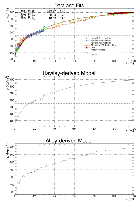
Figure 1: Top: Various firn density data sets recorded at or near Summit Station, using a variety of techniques Hawley et al. (2008); Alley and Koci (1988); Alley et al. (1997), and a model based on radio echo data at Summit Station Arthern et al. (2013). We fit a double exponential to all of the data shown, motivated by Herron and Langway (1980) and shown with the red line. From this, we choose to use two firn models for our analysis. Middle: The first model uses the Hawley neutron density probe data shallower than 30 m and the best-fit exponential deeper than 30 m Hawley et al. (2008). Bottom: The second model uses the Alley ice core data to 100 m, and the best-fit exponential at larger depths Alley and Koci (1988). The parameters of the best-fit double exponential are shown, where $\rho_{s}$ is the density at the surface in kg/m³, and $L_{1}$ and $L_{2}$ are the length scales in meters of each portion of the exponential fit.

Recently, observations of horizontally-propagating waves between transmitters deployed in the ice in shadowed regions relative to the receivers indicate that other propagation modes exist Barwick et al. (2018). Modes that include “surface,” “lateral,” and “leaky” waves are well-known solutions to Maxwell’s Equations at dielectric interfaces (see e.g. Frezza and Tedeschi (2015) for a pedagogical review). Previously, surface waves have been discussed as a possible mechanism for neutrino detection Ralston (2005), but previous measurements show no evidence for significant power in a surface-wave mode Besson et al. (2008); Alvarez et al. (2015). The recently-observed propagation consistent with a horizontally-propagating mode at arbitrary depth Barwick et al. (2018) has implications for determining the optimal geometry of neutrino detectors if the coupling to the horizontally-propagating modes is large. If the power contained in these modes is small compared to the ray-bending mode, then signals in this region would not contribute significantly to the effective volume of in-ice neutrino detectors.

We have made measurements of radio propagation through the firn at Summit Station, Greenland in June 2013 using a fast, impulsive, high-voltage transmitter placed a few feet below the surface and a receiver lowered down a borehole, up to 1050 ft. away and 600 ft. deep. At the largest depths, the receiver is well below the firn layer at Summit, which is measured to be $\sim~{}100$ m Arthern et al. (2013). We compare these measurements to models of electromagnetic wave propagation through the firn to constrain possible radio propagation modes.

In Section II, we discuss firn density models at Summit Station, a finite-difference time-domain (FDTD) simulation, and a ray-tracing algorithm that explores the bulk ray-bending propagation mode as well as surface-wave and arbitrary-depth horizontal propagation modes. In Section III, we present measurements of radio propagation through the firn at Summit Station in the $\sim 100$ MHz range. We then discuss the implications for radio detectors for high-energy neutrinos interacting in glacial ice in Section IV.

II Modeling of Radio Propagation in the Firn at Summit Station, Greenland

II.1 Firn Index of Refraction Model

To compare with measurements, we construct two different firn models, based on a variety of measurements of the density profile, $\rho(z)$, at and near Summit Station Hawley et al. (2008); Alley and Koci (1988); Alley et al. (1997); Arthern et al. (2013) to determine the index of refraction as a function of depth in meters ($z$) for the firn layer. The commonly-used Herron-Langway parameterization of firn models has two density regimes, each of which is fit by an exponential subtracted from an offset Herron and Langway (1980). The break point between the two exponential fits occurs at a depth corresponding to the critical density, $\rho_{c}$=550 kg/m³, above which the onset of jamming of snow grains leads to slower compactification Herron and Langway (1980). The data that we use to construct our models is shown in Figure 1. We perform a double exponential fit to all of the data, shown with the red line in Figure 1. The fit parameters are shown in Figure 1 as well, and using these parameters, we find a critical depth of 14.9 m and that $\rho(z)$ is given by:

$$\begin{split}\rho(z)=0.917-0.594e^{-z/30.8}\qquad z\leq 14.9\\ \rho(z)=0.917-0.367e^{-(z-14.9)/40.5}\qquad z>14.9.\end{split}$$ (1)

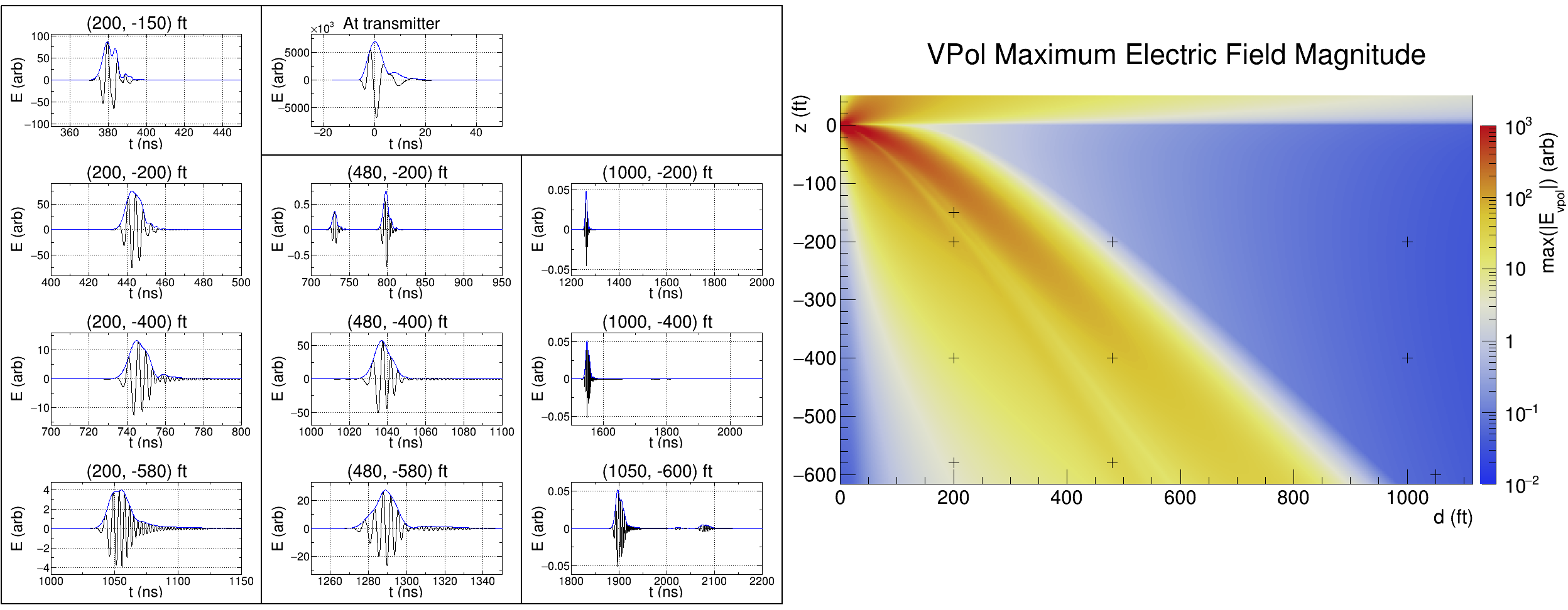
Figure 2: The result from the FDTD simulation using a best-fit of available data to a Herron-Langway firn model, described in Section II.1. Although the model is continuous, it is not differentiable at the critical density, producing an additional set of reflections. In the simulation, a dipole transmitter is placed 3 ft. below the surface of the snow, from which a band-limited impulse between 90-250 MHz propagates through the firn. The color map shows the maximum vertically-polarized electric field reached over the course of the simulation at each point. Each cross on the color map indicates a geometry where we placed a receiver at Summit Station relative to the transmitter location, which is set at (0, -3 ft.) here (see Section III.1 for further discussion). Resulting simulated waveforms (electric field as a function of time) are shown for the location of each cross and for the location of the transmitter. The relative amplitudes of the waveforms can be compared.

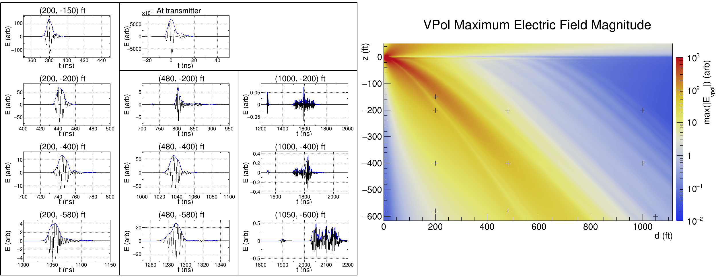
Figure 3: The result from the FDTD simulation using a firn model based on neutron scattering data from Hawley Hawley et al. (2008) and a global exponential fit to all data sets beyond 30 m, described in Section II.1. In the simulation, a dipole transmitter is placed 3 ft. below the surface of the snow, from which a band-limited impulse between 90-250 MHz propagates through the firn. The color map shows the maximum vertically-polarized electric field reached over the course of the simulation at each point. Each cross on the color map indicates a geometry where we placed a receiver at Summit Station. Resulting Each cross on the color map indicates a geometry where we placed a receiver at Summit Station relative to the transmitter location, which is set at (0, -3 ft.) here (see Section III.1 for further discussion). Resulting simulated waveforms (electric field as a function of time) are shown for the location of each cross and for the location of the transmitter. The relative amplitudes of the waveforms can be compared.

Horizontal propagation modes require perturbations from a smoothly-varying density gradient, motivating the use of models that include the real density fluctuations observed at Summit Station. We therefore construct two models that use different linearly-interpolated data sets over their entire range, and the best-fit exponential elsewhere. The first model consists of the neutron scattering data from Hawley Hawley et al. (2008) at depths smaller than 30 m and the best-global-fit exponential beyond 30 m. The second model uses measured densities from the Alley ice core data up to 100 m, since it is the only data set that spans such a large range of depths, and then the best-global-fit exponential beyond 100 m. By a depth of $\sim 100$ m, the firn has transitioned to glacial ice. These firn models are not perfect – the density profile changes each year due to snow accumulation and compaction and varies from site to site, the firn layers may be under sampled in the data, making both the neutron scattering and ice core data imperfect for our purposes.

For radio propagation in glacial ice, the dielectric constant ($\epsilon$) is related to the density (in g/cm³) of the ice Kovacs et al. (1995) by:

$$\epsilon^{\prime}=(1+0.845\rho)^{2},$$ (2)

allowing us to calculate the index of refraction $n=\sqrt{\epsilon^{\prime}}$ as a function of depth for the firn.

II.2 Finite-Difference Time-Domain (FDTD) Simulation

Previous studies of radio propagation in ice have used geometric optics, which is valid in regimes where the wavelength is much smaller than the feature sizes. Layers of ice near the surface contain features of sizes comparable to wavelengths (including the ice-air interface), so we have implemented the FDTD method Taflove and Hagness (2005), which numerically solves the wave equation on a time-space lattice. This powerful but computationally expensive time-domain treatment is particularly appropriate for propagation of the impulsive broadband emission expected to be generated by neutrinos. Our simulation software interfaces with the FDTD solver meep Oskooi et al. (2010) .

We use the cylindrical symmetry of a vertical dipole antenna to reduce the computation requirements. The transmitter is at horizontal distance $d=0$ and the ice surface is at $z=0$. $n(z)$ varies according to the chosen ice density model below the ice surface, and $n$=1 above the surface. We do not include attenuation or absorption in the ice in the simulation. Perfectly-matched layers (PMLs), which are absorptive across a range of frequencies, are placed at the edges of the computational domain to simulate propagation outside of the domain (otherwise waves would reflect off the edges of the computational domain).

We simulate a dipole transmitter at -3 ft. in a domain with $z\in[190,80]$ m and $d\in[0,360]$ m, with a 20 m PML located outside the volume. To keep the computational requirements modest, we use a grid resolution of 5 cm. At this resolution, numerical dispersion limits the maximum frequencies that may be reliably simulated to 300 MHz. We simulate a vertical dipole electric-field impulse with with a real component corresponding to the impulse response of a 90-250 MHz fourth-order digital Butterworth bandpass filter to roughly match the frequency content of our measurements, which are reported in Section III.

We perform simulations with the ice models described in Section II.1 above and record the maximum electric field magnitude achieved on a 0.5 m grid. We also record complete time domain information at the transmitter and at positions corresponding to our measurements. The results from the simulations are shown in Figures 2, 3, and 4. We note that beam pattern suppression from the dipole transmitter dominates at steep angles.

To investigate the effect of the depth of the transmitter and the frequency content of the signal, we vary these parameters in the simulation, and show the results in Figure 5. As the transmitter is lowered, the refractive ray-bending becomes less pronounced, and reflections off of the ice/air interface serve to further fill in the shadowed region. The simulations at all depths also show power beyond the predicted shadowed region (even after accounting for reflections off of the surface), which supports the idea that waves propagate along density perturbations in the firn. The amplitude of the signals seen in simulations in this region is significantly smaller than in the non-shadowed region at all depths.

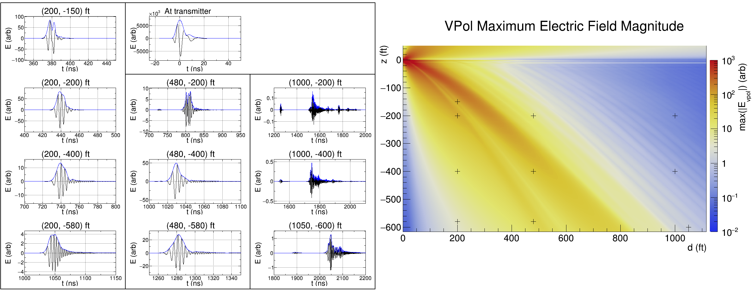
Figure 4: The result from the FDTD simulation using a firn model based on ice core data from Alley Alley and Koci (1988) and a global exponential fit to all data sets beyond 100 m, described in Section II.1. In the simulation, a dipole transmitter is placed 3 ft. below the surface of the snow, from which a band-limited impulse between 90-250 MHz propagates through the firn. The color map shows the maximum vertically-polarized electric field reached over the course of the simulation at each point. Each cross on the color map indicates a geometry where we placed a receiver at Summit Station relative to the transmitter location, which is set at (0, -3 ft.) here (see Section III.1 for further discussion). Resulting simulated waveforms (electric field as a function of time) are shown for the location of each cross and for the location of the transmitter. The relative amplitudes of the waveforms can be compared.

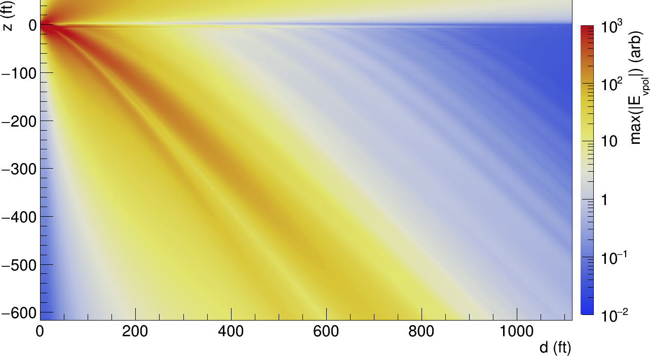
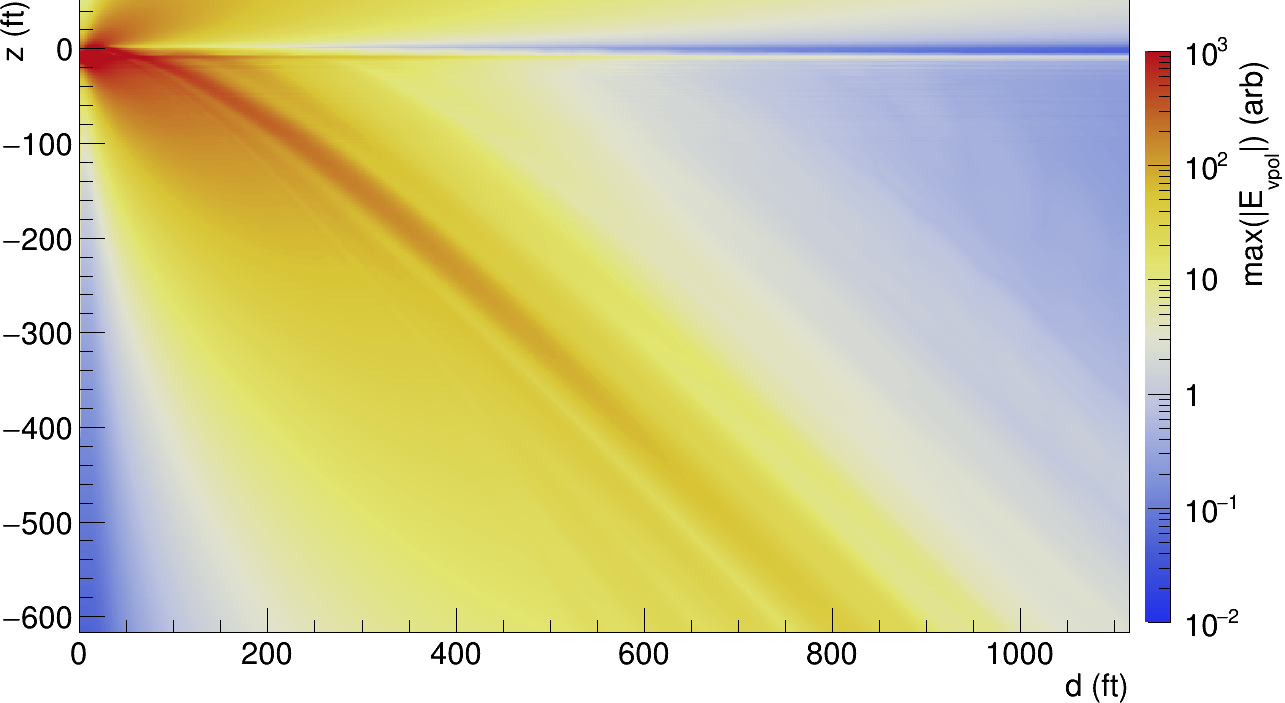
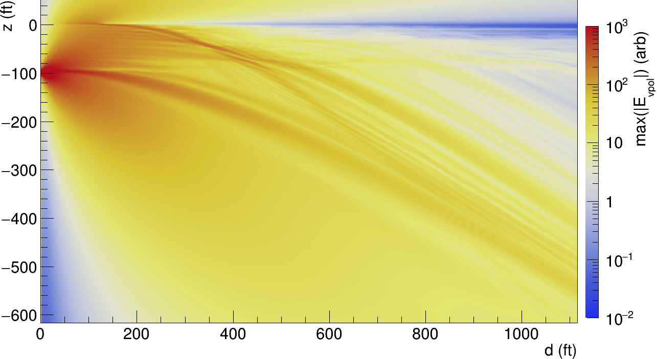
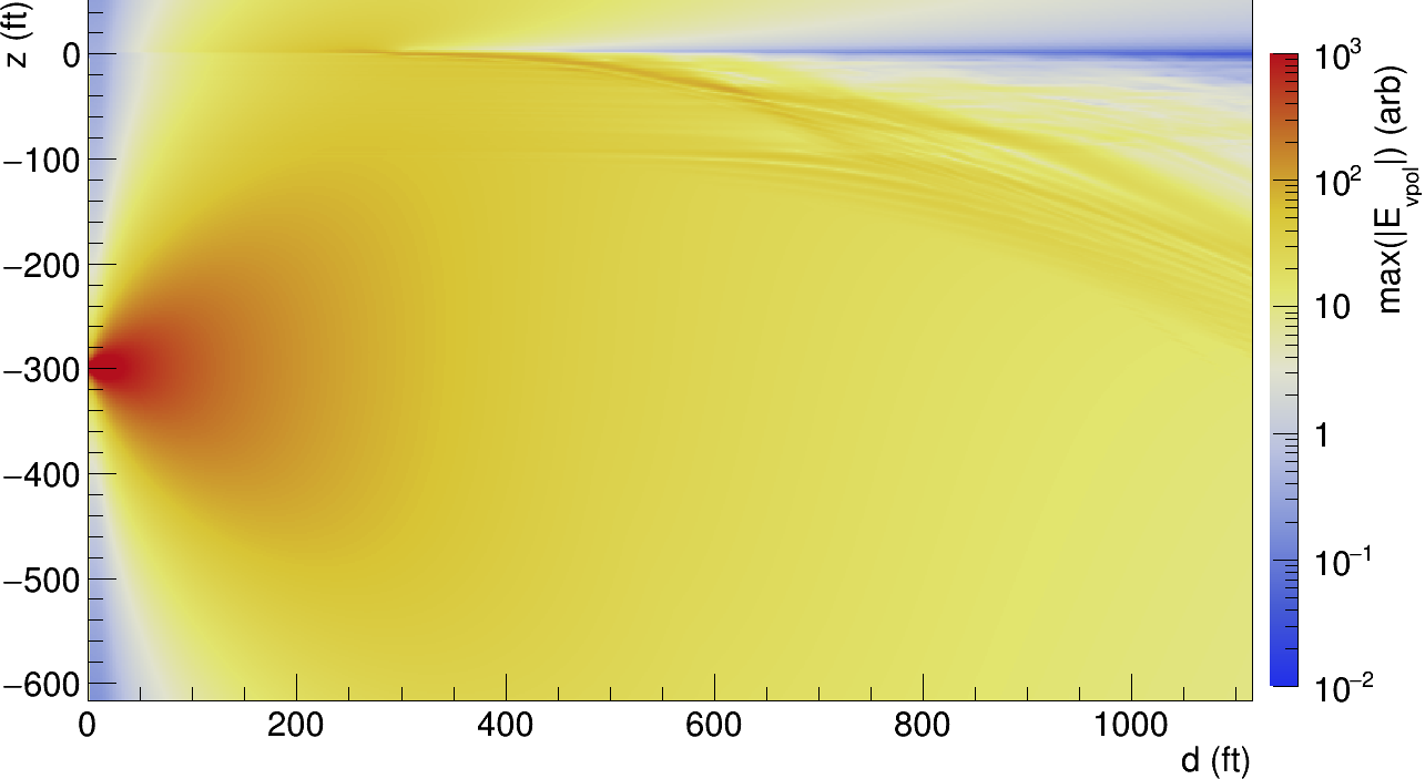
Figure 5: Variations on the FDTD simulation in Figure 3. Upper Left: The signal is 200-300 MHz instead of 90-250 MHz. Upper Right: The transmitter is placed 10 ft. below the surface instead of 3 ft. below. Lower Left: The transmitter is placed 100 ft. below the surface. Lower Right: The transmitter is placed 300 ft. below the surface. The firn model, based on neutron scattering data from Hawley Hawley et al. (2008) is kept the same. The color map shows the maximum vertically-polarized electric field magnitude reached over the course of the simulation at each point.

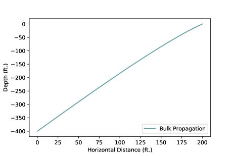
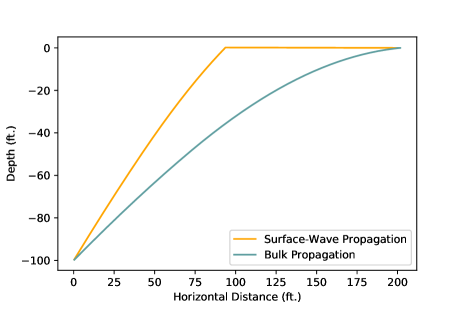
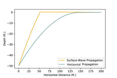
Figure 6: Example ray-tracing solutions given a transmitter and receiver depth. In each case shown here, the transmitter is just below the surface. Top: A geometry where only the bulk propagation (refractive ray-bending) mode yields a solution (Receiver Depth 400 ft., Transmitter Horizontal Distance 200 ft.). Middle: A geometry where the bulk propagation mode yields a solution and there is an additional surface-wave solution Ralston (2005) up to the TIR angle (Receiver Depth 100 ft., Transmitter Horizontal Distance 200 ft.). Bottom: A geometry where the bulk propagation mode yields no solution, but a horizontally-propagating solution Barwick et al. (2018) is found (Receiver Depth 50 ft., Transmitter Horizontal Distance 200 ft.). In these geometries, there is always also an additional surface-wave solution up to the TIR angle Ralston (2005).

The simulations indicate that although the signal is strongest in the non-shadowed zone, a signal is still present in all regions. For the non-smooth firn models, the region corresponding to the shadow of the transmitter contains two timescales of propagation. The earlier-arriving waves are present even with a smooth density profile, and are identified with “surface” or “lateral” waves. The second kind of propagation produces a longer train of signals and does not appear in a smooth density model, so it is likely from reflections between layers or channeling along peaks or troughs in the density profile. The details of the second signal depend strongly on the firn model, transmitter depth, and frequency content of the signal. Qualitatively, the relative amplitude of the first and second signal changes as a function of depth, with the first signal growing stronger with respect to the second at larger depths.

On top of the effect of the beam pattern of the simulated transmitter, the simulation predicts additional significant spatial variations in maximum electric field having to do with interference between different paths, even in the non-shadowed region, visible in the colormaps in Figures 3 and 4. The presence of these amplitude variations makes amplitude predictions dependent on the ice model and frequency content of the signal.

II.3 Ray Tracing

We perform additional ray-tracing studies to investigate if it is possible to model in a simple way the three different modes suggested by the FDTD simulations in Section II.2. We place a transmitter near the surface and a receiver at a chosen depth, $z$, and horizontal distance, $d$, from the transmitter, and find the ray that connects the transmitter and receiver location for each of three modes. The first mode is the bulk refractive propagation mode, corresponding to standard geometric optics, which predicts ray-bending in the firn and therefore a shadowed region. The second is a surface-wave propagation mode, discussed in Ralston (2005), where for rays that hit the ice/air interface at the total internal reflection (TIR) angle ($48^{\circ}$) or steeper, a fraction of the power will couple to a surface wave. Here we model this as propagating along the surface and losing electric field strength as $1/\sqrt{r}$ due to being confined to two dimensions. The third is an arbitrary-depth horizontal propagation mode, where for rays that become horizontal due to refractive ray-bending, a fraction of the power couples to a horizontal mode if there is a specific class of perturbation from a smooth density gradient at that depth, as may occur in firn layers due to annual snow deposits Barwick et al. (2018). We allow for two-dimensional ($1/\sqrt{r}$) or three-dimensional ($1/r$) propagation. We call these modes “bulk”, “surface”, and “horizontal” propagation, respectively.

For a transmitter placed just below the surface, one or two of the three ray-tracing propagation modes will find a valid solution for an arbitrarily-chosen $z$ and $d$, as shown in Figure 6. In the non-shadowed region (top and middle panels), there can also be a set of surface-wave solutions (middle panel). In the shadowed region (bottom panel), there is always both a horizontal and surface-wave solution for a transmitter placed near the surface.

III Firn Propagation Measurements at Summit Station, Greenland

III.1 Experimental Setup

A schematic of our experimental design is shown in Figure 7. We used a 6 kV FID Technologies pulser triggered by an external TTL signal to generate impulsive radio signals with power in the 100 MHz – 1 GHz range. We transmitted the signal from a low-gain fat dipole antenna, built for the RICE experiment Kravchenko et al. (2003) at the South Pole. An identical receiving antenna was placed a distance away, and the received signal was first sent through an attenuator (as needed, depending on the physical configuration of the transmitter and receiver), followed by a Miteq AFS3-00200120-10-1P-4-L amplifier with 50 dB of gain. We read the signals out using a Tektronix MSO5204B oscilloscope, which was triggered on a different channel using the same signal generator that triggered the high voltage FID Technologies pulser. The oscilloscope recorded waveforms with 10,000 averages so that the noise level in recorded waveforms is small. We used Times Microwave LMR-600, LMR-240, and LMR-200, and cable lengths are given in Figure 7.

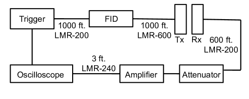
Figure 7: A schematic of the electronics layout for our experimental setup. A 6 kV FID Technologies pulser triggered by an external TTL signal was used to send signals to the transmitting low-gain antenna. After the signal was received by the receiving antenna, it was attenuated (in some geometries) and then amplified using a low-noise Miteq amplifier and read out using an oscilloscope, which was triggered using the same TTL signal that triggered the FID Technologies pulser.

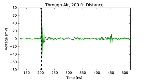
Figure 8: The received signal, using the experimental setup shown in Figure 7, with the transmitting and receiving antennas separated by 200 ft. in the air. For this measurement, the antennas were placed $\sim 4$ ft. above the surface of the snow on empty wooden crates. The time shown is the absolute propagation time of the signal after removing the system delay. The dashed line shows the predicted time of flight. The second pulse seen at 245 ns after the initial pulse is a known reflection in the system corresponding the out-and-back time along one section of LMR-600 cable, and appears in all data. Because we did not record the overall attenuation setting for this measurement, the amplitude information is not comparable to the downhole measurements.

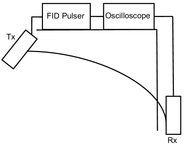
Figure 9: A simplified schematic of the experimental setup, as deployed at Summit Station, Greenland. The receiving antenna was placed down a borehole that was filled with drilling fluid to $\sim 100$ ft. depth, and the feed of the transmitting antenna was placed $\sim~{}3$ ft. below the surface using an auger drill. The front-end electronics and triggering scheme are the same as in the in-air measurements shown in Figure 7.

To determine the absolute delay of our system, we first made a measurement with the transmitter and receiver separated by 200 ft. horizontally in the air. The antennas were placed on top of wooden crates, $\sim 4$ ft. above the surface of the snow. The received in-air waveform is shown in Figure 8. The in-air signals show a system delay of 2395 ns, which we then subtract from each subsequent measurement of time of flight with the receivers placed in the ice. We did not record the overall attenuation setting for the in-air measurement relative to the downhole measurements discussed below, so the amplitude of the in-air pulse is not comparable to the downhole measurements. The in-air pulse measured with our system has a pass band from 190–270 MHz, measured at its -3 dB points and defined by the antenna and amplifier response and the loss in the cables as a function of frequency. When the antennas are embedded in the ice, we expect the frequency response of the antennas to go down.

There is a reflection in our system, obvious in the data in Figure 8, that arrives 245 ns after the initial pulse. The relative timing of the reflection did not change as we changed the distance between the antennas or moved the antennas closer or farther from the surface. We surmise that this is from a reflection in the system, as it is present in all data and corresponds to the out-and-back propagation delay from 100 ft. of LMR-600 cable, segments of which are present in the system. Other than this reflection in the system, the in-air measurements show a clean impulse.

We took data using our system with a variety of transmitter and receiver geometries. The layout is shown in Figure 9. We lowered the receiver down the DISC borehole at Summit Station, which has a plastic casing along the upper $\sim 100$ ft. and is filled with non-conductive drilling fluid below $\sim 100$ ft. We used an auger drill to make shallow holes at the surface to place the transmitting antenna into, so that the antenna feed was $\sim 3$ ft. below the surface of the snow to ensure good coupling to the snow. At each transmitter location, we drilled these shallow holes at a variety of angles with respect to the vertical and looked for the angle at which the signal strength was strongest to ensure that the antenna was broadside to the path of propagation. We could not perform a similar procedure for the receiver down the borehole, so we calculate a correction to the amplitude due to the beam pattern of the dipole antenna down the hole based on the incidence angles predicted by our ray tracer and a $\sin\theta$ antenna beam pattern in electric field to use as an uncertainty in the calculations in Section III.4.

When the receiving antenna passed below the level of the drilling fluid in the borehole, we saw an increase in signal strength, which indicates improved coupling to the ice. This effect was repeatable and clearly related to entering and exiting the fluid. We therefore only report on measurements at depths below 100 ft., since there is a discontinuity in amplitudes at a depth of 100 ft.

Rx	Horiz. Tx	Meas. ToF,	Meas. ToF,	Ray-trace ToF	Ray-trace ToF	Ray-trace ToF	FDTD ToF	FDTD ToF
Depth	Dist.	1st Pulse	2nd Pulse	(Bulk Prop.)	(Horiz. Prop.)	(Surf. Prop.)	1st Pulse	2nd Pulse
(ft.)	(ft.)	(ns)	(ns)	(ns)	(ns)	(ns)	(ns)	(ns)
Non-Shadowed Region in All Firn Models
150	200	388	–	$377\pm 1$	–	$391\pm 7$	$379\pm 1$	–
200	200	441	–	$438\pm 2$	–	$446\pm 2$	$440\pm 1$	–
400	200	755	–	$737\pm 3$	–	–	$742\pm 4$	–
580	200	1072	–	$1038\pm 3$	–	–	$1053\pm 4$	–
400	480	1035	–	$1025\pm 3$	–	$1054\pm 13$	$1033\pm 5$	–
580	480	1295	–	$1272\pm 4$	–	$1287\pm 3$	$1285\pm 5$	–
Edge of the Shadowed Region
200	480	806	–	$782\pm 7$	$782\pm 7$	$809\pm 27$	$808\pm 7$	–
Shadowed Region in All Firn Models
200	1000	1315	1560	–	$1442\pm 33$	$1484\pm 74$	$1259\pm 1$	$1562\pm 36$
400	1000	1601	1790	–	$1682\pm 20$	$1729\pm 60$	$1545\pm 4$	$1786\pm 54$
600	1050	1873	2010	–	$1998\pm 12$	$2052\pm 53$	$1893\pm 4$	$2051\pm 35$

Table 1: The measured and expected time of flight for a variety of experimental configurations, ray-tracing hypotheses, and FDTD simulations. For the ray-tracing hypotheses and FDTD simulations, we use two different firn models, which are based on the Hawley Hawley et al. (2008) and Alley Alley and Koci (1988) data, and are discussed in Section II.1. We report the mean of the results for each firn model and the standard deviation as an uncertainty. The time of flight shown for the data and the FDTD simulations is the arrival of the maximum amplitude of the signal. For the 600 ft. depth and 1050 ft. distance measurement, we report an uncertainty on the second pulse’s arrival time that accounts for the observation of multiple peaks of comparable amplitude. In both the shadowed and the non-shadowed region, the data is more consistent with the results of the FDTD simulations than the ray tracer. In the non-shadowed region, the data matches the predicted time of flight well, with $\sim 1$% agreement with the FDTD simulations and $\sim 3$% agreement to the bulk propagation ray-tracing mode. We observe signals in the shadowed region, and the timing of the first pulse is consistent with FDTD simulations to within 3% and differs from the ray tracer prediction for horizontal propagation by 9%.

Rx	Horiz. Tx	Measured	Relative	Relative E-field	Tx Angle
Depth (ft.)	Distance (ft.)	Voltage (mV)	Voltage (Arbitrary)	FDTD Simulation (Arbitrary)	(Degrees)
Non-Shadowed Region in All Firn Models
150	200	776	1.00	$1.00\pm 0.30$	17
200	200	627	0.81	$0.71\pm 0.09$	28
400	200	431	0.56	$0.12\pm 0.01$	54
580	200	137	0.18	$0.04\pm 0.001$	64
400	480	182	0.23	$0.63\pm 0.23$	8
580	480	236	0.30	$0.13\pm 0.15$	30
Edge of the Shadowed Region
200	480	59	0.076	$0.07\pm 0.01$	0
Shadowed Region in All Firn Models
200	1000	1.3	$1.7\times 10^{-3}$	$4.8\times 10^{-4}\pm 1\times 10^{-5}$	0
400	1000	1.5	$1.9\times 10^{-3}$	$5.0\times 10^{-4}\pm 1\times 10^{-5}$	0
600	1050	2.1	$2.7\times 10^{-3}$	$5.0\times 10^{-4}\pm 1\times 10^{-5}$	0

Table 2: The measured signal peak-to-peak amplitudes of the first received signal for a variety of experimental configurations (receiver depth and transmitter horizontal distance), after accounting for relative attenuation in the system between different configurations. Signals in the shadowed region are uniformly smaller than signals in the non-shadowed region, even after accounting for signal path length differences. The fourth column shows the measured voltages, normalized to the first row, for direct comparison to the values in the fifth column. The fifth column shows the amplitude of the first signal predicted by the FDTD simulations assuming firn models based on the Hawley data Hawley et al. (2008) and the Alley ice core data Alley and Koci (1988) (discussed in Section II.1). We report the mean of the simulation results using the two firn models and the standard deviation as an uncertainty. The simulation assumes a dipole transmitter and an isotropic receiver and does not include any electric field loss from attenuation in the ice. The amplitudes predicted from the FDTD simulation show significant suppression at steep angles due to the beam pattern of the simulated transmitter (most prominent at the 580 ft. depth, 200 ft. horizontal distance geometry), which would not appear in the data, since we optimized the transmitter angle for the measurements. The predicted elevation angle (with respect to horizontal) of the transmission from the ray tracer is shown in the last column.

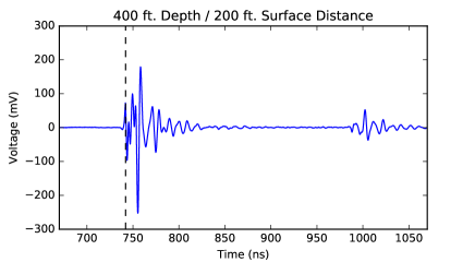
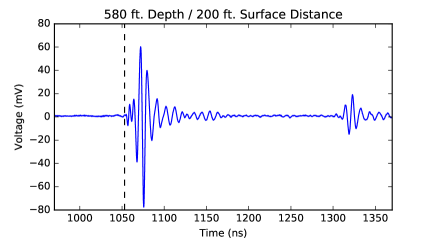
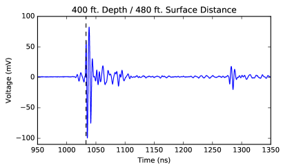
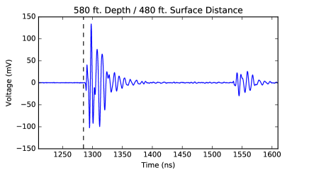
Figure 10: Top two: Example waveforms from locations where there is only a bulk propagation ray-bending solution. Bottom two: Example waveforms from locations where there is a bulk propagation ray-bending solution and an additional surface-wave solution. The time shown is the absolute propagation time of the signal after removing the system delay. The dashed line shows the predicted time of flight from the FDTD simulations, shown in Table 1. The second pulse seen at 245 ns after the initial pulse is a known reflection in the system corresponding the out-and-back time along one section of LMR-600 cable, and appears in all data. There is no evidence that a large fraction of power is contained in an additional horizontally-propagating surface wave for the waveforms shown in the bottom panels, which would arrive up to 20 ns after the first signal (times shown in Table 1).

Table 1 shows the measured time of flight of the signals observed compared to the expected time of flight from the three modes described in Section II.3 and the simulated time of flight from the FDTD simulations described in Section II.2. We estimate that we measure the transmitter distance across the surface to within 3 ft. and the receiver depth down the borehole to within 1 ft., using a measuring tape. We include the time of flight for the first observed pulse, and for cases where we saw a second pulse (separate from the known reflection in the system), we report its time of flight as well. Note that for each geometry, only one or two modes out of the three in the ray tracer converge on a solution. In the non-shadowed region, the time of flight matches the FDTD simulation results within 1%. In the shadowed region, the time of flight is uniformly less consistent with the predictions. The uncertainty on the predicted time of flights from using different firn models is larger for the second pulse. This is consistent with the first pulse’s surface wave origin, and the second pulse originating from horizontal propagation along layers in the firn, which change from model to model. The measured arrival times match the FDTD simulation results in the shadowed region to within 3%.

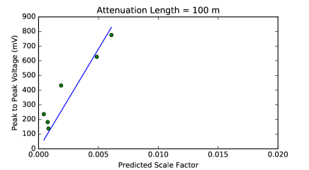
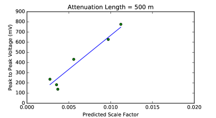
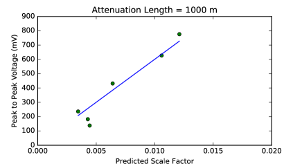
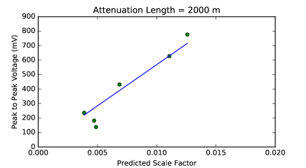
Figure 11: Green points: The peak-to-peak voltage measured for the largest (and first to arrive in all cases) signal in the non-shadowed region vs. a predicted scale factor compared to a receiver at 1 m for a given field attenuation length and assuming $1/r$ scaling for electric field. Blue line: A least squares linear fit to the data, given the assumed attenuation length and $1/r$ scaling in each case. The slope of this line is used to derive the presumed electric field at 1 m from the transmitter in each case and errors corresponding to the full spread of values are derived from fitting a line to only one measurement at a time. The results are shown in Table 3.

Table 2 shows the measured amplitude (peak-to-peak voltage) of the signals seen for each geometry and the predicted amplitudes from the FDTD simulation. The FDTD simulation assumes a dipole transmitter and an isotropic receiver and does not include any electric field loss from attenuation in the ice. At the largest distance reported, the path length is smaller than one $e$-folding, assuming previously-reported attenuation lengths at Summit Station Avva et al. (2015); MagGregor et al. (2015). The signals at the 1000 ft. and 1050 ft. horizontal transmission distance were so weak that we removed a 20 dB attenuator from the system in order to see the signals. This has already been accounted for in the numbers reported in this table. Note that the amplitudes measured in the shadowed region are all smaller than those measured in the non-shadowed region, even after accounting for relative path lengths through the ice. The amplitudes predicted from the FDTD simulation show significant suppression at steep angles due to the beam pattern of the simulated transmitter (most prominent at the 580 ft. depth, 200 ft. horizontal distance geometry), which would not appear in the data, since we optimized the transmitter angle for the measurements.

III.2 Measurements in the Non-Shadowed Region

We took data in six configurations in the non-shadowed region, and the time of flights and amplitudes are shown in Tables 1 and 2. Figure 10 shows example waveforms from four of the geometries, demonstrating the range of received signal shapes in the non-shadowed region. In all cases in the non-shadowed region, the waveforms show a clear initial impulse, followed by the smaller pulse from the reflection in the system 245 ns later. In two of the six geometries, only one ray-tracing mode (the bulk propagation mode) converges to a solution using the ray tracer, whereas in the other four, two modes (the bulk propagation and surface-wave modes) converge, predicting that a surface ray should arrive up to 20 ns after the direct ray (see Table 1). The top two panels in Figure 10 show two cases where there is only a bulk propagation solution, and the bottom two panels show two cases where there is an additional surface-wave solution. There is no evidence that a large fraction of power is contained in such a horizontally-propagating surface wave, since there is no clear distinction between the top and bottom panels in terms of signal shape. The frequency of the signals is lower than that observed in air, as expected, with -3 dB points at $\sim$90–150 MHz, but with significant power out to 220 MHz.

We test consistency between the bulk propagation (ray-bending) model and the measured amplitudes in this region. Figure 11 shows the amplitude data plotted against the predicted scale factor compared to a receiver at 1 m using $1/r$ scaling for electric field, and a variety of choices of bulk field attenuation length. The scale factor is given by:

$$\frac{1~{}\mathrm{m}}{r}\times e^{-r/l_{\mathrm{bulk}}},$$ (3)

where $r$ is the path length in meters and $l_{\mathrm{bulk}}$ is the field attenuation length for bulk propagation.

Ideally, for the best choice of attenuation length and field propagation behavior, the data would fall on a line with a y-intercept of zero. The slope of the line indicates the overall strength of the transmitter of the system, giving the equivalent voltage received if the transmitter and receiver were placed 1 m apart. The slopes for each choice of attenuation length are shown in Table 3. The data do not fall directly on a straight line, presumably due to variability of the snow, the achieved coupling at each location, and interference effects (see Figures 3 and  4), so we assign uncertainties in Table 3 that correspond to the full spread of values calculated using only one of the six measurements at a time.

Bulk Field	Derived Voltage
Attenuation Length (m)	Received at 1 m (V)
100	$136^{+406}_{-9}$
500	$67^{+19}_{-29}$
1000	$\mathbf{60^{+8}_{-29}}$
2000	$57^{+6}_{-29}$

Table 3: The derived voltage received for a receiver 1 m away from our transmitter, given a variety of choices of bulk field attenuation length at Summit Station. Previous measurements show that the bulk field attenuation length at 300 MHz is $\sim 1000$ m, and we have highlighted the row in the table that corresponds to that value. The uncertainties correspond to the full spread of values calculated using only one of the six measurements at a time.

Although this data set is poor for determining the attenuation length due to the relatively short baselines probed, previous measurements show that the bulk field attenuation length at 300 MHz is $1022^{230}_{-253}$ m over the upper 1500 m of ice at Summit Station Avva et al. (2015), also consistent with MagGregor et al. (2015). We therefore highlight the row in Table 3 that most closely corresponds to this value.

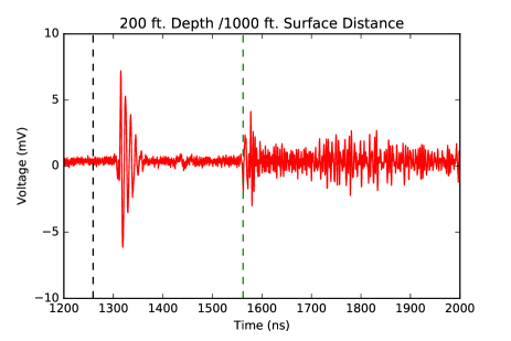
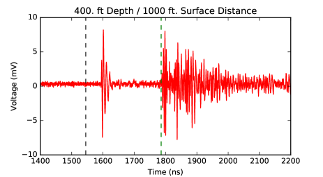
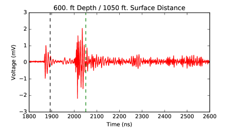
Figure 12: All three waveforms received in the shadowed region after accounting for relative attenuation in the system among measurements. Note that there are two distinct signals, of varying relative amplitudes between the first and second main signal, and there is also significant power seen after the main signals, which was never observed in the non-shadowed region. The black dashed line shows the predicted time of flight of the first pulse and the green dashed line shows the mean predicted time of flight of the second pulse from the FDTD simulations, shown in Table 1. Note that the timescale is double that in Figures 8 and 10. The characteristics that distinguish these signals from those seen in the non-shadowed region (the changes in relative amplitude between the first and second pulse as a function of depth, the signal shape differences between the first and second pulses, and the additional power that follows the second pulse) are directly seen in the FDTD simulations of the shadowed region, shown in Figures 3 and 4.

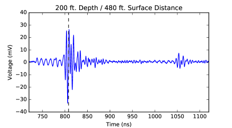
Figure 13: The waveform received for the geometry predicted to be near the edge of the shadowed region. In some firn models it is in the shadowed region and in other models it is in the non-shadowed region. The dashed line shows the predicted time of flight from the FDTD simulations, shown in Table 1. The waveform shape and characteristics are consistent with measurements from the non-shadowed region (see Figure 10), but the amplitude is somewhat suppressed compared to the other measurements in the non-shadowed region.

III.3 Measurements in the Shadowed Region

We also made measurements in three configurations that are shadowed from bulk ray-bending propagation. Figure 12 shows the data from these configurations. Counter to a bulk-propagation-only model, we observe signals in all three configurations in the shadowed region, consistent with previous measurements Barwick et al. (2018) and also consistent with FDTD simulations.

The amplitudes of these signals are uniformly smaller than the signals observed in the non-shadowed region, as shown in Table 2. The waveforms all show a different set of characteristics from those in the non-shadowed region, and are remarkably consistent with the predicted waveforms from the FDTD simulations (see Figures 3 and 4), both in signal shape and in amplitude relative to the non-shadowed region. There are two main pulses seen in all cases in this region, but never seen in the non-shadowed region. The relative amplitude of these two pulses changes as a function of depth, consistent with FDTD simulations. Moreover, the first pulse has a clean signal shape, whereas the second pulse is not as clean, and there is significant power that follows the second pulse for hundreds of nanoseconds. This is also consistent with the behavior observed in the simulations.

In addition to the three measurement configurations that are comfortably in the shadow, there is one measurement configuration that according to the FDTD simulations and the ray tracer resides at the edge of the shadowed region (depending on the firn model parameters one chooses, this configuration either lies inside or outside the shadowed region). The waveform for this configuration is shown in Figure 13. The waveform is consistent in its characteristics with other waveforms in the non-shadowed region, but the amplitude is somewhat suppressed, consistent with FDTD simulations using the model based on the Hawley Hawley et al. (2008) data and the Alley data Alley and Koci (1988).

Although there is no ray-bending bulk propagation ray-tracing solution for these geometries, the surface-wave and horizontal propagation modes Ralston (2005); Barwick et al. (2018) in the ray tracer and the FDTD simulation predict signals in this region. The measured time differences between the first and second pulses are shown in Table 1. These times are consistent with the predictions from FDTD simulations (within 3%), and less so with the ray tracer predictions for horizontal and surface-wave modes.

III.4 Coupling into a Horizontally-Propagating Mode

Bulk Field	Horizontal Tunnel Field	Propagation Loss	Derived Electric Field
Attenuation Length (m)	Attenuation Length (m)		Coupling Fraction
100	100	$1/\sqrt{r}$	$0.09^{+0.42}_{-0.04}$
100	100	$1/r$	$0.15^{+0.46}_{-0.07}$
500	500	$1/\sqrt{r}$	$0.014^{+0.031}_{-0.007}$
500	500	$1/r$	$0.024^{+0.031}_{-0.011}$
1000	1000	$1/\sqrt{r}$	$0.011^{+0.023}_{-0.005}$
1000	1000	$1/r$	$0.019^{+0.017}_{-0.009}$
2000	2000	$1/\sqrt{r}$	$0.010^{+0.020}_{-0.005}$
2000	2000	$1/r$	$0.017^{+0.019}_{-0.008}$
1000	500	$1/\sqrt{r}$	$0.014^{+0.024}_{-0.007}$
1000	500	$\mathbf{1/r}$	$\mathbf{0.023^{+0.023}_{-0.010}}$

Table 4: The calculated electric field coupling fraction under a variety of assumptions, including a choice of $1/r$ or $1/\sqrt{r}$ propagation loss, and various values of the bulk and horizontal tunnel field attenuation lengths. A previous study has determined the bulk field attenuation length at Summit Station to be $\sim 1000$ m Avva et al. (2015), and separate studies at South Pole and Moore’s Bay in Antarctica have shown results consistent with a 500 m field attenuation length and $1/r$ propagation for a horizontal mode Barwick et al. (2018). The row consistent with these previous measurements is highlighted.

For a wave to transition from moving through the bulk medium to propagating along a horizontal or surface-wave mode, power must couple from one mode to the other, rather than continuing the bulk propagation where it would either refract through the surface or reflect off the surface. We can use our data to derive the coupling fraction of power into a horizontally-propagating or surface-wave mode for signals propagating from deep in the ice.

We begin with the calculation of the signal strength for a hypothetical receiver placed 1 m from the transmitter, shown in Table 3. This calculated “system amplitude” depends on the choice of bulk attenuation length. Using this system amplitude for a range of bulk attenuation length choices, and testing a variety of choices of attenuation length for the horizontally-propagating mode (which can in principle be different from the bulk attenuation length) and whether the electric field in the horizontal mode falls as $1/r$ or $1/\sqrt{r}$, we calculate the coupling fraction in each case using the following relationships for the received voltage ($V_{\mathrm{r}}$):

$$V_{\mathrm{r}}=\frac{V_{1\mathrm{m}}\times f\times 1~{}\mathrm{m}}{r_{\mathrm{bulk}}+r_{\mathrm{horiz}}}e^{-r_{\mathrm{bulk}}/l_{\mathrm{bulk}}}\times e^{-r_{\mathrm{horiz}}/l_{\mathrm{horiz}}}$$ (4)

or

$$V_{\mathrm{r}}=\frac{V_{1\mathrm{m}}\times f\times 1~{}\mathrm{m}}{\sqrt{r_{\mathrm{bulk}}}\sqrt{r_{\mathrm{bulk}}+r_{\mathrm{horiz}}}}e^{-r_{\mathrm{bulk}}/l_{\mathrm{bulk}}}\times e^{-r_{\mathrm{horiz}}/l_{\mathrm{horiz}}},$$ (5)

where $V_{1\mathrm{m}}$ is the voltage that would be measured for a receiver at 1 m (shown in Table 3), $f$ is the electric field coupling fraction, $r_{\mathrm{bulk}}$ is the path length of bulk propagation in meters, $r_{\mathrm{horiz}}$ is the path length of horizontal or surface-wave propagation in meters, $l_{\mathrm{bulk}}$ is the field attenuation length for bulk propagation, and $l_{\mathrm{horiz}}$ is the field attenuation length for horizontal or surface-wave propagation. The component of the loss from propagation effects (rather than attenuation) stated in Equations 4 and 5 is not equivalent to taking the scaling factor $1/r$ or $1/\sqrt{r}$ for each segment (bulk and horizontal propagation) and multiplying them together. Simply multiplying the two factors would propagate a signal from a 1 m distance, and then propagate that same signal again from the same 1 m distance, which does not give the correct total scaling factor. Rather, we want to propagate the signal from a 1 m distance to the end of the first leg of the path, and then propagate the remaining signal through the second leg of the path, which results in Equations 4 and 5.

The results for a variety of parameter choices are shown in Table 4. Uncertainties in the Table correspond to the full spread of values obtained if we fit only one of the three measurements at a time. We note that applying a beam pattern correction to the amplitude throughout the analysis reduces the calculated coupling fraction in electric field, but by less than 20% in all cases shown.

Based on previous measurements of bulk attenuation length at Summit Station and of horizontally-propagating modes at South Pole and Moore’s Bay, we choose to highlight the row in Table 4 that shows choices of parameters most consistent with those measurements (a bulk field attenuation length at Summit Station of 1000 m, a horizontally-propagating field attenuation length of 500 m, and a propagation loss of $1/r$ for the horizontal mode). These parameters give a 2.3% coupling fraction in electric field (0.05% in power), with an uncertainty permitting values ranging from 1.3% to 4.6%, representing the full range of values obtained by using only one of the three measurements at a time. For almost all choices of attenuation length, the best-fit coupling fraction in electric field amplitude is 2.4% (0.06% in power) or less to explain the small amplitudes seen in the shadowed region. The only exception is for extremely pessimistic attenuation lengths of 100 m both in the bulk and for the horizontally-propagating mode, which predicts small signal strengths for all signals and has a worse fit to our data in the non-shadowed region. In this case, and assuming $1/r$ propagation, the coupling fraction in electric field is 15% (corresponding to 2.3% in power).

IV Discussion

Although we observe signals in the shadowed region, the amplitudes of these signals are uniformly smaller than those observed in the non-shadowed region, even after accounting for signal path length differences and attenuation. Our data is remarkably consistent with FDTD simulations of the as-measured firn at Summit Station. The measured time of flights are consistent, both in the shadowed and non-shadowed region, with the simulations. The waveform shapes are also consistent, which is especially interesting in the shadowed region. The relative amplitudes predicted by FDTD simulations are also consistent in their order of magnitude. Given the small observed amplitudes in the shadowed region, we find a best-fit electric field coupling fraction of 2.4% or less (0.06% in power), representing the electric field that is coupled into a horizontally-propagating mode, rather than reflected, refracted, or bent. The amplitudes of signals in the shadowed region are shown to be significantly smaller than those in the non-shadowed region, both in the data and in all FDTD simulations.

Knowledge of the relative amplitudes of signals in the shadowed region compared to the non-shadowed region is important for estimating the effective volume of experiments that aim to detect radio emission from neutrinos interacting in glacial ice, since the radio emission from neutrinos would travel at a variety of angles through the firn. Our FDTD simulations show that the exact choice of firn model has significant impact on the exact amplitudes, signal shapes, and signal paths for a certain geometry, especially in the shadowed region. This is not surprising, since propagation in that region (other than surface propagation) arises from density perturbations in the firn, which vary from model to model. This presents a challenge for event reconstruction and volumetric acceptance calculations, especially for near-surface detectors, since the firn near the surface changes most dramatically from year to year and on short distance scales. The relative amplitudes of signals in the shadowed compared to the non-shadowed region could potentially be different at different sites, such as South Pole, which has yet a different set of exact density perturbations in the firn.

The observation of multiple signals (e.g. a surface wave and a bulk-propagation mode in the non-shadowed region or a surface wave and a horizontal mode in the shadowed region) from a single neutrino event would help determine the vertex of the event, relevant for energy and angular reconstruction.

V Acknowledgements

We would like to thank CH2M Hill and the US National Science Foundation (NSF) for the dedicated, knowledgeable, and extremely helpful logistical support team enabling us to perform our work at Summit Station, particularly to J. Jenkins. We are deeply indebted to those who dedicate their careers to help make our science possible in such remote environments. This work was supported by the Kavli Institute for Cosmological Physics at the University of Chicago, Department of Energy Award DE-SC0009937, NSF Award 1752922 and 1607555, the Sloan Foundation, and the Leverhulme Trust. Computing resources were provided by the University of Chicago Research Computing Center.

References

- Arthern et al. (2013) R. J. Arthern et al., Journal of Geophysical Research (Earth Surface) 118, 1257 (2013).
- Koci and Kuivinen (1983) Koci and Kuivinen, Antarctic Journal of the U.S. 18, 113 (1983).
- Avva et al. (2015) J. Avva et al., J. Glaciol. 61, 1005 (2015).
- Barwick et al. (2018) S. W. Barwick et al., (2018), arXiv:1804.10430.
- Hawley et al. (2008) R. L. Hawley, E. M. Morris, and J. McConnell, Journal of Glaciology 54, 839 (2008).
- ARA Collaboration et al. (2012) ARA Collaboration, P. Allison, and et al., Astroparticle Physics 35, 457 (2012).
- Vieregg et al. (2016) A. G. Vieregg, K. Bechtol, and A. Romero-Wolf, J. Cosm. and Astropart. Phys. 2, 005 (2016).
- Alley and Koci (1988) R. Alley and B. Koci, Ann. Glaciol. 10, 1 (1988).
- Alley et al. (1997) R. Alley et al., Journal of Geophysical Research: Oceans 102, 26367 (1997).
- Herron and Langway (1980) M. M. Herron and C. C. Langway, Journal of Glaciology 25, 373 (1980).
- Frezza and Tedeschi (2015) F. Frezza and N. Tedeschi, J. Opt. Soc. Am. A 32, 1485 (2015).
- Ralston (2005) J. P. Ralston, Phys. Rev. D 71, 011503 (2005).
- Besson et al. (2008) D. Z. Besson et al., Astroparticle Physics 29, 130 (2008).
- Alvarez et al. (2015) R. Alvarez et al., (2015), arXiv:1509.04997.
- Kovacs et al. (1995) A. Kovacs, A. Gow, and R. Morey, Cold Regions Science and Technology 23, 245 (1995).
- Taflove and Hagness (2005) A. Taflove and S. Hagness, Computational Electrodynamics: The Finite-Difference Time-Domain Method, 3rd ed. (Artech House, 2005).
- Oskooi et al. (2010) A. F. Oskooi et al., Computer Physics Communications 181, 687 (2010).
- Note (1) Our simulation code is available at https://github.com/cozzyd/iceprop.
- Kravchenko et al. (2003) I. Kravchenko et al., Astroparticle Physics 19, 15 (2003).
- MagGregor et al. (2015) J. A. MagGregor et al., J. Geophys. Res. Earth Surf. 120, 983 (2015).