Disorder correction to the Néel temperature of ruthenium-doped BaFe₂As₂: Theoretical analysis

Abstract

We analyze theoretically nuclear magnetic resonance data for the spin-density wave phase in the ruthenium-doped BaFe₂As₂. Since inhomogeneous distribution of Ru atoms introduces disorder into the system, experimentally observable random spatial variations of the spin-density wave order parameter emerge. Using perturbation theory for the Landau functional, we estimate the disorder-induced correction to the Néel temperature for this material. Calculated correction is significantly smaller than the Néel temperature itself for all experimentally relevant doping levels. This implies that, despite pronounced spatial non-uniformity of the order parameter, the Néel temperature is quite insensitive to the disorder created by the dopants.

I Introduction

In this paper we discuss the influence of doping-induced disorder on the Néel temperature of the ruthenium-doped BaFe₂As₂. The compound is a representative of a wide class of pnictide superconductors, actively studied in the last decade. Many members of this class, including BaFe₂As₂ itself, experience a transition into a spin-density wave (SDW) phase. The Néel temperature for this transition is sensitive to the doping concentration and decreases monotonically when the doping grows. Beyond certain doping level ($\sim 25$% for Ru-doped BaFe₂As₂) the magnetism is completely replaced by the superconducting phase.

Although doping by ruthenium atoms is an important experimental method Thaler et al. (2010); Dhaka et al. (2011); Ma et al. (2012); Zhao et al. (2013) to explore electronic correlation effects in BaFe₂As₂, introduction of dopants unavoidably produces crystal imperfections Wang et al. (2013); Ye et al. (2014); Reticcioli et al. (2017). While disorder might be a source Prozorov et al. (2014) of interesting phenomena, it is often an undesirable factor blurring or masking an investigated feature. This concern is quite general for doped iron-based superconductors. Indeed, the presence of imperfections in this family of superconducting materials is well-documented: inhomogeneities of the charge density were observed experimentally Park et al. (2009); Inosov et al. (2009); Lang et al. (2010); Bonville et al. (2010); Shen et al. (2011); Bernhard et al. (2012); Civardi et al. (2016) and discussed theoretically Sboychakov et al. (2013); de’ Medici (2017) in several publications.

For an imperfect system, it is reasonable to ask to what extent a particular physical property is affected by the disorder. Depending on the nature of the physical property under consideration, the answer to this question may differ. For instance, NMR measurements Laplace et al. (2012) for BaFe₂As₂ are consistent with the notion that the SDW order parameter varies markedly over the sample volume. At the same time, our theoretical analysis of the same data shows that, notwithstanding pronounced non-uniformity of the ordered state, the Néel temperature $T_{\rm N}$ is fairly insensitive to the dopant-induced inhomogeneities.

Our analysis is based on the perturbation theory Larkin and Ovchinnikov (1972) in powers of the disorder strength. A key ingredient of our study is a phenomenological model for disorder distribution, developed in Ref. Laplace et al., 2012 to interpret the NMR data. The correction to the Néel temperature is estimated within the Landau functional framework and is determined to be small. This finding is the main result of our work. It implies that $T_{\rm N}$ can be reliably calculated, at least in principle, using disorder-free models, and the Néel temperature can act as a benchmark characteristic, useful for checking the validity of theoretical conclusions.

The paper is organized as follows. In Sec. II the model is introduced. The perturbation theory calculations are performed in Sec. III. They are applied to the analysis of the data in Sec. IV. Section V contains the discussion and conclusions. Some auxiliary derivations are presented in Appendix.

II Model

Our analysis is based on experimental findings of Ref. Laplace et al., 2012, which performed NMR studies of the SDW transition in ruthenium-doped BaFe₂As₂. Since ruthenium substitutes iron atoms, chemical formula for the resultant alloy is Ba(Fe_1-xRu_x)₂As₂, where the doping concentration $x$ changes in a wide range $0<x<1$. Since Ru is isovalent to Fe, it is believed Laplace et al. (2012) that doping by ruthenium atoms creates milder modifications to the electron structure of the compound as compared, for example, with doping by cobalt atoms. In particular, one may expect that Ru substitution does not generates significant de-nesting, since no electrons are introduced due to dopants. Yet, Ru doping weakens the SDW phase: the Néel temperature decreases as a function of doping, until the SDW is replaced by the superconductivity above $\sim 0.3$.

For our study we need to calculate correction to the SDW transition temperature, which turns out to be small. Consequently, the Landau free energy functional

$$F[S({\bf r})]=\int\left\{C_{\|}\left[\left(\nabla_{x}S\right)^{2}+\left(\nabla_{y}S\right)^{2}\right]+C_{\perp}\left(\nabla_{z}S\right)^{2}\right.$$ (1)

$$\left.+AS^{2}+\frac{B}{2}S^{4}\right\}d^{3}{\bf r},$$

describing the material’s behavior near the transition, can be justifiably used. In Eq. (1), symbol $S=S({\bf r})$ is the SDW magnetization, which plays the role of the order parameter. While, in general, the magnetization is a vector, for our purposes it is sufficient to treat $S$ as a scalar. Coefficients $C_{\|}$, $C_{\perp}$, and $B$ are all positive. To account for the quasi-two-dimensional (Q2D) anisotropy present in the pnictides the coefficients $C_{\|}$ and $C_{\perp}$ must satisfy the inequality $C_{\|}\gg C_{\perp}$. We will make this condition more specific below.

For the coefficient $A$, we assume that it is spatially inhomogeneous: $A=A({\bf r})$. A convenient parametrisation for $A({\bf r})$ is as follows

$$A({\bf r})=a[T-T_{\rm N}-\delta T_{\rm N}({\bf r})],\quad a>0,$$ (2)

where $T$ is the system temperature, the disorder-averaged Néel temperature is $T_{\rm N}$. Local variation of the Néel temperature $\delta T_{\rm N}({\bf r})$ satisfies

$$\langle\delta T_{\rm N}({\bf r})\rangle\equiv 0.$$ (3)

Here triangular brackets $\langle\ldots\rangle$ denote the average over disorder configurations.

Formulating this model, we assumed that the doping-induced disorder affects the system mostly through the spatial variation of $\delta T_{\rm N}({\bf r})$. Inhomogeneities of $C_{\|,\perp}$ and $B$ are much less important, for they contribute to the subleading corrections. Therefore, we will treat these parameters as if they are independent of ${\bf r}$.

Variation of $F$ over $S$ gives us the following equation for the order parameter $S$

$$-\left[\xi_{\|}^{2}\left(\nabla_{x}^{2}+\nabla_{y}^{2}\right)+\xi_{z}^{2}\nabla_{z}^{2}\right]S-\delta t({\bf r})S+bS^{3}=-tS,$$ (4)

where coefficient $b$ equals to $b=B/(aT_{\rm N})$, the dimensionful parameter $\xi_{\|}^{2}=C_{\|}/\left(aT_{\rm N}\right)$ is the in-plane correlation length, $\xi_{z}^{2}=C_{\perp}/\left(aT_{\rm N}\right)$ is the transverse correlation length. Dimensionless variation of the local Néel temperature $\delta t$ and dimensionless temperature $t$ in Eq. (4) are

$$\delta t({\bf r})=\frac{\delta T_{\rm N}\left({\bf r}\right)}{T_{\rm N}},\quad t=\frac{T-T_{\rm N}}{T_{\rm N}}.$$ (5)

We want to calculate the lowest (second) order correction $\Delta T_{\rm N}$ to the Néel temperature $T_{\rm N}$ caused by disorder $\delta T_{\rm N}({\bf r})$. Of course, once $\Delta T_{\rm N}$ is evaluated, the experimentally measurable transition temperature is determined as $T_{\rm N}+\Delta T_{\rm N}$. To find $\Delta T_{\rm N}$ we need to study only the linear part of Eq. (4). Intuitively, one may argue that, since $O(|S|^{3})$ term in Eq. (4) is much smaller than $O(|S|)$ near the transition temperature, $O(|S|^{3})$ term may be omitted. A more precise line of reasoning is based on the realization that the transition temperature is controlled by the bilinear part of the Landau functional: as long as the bilinear form remains positive-definite, the disordered phase ($S\equiv 0$) remains stable. At the transition temperature the lowest eigenvalue of the bilinear form vanishes (that is, the bilinear form becomes non-negative-definite). Thus, to calculate the transition temperature, we need to study the following eigenvalue equation

$$-\left[\xi_{\|}^{2}\left(\nabla_{x}^{2}+\nabla_{y}^{2}\right)+\xi_{z}^{2}\nabla_{z}^{2}\right]S-\delta t({\bf r})S=-t_{\rm N}S.$$ (6)

Physical meaning of parameter $t_{\rm N}$ is the dimensionless disorder-induced correction to the transition temperature:

$$\Delta T_{\rm N}=T_{\rm N}t_{\rm N}.$$ (7)

Mathematically, the value of $-t_{\rm N}$ is the lowest eigenvalue of the linear operator in the left-hand side of Eq. (6). Once this eigenvalue is known, relation (7) can be used to find the dimensionful correction.

III Calculations

Before starting the calculations of $t_{\rm N}$, it is useful to observe that Eq. (6) is similar to Schrödinger equation. This analogy allows us to determine the correction to the Néel temperature using a familiar language of the perturbation theory for a Schrödinger operator. Within this analogy, the quantity $-\delta t({\bf r})$ plays the role of small perturbation in potential energy, and $-t_{\rm N}$ is the correction to the lowest eigenvalue of the non-perturbed Hamiltonian.

For the three-dimensional systems, the perturbative derivation of $t_{\rm N}$ has been reported in Ref. Larkin and Ovchinnikov, 1972. Since the pnictides are layers systems, they are often described by two-dimensional or Q2D models. Our main goal in this Section is to adapt the calculations of Ref. Larkin and Ovchinnikov, 1972 to a quasi-two-dimensional system. While our discussion is, in many respects, similar to the three-dimensional case, yet, certain technical points require more delicate treatment.

Let us start with the calculations. Using the logic of the perturbation theory for the Schrödinger operator, we will find the correction to the ground state eigenvalue for the unperturbed operator

$$H_{0}=-\left[\xi_{\|}^{2}\left(\nabla_{x}^{2}+\nabla_{y}^{2}\right)+\xi_{z}^{2}\nabla_{z}^{2}\right].$$ (8)

The unperturbed ground state is equal to

$$S^{(0)}=\frac{1}{\sqrt{V}},$$ (9)

where $V$ is the volume of the sample. The first-order correction to order parameter $S^{(1)}$ satisfies the equation

$$\left[\xi_{\|}^{2}\left(\nabla_{x}^{2}+\nabla_{y}^{2}\right)+\xi_{z}^{2}\nabla_{z}^{2}\right]\!S^{(1)}+\frac{\delta t({\bf r})}{\sqrt{V}}=\frac{t^{(1)}_{\rm N}}{\sqrt{V}}.$$ (10)

Here $t^{(1)}_{\rm N}$ is the first-order correction to the eigenvalue $t_{\rm N}$.

Averaging this equation over the disorder, we derive, using Eq. (3), that

$$\left[\xi_{\|}^{2}\left(\nabla_{x}^{2}+\nabla_{y}^{2}\right)+\xi_{z}^{2}\nabla_{z}^{2}\right]\langle S^{(1)}\rangle=\frac{1}{\sqrt{V}}t^{(1)}_{\rm N}.$$ (11)

Since $\langle S^{(1)}\rangle$ is independent of ${\bf r}$, we have $\nabla\langle S^{(1)}\rangle\equiv 0$. Therefore,

$$t^{(1)}_{\rm N}=0.$$ (12)

Substituting this result into Eq. (10), we calculate the first-order correction to order parameter

$$S^{(1)}({\bf r})=\frac{1}{\sqrt{V}}\int G({\bf r}-{\bf r^{\prime}})\,\delta t({\bf r^{\prime}})d^{3}{\bf r^{\prime}}.$$ (13)

In this relation $G({\bf r})$ is the Green’s function of the operator $H_{0}$, Eq. (8):

$$G({\bf r})=\int\!\frac{d^{3}{\bf k}}{(2\pi)^{3}}\frac{e^{i{\bf k}{\bf r}}}{\xi_{\|}^{2}\left(k_{x}^{2}+k_{y}^{2}\right)+\xi_{z}^{2}k_{z}^{2}}.$$ (14)

Fourier transform of $G({\bf r})$ equals to

$$G_{\bf k}=\frac{1}{\xi_{\|}^{2}\left(k_{x}^{2}+k_{y}^{2}\right)+\xi_{z}^{2}k_{z}^{2}}.$$ (15)

To find the second-order correction to $t_{\rm N}$ it is necessary to obtain the equation for the second-order correction to order parameter $S^{(2)}$. Retaining all terms up to the second order in $\delta t$, we can write

$$\left[\xi_{\|}^{2}\left(\nabla_{x}^{2}+\nabla_{y}^{2}\right)+\xi_{z}^{2}\nabla_{z}^{2}\right]\left(S^{(0)}+S^{(1)}+S^{(2)}\right)+$$ (16)

$$+\delta t\left(S^{(0)}+S^{(1)}\right)=t^{(2)}_{\rm N}S^{(0)}.$$

Collecting all second-order terms in this expression, it is possible to derive for $t^{(2)}_{\rm N}$:

$$t^{(2)}_{\rm N}=\int\!S^{(0)}\left[\xi_{\|}^{2}\left(\nabla_{x}^{2}+\nabla_{y}^{2}\right)+\xi_{z}^{2}\nabla_{z}^{2}\right]S^{(2)}({\bf r})d^{3}{\bf r}+$$ (17)

$$+\int\!\delta t({\bf r})S^{(0)}S^{(1)}({\bf r})d^{3}{\bf r}.$$

Since $S^{(0)}$ is independent of ${\bf r}$, the first term can be written as a divergence of some vector field. Therefore, the volume integral can be replaced with a surface integral, which vanishes for periodic boundary conditions. Thus

$$t^{(2)}_{\rm N} = \int\!\delta t({\bf r})S^{(0)}S^{(1)}({\bf r})d^{3}{\bf r}$$

$$= \frac{1}{V}\int\!\delta t({\bf r})\delta t({\bf r}^{\prime})G({\bf r}-{\bf r}^{\prime})d^{3}{\bf r}\,d^{3}{\bf r}^{\prime}.$$

This equation explicitly demonstrates that the correction $t^{(2)}_{\rm N}$ is a random quantity, a (bilinear) functional of the disorder configuration $\delta t$. However, we prove in Appendix A that the dispersion of $t^{(2)}_{\rm N}$ vanishes in the thermodynamic limit. Thus, since $\langle t^{(2)}_{\rm N}\rangle\approx t^{(2)}_{\rm N}$, it is permissible to work with the average value of $t^{(2)}_{\rm N}$. Once the disorder averaging in Eq. (17) is performed, we obtain

$$\langle t^{(2)}_{\rm N}\rangle = \frac{1}{V}\int\!\langle\delta t({\bf r})\,\delta t({\bf r}^{\prime})\rangle G({\bf r}-{\bf r^{\prime}})\,d^{3}{\bf r}\,d^{3}{\bf r}^{\prime}$$

$$= \int\!\tau({\bf r})G({\bf r})\,d^{3}{\bf r}.$$

Below we will assume that the disorder correlation function

$$\tau({\bf r}-{\bf r^{\prime}})=\langle\delta t({\bf r})\,\delta t({\bf r}^{\prime})\rangle$$ (20)

has the following structure

$$\tau({\bf r})=\langle\Delta t^{2}\rangle\exp\left(-\frac{x^{2}+y^{2}}{2r_{0}^{2}}\right)\delta\left(\frac{z}{s}\right).$$ (21)

In this expression, $\langle\Delta t^{2}\rangle$ is the variance of the local dimensionless Néel temperature, $s$ is the distance between Fe layers, $r_{0}$ is the disorder correlation length in a single Fe layer. The distribution of the Ru atoms in neighboring layers is assumed to be uncorrelated. This feature is captured by $\delta(z/s)$ in Eq. (21).

Switching in Eq. (III) from integration over real space to integration over momentum space, we find Larkin and Ovchinnikov (1972)

$$\langle t^{(2)}_{\rm N}\rangle=\int\!\frac{d^{3}{\bf k}}{(2\pi)^{3}}\tau_{\bf k}G_{\bf k},$$ (22)

where the Fourier transform of the correlation function $\tau({\bf r})$ is

$$\tau_{\bf k}=2\pi\langle\Delta t^{2}\rangle r_{0}^{2}s\,\exp\!\left[-\frac{r_{0}^{2}}{2}\left(k_{x}^{2}+k_{y}^{2}\right)\right].$$ (23)

Equation (22), with the help of Eqs. (15) and (23), can be re-written as

$$\langle t^{(2)}_{\rm N}\rangle=\frac{\langle\Delta t^{2}\rangle r_{0}^{2}s}{(2\pi)^{2}}\int\!d^{3}{\bf k}\frac{\exp\left(-\left(k_{x}^{2}+k_{y}^{2}\right)r_{0}^{2}/2\right)}{\xi_{\|}^{2}\left(k_{x}^{2}+k_{y}^{2}\right)+\xi_{z}^{2}k_{z}^{2}}.$$ (24)

Here the integration over $k_{x}$ and $k_{y}$ is performed from $-\infty$ to $\infty$. At the same time, the integration over $k_{z}$ is from $-\pi/s$ to $\pi/s$. Taking this into account we obtain

$$\!\left<t^{(2)}_{\rm N}\right>=\frac{\langle\Delta t^{2}\rangle r_{0}^{2}s}{4\pi}\!\int\limits_{0}^{\infty}\!dk_{\|}^{2}\int\limits_{-\pi/s}^{\pi/s}\!dk_{z}\frac{\exp\left(-k_{\|}^{2}r_{0}^{2}/2\right)}{\xi_{\|}^{2}k_{\|}^{2}+\xi_{z}^{2}k_{z}^{2}},$$ (25)

where $k_{\|}^{2}=k_{x}^{2}+k_{y}^{2}$. It is important to note that the correction is infinite for two-dimensional systems. Indeed, the integral in Eq. (25) diverges logarithmically in the limit $\xi_{z}=0$. To regularize the integral we evaluate it at finite $\xi_{z}$, that is, in Q2D setting. First of all, we denote $q=k_{\|}^{2}r_{0}^{2}$, $\alpha=\xi_{z}/s$, $\beta=\xi_{\|}/r_{0}$, $k_{z}s=u$ and integrate last equation over $q$ by parts:

$$\!\langle t^{(2)}_{\rm N}\rangle=\frac{\langle\Delta t^{2}\rangle}{4\pi\beta^{2}}\!\int_{-\pi}^{\pi}du\int_{0}^{\infty}\!dq\frac{\exp\left(-\frac{q}{2}\right)}{\left[q+\alpha^{2}u^{2}/\beta^{2}\right]}=$$ (26)

$$=-\frac{\langle\Delta t^{2}\rangle}{4\pi\beta^{2}}\!\int_{-\pi}^{\pi}du\ln\left(0.89\frac{\alpha^{2}u^{2}}{\beta^{2}}\right)\left[1+O\left(\frac{\alpha^{2}u^{2}}{\beta^{2}}\right)\right].$$

Here we assume that $\alpha^{2}\pi^{2}/\beta^{2}\ll 1$. This condition will be discussed in subsection V.3.

Returning to the evaluation of $\langle t^{(2)}_{\rm N}\rangle$, we perform the integration over $u$:

$$\langle t^{(2)}_{\rm N}\rangle\approx\frac{\langle\Delta t^{2}\rangle}{\beta^{2}}\left[1-\ln\left(0.94\frac{\pi\alpha}{\beta}\right)\right].$$ (27)

For the logarithmic function in this expression we expect, as usual, that its value is of the order of unity. Thus

$$\langle t^{(2)}_{\rm N}\rangle\sim\frac{\langle\Delta t^{2}\rangle}{\beta^{2}}=\frac{r_{0}^{2}}{\xi_{\|}^{2}}\langle\Delta t^{2}\rangle.$$ (28)

Thus, the second-order correction to dimensionless Néel temperature (28) depends on the variance of the local dimensionless Néel temperature and on the ratio of the in-plane length $\xi_{\|}$ and disorder correlation length in a single Fe layer $r_{0}$. As for the interlayer parameters $s$ and $\xi_{z}$, they introduce weak logarithmic correction to the main result. This correction was neglected in Eq. (28).

Obviously, Eq. (28) is applicable not only for antiferromagnets, but also for superconductors, as well as other ordered phases. As a specific application, in the next section we will use this formula to find the corrections to the Néel temperature of doped BaFe₂As₂.

IV Analysis of experimental data

In this section we will apply Eq. (28) to the analysis of the data published in Ref. Laplace et al., 2012. This paper is of particular interest for us here, since it discusses statistical properties of the local Néel temperature $\delta T_{\rm N}({\bf r})$ for doped BaFe₂As₂. Namely, the authors of Ref. Laplace et al., 2012 have concluded that their data is consistent with the assumption that $\delta T_{\rm N}({\bf r})$ is obtained by coarse-graining of the random dopant distribution over small, but finite, patches of the underlying two-dimensional lattice. The model for $\delta T_{\rm N}({\bf r})$ is formulated Laplace et al. (2012) in the following manner. Initially, the whole two-dimensional lattice of a Fe layer is split into square patches. The size of each patch is $4\times 4$ unit cells (obviously, a patch contains $N=16$ unit cells). For a particular distribution of Ru atoms over a layer, one defines a function $n({\bf r})$, which is a number of Ru atoms within a patch located at ${\bf r}$. As a result, the local coarse-grained doping $x_{\rm loc}({\bf r})=n({\bf r})/N$ is introduced. Disorder-average of this function is equal to the average doping:

$$\langle x_{\rm loc}({\bf r})\rangle=x.$$ (29)

Function $x_{\rm loc}({\bf r})$ is used to determine local variation of the Néel temperature according to the rule

$$\delta T_{\rm N}({\bf r})=T_{\rm N}(x_{\rm loc}({\bf r}))-\langle T_{\rm N}(x_{\rm loc}({\bf r}))\rangle,$$ (30)

where the dependence of the Néel temperature $T_{\rm N}=T_{\rm N}(x)$ on the average doping $x$ is directly measured experimentally. We find that the linear fit

$$T_{\rm N}(x)=T_{\rm N}^{0}(1-\gamma x),\text{\ where\ }T_{\rm N}^{0}=140\,{\rm K},\ \gamma=2,$$ (31)

accurately describes the data. Table 1 attests to the quality of this approximation. Formula (31) works well in the interval $0<x<0.2$. For larger doping levels, the Néel temperature is expected to decrease faster than described by Eq. (31). (Therefore, our results will gradually become less accurate when $x$ grows beyond 0.2.)

The outlined disorder model allows us to obtain both $r_{0}$ and $\langle\Delta t^{2}\rangle$ for our Eq. (28). Mathematically speaking, the patch size corresponds to the correlation length $r_{0}$ in Eq. (21). Indeed, if $|{\bf r}-{\bf r}^{\prime}|>r_{0}$, the random quantities $\delta T_{\rm N}({\bf r})$ and $\delta T_{\rm N}({\bf r}^{\prime})$ characterize different patches. Consequently, they are uncorrelated, which means that $\langle t({\bf r})t({\bf r}^{\prime})\rangle\approx 0$, in agreement with Eq. (21). Therefore, we can write

$$r_{0}\approx 4a_{0}\approx 11\,{\rm\AA},$$ (32)

where $a_{0}\approx 2.8$ Å is the unit cell size, see Ref. Thaler et al., 2010. Consistent with Ref. Laplace et al., 2012, we assume that the in-layer cell is defined in such a manner that there is one iron atom per cell.

	$x=0.00$	$x=0.05$	$x=0.15$	$x=0.20$	$x=0.25$
$T_{\rm N}(x)$, K,	135	130	95	80	55
Ref. Laplace et al.,2012
$T_{\rm N}(x)$, K,	140	126	98	84	70
Eq (31)
$\Delta T_{\rm N}(x)$, K,	0	3.3	6.9	7.4	7.2
Eq (41)

Table 1: Experimentally measured Néel temperature (from Ref. Laplace et al., 2012), analytical fit to this temperature, see Eq. (31), and disorder-induced correction to the transition temperature, Eq. (41), for several doping concentrations $x$. The values of $x$ from this table correspond to the experimentally studied samples, Ref. Laplace et al., 2012. The presented data shows that the fit (31) works well for $x\leq 0.2$. Only when $x=0.25$, significant discrepancy between the measured and fitted Néel temperatures emerges. Correction $\Delta T_{\rm N}$ remains small (ratio $\Delta T_{\rm N}/T_{\rm N}$ remains of the order of 10% or less) for all $x$.

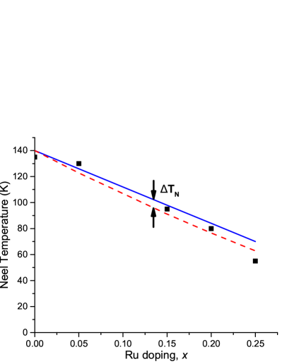
Figure 1: Néel temperature for Ru-doped BaFe₂As₂ versus doping $x$. Experimental values of the Néel temperature $T_{\rm N}(x)$ are shown here as black squares. The data is approximated by solid (blue) straight line, see Eq. (31). The Néel temperature for a doped sample without any disorder is depicted by dashed (red) curve. The disorder-induced correction to the Néel temperature is represented by the difference between the solid and dashed curves. It is estimated using Eq. (41).

Quantity $\langle\Delta t^{2}\rangle=\langle[\delta t({\bf r})]^{2}\rangle$ is the variance of $\delta t$ within a single patch. It can be calculated as follows. Combining Eq. (5) Eq. (30) and (31) we write:

$$\delta t({\bf r})=\frac{N-\gamma n({\bf r})}{N-\gamma n}-1=\frac{\gamma\left(n-n({\bf r})\right)}{N-\gamma n},$$ (33)

where $n=Nx$ is the average number of impurities in a patch. The variance of $\delta t$ within a single patch is

$$\langle\Delta t^{2}\rangle=\frac{\gamma^{2}\langle\Delta n^{2}\rangle}{\left(N-\gamma n\right)^{2}},\quad\text{where}\quad\Delta n=n({\bf r})-n.$$ (34)

This equation reduces the task of calculating $\langle\Delta t^{2}\rangle$ to the calculation of $\langle\Delta n^{2}\rangle$. (The latter average will be fond below with the help of the outlined disorder model.) Such a simple relation between the two is a consequence of linear dependence of $T_{\rm N}$ on doping $x$. In principle, to improve agreement with the experimental data, one can introduce non-linear terms to Eq. (31). However, we expect that this modification does not significantly change final results, but only complicates calculations. To keep our formalism simple and intuitively clear, we always use Eq. (31) in our study.

Quantity $\langle\Delta n^{2}\rangle$ characterizes the distribution of impurities within a single patch. It can be easily estimated as follows. The number of impurities in a patch $n({\bf r})$ is a random quantity with the binomial distribution. Its number of “attempts” coincides with the number of unit cells inside a patch: $N=16$. The distribution is characterized by “success probability” $p=n/N=x$ (this is the probability of finding a Ru atom at a given unit cell inside the patch). For the binomial distribution with these parameters the answer is $\langle\Delta n^{2}\rangle=Np(1-p)=n(N-n)/N$. Substituting this relation into Eq. (34), we find

$$\langle\Delta t^{2}\rangle=\frac{\gamma^{2}n(N-n)}{N\left(N-\gamma n\right)^{2}}.$$ (35)

Using Eq. (28) and Eq. (35) we determine the correction to dimensionless Néel temperature

$$\langle t^{(2)}_{\rm N}\rangle\thickapprox\frac{r_{0}^{2}\gamma^{2}n(N-n)}{N\xi_{\|}^{2}\left(N-\gamma n\right)^{2}}.$$ (36)

The dimensionful correction to Néel temperature can be found with the help of Eq. (7)

$$\Delta T_{\rm N}=\langle t^{(2)}_{\rm N}\rangle T_{\rm N}^{0}\left(1-\gamma\frac{n}{N}\right)\thickapprox\frac{r_{0}^{2}\gamma^{2}n(N-n)}{\xi_{\|}^{2}N^{2}\left(N-\gamma n\right)}T_{\rm N}^{0},$$ (37)

or, with estimate Eq. (32), it is equivalent to

$$\Delta T_{\rm N}\thickapprox\frac{a_{0}^{2}\gamma^{2}x(1-x)}{\xi_{\|}^{2}\left(1-\gamma x\right)}T_{\rm N}^{0}.$$ (38)

To calculate this correction, the last quantity we need to find is $\xi_{\|}$. We estimate $\xi_{\|}$ from the microscopic BCS-like theory: $\xi_{\|}\approx 0.13{v_{\rm F}}/{T_{\rm N}}$, where $v_{\rm F}$ is the Fermi velocity. This equation is valid provided that the system’s ordered phase is of mean field BCS character. For more details, one may consult standard textbook, such as Refs. de Gennes, 1996; White and Geballe, 1984. Thus, we can write

$$\xi_{\|}(x)\approx\frac{0.13\,v_{\rm F}}{T_{\rm N}^{0}(1-\gamma x)},$$ (39)

where experimentally measured Dhaka et al. (2011) value of the Fermi velocity for the compound is virtually doping-independent and equal to $v_{\rm F}\sim 0.7$ eVÅ.

Finally, combining Eqs. (38) and (39), we find

$$\Delta T_{\rm N}\thickapprox\frac{a_{0}^{2}\gamma^{2}x(1-x)\left(1-\gamma x\right)}{(0.13v_{\rm F})^{2}}(T_{\rm N}^{0})^{3}.$$ (40)

Once all constants are substituted, equation for the correction to the Néel temperature reads:

$$\Delta T_{\rm N}\thickapprox 77x(1-x)\left(1-2x\right).$$ (41)

This correction is calculated for several concentrations of Ru atoms, see Table 1. The values of $x$ from the Table correspond to the doping levels of the samples studied in Ref. Laplace et al., 2012. We see that the correction is quite small for $x<0.2$. Figure 1 offers additional illustration to this conclusion. Beyond doping $\sim 0.2$ the system quickly becomes superconducting. Thus, for most of the doping range where the SDW exists, the disorder-induced corrections to the Néel temperature remain weak.

V Discussion

V.1 Relevance for other compounds

The presented calculations are simple and intuitively clear. They also convey a useful piece of information about BaFe₂As₂. One might inquire if other compounds can be analyzed in a similar manner.

Our procedure depends crucially on the fact that Ru atoms are isovalent with iron atoms which Ru atoms substitute. Consequently, the doping does not introduce significant modifications to the electronic structure of the material Dhaka et al. (2011). This allows us to write the simplest Landau functional (1), which remains applicable as long as the Fermi surface nesting is maintained. For different choice of the dopants, the doping may act to erode nesting, causing significant modifications to the structure of functional (1). In this situation, it becomes difficult to justify our model in its present form. Thus, we must limit ourselves by materials with isovalent doping.

For isovalent doping, Eq. (28) is valid, and can be used to estimate the disorder-induced correction. This equation, of course, requires a practical model of disorder in the material. The model cannot be obtained by theoretical means, and must be supplied by experiment. For the very least, parameters $r_{0}$ and $\langle\Delta t^{2}\rangle$ must be known. Obviously, Ref. Laplace et al., 2012 fulfills these requirements for BaFe₂As₂. Execution of the similar experimental studies to other pnictide superconductors may bring useful results about the role of the disorder in these materials.

V.2 Comparison of $\xi_{\|}$ and $r_{0}$

Equation (39) allows us to estimate $\xi_{\|}$ for different values of $x$. We determine that $\xi_{\|}$ varies between $7.5$ Å at $x=0$ to $15$ Å at $x=0.25$. The disorder correlation length $r_{0}$, introduced and discussed in Sections III and IV, is of the same order:

$$\xi_{\|}\sim r_{0},$$ (42)

see estimate (32). This relation is not a coincidence, and can be explained as follows. Purely local functional (1) is an approximation to a more complicated functional with a non-local kernel. The kernel is spread over a finite size, which we denote $\xi_{\|}$. (When the system obeys the BCS theory, the kernel may be explicitly evaluated, see, for example, Chapter 7 of the de Gennes book de Gennes (1996). However, we expect that the non-local functional itself, as well as the scale $\xi_{\|}$, are well-defined concepts, even when the BCS microscopic theory is inapplicable.) To determine the free energy density at a given point ${\bf R}$, such a functional averages the system’s properties over a circle of radius $\xi_{\|}$ centered at ${\bf R}$. For smooth variation of $S({\bf r})$, the non-local functional may be replaced by purely local Eq. (1). Within this simplified formalism, the length scale $\xi_{\|}$ emerges as a coefficient in front of the derivatives in Eq. (4). This argument implies that the parameter $\xi_{\|}$ describes the smallest length scale below which the functional (1) is undefined, and any fragment of the lattice of size $\xi_{\|}$ must be treated as a single unit. This gives an obvious explanation to the fact that the NMR experimental data Laplace et al. (2012) was best fitted under the assumption that the doping-introduced disorder should be averaged over finite-size patches. Our reasoning naturally equates the size of these patches $r_{0}$ and parameter $\xi_{\|}$.

V.3 The role of the anisotropy

Evaluating integral in Eq. (26) we imposed the following restriction $\pi^{2}\alpha^{2}/\beta^{2}\ll 1$. It implies that the Landau functional coefficients should satisfy ${C_{\|}}/{C_{\perp}}\gg{\pi^{2}r_{0}^{2}}/{s^{2}}$. Since BaFe₂As₂ has two layers per one unit cell, the interlayer distance $s$ equals to $s=c_{0}/2\approx 6.5$Å, where $c_{0}$ is the $c$-axis lattice constant (crystallographic data for BaFe₂As₂ may be found in Ref. Thaler et al., 2010). Using Eq. (32), we derive ${C_{\|}}/{C_{\perp}}\gg 30$. This means that, for Eq. (27) to be valid, the Landau functional must be sufficiently anisotropic. It is not immediately obvious how to estimate the anisotropy of the coefficients $C_{\perp}$, $C_{\|}$ for BaFe₂As₂. Fortunately, the importance of this condition is not too crucial. Indeed, even in a perfectly isotropic system the estimate (28) remains valid up to a numerical factor Larkin and Ovchinnikov (1972).

V.4 Conclusions

In this paper, we studied the correction to the Néel temperature introduced by the inhomogeneities of the doping atoms distribution for Ru-doped BaFe₂As₂. Using perturbation theory, we expressed the lowest-order correction to the Néel temperature of a Q2D system in terms of the disorder distribution properties. Previously developed phenomenological model for the disorder in Ru-doped BaFe₂As₂ allows us to complete the calculations. The corrections are found to be quite small for all doping levels where the material experiences the SDW transition. This suggests that the Néel temperature in Ru-doped BaFe₂As₂ may be studied using spatially homogeneous models.

Appendix A Dispersion of the second correction $t^{(2)}_{\rm N}$

In this Appendix we demonstrate that the dispersion of $t^{(2)}_{\rm N}$, given by Eq. (III), vanishes in the thermodynamic limit. Namely, we intend to prove that the disorder average of $D$, where

$$D=[t^{(2)}_{\rm N}-\langle t^{(2)}_{\rm N}\rangle]^{2},$$ (43)

is small for large systems. Since

$$\langle D\rangle=\langle[t^{(2)}_{\rm N}]^{2}\rangle-\langle t^{(2)}_{\rm N}\rangle^{2},$$ (44)

we need to evaluate $\langle[t^{(2)}_{\rm N}]^{2}\rangle$. The random quantity $[t^{(2)}_{\rm N}]^{2}$ can be expressed as

$$[t^{(2)}_{\rm N}]^{2}=\frac{1}{V^{2}}\int\delta t({\bf r})\delta t({\bf r^{\prime}})G({\bf r-r^{\prime}})d^{3}{\bf r}d^{3}{\bf r^{\prime}}\int\delta t({\bf r^{\prime\prime}})\delta t({\bf r^{\prime\prime\prime}})G({\bf r^{\prime\prime}-r^{\prime\prime\prime}})d^{3}{\bf r^{\prime\prime}}d^{3}{\bf r^{\prime\prime\prime}}.$$ (45)

In this equation, the Green’s function $G$ is given by Eq. (14).

Figure 2: Illustration to the expansion Eq. (A). Locality requires that the average $\left\langle\delta t({\bf r})\delta t({\bf r^{\prime}})\delta t({\bf r^{\prime\prime}})\delta t({\bf r^{\prime\prime\prime}})\right\rangle$ vanishes unless even number of points lie within a radius $r_{0}$ from each other. Thus, the configurations shown in panels (c) and (d) correspond to vanishing $\langle\delta t\delta t\delta t\delta t\rangle$. Panel (a), on the other hand, represents the first term on the right-hand side of Eq. (A). Two other terms are obtained by permutations of ${\bf r},\ldots,{\bf r}^{\prime\prime\prime}$. Panel (b) also corresponds to finite average. However, because of the constraint, requiring all four points be confined within a distance $\sim r_{0}$, after integration over space in Eq. (45), one obtains a contribution which, in the thermodynamic limit, is much smaller than that of panel (a).

As one can see from Eq. (45), to evaluate $\langle[t^{(2)}_{\rm N}]^{2}\rangle$ we must determine the four-point disorder correlation function

$$\tau^{(4)}({\bf r},{\bf r^{\prime}},{\bf r^{\prime\prime}},{\bf r^{\prime\prime\prime}})=\langle\delta t({\bf r})\delta t({\bf r^{\prime}})\delta t({\bf r^{\prime\prime}})\delta t({\bf r^{\prime\prime\prime}})\rangle.$$ (46)

Below, for simplicity, we will assume that the disorder correlation function is isotropic. Strictly speaking, this assumption is inapplicable for pnictide compounds, and our choice for the disorder correlation function, Eq. (21), is explicitly anisotropic. Fortunately, the argumentation presented in this Appendix can be straightforwardly generalized to anisotropic situations.

Since the correlations of $\delta t({\bf r})$ and $\delta t({\bf r}^{\prime})$ decay if $|{\bf r}-{\bf r}^{\prime}|>r_{0}$, we can write the following approximate relation

$$\tau^{(4)}({\bf r},{\bf r^{\prime}},{\bf r^{\prime\prime}},{\bf r^{\prime\prime\prime}}) \approx \!\left\langle\delta t({\bf r})\delta t({\bf r^{\prime}})\right\rangle\!\left\langle\delta t({\bf r^{\prime\prime}})\delta t({\bf r^{\prime\prime\prime}})\right\rangle+\!\left\langle\delta t({\bf r})\delta t({\bf r^{\prime\prime}})\right\rangle\!\left\langle\delta t({\bf r^{\prime}})\delta t({\bf r^{\prime\prime\prime}})\right\rangle+\!\left\langle\delta t({\bf r})\delta t({\bf r^{\prime\prime\prime}})\right\rangle\!\left\langle\delta t({\bf r^{\prime}})\delta t({\bf r^{\prime\prime}})\right\rangle$$

$$= \tau({\bf r}-{\bf r^{\prime}})\tau({\bf r^{\prime\prime}}-{\bf r^{\prime\prime\prime}})+\tau({\bf r}-{\bf r^{\prime\prime}})\tau({\bf r^{\prime}}-{\bf r^{\prime\prime\prime}})+\tau({\bf r}-{\bf r^{\prime\prime\prime}})\tau({\bf r^{\prime}}-{\bf r^{\prime\prime}}).$$

which reduces four-point correlation function to the products of two-point correlation functions $\tau$. This decomposition reminds the Wick theorem. Yet, justification of Eq. (A) is unrelated to the properties of the Gaussian integration, which underpin the Wick theorem. In essence, Eq. (A) assumes that, if point ${\bf r}$ is far from all ${\bf r}^{\prime}$, ${\bf r}^{\prime\prime}$, and ${\bf r}^{\prime\prime\prime}$ (see Fig. 2c), $\delta t({\bf r})$ is uncorrelated with $\delta t({\bf r}^{\prime})$, $\delta t({\bf r}^{\prime\prime})$, and $\delta t({\bf r}^{\prime\prime\prime})$, and can be averaged separately from these three. Since $\langle\delta t({\bf r})\rangle=0$, the configuration of points shown in Fig. 2c corresponds to vanishing $\tau^{(4)}$. Similarly, the configuration of Fig. 2d represents vanishing $\tau^{(4)}$.

On the other hand, both Fig. 2a and 2b depict configurations for which $\langle\delta t({\bf r})\delta t({\bf r^{\prime}})\delta t({\bf r^{\prime\prime}})\delta t({\bf r^{\prime\prime\prime}})\rangle$ is finite. However, in the thermodynamic limit, the configurations of Fig. 2a and 2b generate very dissimilar contributions to $\langle D\rangle$. Indeed, it is easy to check that the contribution of the configuration shown in Fig. 2b is smaller by factor of $r_{0}^{3}/V\ll 1$ than the contribution represented by Fig. 2a. Thus, in Eq. (A), the configuration of Fig. 2b is justifiably discarded. Among the retained terms, the first one corresponds to Fig. 2a. Two other terms can be obtained by permutations of arguments.

To simplify calculations it is convenient to introduce new notations: ${\bf r}-{\bf r^{\prime\prime}}={\bf R}_{1}$, ${\bf r^{\prime}}-{\bf r^{\prime\prime\prime}}={\bf R}_{2}$, ${\bf r}-{\bf r^{\prime}}={\bf R}_{3}+{\bf R}_{1}$, ${\bf r^{\prime\prime}}-{\bf r^{\prime\prime\prime}}={\bf R}_{3}+{\bf R}_{2}$. This allows us to re-write Eq. (A)

$$\!\left\langle\delta t({\bf r})\delta t({\bf r^{\prime}})\delta t({\bf r^{\prime\prime}})\delta t({\bf r^{\prime\prime\prime}})\right\rangle\simeq\!\tau(\!{\bf R}_{1}\!+{\bf\!R}_{3}\!)\tau(\!{\bf R}_{2}\!+\!{\bf R}_{3}\!)+\!\tau(\!{\bf R}_{1}\!)\tau(\!{\bf R}_{2}\!)+\!\tau(\!{\bf R}_{1}\!+\!{\bf R}_{2}\!+\!{\bf R}_{3}\!)\tau(\!-{\bf R}_{3}\!).$$ (48)

We also define

$$P\left({\bf R}\right)=\int\tau\left({\bf R^{\prime}}\right)G\left({\bf R^{\prime}+R}\right)d^{3}{\bf R^{\prime}}.$$ (49)

In the limit $|{\bf R}|\rightarrow\infty$ we have

$$P\left({\bf R}\right)=O(|{\bf R}|^{-1}).$$ (50)

Combining Eqs. (45) and (48) with definition (49) one derives

$$\langle[t^{(2)}_{\rm N}]^{2}\rangle=\frac{1}{V}\int d^{3}{\bf R}_{1}d^{3}{\bf R}_{2}d^{3}{\bf R}_{3}G({\bf R}_{1}+{\bf R}_{3})G({\bf R}_{2}+{\bf R}_{3})\left[\tau({\bf R}_{1}+{\bf R}_{3})\tau({\bf R}_{2}+{\bf R}_{3})+\tau({\bf R}_{1})\tau({\bf R}_{2})+\right.$$ (51)

$$\left.\tau({\bf R}_{1}+{\bf R}_{2}+{\bf R}_{3})\tau(-{\bf R}_{3})\right]=\left[\langle t^{(2)}_{\rm N}\rangle\right]^{2}+\frac{1}{V}\int\left[P\left({\bf R}\right)\right]^{2}d^{3}{\bf R}+$$

$$+\frac{1}{V}\int d^{3}{\bf R}_{1}d^{3}{\bf R}_{2}d^{3}{\bf R}_{3}\tau({\bf R}_{1}+{\bf R}_{2}+{\bf R}_{3})\tau(-{\bf R}_{3})G(\left({\bf R}_{1}+{\bf R}_{2}+{\bf R}_{3}\right)-{\bf R}_{2})G(-{\bf R}_{3}-{\bf R}_{2})=$$

$$=\!\left[\langle t^{(2)}_{\rm N}\rangle\right]^{2}\!+\!\frac{1}{V}\!\int\!\left[\!P\left(\!{\bf R}\!\right)\right]^{2}\!d^{3}{\bf R}+\!\frac{1}{V}\int\!\left[\!P\left(\!-{\bf R}\!\right)\right]^{2}\!d^{3}{\bf R}=\left[\langle t^{(2)}_{\rm N}\rangle\right]^{2}+\frac{2}{V}\int\left[P\left({\bf R}\right)\right]^{2}d^{3}{\bf R}$$

If $V=L^{3}$, where $L$ is linear size of the system, then from Eq. (51) and (50) it follows

$$\langle D\rangle=\frac{2}{V}\int\left[P\left({\bf R}\right)\right]^{2}d^{3}{\bf R}\sim\frac{1}{V}\frac{1}{L^{2}}V=O(L^{-2}).$$ (52)

If $L\rightarrow\infty$ then $\langle D\rangle\rightarrow 0$. In other words, the dispersion of $t_{N}^{(2)}$ vanishes in the thermodynamic limit.

References

• Thaler et al. (2010) A. Thaler, N. Ni, A. Kracher, J. Q. Yan, S. L. Bud’ko, and P. C. Canfield, “Physical and magnetic properties of $\text{Ba}{({\text{Fe}}_{1-x}{\text{Ru}}_{x})}_{2}{\text{As}}_{2}$ single crystals,” Phys. Rev. B 82, 014534 (2010).
• Dhaka et al. (2011) R. S. Dhaka, C. Liu, R. M. Fernandes, R. Jiang, C. P. Strehlow, T. Kondo, A. Thaler, J. Schmalian, S. L. Bud’ko, P. C. Canfield, et al., “What Controls the Phase Diagram and Superconductivity in Ru-Substituted ${\mathrm{BaFe}}_{2}{\mathrm{As}}_{2}$?,” Phys. Rev. Lett. 107, 267002 (2011).
• Ma et al. (2012) L. Ma, G. F. Ji, J. Dai, X. R. Lu, M. J. Eom, J. S. Kim, B. Normand, and W. Yu, “Microscopic Coexistence of Superconductivity and Antiferromagnetism in Underdoped $\mathrm{Ba}({\mathrm{Fe}}_{1\mathbf{-}x}{\mathrm{Ru}}_{x}{)}_{2}{\mathrm{As}}_{2}$,” Phys. Rev. Lett. 109, 197002 (2012).
• Zhao et al. (2013) J. Zhao, C. R. Rotundu, K. Marty, M. Matsuda, Y. Zhao, C. Setty, E. Bourret-Courchesne, J. Hu, and R. J. Birgeneau, “Effect of Electron Correlations on Magnetic Excitations in the Isovalently Doped Iron-Based Superconductor $\mathrm{Ba}({\mathrm{Fe}}_{1\mathbf{-}x}{\mathrm{Ru}}_{x}{)}_{2}{\mathrm{As}}_{2}$,” Phys. Rev. Lett. 110, 147003 (2013).
• Wang et al. (2013) L. Wang, T. Berlijn, Y. Wang, C.-H. Lin, P. J. Hirschfeld, and W. Ku, “Effects of Disordered Ru Substitution in ${\mathrm{BaFe}}_{2}{\mathrm{As}}_{2}$: Possible Realization of Superdiffusion in Real Materials,” Phys. Rev. Lett. 110, 037001 (2013).
• Ye et al. (2014) Z. R. Ye, Y. Zhang, F. Chen, M. Xu, J. Jiang, X. H. Niu, C. H. P. Wen, L. Y. Xing, X. C. Wang, C. Q. Jin, et al., “Extraordinary Doping Effects on Quasiparticle Scattering and Bandwidth in Iron-Based Superconductors,” Phys. Rev. X 4, 031041 (2014).
• Reticcioli et al. (2017) M. Reticcioli, G. Profeta, C. Franchini, and A. Continenza, “Ru doping in iron-based pnictides: The “unfolded” dominant role of structural effects for superconductivity,” Phys. Rev. B 95, 214510 (2017).
• Prozorov et al. (2014) R. Prozorov, M. Kończykowski, M. A. Tanatar, A. Thaler, S. L. Bud’ko, P. C. Canfield, V. Mishra, and P. J. Hirschfeld, “Effect of Electron Irradiation on Superconductivity in Single Crystals of $\mathrm{Ba}({\mathrm{Fe}}_{1-x}{\mathrm{Ru}}_{x}{)}_{2}{\mathrm{As}}_{2}$ ($x=0.24$),” Phys. Rev. X 4, 041032 (2014).
• Park et al. (2009) J. T. Park, D. S. Inosov, C. Niedermayer, G. L. Sun, D. Haug, N. B. Christensen, R. Dinnebier, A. V. Boris, A. J. Drew, L. Schulz, et al., “Electronic Phase Separation in the Slightly Underdoped Iron Pnictide Superconductor ${\mathrm{Ba}}_{1-x}{\mathrm{K}}_{x}{\mathrm{Fe}}_{2}{\mathrm{As}}_{2}$,” Phys. Rev. Lett. 102, 117006 (2009).
• Inosov et al. (2009) D. S. Inosov, A. Leineweber, X. Yang, J. T. Park, N. B. Christensen, R. Dinnebier, G. L. Sun, C. Niedermayer, D. Haug, P. W. Stephens, et al., “Suppression of the structural phase transition and lattice softening in slightly underdoped ${\text{Ba}}_{1-x}{\text{K}}_{x}{\text{Fe}}_{2}{\text{As}}_{2}$ with electronic phase separation,” Phys. Rev. B 79, 224503 (2009).
• Lang et al. (2010) G. Lang, H.-J. Grafe, D. Paar, F. Hammerath, K. Manthey, G. Behr, J. Werner, and B. Büchner, “Nanoscale Electronic Order in Iron Pnictides,” Phys. Rev. Lett. 104, 097001 (2010).
• Bonville et al. (2010) P. Bonville, F. Rullier-Albenque, D. Colson, and A. Forget, “Incommensurate spin density wave in Co-doped BaFe2As2,” EPL 89, 67008 (2010).
• Shen et al. (2011) B. Shen, B. Zeng, G. F. Chen, J. B. He, D. M. Wang, H. Yang, and H. H. Wen, “Intrinsic percolative superconductivity in KxFe2-ySe2 single crystals,” EPL 96, 37010 (2011).
• Bernhard et al. (2012) C. Bernhard, C. N. Wang, L. Nuccio, L. Schulz, O. Zaharko, J. Larsen, C. Aristizabal, M. Willis, A. J. Drew, G. D. Varma, et al., “Muon spin rotation study of magnetism and superconductivity in Ba(Fe1-xCox)2As2 single crystals,” Phys. Rev. B 86, 184509 (2012).
• Civardi et al. (2016) E. Civardi, M. Moroni, M. Babij, Z. Bukowski, and P. Carretta, “Superconductivity Emerging from an Electronic Phase Separation in the Charge Ordered Phase of ${\mathrm{RbFe}}_{2}{\mathrm{As}}_{2}$,” Phys. Rev. Lett. 117, 217001 (2016).
• Sboychakov et al. (2013) A. O. Sboychakov, A. V. Rozhkov, K. I. Kugel, A. L. Rakhmanov, and F. Nori, “Electronic phase separation in iron pnictides,” Phys. Rev. B 88, 195142 (2013).
• de’ Medici (2017) L. de’ Medici, “Hund’s Induced Fermi-Liquid Instabilities and Enhanced Quasiparticle Interactions,” Phys. Rev. Lett. 118, 167003 (2017).
• Laplace et al. (2012) Y. Laplace, J. Bobroff, V. Brouet, G. Collin, F. Rullier-Albenque, D. Colson, and A. Forget, “Nanoscale-textured superconductivity in Ru-substituted BaFe2As2: A challenge to a universal phase diagram for the pnictides,” Phys. Rev. B 86, 020510 (2012).
• Larkin and Ovchinnikov (1972) A. I. Larkin and Y. N. Ovchinnikov, “Influence of inhomogeneities on superconductors properties,” Sov. Phys. JETP 34, 651 (1972).
• de Gennes (1996) P. de Gennes, Superconductivity of Metals and Alloys (Addison-Wesley, Reading, Massachusetts, 1996).
• White and Geballe (1984) R. White and T. Geballe, Long Range Order in Solids (Academic, New York and London, 1984).