Resummed transverse momentum distribution of Pseudo-scalar Higgs boson at NNLO_A+NNLL

Abstract

In this article we have studied the transverse momentum distribution of the pseudo-scalar Higgs boson at the Large Hadron Collider (LHC). The small $p_{T}$ region which provides the bulk of the cross section is not accessible to fixed order perturbation theory due to the presence of large logarithms in the series. Using the universal infrared behaviour of the QCD we resum these large logarithms up to next-to-next-to-leading logarithmic (NNLL) accuracy. We observe a significant reduction in theoretical uncertainties due to the unphysical scales at NNLL level compared to the previous order. We present the $p_{T}$ distribution matched to NNLO_A+NNLL, valid for the whole $p_{T}$ region and provide a detailed phenomenological study in the context of both 14 TeV and 13 TeV LHC using different choices of masses, scales and parton distribution functions which will be useful for the search of such particle at the LHC in near future.

1 Introduction

The Standard Model (SM) of particle physics has been very successful in explaining the properties of the fundamental particles and the interactions among them. After the discovery of the Higgs boson by the ATLAS Aad:2012tfa and the CMS Chatrchyan:2012xdj at the Large Hadron Collider (LHC), the SM has become the most accepted theory of particle physics. The measured properties of this new boson are in full agreement with the SM predictions so far. However SM is not the complete theory of the nature as it can not describe many things including baryogenesis, neutrino masses, hierarchy problem to name a few. Many of these issues can be addressed by going beyond the SM (BSM), often by invoking some extended sectors. A lot of the effort is recently being made towards the discovery of such new physics beyond the SM. A plethora of models exist in this context; a large class of which predicts an extended scalar sector containing multiple scalar or pseudo-scalar Higgs particles. Extended models like the Minimal Supersymmetric SM (MSSM) or Next-to-MSSM etc., predict a larger variety of Higgs bosons which differ among each other for example by their mass, charge, CP-parity and couplings. A simple example contains an additional Higgs doublet along with the usual Higgs doublet of the SM. After the symmetry breaking this gives rise to two CP-even (scalar) Higgs bosons ($h,H$), one of which is identified with the SM Higgs boson ($h$), a CP-odd (pseudo-scalar) Higgs boson ($A$) as well as a pair of charged scalars ($H^{\pm}$). This allows phenomenologically interesting scenarios particularly with pseudo-scalar resonances. One of the important goal at the LHC Run-II is to search for such resonances which requires a precise theoretical predictions for both inclusive as well as for exclusive observables.

Similar to the SM Higgs production, the dominant production channel for $A$ is through the gluon fusion. Therefore at the LHC the large gluon flux can boost its production cross-section to a great extent. Like the Higgs boson, the leading order (LO) prediction for $A$ suffers from large theoretical uncertainties due to dependence on the renormalisation scale $\mu_{R}$ through the strong coupling constant. The next-to-leading order (NLO) correction Kauffman:1993nv ; Djouadi:1993ji ; Spira:1995rr ; Spira:1993bb is known to increase the cross section as high as $67\%$ compared to the Born contribution with scale uncertainty varying about $35\%$. This essentially calls for higher order corrections beyond NLO. The total inclusive cross section at next-to-next-to-leading order (NNLO) has been known for quite a long time Harlander:2002wh ; Harlander:2002vv ; Anastasiou:2002yz ; Anastasiou:2002wq ; Ravindran:2003um . The NNLO correction increases the cross-section further by $15\%$ and reduces the scale uncertainties to $15\%$. To further reduce the scale dependences one has to go even higher order considering full next-to-next-to-next-to-leading order (N³LO) corrections. The complexity in full N³LO correction is even higher and only recently Anastasiou:2015ema has been obtained for the SM Higgs boson production with infinite top mass limit which reduces the scale uncertainty to $3\%$. The large top mass approximations turned out to be a good approximation for the Higgs case and the predictions are found to be within $1\%$ Harlander:2009bw ; Harlander:2009mq ; Pak:2009dg and one could expect similar behaviour in pseudo-scalar production as well.

The first attempt towards the N³LO corrections is made through the calculation of the threshold enhanced soft-virtual (SV) corrections. For the Higgs production these are known for a long time up to N³LO_SV Anastasiou:2014vaa ; Moch:2005ky ; Laenen:2005uz ; Ravindran:2005vv ; Ravindran:2006cg ; Idilbi:2005ni . Associated production Kumar:2014uwa and bottom quark annihilation Ahmed:2014cha are also known at the same accuracy. The soft gluons effect at threshold for pseudo-scalar has been computed in Ahmed:2015qda at N³LO_SV level on the subsequent computation of its form factor at three loops Ahmed:2015qpa . Fixed order (f.o.) cross section may however give unreliable results in certain phase space (PSP) region due to large logarithms arising from soft gluon emission and needs to be resummed to all orders. The soft gluon resummation for inclusive $h$ production has been known up to next-to-next-to-leading logarithmic (NNLO+NNLL) Catani:2003zt accuracy for a long time. The full N³LO result Anastasiou:2015ema enables to perform soft gluon resummation at next-to-next-to-next-to-leading logarithmic (N³LO+N³LL) Catani:2014uta ; Bonvini:2014joa ; Bonvini:2016frm accuracy (see also Ahmed:2015sna for renormalisation group improved prediction.). For pseudo-scalar production, an approximate N³LO_A result has been matched with N³LL threshold resummation in Ahmed:2016otz (see Schmidt:2015cea ; deFlorian:2007sr for earlier works in this direction).

Recently there has been a renewed interest in the resummed improved prediction for exclusive observables as well. Higgs Banerjee:2017cfc and Drell-Yan Banerjee:2018vvb rapidity distributions are predicted at NNLO+NNLL accuracy resumming large threshold logarithms using double Mellin space formalism (see Sterman:1986aj ; Catani:1989ne ; Catani:1990rp for earlier works). The resummation in transverse momentum ($p_{T}$) distribution is also well studied in the past. The small $p_{T}$ region (defined by $p_{T}\ll M$, $M$ being typical hard scale of the theory) often spoils the f.o. predictions due to the presence of large logarithms of the type $\ln(M^{2}/p_{T}^{2})$. By resumming these large logarithms Dokshitzer:1978yd ; Dokshitzer:1978hw ; Parisi:1979se ; Curci:1979bg ; Collins:1981uk ; Kodaira:1981nh ; Kodaira:1982az ; Collins:1984kg ; Catani:1988vd ; deFlorian:2000pr ; Catani:2000vq ; Zhu:2012ts ; Li:2013mia , the predictivity of the QCD can be recovered in the full PSP region for $p_{T}$ distribution. Such resummation of large logarithms can be obtained by exploiting the universal properties of the QCD in the infrared region Dokshitzer:1978hw ; Parisi:1979se ; Curci:1979bg ; Collins:1981uk ; Collins:1981va ; Kodaira:1981nh ; Kodaira:1982az ; Altarelli:1984pt ; Collins:1984kg ; Catani:2000vq . Recently a powerful and elegant technique is provided using soft-collinear effective theory (SCET) by exploiting only the soft and collinear degrees of freedom in an effective field theory set up (see Bauer:2000ew ; Bauer:2000yr ; Bauer:2001ct ; Bauer:2001yt ; Beneke:2002ph ). These approaches have been applied to obtain the Higgs boson $p_{T}$ spectrum in gluon fusion up to NNLO+NNLL Bozzi:2007pn ; Bozzi:2008bb ; Catani:2010pd ; Catani:2013vaa ; Monni:2016ktx ; Ebert:2016gcn ; Stewart:2013faa ; Grazzini:2015wpa ; Ferrera:2016prr and through bottom quark annihilation up to NNLO+NNLL Belyaev:2005bs ; Harlander:2014hya . Recently the $p_{T}$ distribution for the Higgs boson has been achieved to NNLO+N³LL accuracy Bizon:2017rah ; Chen:2018pzu ; Bizon:2018foh . Another approach to resum these large logarithms is through the parton shower (PS) simulations which has been also successful in recent times through the implementation in Monte Carlo generators like MadGraph5$\_$aMC@NLO Alwall:2014hca , POWHEG Alioli:2010xd etc. mostly up to NLO+PS accuracy. However the accuracy of PS prediction is often not clear and has remained an active topic of research these days. In all these approaches, there is an effective matching scale (resummation scale or shower scale) which defines the infrared region and the hard region. Although its dependence is of higher logarithmic order, a suitable choice is needed to properly describe the full $p_{T}$ spectrum in a meaningful way.

A clear understanding of the pseudo-scalar properties is also based on the precise knowledge of differential observables like transverse momentum, rapidity etc. For the pseudo-scalar production in association with a jet, the two-loop virtual amplitudes can be found in Banerjee:2017faz , which is important to predict the differential distribution. The small $p_{T}$ region of the pseudo-scalar $p_{T}$ spectrum renders the f.o. prediction unreliable due to the large logarithms in this PSP region. These logarithms have to be resummed in order to get a realistic distribution. This has been achieved at next-to-leading logarithmic (NLO+NLL) Field:2004tt accuracy for a long time using universal infrared behaviour of QCD. The scale uncertainty in the peak region at NLO+NLL was found to be $25\%$ when the scale is varied simply by a factor of two. Along with the PDF uncertainty, the total theoretical uncertainties reach as large as $35\%$ near the peak. This necessitates the correction at the next order. In this article we extend this accuracy to NNLL. We obtained different pieces necessary for $p_{T}$ resummation of a pseudo-scalar Higgs boson up to NNLL accuracy. The resummed contribution has to be matched with the f.o. in order to get a realistic distribution valid in the full $p_{T}$ spectrum. We use the ansatz prescribed in Ahmed:2016otz to obtain the NNLO piece to a very good approximation and thereafter call it as NNLO_A. Finally the matched prediction is presented up to NNLO_A+NNLL accuracy for the pseudo-scalar $p_{T}$ spectrum in light of phenomenological study both at 14 TeV and 13 TeV LHC.

The paper is organised as follows: in Sec. 2 we set up the theoretical framework for the resummation of large logarithms for small $p_{T}$ region relevant for pseudo-scalar Higgs boson production. In Sec. 3, we will provide a detailed phenomenological study of the $p_{T}$ spectrum for different masses, scales and parton distribution functions (PDFs) relevant at the LHC. Finally we draw our conclusion in Sec. 4.

2 Theoretical Framework

In this section we give the formula that carries out resummation and present the various coefficients that enter to it.

Resummation formula

If we calculate the $p_{T}$ distribution of a colorless final state of mass $M$ and if $p_{T}$ is significantly smaller than $M$, large logarithms of the form $\ln\left(p_{T}/M\right)$ arise in the distribution ${\rm d}\sigma/{\rm d}p_{T}$ due to an incomplete cancellation of soft and collinear contributions. At each successive order in the strong coupling constant, $\alpha_{s}(=g_{s}^{2}/4\pi)$, the highest power of the logarithm that appears increases which renders the naïve perturbative expansion in $\alpha_{s}$ invalid as $p_{T}\to 0$. However, factorisation of soft and collinear radiation from the hard process allows us to resum these logarithms to all orders in $\alpha_{s}$. This factorisation occurs in the Fourier space conjugate to $\mathbb{p}_{T}$ called impact parameter space; the variable conjugate to $\mathbb{p}_{T}$ is denoted by ${\mathbb{b}}$:

$$\begin{split}f({\bf p}_{T})=\frac{1}{(2\pi)^{2}}\int{\rm d}^{2}{\bf b}~{}e^{-i{\bf b}\cdot{\bf p}_{T}}f({\bf b})\,,\end{split}$$ (1)

implying that the limit $p_{T}\rightarrow 0$ corresponds to $b\to\infty$. The momentum conservation relates ${\bf p}_{T}$ to the sum of the transverse momenta ${\bf k}_{T}=\sum_{i}{\bf k}_{i,T}$ of the outgoing partons which is factorised in $\bf{b}$ space using

$$\delta({\bf p}_{T}+{\bf k}_{T})=\frac{1}{(2\pi)^{2}}\int{\rm d}^{2}{\bf b}\exp[-i{\bf b}\cdot{\bf p}_{T}]\exp[-i{\bf b}\cdot{\bf k}_{T}].$$ (2)

Using rotational invariance around the beam axis, the angular integration can be performed which gives Bessel function $J_{0}$. The distribution for low $p_{T}$ values compared to $M$ has the following behaviour which is obtained by resumming the large logarithms to all orders in perturbation theory:

$$\begin{split}\frac{{\rm d}\sigma^{F,\text{(res)}}}{{\rm d}p_{T}^{2}}=\tau\int_{0}^{\infty}{\rm d}b\,\frac{b}{2}\,J_{0}(bp_{T})\,W^{F}(b,M,\tau)\,,\end{split}$$ (3)

here $\tau=M^{2}/S$, and $S$ is the hadronic centre-of-mass energy. The proper inclusion of terms $p_{T}\gtrsim M$ will be described in Sec. 2.1. Here and in what follows, the superscript $F$ is attached to final state specific quantities. It is convenient to consider the Mellin transform with respect to the variable $\tau$:

$$\begin{split}W^{F}_{N}(b,M)=\int_{0}^{1}{\rm d}\tau\tau^{N-1}W^{F}(b,M,\tau)\,,\end{split}$$ (4)

which has the following form for Higgs and pseudo-scalar Higgs production Collins:1984kg ; Catani:2000vq

$$\begin{split}W^{F}_{N}(b,M)&=\hat{\sigma}^{F,(0)}_{gg}\,\exp\left\{-\int_{b^{2}_{0}/b^{2}}^{M^{2}}\frac{{\rm d}k^{2}}{k^{2}}\Big{[}A_{g}(\alpha_{s}(k^{2}))\ln\frac{M^{2}}{k^{2}}+B_{g}(\alpha_{s}(k^{2}))\Big{]}\right\}\\ &\times\sum_{i,j}\left[H_{g}^{F}C_{1}C_{2}\right]_{gg,ij}\,f_{i,N}(b_{0}/b)\,f_{j,N}(b_{0}/b)\,,\end{split}$$ (5)

where $\hat{\sigma}^{F,(0)}_{gg}$ is the Born factor which is the parton level cross section at LO. The function $f_{i,N}(q)$ in Eq. (5) is the Mellin transform of the density function $f_{i}(x,q)$ of parton $i$ in the proton, where $x$ is the momentum fraction and $q$ the momentum transfer. The numerical constant $b_{0}=2\exp\left(-\gamma_{E}\right)$, with Euler constant $\gamma_{E}=0.5772...$, is introduced for convenience. Unless indicated otherwise, the renormalisation and the factorisation scales have been set to $\mu_{F}=\mu_{R}=M$. The symbolic factor $\left[H_{g}^{F}C_{1}C_{2}\right]$ in Eq. (5) has the following explicit form Catani:2010pd :

$$\left[H_{g}^{F}C_{1}C_{2}\right]_{gg,ij}=H^{F}_{g;\mu_{1}\nu_{1},\mu_{2}\nu_{2}}C^{\mu_{1}\nu_{1}}_{gi}C^{\mu_{2}\nu_{2}}_{gj}\,,$$ (6)

and the structure of partonic tensor, $C^{\mu\nu}_{gk}$, is given by

$$C^{\mu\nu}_{gk}(z;p_{1},p_{2},\mathbb{b};\alpha_{s})=d^{\mu\nu}(p_{1},p_{2})C_{gk}(z;\alpha_{s})+D^{\mu\nu}(p_{1},p_{2};\mathbb{b})G_{gk}(z;\alpha_{s})\,,$$ (7)

where

$$d^{\mu\nu}(p_{1},p_{2})=-g^{\mu\nu}+\frac{p_{1}^{\mu}p_{2}^{\nu}+p_{2}^{\mu}p_{1}^{\nu}}{p_{1}.p_{2}}\,,$$

$$D^{\mu\nu}(p_{1},p_{2};\mathbb{b})=d^{\mu\nu}(p_{1},p_{2})-2\frac{b^{\mu}b^{\nu}}{\mathbb{b}^{2}}\,.$$ (8)

The vector $b^{\mu}=(0,\mathbb{b},0)$ is the two-dimensional impact parameter vector in the four-dimensional notation and $p_{1}$, $p_{2}$ are the momenta of colliding partons. All the coefficients that appear in the resummation formula in Eq. (5) and Eq. (7) have series expansions in $a_{s}=\alpha_{s}/4\pi$:

$$C_{gi}(z;\alpha_{s}) =\delta_{gi}\delta(1-z)+\sum_{n=1}^{\infty}a_{s}^{n}C_{gi}^{(n)}(z),$$

$$G_{gi}(z;\alpha_{s}) =\sum_{n=1}^{\infty}a_{s}^{n}G_{gi}^{(n)}(z),\qquad H_{g}^{F}(\alpha_{s})=1+\sum_{n=1}^{\infty}a_{s}^{n}H_{g}^{F,(n)},$$

$$A_{g}(\alpha_{s}) =\sum_{n=1}^{\infty}a_{s}^{n}A_{g}^{(n)},\qquad\quad\,\,\,\,B_{g}(\alpha_{s})=\sum_{n=1}^{\infty}a_{s}^{n}B_{g}^{(n)}\,.$$ (9)

The order at which these coefficients are taken into account in Eq. (5) determines the logarithmic accuracy of the resummed cross section; LL means that all higher order coefficients except for $A_{g}^{(1)}$ are neglected, NLL requires $A_{g}^{(2)}$, $B_{g}^{(1)}$, $C_{gi}^{(1)}$, and $H_{g}^{F,(1)}$, etc. The coefficients required for the pseudo-scalar Higgs boson at NNLL accuracy will be given in Sec. 2.2.

Since these resummation coefficients are process independent (i.e. they do not depend on specific final state), the coefficients $A_{g}$, $B_{g}$, and $C_{gi}$ that enter in the resummation formula for the Higgs production with $H_{g}^{h}=1$ can be used for the pseudo-scalar production as well. This choice of resummation coefficients will be termed as Higgs resummation scheme in this paper (see Bozzi:2005wk for details on resummation schemes). The information of pseudo-scalar Higgs is contained in the hard coefficient $H_{g}^{F}$ and the Born factor $\hat{\sigma}^{F,(0)}_{gg}$. All resummation coefficients are known in the Higgs scheme up to the order required in this paper (see Sec. 2.2), with the exception of $H_{g}^{A,(1)}$ and $H_{g}^{A,(2)}$ whose evaluation through NNLO will also be presented in Sec. 2.2.

In the infinite top quark mass limit the effective Lagrangian Chetyrkin:1998mw describing pseudo-scalar production is given by

$$\mathcal{L}^{A}_{\text{eff}}=\Phi^{A}(x)\left[-\frac{1}{8}C_{G}O_{G}-\frac{1}{2}C_{J}O_{J}\right],$$ (10)

where the operators are defined as,

$$O_{G}=G^{\mu\nu}_{a}\tilde{G}_{a,\mu\nu}\equiv\epsilon_{\mu\nu\rho\sigma}G^{\mu\nu}_{a}G^{\rho\sigma}_{a},\hskip 56.9055ptO_{J}=\partial_{\mu}\left(\bar{\psi}\gamma^{\mu}\gamma_{5}\psi\right).$$ (11)

The Wilson coefficients $C_{G}$ and $C_{J}$ are obtained by integrating out the loops resulting from top quark. $G^{\mu\nu}_{a}$ and $\psi$ represent gluonic field strength tensor and light quark fields, respectively. In this study we will only consider contributions arising from the operator $O_{G}$ in the effective Lagrangian and will not include the contributions arising from $O_{J}$ operator. The Born cross section for the pseudo-scalar production at the parton level including the finite top mass dependence is given by

$$\hat{\sigma}^{A,(0)}_{gg}(\mu_{R}^{2})=\frac{\pi\sqrt{2}G_{F}}{16}a_{s}^{2}{\cot}^{2}\beta~{}\big{|}\tau_{A}f(\tau_{A})\big{|}^{2}.$$ (12)

Here $\tau_{A}=4m_{t}^{2}/m_{A}^{2}$, $m_{t}$ is the $\overline{MS}$ top quark mass at scale $\mu_{R}$, $m_{A}$ is the mass of pseudoscalar particle and the function $f(\tau_{A})$ is given by

$$f(\tau_{A})=\begin{cases}{\rm arcsin}^{2}\frac{1}{\sqrt{\tau_{A}}}&\tau_{A}\geq 1\,,\\ -\frac{1}{4}\left(\ln\frac{1-\sqrt{1-\tau_{A}}}{1+\sqrt{1-\tau_{A}}}+i\pi\right)^{2}&\tau_{A}<1\,.\end{cases}$$ (13)

In the above equation, $G_{F}$ is the Fermi constant and $\cot\beta$ is the ratio between vacuum expectation values of the Higgs doublets.

Perturbative expansion of resummation formula:

Evolving the parton densities from $b_{0}/b$ to $\mu_{F}$ in Eq. (5) (see Ref. Bozzi:2005wk ), one can define the partonic resummed cross section $\mathcal{W}^{F}_{ij,N}$ through

$$W^{F}_{N}(b,M)=\sum_{i,j}\mathcal{W}^{F}_{ij,N}\left(b,M,\mu_{F}\right)f_{i,N}(\mu_{F})f_{j,N}(\mu_{F})\,.$$ (14)

From a perturbative point of view, $\mathcal{W}^{F}$ can be cast into the form

$$\begin{split}\mathcal{W}^{F}_{ij,N}&\left(b,M,\mu_{F}\right)=\hat{\sigma}^{F,(0)}_{gg}\Bigg{\{}{\cal H}^{F}_{gg\leftarrow ij,N}(M,Q,\mu_{F})+\Sigma^{F}_{gg\leftarrow ij,N}(L,M,Q,\mu_{F})\Bigg{\}}\,,\end{split}$$ (15)

where $L=\ln(Q^{2}b^{2}/b^{2}_{0})$ denotes the logarithms that are being resummed in $\mathcal{W}^{F}$ and $Q$ is an arbitrary resummation scale. While $\mathcal{W}^{F}$ is formally independent of $Q$, truncation of the perturbative series will introduce a dependence on this scale which is, however, of higher order. The $b$ dependence is contained entirely in the functions $\Sigma^{F}_{c\bar{c}\leftarrow ij}$ which are defined to vanish at $L=0$; for the perturbative expansions up to NNLO refer to Ref. Bozzi:2005wk . The hard-collinear function ${\cal H}^{F}_{gg\leftarrow ij,N}$ depends on the coefficients $H^{F}_{g}$ and $C_{gi}$ of Eq. (2).

2.1 Matching the cross section across the large and small $p_{T}$ regions

The resummed result given in the previous section is valid at small values of transverse momentum where the logarithms of $p_{T}$ are summed to all orders, and to emphasize that these results are accurate to a certain logarithmic accuracy such as NLL or NNLL we attach a subscript to the resummed cross section: $\left({{\rm d}\sigma^{F,\text{(res)}}}/{{\rm d}p_{T}^{2}}\right)_{\text{l.a.}}$. At high values of transverse momentum, fixed order results accurately describe the distribution which we will denote by $\left({{\rm d}\sigma^{F}}/{{\rm d}p_{T}^{2}}\right)_{\text{f.o.}}$. To match the cross section across the entire $p_{T}$ region we will follow the additive matching procedure defined below:

$$\left(\frac{{\rm d}\sigma^{F}}{{\rm d}p_{T}^{2}}\right)_{\text{f.o.}+\text{l.a.}}=\left(\frac{{\rm d}\sigma^{F}}{{\rm d}p_{T}^{2}}\right)_{\text{f.o.}}+\left(\frac{{\rm d}\sigma^{F,\text{(res)}}}{{\rm d}p_{T}^{2}}\right)_{\text{l.a.}}-\left(\frac{{\rm d}\sigma^{F,\text{(res)}}}{{\rm d}p_{T}^{2}}\right)_{\text{l.a.}}\Bigg{|}_{\text{f.o.}}.$$ (16)

At low $p_{T}$ the divergences in $p_{T}$ spectrum arising due to the fixed order result in the first term are subtracted by the last term, which is nothing but the expansion of the resummation formula in $a_{s}$ truncated to appropriate order. At large values of $p_{T}$ we can reduce the effect of the last term by making the replacement Bozzi:2005wk

$$\begin{split}L\to\tilde{L}\equiv\ln\left(\frac{Q^{2}b^{2}}{b_{0}^{2}}+1\right)\,.\end{split}$$ (17)

2.2 Resummation coefficients and determination of $H_{g}^{A,(2)}$

Here we list down the $A^{(1)}_{g}$, $B^{(1)}_{g}$, $A^{(2)}_{g}$ Kodaira:1982az ; Catani:1988vd , $B^{(2)}_{g}$ deFlorian:2000pr ; Davies:1984sp ; deFlorian:2001zd , $A^{(3)}_{g}$ Becher:2010tm coefficients along with $C_{gi}$ Davies:1984sp ; deFlorian:2001zd ; deFlorian:2000pr ; Yuan:1991we and $G_{gi}$ Catani:2010pd coefficients that enter into the computation. Whenever, a coefficient is scheme dependent we have given it in the Higgs scheme.

$$A^{(1)}_{g} =4C_{A}\,,$$

$$A^{(2)}_{g} =8C_{A}\left[\left(\frac{67}{18}-\frac{\pi^{2}}{6}\right)C_{A}-\frac{5}{9}n_{f}\right]\,,$$

$$A^{(3)}_{g} =64C_{A}\Bigg{[}C_{A}^{2}\left(\frac{11\pi^{4}}{720}-\frac{67\pi^{2}}{216}+\frac{245}{96}+\frac{11}{24}\zeta_{3}\right)+C_{A}n_{f}\left(\frac{5\pi^{2}}{108}-\frac{209}{432}-\frac{7}{12}\zeta_{3}\right)$$

$$+C_{F}n_{f}\left(-\frac{55}{96}+\frac{1}{2}\zeta_{3}\right)-\frac{1}{108}n_{f}^{2}+8\beta_{0}\,\left(C_{A}\left(\frac{101}{216}-\frac{7}{16}\zeta_{3}\right)-\frac{7}{108}n_{f}\right)\Bigg{]}\,,$$

$$B^{(1)}_{g} =-\frac{2}{3}\,\left(11C_{A}-2n_{f}\right)\,,$$

$$B_{g}^{(2)} =16C_{A}^{2}\left(\frac{23}{24}+\frac{11}{18}\pi^{2}-\frac{3}{2}\zeta_{3}\right)+\frac{1}{2}C_{F}n_{f}-C_{A}n_{f}\left(\frac{1}{12}+\frac{\pi^{2}}{9}\right)-\frac{11}{8}C_{F}C_{A}\,,$$

$$C_{gg}^{(1)} =\left[(5+\pi^{2})C_{A}-3C_{F}\right]\delta(1-z)\,,$$

$$C_{gq}^{(1)} =2C_{F}z\,,$$

$$G_{gg}^{(1)} =4C_{A}\frac{1-z}{z}\,,$$

$$G_{gq}^{(1)} =4C_{F}\frac{1-z}{z}\,,$$ (18)

where $\beta_{0}=(11\,C_{A}-2\,n_{f})/3$, with the SU(N) QCD color factors $C_{F}=(N^{2}-1)/2N$, $C_{A}=N$ and $n_{f}=5$ is the number of active quark flavors. The coefficients $A_{g}^{(i)}$, $B_{g}^{(1)}$, $C_{gq}^{(1)}$, $G_{gg}^{(1)}$ and $G_{gq}^{(1)}$ are scheme independent. The scheme dependent coefficients $B^{(2)}_{g}$ and $C_{gg}^{(1)}$ have been given above in Higgs scheme.

3 The results: Hard coefficients and matched distributions

In this section we will first calculate the hard coefficients $H_{g}^{A,(1)}$ and $H_{g}^{A,(2)}$, then we will describe how we obtain the fixed order $p_{T}$ distribution that we need for the matching, and finally obtain the distributions.

3.1 Evaluation of hard coefficient

The only coefficients that remain to be determined are the first and second order hard coefficients. These can be extracted from the knowledge of form factors up to 2-loop for the pseudo-scalar. The unrenormalised form factors ${\hat{\cal F}}^{A,(n)}_{g}$ up to 2-loop are given here

$${{\cal F}}^{A}_{g}\equiv\sum_{n=0}^{2}\left[{\hat{a}}_{s}^{n}\left(\frac{-q^{2}}{\mu^{2}}\right)^{n\frac{\epsilon}{2}}S_{\epsilon}^{n}{\hat{{\cal F}}}^{A,(n)}_{g}\right]\,.$$ (19)

We present the unrenormalised results after factoring out Born term for the choice of the scale $\mu_{R}^{2}=\mu_{F}^{2}=-q^{2}$  as follows:

$${\hat{\cal F}}^{A,(1)}_{g} =C_{A}\Bigg{\{}-\frac{8}{\epsilon^{2}}+4+\zeta_{2}+\epsilon\Bigg{(}-6-\frac{7}{3}\zeta_{3}\Bigg{)}+\epsilon^{2}\Bigg{(}7-\frac{\zeta_{2}}{2}+\frac{47}{80}\zeta_{2}^{2}\Bigg{)}\Bigg{\}}\,,$$

$${\hat{\cal F}}^{A,(2)}_{g} =C_{F}n_{f}\Bigg{\{}-\frac{80}{3}+6\ln\left(\frac{q^{2}}{m_{t}^{2}}\right)+8\zeta_{3}\Bigg{\}}+C_{A}n_{f}\Bigg{\{}-\frac{8}{3\epsilon^{3}}+\frac{20}{9\epsilon^{2}}+\frac{1}{\epsilon}\Bigg{(}\frac{106}{27}+2\zeta_{2}\Bigg{)}$$

$$-\frac{1591}{81}-\frac{5}{3}\zeta_{2}-\frac{74}{9}\zeta_{3}\Bigg{\}}+C_{A}^{2}\Bigg{\{}\frac{32}{\epsilon^{4}}+\frac{44}{3\epsilon^{3}}+\frac{1}{\epsilon^{2}}\Bigg{(}-\frac{422}{9}-4\zeta_{2}\Bigg{)}+\frac{1}{\epsilon}\Bigg{(}\frac{890}{27}-11\zeta_{2}$$

$$+\frac{50}{3}\zeta_{3}\Bigg{)}+\frac{3835}{81}+\frac{115}{6}\zeta_{2}-\frac{21}{5}\zeta_{2}^{2}+\frac{11}{9}\zeta_{3}\Bigg{\}}\,.$$ (20)

The strong coupling constant $a_{s}\equiv a_{s}\left(\mu_{R}^{2}\right)$ is renormalised at the mass scale $\mu_{R}$ and is related to the unrenormalised one, ${\hat{a}}_{s}\equiv{\hat{g}}_{s}^{2}/16\pi^{2}$, through

$${\hat{a}}_{s}S_{\epsilon}=\left(\frac{\mu^{2}}{\mu_{R}^{2}}\right)^{\epsilon/2}Z_{a_{s}}a_{s},$$ (21)

with $S_{\epsilon}={\rm exp}\left[(\gamma_{E}-\ln 4\pi)\epsilon/2\right]$ and the scale $\mu$ is introduced to keep the unrenormalised strong coupling constant dimensionless in $d=4+\epsilon$ space-time dimensions. The renormalisation constant $Z_{a_{s}}$ up to ${\cal O}(a_{s}^{3})$ is given by

$$Z_{a_{s}} =1+a_{s}\left[\frac{2}{\epsilon}\beta_{0}\right]+a_{s}^{2}\left[\frac{4}{\epsilon^{2}}\beta_{0}^{2}+\frac{1}{\epsilon}\beta_{1}\right]+a_{s}^{3}\left[\frac{8}{\epsilon^{3}}\beta_{0}^{3}+\frac{14}{3\epsilon^{2}}\beta_{0}\beta_{1}+\frac{2}{3\epsilon}\beta_{2}\right]\,.$$ (22)

The coefficients of the QCD $\beta$ function $\beta_{i}$ are given by Tarasov:1980au

$$\beta_{0} ={11\over 3}C_{A}-{2\over 3}n_{f}\,,$$

$$\beta_{1} ={34\over 3}C_{A}^{2}-2n_{f}C_{F}-{10\over 3}n_{f}C_{A}\,,$$

$$\beta_{2} ={2857\over 54}C_{A}^{3}-{1415\over 54}C_{A}^{2}n_{f}+{79\over 54}C_{A}n_{f}^{2}+{11\over 9}C_{F}n_{f}^{2}-{205\over 18}C_{F}C_{A}n_{f}+C_{F}^{2}n_{f}\,,$$ (23)

where $n_{f}$ is the number of active light quark flavors. The operator renormalisation is needed to remove the additional UV divergences and UV finite form factor is given by

$$[{\cal F}^{A}_{g}]_{R}=Z^{A}_{g}{\cal F}^{A}_{g}\,,$$ (24)

where the operator renormalisation constant up to $\mathcal{O}(a_{s}^{3})$ is given by

$$Z^{A}_{g} =1+a_{s}\Bigg{[}\frac{22}{3\epsilon}C_{A}-\frac{4}{3\epsilon}n_{f}\Bigg{]}+a_{s}^{2}\Bigg{[}\frac{1}{\epsilon^{2}}\Bigg{\{}\frac{484}{9}C_{A}^{2}-\frac{176}{9}C_{A}n_{f}+\frac{16}{9}n_{f}^{2}\Bigg{\}}+\frac{1}{\epsilon}\Bigg{\{}\frac{34}{3}C_{A}^{2}$$

$$-\frac{10}{3}C_{A}n_{f}-2C_{F}n_{f}\Bigg{\}}\Bigg{]}+a_{s}^{3}\Bigg{[}\frac{1}{\epsilon^{3}}\Bigg{\{}\frac{10648}{27}C_{A}^{3}-\frac{1936}{9}C_{A}^{2}n_{f}+\frac{352}{9}C_{A}n_{f}^{2}-\frac{64}{27}n_{f}^{3}\Bigg{\}}$$

$$+\frac{1}{\epsilon^{2}}\Bigg{\{}\frac{5236}{27}C_{A}^{3}-\frac{2492}{27}C_{A}^{2}n_{f}-\frac{308}{9}C_{A}C_{F}n_{f}+\frac{280}{27}C_{A}n_{f}^{2}+\frac{56}{9}C_{F}n_{f}^{2}\Bigg{\}}$$

$$+\frac{1}{\epsilon}\Bigg{\{}\frac{2857}{81}C_{A}^{3}-\frac{1415}{81}C_{A}^{2}n_{f}-\frac{205}{27}C_{A}C_{F}n_{f}+\frac{2}{3}C_{F}^{2}n_{f}+\frac{79}{81}C_{A}n_{f}^{2}+\frac{22}{27}C_{F}n_{f}^{2}\Bigg{\}}\Bigg{]}\,.$$ (25)

We can obtain the hard coefficient function by removing infrared singularities from renormalised form factor given in Eq. (24) by multiplying the IR subtraction operators Catani:2013tia . This gives the hard function in what is called hard scheme. We would however use the $B$ and $C$ functions in the Higgs scheme. Finally, hard coefficient functions can be calculated in the Higgs scheme by using following relations Harlander:2014hya :

$$H_{g}^{A,(1)} =H_{g,\text{hard}}^{A,(1)}-H_{g,\text{hard}}^{h,(1)}\,,$$

$$H_{g}^{A,(2)} =H_{g,\text{hard}}^{A,(2)}-H_{g,\text{hard}}^{h,(2)}+\left(H_{g,\text{hard}}^{h,(1)}\right)^{2}-H_{g,\text{hard}}^{A,(1)}H_{g,\text{hard}}^{h,(1)}\,,$$ (26)

where the subscript ‘hard’ denotes hard scheme. The first and second order coefficients that appear in the expansion of the hard function when calculated in the Higgs scheme are

$$H_{g}^{A,(1)} =\frac{3}{2}C_{F}-\frac{1}{2}C_{A}\,,$$

$$H_{g}^{A,(2)} =\frac{1}{12}C_{F}+\frac{5}{96}C_{A}+\frac{41}{144}C_{A}n_{f}+\left(-\frac{13}{8}+\frac{1}{4}\log\frac{m_{A}^{2}}{m_{t}^{2}}\right)C_{F}n_{f}$$

$$+\left(\frac{37}{24}+\frac{11}{8}\log\frac{m_{A}^{2}}{m_{t}^{2}}\right)C_{A}C_{F}+\left(\frac{137}{288}-\frac{7}{8}\log\frac{m_{A}^{2}}{m_{t}^{2}}\right)C_{A}^{2}\,.$$ (27)

3.2 Fixed order distribution at NNLO

It has been long observed that the inclusive pseudo-scalar Higgs coefficient function can be obtained from the scalar Higgs coefficient at each order of perturbation theory by a simple rescaling (see Eq. 13-16 of Ahmed:2016otz ) after factoring out the born cross-section. The rescaling is exact at NLO; and at NNLO the correction terms do not contain scales explicitly and are suppressed by partonic $(1-z)^{2}$. The fact that at NLO the rescaling is exact, is already highly non-trivial and is a direct consequence of similarity of the two processes. At NNLO level the difference is only sub-dominant. We use the same scaling factor to obtain the approximate fixed order $p_{T}$ spectrum (denoted as NNLO_A) for pseudo-scalar since both the processes share similar kinematics. The only difference comes from the vertex corrections through virtual loop calculation which only affects the low $p_{T}$ spectrum and does not affect the very high $p_{T}$ tail. Thus we have obtained the approximate fixed order $p_{T}$ distribution for pseudo-scalar Higgs from scalar-Higgs spectrum by multiplying same rescaling factor as in Eq. 13 in Ref.  Ahmed:2016otz . We find that at NNLO level in the high $p_{T}$ tail, only the rescaling coefficient from one lower order contributes to the $p_{T}$ spectrum. In particular the contribution comes from $H_{g}^{A,(1)}$. The fixed order distribution obtained this way has been matched to the NNLL resummed spectrum at low $p_{T}$ completely within HqT framework. In the next section we describe the detailed phenomenology for the matched $p_{T}$ spectrum.

3.3 Matched distributions

In this subsection we present the phenomenological aspects of the differential distribution that we have obtained using our FORTRAN code, which we created by modifying the publicly available code HqT Bozzi:2003jy ; Bozzi:2005wk ; deFlorian:2011xf . We studied the distributions for the LHC centre-of-mass energy both at 13 TeV and 14 TeV. Our default choices for different quantities in this study are:

For 14 TeV centre-of-mass energy,

1. Pseudo-scalar mass $m_{A}=200$ GeV,

2. Resummation scale $Q=m_{A}$,

3. MMHT 2014 Harland-Lang:2014zoa parton density sets with the corresponding $\alpha_{s}$.

For 13 TeV centre-of-mass energy,

1. Pseudo-scalar mass $m_{A}=200$ GeV,

2. Resummation scale $Q=m_{A}/2$,

3. MMHT 2014 Harland-Lang:2014zoa parton density sets with the corresponding $\alpha_{s}$.

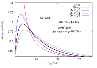
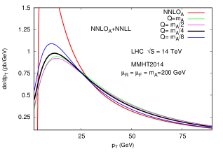
(a)	(b)

Figure 1: Resummation scale variation for (a) NLO+NLL and (b) NNLO_A+NNLL at 14 TeV

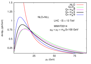
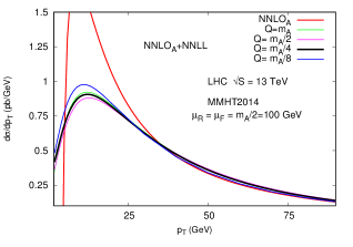
(a)	(b)

Figure 2: Resummation scale variation for (a) NLO+NLL and (b) NNLO_A+NNLL at 13 TeV

In Fig. 1 (14 TeV) and Fig. 2 (13 TeV) we study the effect of resummation over the fixed order result, where in each figure, the left panel shows the result for NLO and NLO+NLL; the right for NNLO_A and NNLO${}_{A}+$NNLL. For LHC 14TeV we set $\mu_{R}=\mu_{F}=m_{A}$; for LHC 13 TeV we keep $\mu_{R}=\mu_{F}=m_{A}/2$ and use MMHT2014 PDF sets for both the cases. We observe that the divergent behaviour of the distribution at fixed order is cured upon resummation. Precisely, at NLO the distribution diverges to positive infinity and at NNLO_A to negative infinity. Upon resummation a regular behaviour is displayed in both the cases.

Uncertainty due to $Q$:

in Fig. 1 and Fig. 2 we also show the sensitivity of the resummed results to the choice of resummation scale $Q$, where we have varied $Q$ from $m_{A}$ to $m_{A}/8$. For each diagram, in the left panel we see the results are quite sensitive to the choice, where by sensitivity we mean the range of variation of the maxima of distribution for different choices of Q. Not surprisingly, upon going to the next logarithmic accuracy (right panel) the sensitivity is significantly reduced around the peak region and the results at moderate values of $p_{T}$ are almost insensitive to the choice. It is reassuring that in the right panel at moderate and large values of $p_{T}$ the resummed curve is coincident with the fixed order curve, as desired. We note that the position of the peak is unchanged in going to the next order. For $Q=m_{A}$ and centre-of-mass energy 14 TeV we see that the peak value changes by 25% in going from NLO+NLL to NNLO_A+NNLL. Similarly for $Q=m_{A}/2$ and centre-of-mass energy 13 TeV, the peak value changes by 11% upon going from NLO+NLL to the next level of accuracy.

Uncertainty due to $\mu_{R}$ and $\mu_{F}$:

in Fig. 3(a) and Fig. 3(b)

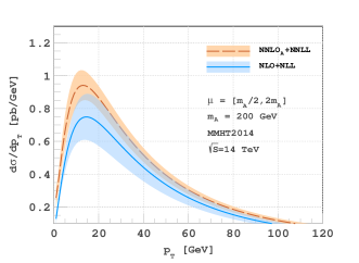
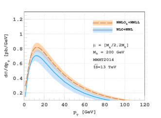
(a)	(b)

Figure 3: $\mu_{R}$ and $\mu_{F}$ variation at NLO+NLL and NNLO_A+NNLL for (a) 14 TeV and (b) 13 TeV

we show the sensitivity of our results to the variation of $\mu_{R}$ and $\mu_{F}$. The bands in this figure have been obtained by varying of $\mu_{R}$ and $\mu_{F}$ independently in the range $[m_{A}/2,2m_{A}]$, while excluding the regions where $\mu_{R}/\mu_{F}>2$ or $\mu_{R}/\mu_{F}<1/2$. More specifically, for 14 TeV centre-of-mass energy we see that at the peak, the variation is about $38\%$ for NLO+NLL which gets reduced to about $19\%$ upon going to the next level of accuracy. Similarly for 13 TeV centre-of-mass energy we see that at the peak the variation is about $22\%$ for NLO+NLL and about $15\%$ for NNLO_A+NNLL. We have also studied the individual variation of $\mu_{R}$ and $\mu_{F}$ for both the energies at the LHC in Fig. 4 and Fig. 5 respectively. In Fig. 4 we keep $\mu_{F}=m_{A}$ and vary $\mu_{R}$ in the range $[m_{A}/2,2m_{A}]$. For 14 TeV centre-of-mass energy we find that at the peak, the variation for NLO+NLL is about $32\%$, which gets reduced to about $17\%$ at NNLO_A+NNLL. Similarly for 13 TeV centre-of-mass energy we see that at the peak the variation is about $21\%$ for NLO+NLL and about $13\%$ for NNLO_A+NNLL. In Fig. 5 we set $\mu_{R}=m_{A}$ and vary $\mu_{F}$ in the same range as above. For 14 TeV centre-of-mass energy we find that at the peak, the variation for NLO+NLL is about $4\%$, which gets reduced to about $2\%$ at NNLO_A+NNLL. Similarly for 13 TeV centre-of-mass energy we see that at the peak the variation is about $4\%$ for NLO+NLL and about $0.5\%$ for NNLO_A+NNLL.

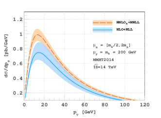
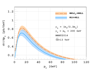
(a)	(b)

Figure 4: Variation of $\mu_{R}$ at NLO+NLL and NNLO_A+NNLL keeping $\mu_{F}$ fixed at $m_{A}$ for (a) 14 TeV and (b) 13 TeV

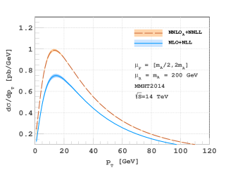
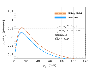
(a)	(b)

Figure 5: Variation of $\mu_{F}$ at NLO+NLL and NNLO_A+NNLL keeping $\mu_{R}$ fixed at $m_{A}$ for (a) 14 TeV and (b) 13 TeV

Combined uncertainty due to $Q,\mu_{R}$ and $\mu_{F}$:

in Fig. 6(a) and Fig. 6(b)

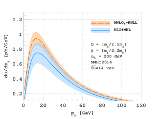
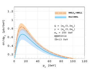
(a)	(b)

Figure 6: Q, $\mu_{R}$ and $\mu_{F}$ variation at NLO+NLL and NNLO_A+NNLL for (a) 14 TeV and (b) 13 TeV

we show the sensitivity of our results to the variation of Q, $\mu_{R}$ and $\mu_{F}$. The bands in this figure show independent variation of Q, $\mu_{R}$ and $\mu_{F}$ in the range $[m_{A}/2,2m_{A}]$ with constraints $\mu_{R}/\mu_{F}\in[1/2,\,2]$, $Q/\mu_{R}\in[1/2,\,2]$ and $Q/\mu_{F}\in[1/2,\,2]$. When we take into account all scale variations together we notice that both at 13 TeV and 14 TeV the variation at the peak is $38\%$ for NLO+NLL which gets reduced to $20\%$ upon going to the next level of accuracy. It is to be noted that this amount of decrement is almost same as the case discussed in Fig. 3(a).

Uncertainty due to parton density sets:

as there are several PDF groups in the literature, it is necessary to estimate the uncertainty resulting from the choice of PDFs within each set of a given PDF group. Using PDFs from different PDF groups namely MMHT2014 Harland-Lang:2014zoa , ABMP Alekhin:2017kpj , NNPDF3.1 Ball:2017nwa and PDF4LHC Butterworth:2015oua we have obtained the differential $p_{T}$ distributions along with the corresponding PDF uncertainty. In Fig. 7(a),

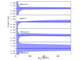
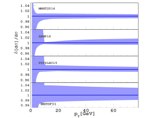
(a)	(b)

Figure 7: PDF variation at NNLO_A+NNLL for (a) 14 TeV and (b) 13 TeV using various sets. The y-axis represents the ratio of extremum variation over the central PDF set.

we have demonstrated the uncertainty bands for various PDF sets as a function of $p_{T}$ at energies of 14 TeV. In order to demonstrate the correlation of PDF uncertainty with the $p_{T}$ values we have tabulated in Table 1, the corresponding results for few benchmark values of $p_{T}$ along with percentage uncertainties. We have also performed the same exercise for 13 TeV centre of mass energy, as shown in Fig. 7(b). We have tabulated the results for few benchmark values of $p_{T}$ along with percentage uncertainties in Table 2.

$q_{T}$	MMHT	ABMP	NNPDF	PDF4LHC
7.0	$0.802^{+0.97\%}_{-1.75\%}$	$0.828^{+0.26\%}_{-0.78\%}$	$0.821^{+4.09\%}_{-3.00\%}$	$0.804^{+1.45\%}_{-0.91\%}$
13.0	$0.941^{+0.98\%}_{-1.07\%}$	$0.928^{+0.31\%}_{-0.49\%}$	$0.960^{+3.77\%}_{-2.60\%}$	$0.943^{+1.60\%}_{-0.80\%}$
19.0	$0.882^{+0.96\%}_{-1.05\%}$	$0.847^{+0.58\%}_{-0.55\%}$	$0.897^{+3.65\%}_{-2.53\%}$	$0.884^{+1.54\%}_{-0.67\%}$
25.0	$0.772^{+0.94\%}_{-1.01\%}$	$0.729^{+0.83\%}_{-0.60\%}$	$0.783^{+3.55\%}_{-2.45\%}$	$0.774^{+1.46\%}_{-0.56\%}$
31.0	$0.660^{+0.91\%}_{-0.96\%}$	$0.616^{+0.99\%}_{-0.63\%}$	$0.669^{+3.46\%}_{-2.38\%}$	$0.662^{+1.38\%}_{-0.61\%}$

Table 1: $q_{T}$ distributions at NNLO_A+NNLL using different PDF sets along with percentage uncertainties for $q_{T}=7.0,13.0,19.0,25.0,31.0$ for $\sqrt{s}=14$ TeV.

$q_{T}$	MMHT	ABMP	NNPDF	PDF4LHC
7.0	$0.762^{+0.99\%}_{-1.87\%}$	$0.783^{+18.52\%}_{-0.85\%}$	$0.780^{+22.04\%}_{-3.30\%}$	$0.761^{+23.32\%}_{-0.89\%}$
13.0	$0.880^{+1.01\%}_{-1.11\%}$	$0.864^{+0.34\%}_{-0.54\%}$	$0.898^{+3.93\%}_{-2.67\%}$	$0.882^{+1.56\%}_{-0.75\%}$
19.0	$0.820^{+0.98\%}_{-0.97\%}$	$0.783^{+0.57\%}_{-0.61\%}$	$0.834^{+3.84\%}_{-2.56\%}$	$0.822^{+1.51\%}_{-0.62\%}$
26.0	$0.698^{+0.94\%}_{-0.92\%}$	$0.654^{+0.85\%}_{-0.66\%}$	$0.707^{+3.70\%}_{-2.45\%}$	$0.700^{+1.43\%}_{-0.68\%}$
32.0	$0.596^{+0.91\%}_{-0.89\%}$	$0.552^{+0.99\%}_{-0.63\%}$	$0.602^{+3.60\%}_{-2.37\%}$	$0.597^{+1.35\%}_{-0.72\%}$

Table 2: $q_{T}$ distributions at NNLO_A+NNLL using different PDF sets along with percentage uncertainties for $q_{T}=7.0,13.0,19.0,26.0,32.0$ for $\sqrt{s}=13$ TeV.

Pseudo-scalar Higgs mass variation:

in Fig. 8(a) and Fig. 8(b)

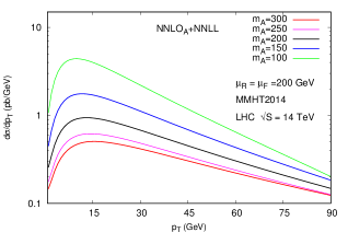
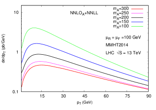
(a)	(b)

Figure 8: Pseudo-scalar Higgs mass variation at NNLO_A+NNLL for (a) 14 TeV and (b) 13 TeV

we show how the distribution behaves as the mass of the final state is changed. We have kept the renormalisation and factorisaiton scales fixed at $200$ GeV for 14 TeV, at 100 GeV for 13 TeV LHC energies and varied $m_{A}$ from $100$ to $300$ GeV. We see that the cross-section decreases with the increase in the mass of the final state.

4 Conclusion

In this study we obtained the resummed $p_{T}$ distribution for pseudo-scalar Higgs bosons at the LHC for both the centre-of-mass energy 14 TeV and 13 TeV at next-to-next-to-leading logarithmic accuracy by matching the resummed curve with approximated fixed order next-to-next-to-leading order result. We showed that we achieve a very significant reduction in sensitivity to the choices of resummation, renormalisation and factorisation scales that are artefact of perturbation theory. We also studied the uncertainty due to different choices of parton density sets. These results provide us with precise estimate for the distribution especially in the region around $15$ GeV where the cross-section is large and the fixed order results are completely unreliable due to the breakdown of fixed order perturbation series.

References

- (1) ATLAS collaboration, G. Aad et al., Observation of a new particle in the search for the Standard Model Higgs boson with the ATLAS detector at the LHC, Phys. Lett. B716 (2012) 1–29, [1207.7214].
- (2) CMS collaboration, S. Chatrchyan et al., Observation of a new boson at a mass of 125 GeV with the CMS experiment at the LHC, Phys. Lett. B716 (2012) 30–61, [1207.7235].
- (3) R. P. Kauffman and W. Schaffer, QCD corrections to production of Higgs pseudoscalars, Phys. Rev. D49 (1994) 551–554, [hep-ph/9305279].
- (4) A. Djouadi, M. Spira and P. M. Zerwas, Two photon decay widths of Higgs particles, Phys. Lett. B311 (1993) 255–260, [hep-ph/9305335].
- (5) M. Spira, A. Djouadi, D. Graudenz and P. M. Zerwas, Higgs boson production at the LHC, Nucl. Phys. B453 (1995) 17–82, [hep-ph/9504378].
- (6) M. Spira, A. Djouadi, D. Graudenz and P. M. Zerwas, SUSY Higgs production at proton colliders, Phys. Lett. B318 (1993) 347–353.
- (7) R. V. Harlander and W. B. Kilgore, Next-to-next-to-leading order Higgs production at hadron colliders, Phys. Rev. Lett. 88 (2002) 201801, [hep-ph/0201206].
- (8) R. V. Harlander and W. B. Kilgore, Production of a pseudoscalar Higgs boson at hadron colliders at next-to-next-to leading order, JHEP 10 (2002) 017, [hep-ph/0208096].
- (9) C. Anastasiou and K. Melnikov, Higgs boson production at hadron colliders in NNLO QCD, Nucl. Phys. B646 (2002) 220–256, [hep-ph/0207004].
- (10) C. Anastasiou and K. Melnikov, Pseudoscalar Higgs boson production at hadron colliders in NNLO QCD, Phys. Rev. D67 (2003) 037501, [hep-ph/0208115].
- (11) V. Ravindran, J. Smith and W. L. van Neerven, NNLO corrections to the total cross-section for Higgs boson production in hadron hadron collisions, Nucl. Phys. B665 (2003) 325–366, [hep-ph/0302135].
- (12) C. Anastasiou, C. Duhr, F. Dulat, F. Herzog and B. Mistlberger, Higgs Boson Gluon-Fusion Production in QCD at Three Loops, Phys. Rev. Lett. 114 (2015) 212001, [1503.06056].
- (13) R. V. Harlander and K. J. Ozeren, Top mass effects in Higgs production at next-to-next-to-leading order QCD: Virtual corrections, Phys. Lett. B679 (2009) 467–472, [0907.2997].
- (14) R. V. Harlander and K. J. Ozeren, Finite top mass effects for hadronic Higgs production at next-to-next-to-leading order, JHEP 11 (2009) 088, [0909.3420].
- (15) A. Pak, M. Rogal and M. Steinhauser, Finite top quark mass effects in NNLO Higgs boson production at LHC, JHEP 02 (2010) 025, [0911.4662].
- (16) C. Anastasiou, C. Duhr, F. Dulat, E. Furlan, T. Gehrmann, F. Herzog et al., Higgs boson gluon?fusion production at threshold in N3LO QCD, Phys. Lett. B737 (2014) 325–328, [1403.4616].
- (17) S. Moch and A. Vogt, Higher-order soft corrections to lepton pair and Higgs boson production, Phys. Lett. B631 (2005) 48–57, [hep-ph/0508265].
- (18) E. Laenen and L. Magnea, Threshold resummation for electroweak annihilation from DIS data, Phys. Lett. B632 (2006) 270–276, [hep-ph/0508284].
- (19) V. Ravindran, On Sudakov and soft resummations in QCD, Nucl. Phys. B746 (2006) 58–76, [hep-ph/0512249].
- (20) V. Ravindran, Higher-order threshold effects to inclusive processes in QCD, Nucl. Phys. B752 (2006) 173–196, [hep-ph/0603041].
- (21) A. Idilbi, X.-d. Ji, J.-P. Ma and F. Yuan, Threshold resummation for Higgs production in effective field theory, Phys. Rev. D73 (2006) 077501, [hep-ph/0509294].
- (22) M. C. Kumar, M. K. Mandal and V. Ravindran, Associated production of Higgs boson with vector boson at threshold N3LO in QCD, JHEP 03 (2015) 037, [1412.3357].
- (23) T. Ahmed, N. Rana and V. Ravindran, Higgs boson production through annihilation at threshold in N3LO QCD, JHEP 10 (2014) 139, [1408.0787].
- (24) T. Ahmed, M. C. Kumar, P. Mathews, N. Rana and V. Ravindran, Pseudo-scalar Higgs boson production at threshold N3 LO and N3 LL QCD, Eur. Phys. J. C76 (2016) 355, [1510.02235].
- (25) T. Ahmed, T. Gehrmann, P. Mathews, N. Rana and V. Ravindran, Pseudo-scalar Form Factors at Three Loops in QCD, JHEP 11 (2015) 169, [1510.01715].
- (26) S. Catani, D. de Florian, M. Grazzini and P. Nason, Soft gluon resummation for Higgs boson production at hadron colliders, JHEP 07 (2003) 028, [hep-ph/0306211].
- (27) S. Catani, L. Cieri, D. de Florian, G. Ferrera and M. Grazzini, Threshold resummation at N3LL accuracy and soft-virtual cross sections at N3LO, Nucl. Phys. B888 (2014) 75–91, [1405.4827].
- (28) M. Bonvini and S. Marzani, Resummed Higgs cross section at N3LL, JHEP 09 (2014) 007, [1405.3654].
- (29) M. Bonvini, S. Marzani, C. Muselli and L. Rottoli, On the Higgs cross section at N3LO+N3LL and its uncertainty, JHEP 08 (2016) 105, [1603.08000].
- (30) T. Ahmed, G. Das, M. C. Kumar, N. Rana and V. Ravindran, RG improved Higgs boson production to N3LO in QCD, 1505.07422.
- (31) T. Ahmed, M. Bonvini, M. C. Kumar, P. Mathews, N. Rana, V. Ravindran et al., Pseudo-scalar Higgs boson production at N3 LO +N3 LL ′, Eur. Phys. J. C76 (2016) 663, [1606.00837].
- (32) T. Schmidt and M. Spira, Higgs Boson Production via Gluon Fusion: Soft-Gluon Resummation including Mass Effects, Phys. Rev. D93 (2016) 014022, [1509.00195].
- (33) D. de Florian and J. Zurita, Soft-gluon resummation for pseudoscalar Higgs boson production at hadron colliders, Phys. Lett. B659 (2008) 813–820, [0711.1916].
- (34) P. Banerjee, G. Das, P. K. Dhani and V. Ravindran, Threshold resummation of the rapidity distribution for Higgs production at NNLO+NNLL, Phys. Rev. D97 (2018) 054024, [1708.05706].
- (35) P. Banerjee, G. Das, P. K. Dhani and V. Ravindran, Threshold resummation of the rapidity distribution for Drell-Yan production at NNLO+NNLL, 1805.01186.
- (36) G. F. Sterman, Summation of Large Corrections to Short Distance Hadronic Cross-Sections, Nucl. Phys. B281 (1987) 310–364.
- (37) S. Catani and L. Trentadue, Resummation of the QCD Perturbative Series for Hard Processes, Nucl. Phys. B327 (1989) 323–352.
- (38) S. Catani and L. Trentadue, Comment on QCD exponentiation at large x, Nucl. Phys. B353 (1991) 183–186.
- (39) E. Laenen and G. F. Sterman, Resummation for Drell-Yan differential distributions, in The Fermilab Meeting DPF 92. Proceedings, 7th Meeting of the American Physical Society, Division of Particles and Fields, Batavia, USA, November 10-14, 1992. Vol. 1, 2, pp. 987–989, 1992.
- (40) G. F. Sterman and W. Vogelsang, Threshold resummation and rapidity dependence, JHEP 02 (2001) 016, [hep-ph/0011289].
- (41) A. Mukherjee and W. Vogelsang, Threshold resummation for W-boson production at RHIC, Phys. Rev. D73 (2006) 074005, [hep-ph/0601162].
- (42) P. Bolzoni, Threshold resummation of Drell-Yan rapidity distributions, Phys. Lett. B643 (2006) 325–330, [hep-ph/0609073].
- (43) M. Bonvini, S. Forte and G. Ridolfi, Soft gluon resummation of Drell-Yan rapidity distributions: Theory and phenomenology, Nucl. Phys. B847 (2011) 93–159, [1009.5691].
- (44) M. A. Ebert, J. K. L. Michel and F. J. Tackmann, Resummation Improved Rapidity Spectrum for Gluon Fusion Higgs Production, JHEP 05 (2017) 088, [1702.00794].
- (45) T. Becher and M. Neubert, Threshold resummation in momentum space from effective field theory, Phys. Rev. Lett. 97 (2006) 082001, [hep-ph/0605050].
- (46) T. Becher, M. Neubert and G. Xu, Dynamical Threshold Enhancement and Resummation in Drell-Yan Production, JHEP 07 (2008) 030, [0710.0680].
- (47) Y. L. Dokshitzer, D. Diakonov and S. I. Troian, On the Transverse Momentum Distribution of Massive Lepton Pairs, Phys. Lett. 79B (1978) 269–272.
- (48) Y. L. Dokshitzer, D. Diakonov and S. I. Troian, Hard Processes in Quantum Chromodynamics, Phys. Rept. 58 (1980) 269–395.
- (49) G. Parisi and R. Petronzio, Small Transverse Momentum Distributions in Hard Processes, Nucl. Phys. B154 (1979) 427–440.
- (50) G. Curci, M. Greco and Y. Srivastava, QCD Jets From Coherent States, Nucl. Phys. B159 (1979) 451–468.
- (51) J. C. Collins and D. E. Soper, Back-To-Back Jets in QCD, Nucl. Phys. B193 (1981) 381.
- (52) J. Kodaira and L. Trentadue, Summing Soft Emission in QCD, Phys. Lett. 112B (1982) 66.
- (53) J. Kodaira and L. Trentadue, Single Logarithm Effects in electron-Positron Annihilation, Phys. Lett. 123B (1983) 335–338.
- (54) J. C. Collins, D. E. Soper and G. F. Sterman, Transverse Momentum Distribution in Drell-Yan Pair and W and Z Boson Production, Nucl. Phys. B250 (1985) 199–224.
- (55) S. Catani, E. D’Emilio and L. Trentadue, The Gluon Form-factor to Higher Orders: Gluon Gluon Annihilation at Small transverse, Phys. Lett. B211 (1988) 335–342.
- (56) D. de Florian and M. Grazzini, Next-to-next-to-leading logarithmic corrections at small transverse momentum in hadronic collisions, Phys. Rev. Lett. 85 (2000) 4678–4681, [hep-ph/0008152].
- (57) S. Catani, D. de Florian and M. Grazzini, Universality of nonleading logarithmic contributions in transverse momentum distributions, Nucl. Phys. B596 (2001) 299–312, [hep-ph/0008184].
- (58) H. X. Zhu, C. S. Li, H. T. Li, D. Y. Shao and L. L. Yang, Transverse-momentum resummation for top-quark pairs at hadron colliders, Phys. Rev. Lett. 110 (2013) 082001, [1208.5774].
- (59) H. T. Li, C. S. Li, D. Y. Shao, L. L. Yang and H. X. Zhu, Top quark pair production at small transverse momentum in hadronic collisions, Phys. Rev. D88 (2013) 074004, [1307.2464].
- (60) J. C. Collins and D. E. Soper, Back-To-Back Jets: Fourier Transform from B to K-Transverse, Nucl. Phys. B197 (1982) 446–476.
- (61) G. Altarelli, R. K. Ellis, M. Greco and G. Martinelli, Vector Boson Production at Colliders: A Theoretical Reappraisal, Nucl. Phys. B246 (1984) 12–44.
- (62) C. W. Bauer, S. Fleming and M. E. Luke, Summing Sudakov logarithms in B —¿ X(s gamma) in effective field theory, Phys. Rev. D63 (2000) 014006, [hep-ph/0005275].
- (63) C. W. Bauer, S. Fleming, D. Pirjol and I. W. Stewart, An Effective field theory for collinear and soft gluons: Heavy to light decays, Phys. Rev. D63 (2001) 114020, [hep-ph/0011336].
- (64) C. W. Bauer and I. W. Stewart, Invariant operators in collinear effective theory, Phys. Lett. B516 (2001) 134–142, [hep-ph/0107001].
- (65) C. W. Bauer, D. Pirjol and I. W. Stewart, Soft collinear factorization in effective field theory, Phys. Rev. D65 (2002) 054022, [hep-ph/0109045].
- (66) M. Beneke, A. P. Chapovsky, M. Diehl and T. Feldmann, Soft collinear effective theory and heavy to light currents beyond leading power, Nucl. Phys. B643 (2002) 431–476, [hep-ph/0206152].
- (67) G. Bozzi, S. Catani, D. de Florian and M. Grazzini, Higgs boson production at the LHC: Transverse-momentum resummation and rapidity dependence, Nucl. Phys. B791 (2008) 1–19, [0705.3887].
- (68) G. Bozzi, S. Catani, G. Ferrera, D. de Florian and M. Grazzini, Transverse-momentum resummation: A Perturbative study of Z production at the Tevatron, Nucl. Phys. B815 (2009) 174–197, [0812.2862].
- (69) S. Catani and M. Grazzini, QCD transverse-momentum resummation in gluon fusion processes, Nucl. Phys. B845 (2011) 297–323, [1011.3918].
- (70) S. Catani, M. Grazzini and A. Torre, Soft-gluon resummation for single-particle inclusive hadroproduction at high transverse momentum, Nucl. Phys. B874 (2013) 720–745, [1305.3870].
- (71) P. F. Monni, E. Re and P. Torrielli, Higgs Transverse-Momentum Resummation in Direct Space, Phys. Rev. Lett. 116 (2016) 242001, [1604.02191].
- (72) M. A. Ebert and F. J. Tackmann, Resummation of Transverse Momentum Distributions in Distribution Space, JHEP 02 (2017) 110, [1611.08610].
- (73) I. W. Stewart, F. J. Tackmann, J. R. Walsh and S. Zuberi, Jet resummation in Higgs production at , Phys. Rev. D89 (2014) 054001, [1307.1808].
- (74) M. Grazzini, S. Kallweit, D. Rathlev and M. Wiesemann, Transverse-momentum resummation for vector-boson pair production at NNLL+NNLO, JHEP 08 (2015) 154, [1507.02565].
- (75) G. Ferrera and J. Pires, Transverse-momentum resummation for Higgs boson pair production at the LHC with top-quark mass effects, JHEP 02 (2017) 139, [1609.01691].
- (76) A. Belyaev, P. M. Nadolsky and C. P. Yuan, Transverse momentum resummation for Higgs boson produced via b anti-b fusion at hadron colliders, JHEP 04 (2006) 004, [hep-ph/0509100].
- (77) R. V. Harlander, A. Tripathi and M. Wiesemann, Higgs production in bottom quark annihilation: Transverse momentum distribution at NNLONNLL, Phys. Rev. D90 (2014) 015017, [1403.7196].
- (78) W. Bizon, P. F. Monni, E. Re, L. Rottoli and P. Torrielli, Momentum-space resummation for transverse observables and the Higgs p⟂ at N3LL+NNLO, JHEP 02 (2018) 108, [1705.09127].
- (79) X. Chen, T. Gehrmann, E. W. N. Glover, A. Huss, Y. Li, D. Neill et al., Precise QCD Description of the Higgs Boson Transverse Momentum Spectrum, 1805.00736.
- (80) W. Bizo?, X. Chen, A. Gehrmann-De Ridder, T. Gehrmann, N. Glover, A. Huss et al., Fiducial distributions in Higgs and Drell-Yan production at N3LL+NNLO, 1805.05916.
- (81) J. Alwall, R. Frederix, S. Frixione, V. Hirschi, F. Maltoni, O. Mattelaer et al., The automated computation of tree-level and next-to-leading order differential cross sections, and their matching to parton shower simulations, JHEP 07 (2014) 079, [1405.0301].
- (82) S. Alioli, P. Nason, C. Oleari and E. Re, A general framework for implementing NLO calculations in shower Monte Carlo programs: the POWHEG BOX, JHEP 06 (2010) 043, [1002.2581].
- (83) M. Dasgupta, F. A. Dreyer, K. Hamilton, P. F. Monni and G. P. Salam, Logarithmic accuracy of parton showers: a fixed-order study, 1805.09327.
- (84) P. Banerjee, P. K. Dhani and V. Ravindran, Two loop QCD corrections for the process Pseudo-scalar Higgs partons, JHEP 10 (2017) 067, [1708.02387].
- (85) B. Field, Next-to-leading log resummation of scalar and pseudoscalar Higgs boson differential cross-sections at the CERN LHC and Tevatron, Phys. Rev. D70 (2004) 054008, [hep-ph/0405219].
- (86) G. Bozzi, S. Catani, D. de Florian and M. Grazzini, Transverse-momentum resummation and the spectrum of the Higgs boson at the LHC, Nucl. Phys. B737 (2006) 73–120, [hep-ph/0508068].
- (87) K. G. Chetyrkin, B. A. Kniehl, M. Steinhauser and W. A. Bardeen, Effective QCD interactions of CP odd Higgs bosons at three loops, Nucl. Phys. B535 (1998) 3–18, [hep-ph/9807241].
- (88) C. T. H. Davies, B. R. Webber and W. J. Stirling, Drell-Yan Cross-Sections at Small Transverse Momentum, Nucl. Phys. B256 (1985) 413.
- (89) D. de Florian and M. Grazzini, The Structure of large logarithmic corrections at small transverse momentum in hadronic collisions, Nucl. Phys. B616 (2001) 247–285, [hep-ph/0108273].
- (90) T. Becher and M. Neubert, Drell-Yan Production at Small , Transverse Parton Distributions and the Collinear Anomaly, Eur. Phys. J. C71 (2011) 1665, [1007.4005].
- (91) C. P. Yuan, Kinematics of the Higgs boson at hadron colliders: NLO QCD gluon resummation, Phys. Lett. B283 (1992) 395–402.
- (92) O. V. Tarasov, A. A. Vladimirov and A. Yu. Zharkov, The Gell-Mann-Low Function of QCD in the Three Loop Approximation, Phys. Lett. 93B (1980) 429–432.
- (93) S. Catani, L. Cieri, D. de Florian, G. Ferrera and M. Grazzini, Universality of transverse-momentum resummation and hard factors at the NNLO, Nucl. Phys. B881 (2014) 414–443, [1311.1654].
- (94) G. Bozzi, S. Catani, D. de Florian and M. Grazzini, The q(T) spectrum of the Higgs boson at the LHC in QCD perturbation theory, Phys. Lett. B564 (2003) 65–72, [hep-ph/0302104].
- (95) D. de Florian, G. Ferrera, M. Grazzini and D. Tommasini, Transverse-momentum resummation: Higgs boson production at the Tevatron and the LHC, JHEP 11 (2011) 064, [1109.2109].
- (96) L. A. Harland-Lang, A. D. Martin, P. Motylinski and R. S. Thorne, Parton distributions in the LHC era: MMHT 2014 PDFs, Eur. Phys. J. C75 (2015) 204, [1412.3989].
- (97) S. Alekhin, J. Blümlein, S. Moch and R. Placakyte, Parton distribution functions, , and heavy-quark masses for LHC Run II, Phys. Rev. D96 (2017) 014011, [1701.05838].
- (98) NNPDF collaboration, R. D. Ball et al., Parton distributions from high-precision collider data, Eur. Phys. J. C77 (2017) 663, [1706.00428].
- (99) J. Butterworth et al., PDF4LHC recommendations for LHC Run II, J. Phys. G43 (2016) 023001, [1510.03865].