Interaction-induced time-symmetry breaking in driven quantum oscillators

Abstract

We study parametrically driven quantum oscillators and show that, even for weak coupling between the oscillators, they can exhibit various many-body states with broken time-translation symmetry. In the quantum-coherent regime, the symmetry breaking occurs via a nonequilibrium quantum phase transition. For dissipative oscillators, the main effect of the weak coupling is to make the switching rate of an oscillator between its period-2 states dependent on the states of other oscillators. This allows mapping the oscillators onto a system of coupled spins. Away from the bifurcation parameter values where the period-2 states emerge, the stationary state corresponds to having a microscopic current in the spin system, in the presence of disorder. In the vicinity of the bifurcation point or for identical oscillators, the stationary state can be mapped on that of the Ising model with an effective temperature $\propto\hbar$, for low temperature. Closer to the bifurcation point the coupling can not be considered weak and the system maps onto coupled overdamped Brownian particles performing quantum diffusion in a potential landscape.

I Introduction

Time-symmetry breaking in periodically modulated quantum systems, often called a “time crystal” effect Wilczek (2012), has been attracting much attention recently. One of the most challenging problems in this rapidly developing area is the understanding of the interplay of interaction, disorder, and dissipation Khemani et al. (2016); Else et al. (2016); von Keyserlingk and Sondhi (2016); Yao et al. (2017); Zhang et al. (2017); Choi et al. (2017); Rovny et al. (2018); Berdanier et al. (2018). In particular, disorder helps preventing heating of the system by a periodic drive in the coherent regime Abanin et al. (2016); Bordia et al. (2017); Abanin et al. (2017). However, the dependence of the lifetime of the broken-symmetry state on the disorder strength is not known generally and is likely to be model-dependent. Disorder should not be necessary in the presence of dissipation. An example is the observation of an interaction-induced breaking of the time-translation symmetry in a dissipative classical cold-atom system Kim et al. (2006). A microscopic theory mapped the effect onto a phase transition in an all-to-all coupled Ising system, and the measured critical exponents were in agreement with this mapping Heo et al. (2010).

Closely related to the problem of time-symmetry breaking is computing with parametric oscillators Wang et al. (2013); McMahon et al. (2016); Inagaki et al. (2016); Goto (2016); Nigg et al. (2017); Puri et al. (2017); Goto et al. (2018). A weakly nonlinear classical dissipative oscillator displays period doubling when its eigenfrequency $\omega_{0}$ is modulated at a frequency $\omega_{F}$ close to $2\omega_{0}$ Landau and Lifshitz (2004). The emerging period-2 states have opposite phases, see Fig. 1. If the system is in one of these states, time-translation symmetry is broken, since the period of the motion is $4\pi/\omega_{F}\approx 2\pi/\omega_{0}$ instead of $2\pi/\omega_{F}$. These states can be associated with two states of a classical bit Woo and Landauer (1971), or two spin states. The spin analogy was studied in recent numerical work for up to four coupled quantum parametric oscillators and, for a number of parameter values, it was shown that the system can be mapped onto an “Ising machine” in the coherent Goto (2016) as well as the dissipative regime Nigg et al. (2017); Puri et al. (2017); Goto et al. (2018).

In this paper we study the possibility and the nature of time-symmetry breaking in a large system of coupled quantum parametric oscillators. Our formulation applies in the presence of weak disorder, but of primary interest to us are the broken-symmetry phases that emerge in the coherent and dissipative regimes and the associated phase transitions that occur even without disorder. The relevant physical systems are microwave modes in superconducting cavities that can be coupled into lattices with variable geometry Underwood et al. (2016); Kollár et al. (2018); Kounalakis et al. (2018), as well as coupled vibrational modes in networks of nanomechanical resonators Buks and Roukes (2002); Fon et al. (2017). An advantageous feature of these systems is the possibility to make them one- or two-dimensional, control the coupling strength, and implement various coupling geometries which, at least in the nanomechanical setting, are not limited to nearest-neighbor coupling. We assume the coupling of the modes in different resonators to be comparatively weak and the mode eigenfrequencies to form a narrow band centered at a characteristic eigenfrequency $\omega_{0}$. In the absence of a periodic drive, the spectrum of excitations is therefore also a narrow band centered near $\omega_{0}$.

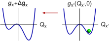
Figure 1: Left panel: Period doubling of a weakly nonlinear classical dissipative oscillator whose eigenfrequency $\omega_{0}$ is modulated at frequency $\omega_{F}\approx 2\omega_{0}$. Right two panels: The effective double-well Hamiltonian of a parametric oscillator as a function of its coordinate in the rotating frame. The right panel refers to an isolated oscillator, where the Hamiltonian $g_{\varkappa^{\prime}}(Q_{\varkappa^{\prime}},P_{\varkappa^{\prime}})$ is symmetric. The central panel shows how the Hamiltonian $g_{\varkappa}(Q_{\varkappa},0)$ is modified by an extra term $\Delta g_{\varkappa}$ due to the coupling to an oscillator $\varkappa^{\prime}$, which occupies a broken-symmetry state, as sketched in the right panel. The arrow indicates where the asymmetry is coming from.

The effect of the coupling is significantly more complicated for parametrically excited modes. To understand it, we note first that the quantum dynamics of an isolated mode can be mapped onto the dynamics of an auxiliary particle with a double-well quasienergy Hamiltonian Marthaler and Dykman (2006). The Hamiltonian is symmetric; the two minima correspond to the opposite phases of the period-2 oscillations, see the right panel in Fig. 1. The mode can tunnel between the minima, which leads to phase-flip transitions. However, if the relaxation rate largely exceeds the tunnel splitting, the interwell switching occurs via effectively “overbarrier” transitions. This happens even for $T=0$ due to quantum noise, which invariably accompanies relaxation Marthaler and Dykman (2006). One can associate the minima of the Hamiltonian of the $\varkappa$th mode with a spin $\sigma_{\varkappa}=\pm 1$. The switching rates $W_{\sigma_{\varkappa}}\equiv W_{\sigma_{\varkappa}\to-\sigma_{\varkappa}}$ between the minima are equal by symmetry.

If the modes are coupled and one of them is in a certain state (near one of the minima of the quasienergy Hamiltonian, see Fig. 1), the symmetry of the effective Hamiltonian for the mode coupled to it is broken. Then, for this mode, the switching rates between the minima become different. Depending on the sign of the coupling, the “deeper” well corresponds to the oscillators having the same (for the case of attractive coupling) or the opposite (for the case of repulsive coupling) phase.

It is important that the rates $W_{\sigma_{\varkappa}}$ are much smaller than the inverse $t_{r}^{-1}$ of the relaxation time. Therefore, when one of the modes is switching, the modes coupled to it are most likely localized in a certain minimum. As we show, the change of the switching rate $W_{\sigma_{\varkappa}}$ of mode $\varkappa$ due to its coupling to modes $\varkappa^{\prime}$ can be large even for weak coupling, with $\log W_{\sigma_{\varkappa}}$ being linear in the coupling. This allows one to map the problem onto the Ising model of coupled spins, for identical oscillators.

The well-known properties of the Ising model imply that, for not too weak attractive coupling, the most probable state of the many-mode two-dimensional system is the broken-symmetry state with all $\sigma_{\varkappa}$ equal, i.e., the phases of all oscillators being the same. In this state, the symmetry with respect to time translation by the drive period is broken. For the case of repulsive mode coupling, the system of coupled modes maps onto the antiferromagnetically coupled Ising model and can exhibit frustration, depending on the geometry of the lattice and the structure of the coupling.

Explicit analytical expressions for the coupling parameters of the Ising model can be obtained near the bifurcation point where the period-2 states of the individual modes emerge. As the parameters approach this point, the effective coupling strength increases. Ultimately, the system goes into the strong-coupling regime, and the mapping on the Ising model becomes inadequate. The modes strongly mix, and one can no longer think of an ensemble of individual modes having their own double-well quasienergy Hamiltonian.

For strong coupling, the appropriate picture is that of a multiple-well “quasienergy landscape”. This landscape has global symmetry with respect to time translation $t\to t+2\pi/\omega_{F}$, but each individual minimum does not have this symmetry. As a result, there are many metastable broken-symmetry states. Quantum noise leads to diffusion between these states, but the transitions between different minima involve many modes and become exponentially slow. The system effectively “freezes” in one of them, and time-translation symmetry is then broken.

In the quantum-coherent regime, a new phenomenon appears: instead of a bifurcation point for each individual oscillator, the coupled modes exhibit a nonequilibrium quantum phase transition (QPT). The control parameter is the distance to the critical value of the drive frequency $\omega_{F}=\omega_{\rm QPT}$, or to the critical value of the drive amplitude. We will consider the case where there is no disorder. The spectrum of excitations of the system can be naturally defined, if one starts from below the QPT, where the modes are not excited and all of them occupy the ground state. Here the spectrum is gapped, see Fig. 2. The simplest way to picture this situation is to think of the excitation spectrum of the coupled system in the absence of the drive, with the excitation frequency downshifted by $\omega_{F}/2$. The gap goes to zero at the phase transition point and the dispersion law of the long-wavelength excitations becomes linear. For attractive coupling between the modes, beyond the QPT the system has a state where all modes vibrate in phase and the excitation spectrum is again gapped. This state has broken time-translation symmetry, a direct analog of the ferromagnetic state of an Ising chain that goes through a QPT on varying the transverse magnetic field Lieb et al. (1961); Sachdev (1999).

Figure 2: Schematic view of the excitation spectrum $\omega(k)$ on going through the quantum phase transition. If the control parameter $\mu$ is below (left panel) or above (right panel) the critical value $\mu_{\rm QPT}$, the spectrum is gapped. For $\mu=\mu_{\rm QPT}$, the spectrum becomes linear for $k\to 0$.

The paper is organzied as follows: In Sec. II below we describe the Hamiltonian of the system. In Sec. III we show how the problem of weakly coupled parametric oscillators can be described in terms of the exponentially strong modification of the rate of interstate switching of an oscillator depending on the state of other oscillators. The description is based on the notion of the logarithmic susceptibility. It allows mapping the system onto an Ising system provided there is detailed balance. This is the case if the oscillators are identical. In Sec. IV we describe how to find the quantum logarithmic susceptibility for weak damping. Section V describes a theory of the coupled oscillators near the threshold of parametric excitation. It also describes a spin-glass type case where the system can have many metastable states with broken time-translation symmetry. Section VI describes a quantum time-symmetry breaking transition in a spatially-periodic system of coupled oscillators. Section VII contains concluding remarks.

II The model

We consider a system of coupled quantum oscillators (modes). They are weakly nonlinear and are parametrically modulated. The Hamiltonian of the system is

$$H=H_{0}+H_{F}+H_{c}\>,$$ (1)

where

$$H_{0}=\frac{1}{2}\sum_{\varkappa}(p_{\varkappa}^{2}+\omega_{\varkappa}^{2}q_{\varkappa}^{2})+\frac{1}{4}\gamma\sum_{\varkappa}q_{\varkappa}^{4}\>.$$ (2)

Here, $\varkappa=1,2,\ldots,N$ enumerates the oscillators, $q_{\varkappa}$ and $p_{\varkappa}$ are their coordinates and momenta, and $\omega_{\varkappa}$ are their eigenfrequencies; we assume that the values of $\omega_{\varkappa}$ are close to each other, $|\omega_{\varkappa}-\omega_{0}|\ll\omega_{0}$. The parameter $\gamma$ characterizes the lowest-order nonlinearity that is relevant for resonantly excited small-amplitude oscillations Landau and Lifshitz (2004). In what follows we assume $\gamma>0$; an extension to the case $\gamma<0$ is straightforward.

The Hamiltonian $H_{F}$ describes resonant parametric driving,

$$H_{F}=\frac{1}{2}\sum_{\varkappa}q_{\varkappa}^{2}F\cos\omega_{F}t,\quad\omega_{F}\approx 2\omega_{0}\>,$$ (3)

and $H_{c}$ is the Hamiltonian of the coupling between the modes,

$$H_{c}=-\frac{1}{2}\sum_{\varkappa\neq\varkappa^{\prime}}\varepsilon_{\varkappa\varkappa^{\prime}}q_{\varkappa}q_{\varkappa^{\prime}}\>,\quad|\varepsilon_{\varkappa\varkappa^{\prime}}|\ll\omega_{0}^{2}\>.$$ (4)

This interaction corresponds to bilinear mode coupling and occurs, e.g., in microwave cavity arrays and in systems of mechanical nanoresonators Kollár et al. (2018); Buks and Roukes (2002); Fon et al. (2017). The oscillator nonlinearity, the coupling, and the driving are assumed to be weak, $\gamma\langle q_{\varkappa}^{2}\rangle,|\varepsilon_{\varkappa\varkappa^{\prime}}|,|F|\ll\omega_{0}^{2}$. In this case the motion of the oscillators corresponds to vibrations at frequency $\approx\omega_{F}/2$ with amplitude and phase that slowly vary on the time scale $1/\omega_{F}$. This motion can be conveniently described in the rotating frame by introducing the ladder operators $a_{\varkappa},a^{\dagger}_{\varkappa}$ of the $\varkappa$th oscillator, applying a canonical transformation $U(t)=\exp[-i(\omega_{F}t/2)\sum_{\varkappa}a_{\varkappa}^{\dagger}a_{\varkappa}]$ and switching to the scaled coordinates $Q_{\varkappa}$ and momenta $P_{\varkappa}$ that slowly vary in time,

$$U^{\dagger}(t)[q_{\varkappa}+(2i/\omega_{F})p_{\varkappa}]U(t)=-iC(Q_{\varkappa}+iP_{\varkappa})e^{-i\omega_{F}t/2},$$

$$[P_{\varkappa},Q_{\varkappa^{\prime}}]=-i\lambda\delta_{\varkappa\varkappa^{\prime}},\qquad\lambda=3\hbar\gamma/\omega_{F}F.$$ (5)

Here, we set $C=(2F/3\gamma)^{1/2}=(2\hbar/\lambda\omega_{F})^{1/2}$; in Appendix A we use a different scaling to describe the quantum phase transition induced by the varying field amplitude. The parameter $\lambda$ is the dimensionless Planck constant in the rotating frame; we note that, in terms of the scaled variables $Q_{\varkappa},P_{\varkappa}$, the lowering operator is $a_{\varkappa}=(2\lambda)^{-1/2}(Q_{\varkappa}+iP_{\varkappa})$.

We assume that the scaled Planck constant is small, $\lambda\ll 1$. This means that the dynamics in the rotating frame is semiclassical and the states of parametrically excited period-2 oscillations of the individual mode overlap only weakly.

II.1 The rotating wave approximation

For weak nonlinearity and weak mode coupling, the resonant dynamics of the coupled modes can be conveniently described in the rotating wave approximation (RWA). In this approximation the canonically transformed Hamiltonian of the system becomes

$$U^{\dagger}HU-i\hbar U^{\dagger}\dot{U}\approx(3\gamma C^{4}/8){\mathbb{G}}\>,$$

$${\mathbb{G}}=\sum_{\varkappa}g_{\varkappa}(Q_{\varkappa},P_{\varkappa})+g_{c}\>.$$ (6)

Here, ${\mathbb{G}}$ is the scaled RWA Hamiltonian of the system. It is the sum of the scaled RWA Hamiltonians $g_{\varkappa}(Q_{\varkappa},P_{\varkappa})\equiv g_{\varkappa}(Q_{\varkappa},-i\lambda\partial_{Q_{\varkappa}})$ of the individual oscillators and the coupling term $g_{c}$. The individual Hamiltonians $g_{\varkappa}$ depend on a single parameter $\mu_{\varkappa}$ and can be expressed as Marthaler and Dykman (2006)

$$g_{\varkappa}(Q_{\varkappa},P_{\varkappa})=\frac{1}{4}(P_{\varkappa}^{2}+Q_{\varkappa}^{2}-\mu_{\varkappa})^{2}+\frac{1}{2}(P_{\varkappa}^{2}-Q_{\varkappa}^{2})-\frac{\mu_{\varkappa}^{2}}{4}\>,$$

$$\mu_{\varkappa}=2\delta\omega_{\varkappa}\omega_{F}/F,\qquad\delta\omega_{\varkappa}=\frac{1}{2}\omega_{F}-\omega_{\varkappa}\>.$$ (7)

The parameter $\mu_{\varkappa}$ is determined by the ratio of two small parameters, the detuning $\delta\omega_{\varkappa}$ of half the drive frequency from the mode eigenfrequency and the scaled drive amplitude $F/\omega_{F}$. For $\mu_{\varkappa}<-1$, $g_{\varkappa}(Q_{\varkappa},P_{\varkappa})$ has a single minimum at $Q_{\varkappa}=P_{\varkappa}=0$. This minimum corresponds to the equilibrium position of the oscillator in the laboratory frame. As $\mu_{\varkappa}$ increases beyond $-1$, the point $Q_{\varkappa}=P_{\varkappa}=0$ becomes first a saddle point, and then, for $\mu_{\varkappa}>1$, a local maximum of $g_{\varkappa}$. In addition, for $\mu_{\varkappa}>-1$, the function $g_{\varkappa}$ has two symmetrically located minima at $P_{\varkappa}=0,Q_{\varkappa}=\pm(\mu_{\varkappa}+1)^{1/2}$. They can be seen in the right panel of Fig. 1, which shows $g_{\varkappa}$ for $P_{\varkappa}=0$. Classically, in the presence of weak dissipation these minima become stable states. They correspond to two states of period-2 oscillations with opposite phases. We enumerate them by $\sigma_{\varkappa}=\pm 1$; for concreteness, we set $\sigma_{\varkappa}=1$ to correspond to the minimum of $g_{\varkappa}$ with $Q_{\varkappa}>0$.

The term $g_{c}$ in Eq. (II.1) describes the coupling Hamiltonian in the rotating frame,

$$g_{c}=-\frac{1}{2}\sum_{\varkappa\neq\varkappa^{\prime}}V_{\varkappa\varkappa^{\prime}}(Q_{\varkappa}Q_{\varkappa^{\prime}}+P_{\varkappa}P_{\varkappa^{\prime}})\>,$$

$$V_{\varkappa\varkappa^{\prime}}=2\varepsilon_{\varkappa\varkappa^{\prime}}/F\>.$$ (8)

We note that the coupling in the coordinate channel in the lab frame described by Eq. (4) becomes symmetric with respect to the coordinates and momenta in the rotating frame, in the RWA.

The effect of the coupling on the mode dynamics depends on the relation between $|V_{\varkappa\varkappa^{\prime}}|$ and the depth of the wells of the functions $g_{\varkappa}$, see Fig. 1. If $|V_{\varkappa\varkappa^{\prime}}|\ll 1$, the overall many-mode Hamiltonian (II.1) is a set of double-well functions $g_{\varkappa}$ slightly distorted by the coupling (unless $\mu_{\varkappa}-1$ is also small, see below). If, on the other hand, the coupling is comparatively strong, the overall structure of the Hamiltonian changes. We will not consider this case in the present paper.

II.1.1 Symmetry arguments

The RWA Hamiltonian ${\mathbb{G}}$ has inversion symmetry, both in the coordinates, $\{Q_{\varkappa}\to-Q_{\varkappa}\}$, and in the momenta, $\{P_{\varkappa}\to-P_{\varkappa}\}$. This symmetry is a consequence of the symmetry of the Hamiltonian $H$ with respect to time translation by the driving period $t\to t+2\pi/\omega_{F}$. From Eq. (II), such a translation corresponds to changing the signs of $\{Q_{\varkappa},P_{\varkappa}\}$. Indeed, as a result of the time translation, the unitary operator $U(t)$ in Eq. (II) becomes $U(t+2\pi/\omega_{F})=U(t)N_{2}$, where $N_{2}=\exp(-i\pi\sum_{\varkappa}a_{\varkappa}^{\dagger}a_{\varkappa})$. The time-translation operator $N_{2}$ flips the sign of the mode coordinates and momenta, $N_{2}^{\dagger}q_{\varkappa}N_{2}=-q_{\varkappa}$ and similarly for $p_{\varkappa}$. In addition, $N_{2}$ commutes with ${\mathbb{G}}$. Therefore, as in the case of a single oscillator Guo et al. (2013a); Zhang et al. (2017), the eigenfunctions of ${\mathbb{G}}$ are the Floquet eigenfunctions of the original time-periodic Hamiltonian $H$, and the eigenvalues of ${\mathbb{G}}$ are the RWA-quasienergies of the system scaled by the factor $3\gamma C^{4}/8$.

The individual RWA Hamiltonians $g_{\varkappa}$ also have inversion symmetry, cf. Fig. 1. Therefore, generally, the intrawell states of $g_{\varkappa}$ are tunnel-split into symmetric and antisymmetric states. For a small dimensionless Planck constant $\lambda$, this splitting is exponentially small deep inside the wells and may be equal to zero for certain $\mu_{\varkappa}$ Marthaler and Dykman (2007); *Zhang2017a.

II.2 Quantum kinetic equation

We now discuss the dissipative dynamics of the system of parametric oscillators. To this end, we will assume that each oscillator is coupled to its own thermal reservoir and that all reservoirs have the same temperature. We will use the simplest model where the interaction with the reservoirs is linear in $q_{\varkappa},p_{\varkappa}$. If the densities of states of the reservoirs weighted with the coupling to the environment are sufficiently smooth near $\omega_{0}$, the dynamics of the nonlinear oscillators in “slow time”

$$\tau\equiv tF/2\omega_{F}$$ (9)

is Markovian. A derivation is a straightforward extension of the derivation for a single nonlinear oscillator Dykman and Krivoglaz (1984) to the case of coupled oscillators; the frequency renormalization is incorporated into $\omega_{\varkappa}$. For simplicity, we will assume that the decay rates of all the oscillators are the same: different decay rates constitute a dissipative type of disorder and will not be discussed in this paper. With these assumptions, the master equation for the multi-oscillator density matrix $\rho$ reads

$$\dot{\rho}\equiv\frac{d\rho}{d\tau}=\frac{i}{\lambda}\left[\rho,{\mathbb{G}}\right]+\kappa\sum_{\varkappa}{\cal D}[a_{\varkappa}]\rho\>,$$

$${\cal D}[a]\rho=-\left(\bar{n}+1\right)\left(a^{\dagger}a\rho-2a\rho a^{\dagger}+\rho a^{\dagger}a\right)$$

$$-\bar{n}\left(aa^{\dagger}\rho-2a^{\dagger}\rho a+\rho aa^{\dagger}\right)\>.$$ (10)

Here, $\kappa$ is the dimensionless oscillator decay rate and $\bar{n}=[\exp(\hbar\omega_{F}/2k_{B}T)-1]^{-1}$ is the oscillator Planck number.

Alternatively, and this will be used below, one can write down the quantum Langevin equations

$$\dot{Q}_{\varkappa}=-\kappa Q_{\varkappa}+\partial_{P_{\varkappa}}{\mathbb{G}}+f_{Q_{\varkappa}}(\tau)\>,$$

$$\dot{P}_{\varkappa}=-\kappa P_{\varkappa}-\partial_{Q_{\varkappa}}{\mathbb{G}}+f_{P_{\varkappa}}(\tau)\>.$$ (11)

Here, $f_{Q_{\varkappa}}(\tau)$ and $f_{P_{\varkappa}}(\tau)$ are $\delta$-correlated operators,

$$\langle f_{Q_{\varkappa}}(\tau)f_{Q_{\varkappa^{\prime}}}(\tau^{\prime})\rangle=\langle f_{P_{\varkappa}}(\tau)f_{P_{\varkappa^{\prime}}}(\tau^{\prime})\rangle$$

$$=2D\delta(\tau-\tau^{\prime})\delta_{\varkappa\varkappa^{\prime}},\qquad D=\frac{1}{2}\lambda\kappa(2\bar{n}+1),$$ (12)

and $\langle[f_{Q_{\varkappa}}(\tau),f_{P_{\varkappa^{\prime}}}(\tau^{\prime})]\rangle=2i\lambda\kappa\delta(\tau-\tau^{\prime})\delta_{\varkappa\varkappa^{\prime}}$. For small $\lambda$ the noise intensity $D$ is small. Equation (II.2) is the Heisenberg version of the master equation (II.2). The partial derivatives of ${\mathbb{G}}$ in Eq. (II.2) should be interpreted as symmetrized expressions, for example, $\partial_{P}(P^{2}+Q^{2})^{2}=2P(P^{2}+Q^{2})+2(P^{2}+Q^{2})P$.

III Time-symmetry breaking for weakly coupled modes

In this section we show that even weak mode coupling can lead to a collective breaking of the time-translation symmetry if the quantum noise is sufficiently weak. The underlying mechanism is the coupling-induced change of the rate of switching between the period-2 states of the oscillators.

The dissipative dynamics of an isolated parametric oscillator $\varkappa$ is characterized by the dimensionless relaxation rate $\kappa$ and by the dimensionless rate of switching $W_{\sigma_{\varkappa}}\equiv W_{\sigma_{\varkappa}\to-\sigma_{\varkappa}}$ between the wells $\sigma_{\varkappa}$ and $-\sigma_{\varkappa}$ of the RWA Hamiltonian $g_{\varkappa}$. The switching rates are exponentially smaller than the relaxation rate, i.e., $W_{\sigma_{\varkappa}}\ll\kappa$. The oscillator approaches one of the minima of $g_{\varkappa}$ on a time scale $\sim\kappa^{-1}$. It performs quantum fluctuations about this minimum for a time much longer than $\kappa^{-1}$, until ultimately it switches to the other minimum. We note that the notation $W_{\sigma_{\varkappa}}$ is a shortcut: it refers to the rate $W_{\varkappa}(\sigma_{\varkappa})$ for the $\varkappa$th oscillator to switch from the well $\sigma_{\varkappa}$ to $-\sigma_{\varkappa}$.

If $\kappa$ largely exceeds the exponentially small tunnel splitting of the intrawell states, the interwell switching occurs via “overbarrier” transitions Marthaler and Dykman (2006). Such transitions result from quantum diffusion over the intrawell quasienergy states, which brings the system from the bottom of the initially occupied well of $g_{\varkappa}$ to the top of the barrier. This process is reminiscent of the familiar thermally activated overbarrier transitions in classical systems Kramers (1940), except that, for low temperatures, it is induced by quantum fluctuations and is called quantum activation. The physical cause of the diffusion over quasienergy states is that quantum relaxation is invariably associated with noise. Relaxation results from transitions between the states of the oscillator with emission of excitations of the thermal reservoir, but these transitions happen at random, and therefore they bring in noise. The presence of this quantum noise is reflected in the noise terms in Eq. (II.2).

For an isolated oscillator $\varkappa$, the rate of switching due to quantum activation has the form

$$W_{\sigma_{\varkappa}}^{(0)}=\mathrm{const}\times\exp(-R_{\sigma_{\varkappa}}^{(0)}/\lambda).$$

The parameter $R_{\sigma_{\varkappa}}^{(0)}$ is the quantum activation energy of switching from state $\sigma_{\varkappa}$; note that the quantum noise intensity $\lambda$ plays here a role analogous to temperature in the expression for the rate of thermally activated switching. By symmetry, $R_{\sigma_{\varkappa}}^{(0)}$ is the same for the both states $\sigma_{\varkappa}=\pm 1$. Expressions for $R_{\sigma_{\varkappa}}^{(0)}$ have been found in several important limiting cases Marthaler and Dykman (2006); Dykman (2007).

III.1 Symmetry lifting by an extra field at frequency $\omega_{F}/2$

Before analyzing the effect of the coupling of the modes, we consider a simpler related problem, viz., the effect of a weak additional field at frequency $\omega_{F}/2$ on the switching rate. Such a field is described by the term $-F^{\prime}\sum_{\varkappa}q_{\varkappa}\cos(\varphi_{\varkappa}+\omega_{F}t/2)$ in the Hamiltonian. It breaks the time-translation symmetry $t\to t+2\pi/\omega_{F}$. In the rotating frame, the effect of the field $\propto F^{\prime}$ on the mode dynamics is described by the term

$$\Delta g_{\varkappa}(Q_{\varkappa},P_{\varkappa})=-f^{\prime}(Q_{\varkappa}\sin\varphi_{\varkappa}+P_{\varkappa}\cos\varphi_{\varkappa})$$ (13)

that has to be added to the RWA Hamiltonian $g_{\varkappa}$, Eq. (II.1), with $f^{\prime}=8F^{\prime}/3\gamma C^{3}$.

If the rescaled field $f^{\prime}$ is small, the term $\Delta g_{\varkappa}$ is small compared to the depth of the wells of $g_{\varkappa}$. However, it can lead to a significant change of the switching rates and, most importantly, make the switching rates $\sigma_{\varkappa}\rightarrow-\sigma_{\varkappa}$ different for $\sigma_{\varkappa}=1$ and $\sigma_{\varkappa}=-1$. In the stationary state, this will lead to a difference of the well populations. In the classical regime, where the interstate switching is thermally activated, the change was discussed previously Ryvkine and Dykman (2006). We will show in the following sections that, in the quantum regime, too, in several cases of interest the major effect of the drive is to change the quantum activation energy $R_{\sigma_{\varkappa}}$ compared to its value $R_{\sigma_{\varkappa}}^{(0)}$ in the absence of the drive (similar to the case of the switching rate, the notation $R_{\sigma_{\varkappa}}$ is used for the value of $R$ for the oscillator $\varkappa$ in the state $\sigma_{\varkappa}$). This leads to a corresponding change of the switching rate $W_{\sigma_{\varkappa}}$,

$$W_{\sigma_{\varkappa}}\propto\exp[-R_{\sigma_{\varkappa}}/\lambda]\>,\qquad R_{\sigma_{\varkappa}}=R_{\sigma_{\varkappa}}^{(0)}+\Delta R_{\sigma_{\varkappa}}\>,$$

$$\Delta R_{\sigma_{\varkappa}}=f^{\prime}\sigma_{\varkappa}(\chi_{Q\varkappa}\sin\varphi_{\varkappa}+\chi_{P\varkappa}\cos\varphi_{\varkappa})\>.$$ (14)

In analogy to the classical case, we introduced the logarithmic susceptibilities $\chi_{Q\varkappa}$ and $\chi_{P\varkappa}$ for the variables $Q_{\varkappa}$ and $P_{\varkappa}$ of the mode $\varkappa$. Note that to simplify the further analysis we use a notation that differs from the one used in Ref. Ryvkine and Dykman, 2006. To be specific, these susceptibilities will be calculated for the well $\sigma_{\varkappa}=1$. They give the change of the logarithm of the switching rate $W_{\sigma_{\varkappa}}$ linear in the drive $f^{\prime}$. The change of the rate can be large even if $|\Delta R_{\sigma_{\varkappa}}|\ll R_{\sigma_{\varkappa}}^{(0)}$ provided $|\Delta R_{\sigma_{\varkappa}}|\gg\lambda$. By symmetry, the sign of the change is opposite for the two different wells, and therefore $\Delta R_{\sigma_{\varkappa}}\propto\sigma_{\varkappa}$.

In the previous discussion we tacitly implied that the relaxation-induced broadening $\kappa\lambda$ of the eigenvalues of $g_{\varkappa}$, i.e., of the scaled quasienergy levels, is small compared to the level spacing. In this case, as we indicated, for isolated oscillators these are the intrawell states close to the bottom of the wells of $g_{\varkappa}$ that are primarily occupied. In the Wigner representation, the probability distribution $\rho_{\varkappa}(Q_{\varkappa},P_{\varkappa})$ of an isolated oscillator has peaks, which are centered close to the minima of $g_{\varkappa}(Q_{\varkappa},P_{\varkappa})$ and have a width $\sim\lambda^{1/2}$ Marthaler and Dykman (2006); Dykman (2007). However, if the level broadening is not small, the Wigner distribution $\rho_{\varkappa}$ can still be double-peaked. In the absence of a drive $F^{\prime}$ it is symmetric. The peaks are located at $(\sigma_{\varkappa}Q_{\varkappa}^{(0)},\sigma_{\varkappa}P_{\varkappa}^{(0)})$, with $\sigma_{\varkappa}=\pm 1$, and

$$Q_{\varkappa}^{(0)}=(\mu_{\varkappa}-\mu_{B})^{1/2}\cos\Phi_{\varkappa}\>,\quad\mu_{B}=-(1-\kappa^{2})^{1/2}\>,$$

$$P_{\varkappa}^{(0)}=(\mu_{\varkappa}-\mu_{B})^{1/2}\sin\Phi_{\varkappa}\>,\quad\Phi_{\varkappa}=\arctan\frac{\kappa}{1-\mu_{B}}\>.$$ (15)

The coordinates $Q_{\varkappa}^{(0)}$, $P_{\varkappa}^{(0)}$ are given by the stable stationary solution of the Langevin equation (II.2) disregarding the coupling between the modes and the quantum noise. The coefficient $\mu_{B}$ is the value of $\mu_{\varkappa}$ at the bifurcation where the zero-amplitude state $Q_{\varkappa}=P_{\varkappa}=0$ becomes dynamically unstable and the two stable period-2 states emerge. In the model we use here, where the decay rate in the scaled time is the same for all modes, $\mu_{B}$ is also the same for all modes.

III.2 Switching rates for coupled modes

The separation of the time scales of relaxation and interwell switching allows one to use the logarithmic susceptibilities to describe the effect of a weak interaction between the oscillators. In the absence of interaction, as seen from the master equation (II.2), on a time scale long compared to $\kappa^{-1}$, the dynamics of the modes can be described as rare uncorrelated switching events between the wells. Most of the time each oscillator spends in close vicinity of $\pm(Q_{\varkappa}^{(0)},P_{\varkappa}^{(0)})$. We emphasize that, in each of these states, the time-translation symmetry is broken.

The major effect of a weak interaction is that, if one oscillator is in a given state $\sigma=\pm 1$, it lifts the time-translation symmetry for the oscillators it is coupled to. In fact, it acts exactly like a driving force $\propto F^{\prime}$, as it also oscillates at frequency $\omega_{F}/2$. Put differently, for any given oscillator $\varkappa$, the oscillators $\varkappa^{\prime}$ with $\varkappa^{\prime}\neq\varkappa$ act as a drive at frequency $\omega_{F}/2$. The phase of this drive is determined by the states $\sigma_{\varkappa^{\prime}}$ of these oscillators. By comparing the expressions for the change of $g_{\varkappa}$ due to an external drive (13) with the expression (II.1) for the coupling term $g_{c}$, we see that the switching rates between the states of the considered oscillator $\varkappa$ have the form

$$W_{\sigma_{\varkappa}}=W_{\sigma_{\varkappa}}^{(0)}\exp\left[-\sigma_{\varkappa}\sum_{\varkappa^{\prime}}{\vphantom{\sum}}^{\!\!\prime}J_{\varkappa\varkappa^{\prime}}\sigma_{\varkappa^{\prime}}/\lambda{}\right]$$

$$J_{\varkappa\varkappa^{\prime}}=V_{\varkappa\varkappa^{\prime}}[\chi_{Q\varkappa}Q_{\varkappa^{\prime}}^{(0)}+\chi_{P\varkappa}P_{\varkappa^{\prime}}^{(0)}].$$ (16)

Here we have approximated the dynamical variables $Q_{\varkappa^{\prime}},P_{\varkappa^{\prime}}$ of the oscillators with $\varkappa^{\prime}\neq\varkappa$ by their most probable values $\sigma_{\varkappa^{\prime}}Q_{\varkappa^{\prime}}^{(0)},\sigma_{\varkappa^{\prime}}P_{\varkappa^{\prime}}^{(0)}$.

Equation (III.2) maps the problem of the coupled parametric oscillators onto a problem of coupled Ising spins. The effect of the spin coupling is to modify the rates of switching between the states of individual spins. If the oscillators slightly differ in frequency or one of the other parameters, the spin-coupling parameters are asymmetric, $J_{\varkappa\varkappa^{\prime}}\neq J_{\varkappa^{\prime}\varkappa}$. This is because the equilibrium positions of different oscillators in the rotating frame $(Q_{\varkappa},P_{\varkappa})$ are different and so are also the logarithmic susceptibilities.

III.3 The stationary distribution. Mapping onto the Ising model

We will now look at the evolution of the distribution $w(\sigma_{1},\sigma_{2},\ldots)$ of the states $\{\sigma_{\varkappa}\}$ of the system of effective spins. The distribution changes due to switching of the spins, that is, of the individual oscillators, with the rates from Eq. (III.2). Given that the switching events are independent, the function $w$ evolves according to the balance equation

$$\dot{w}= -\sum_{\varkappa}W_{\sigma_{\varkappa}}w(\sigma_{1},\ldots,\sigma_{\varkappa},\ldots)$$

$$+\sum_{\varkappa}W_{-\sigma_{\varkappa}}w(\sigma_{1},\ldots,-\sigma_{\varkappa},\ldots)\>.$$ (17)

Importantly, if the oscillators are different, implying $J_{\varkappa\varkappa^{\prime}}\neq J_{\varkappa^{\prime}\varkappa}$, the system lacks detailed balance. Indeed, consider the probability of a pair of switching events that bring the system from the state with given $(\sigma_{\varkappa},\sigma_{\varkappa^{\prime}})$ to $(-\sigma_{\varkappa},-\sigma_{\varkappa^{\prime}})$. It is easy to see that this probability then depends on which of the spins, $\varkappa$ or $\varkappa^{\prime}$, switches first for $J_{\varkappa\varkappa^{\prime}}\neq J_{\varkappa^{\prime}\varkappa}$. The violation of detailed balance is a generic feature of systems far from thermal equilibrium, and the system of driven oscillators considered here is in this category.

The dynamics of the system greatly simplifies in the case of identical oscillators or in the vicinity of the bifurcation point, see Secs. IV.1 and V, so that $J_{\varkappa\varkappa^{\prime}}=J_{\varkappa^{\prime}\varkappa}$. In this case the stationary solution of Eq. (III.3) is

$$w_{\rm st}=Z^{-1}\exp\left[-H(\{\sigma_{\varkappa}\})/\lambda\right]$$

$$H(\{\sigma_{\varkappa}\})=-\frac{1}{2}\sum_{\varkappa\neq\varkappa^{\prime}}J_{\varkappa\varkappa^{\prime}}\sigma_{\varkappa}\sigma_{\varkappa^{\prime}}\>.$$ (18)

This exactly corresponds to the statistical distribution of an Ising system at effective quantum temperature $\lambda$; the normalization constant $Z$ plays the role of the partition function. If the coupling constants of the oscillators $\varepsilon_{\varkappa\varkappa^{\prime}}\propto V_{\varkappa\varkappa^{\prime}}\propto J_{\varkappa\varkappa^{\prime}}$ are positive, the coupling is “ferromagnetic”: in the most probable state the values of $\sigma_{\varkappa}$ are the same for all oscillators, that is, the oscillators vibrate in phase. This is intuitively clear: if the oscillators attract each other, they will try to synchronize into a state where they all vibrate in phase. Whether the system reaches this fully ordered state is determined by the standard results for the ferromagnetic Ising model.

In the opposite case where $\varepsilon_{\varkappa\varkappa^{\prime}}$ are negative, Eq. (III.3) maps the system of parametric oscillators onto an antiferromagnetic Ising system. We emphasize that in the system of oscillators that are currently studied, both the strength of the coupling, and often its sign, can be independently controlled.

IV Quantum logarithmic susceptibility

To find the coupling parameters $J_{\varkappa\varkappa^{\prime}}$ one has first to calculate the logarithmic susceptibility of an isolated oscillator. A general approach to such a calculation is based on solving the variational problem for the exponent of the switching rate $R_{\sigma_{\varkappa}}$, which can be formulated using the master equation (II.2). We will use simpler approaches, which apply in the limiting cases. We will start with the case of weak damping, where the broadening of the quasienergy levels is small compared to the level spacing.

IV.1 Weak-damping limit

In the weak-damping limit, we write the master equation (II.2) for the isolated oscillator $\varkappa$ as a balance equation for the populations $\rho_{m_{\varkappa}}$ of the eigenstates $|m_{\varkappa}\rangle$ of the RWA Hamiltonian

$$G{}_{\varkappa}=g_{\varkappa}+\Delta g_{\varkappa}\>.$$ (19)

The operator $G_{\varkappa}$ describes an isolated parametric oscillator $\varkappa$ driven additionally by a weak field at half the frequency of the parametric drive. The term $\Delta g_{\varkappa}$ is given by Eq. (13); it is proportional to the weak field amplitude $F^{\prime}$.

For small $\lambda$ and $F^{\prime}$, the function $G{}_{\varkappa}(Q_{\varkappa},P_{\varkappa})$ has two slightly asymmetric wells (enumerated by $\sigma_{\varkappa}=\pm 1$), cf. Fig. 1. There are many eigenstates inside each of the wells for $\lambda\ll 1$. We consider the states $|m_{\varkappa}\rangle$ inside one of the wells and number them so that $m_{\varkappa}=0$ corresponds to the lowest state. Coupling to a thermal reservoir leads to transitions $|m_{\varkappa}+k_{\varkappa}\rangle\to|m_{\varkappa}\rangle$. From Eq. (II.2), the rates $\Lambda_{m_{\varkappa}+k_{\varkappa}\,m_{\varkappa}}$ of such intrawell transitions are given by the squared matrix elements of the operators $a_{\varkappa},a^{\dagger}_{\varkappa}$ on the corresponding wave functions,

$$\Lambda_{m_{\varkappa}+k_{\varkappa}\,m_{\varkappa}} =2\kappa(\bar{n}+1)\left|\langle m_{\varkappa}|a_{\varkappa}|m_{\varkappa}+k_{\varkappa}\rangle\right|^{2}$$

$$+2\kappa\bar{n}\left|\langle m_{\varkappa}+k_{\varkappa}|a_{\varkappa}|m_{\varkappa}\rangle\right|^{2}.$$ (20)

Generally, the rates of transitions with $k_{\varkappa}>0$ are higher than with $k_{\varkappa}<0$, i.e., the system is more likely to move to eigenstates with lower $G_{\varkappa}$. This corresponds to the minima of $G_{\varkappa}(Q_{\varkappa},P_{\varkappa})$ being stable states of the oscillator in the classical limit.

However, even for zero temperature, in contrast to equilibrium systems, transitions away from the minima of $G_{\varkappa}$, i.e., with $k_{\varkappa}<0$, have nonzero rates. They lead to the probability for an oscillator, starting from deep inside of a well, to reach the intrawell states near the top of the barrier of $G_{\varkappa}$. From there, the oscillator will end up in each of the two wells with probability $\sim 1/2$. The exponent of the switching rate $W_{\sigma_{\varkappa}}$ is thus determined by the population of the intrawell states $|m_{\varkappa}\rangle$ of the $\sigma_{\varkappa}$-well near the top of the barrier. The logarithmic susceptibility describes the linear dependence of the exponent of this population on the field $F^{\prime}$.

It is convenient to seek the state populations $\rho_{m_{\varkappa}}$ in the form $\rho_{m_{\varkappa}}=\exp[-R\bigl{(}G{}(m_{\varkappa})\bigr{)}/\lambda]$, where $G{}(m_{\varkappa})$ is the eigenvalue of $G{}_{\varkappa}$ in the state $|m_{\varkappa}\rangle$. This form of $\rho_{m_{\varkappa}}$ is reminiscent of a Boltzmann distribution, with $\lambda$ playing the role of the temperature and $R(G{})$ playing the role of the energy. In the considered nonequilibrium case, $R$ is not a linear function of $G{}$. The populations $\rho_{m_{\varkappa}}$ strongly vary with the level number $m_{\varkappa}$. However, generally, the function $R(G{})$ is smooth even for small $\lambda$.

The equation for $R(G{})$ can be obtained from the master equation in the eikonal (WKB) approximation. It is seen from Eq. (IV.1) that the intrawell transition rates $\Lambda_{m_{\varkappa}+k_{\varkappa}\,m_{\varkappa}}$ fall off exponentially fast with $|k_{\varkappa}|$. One can then expand $R\bigl{(}G{}(m_{\varkappa}+k_{\varkappa})\bigr{)}\approx R\bigl{(}G{}(m_{\varkappa})\bigr{)}+\lambda k_{\varkappa}[\omega(G{})dR/dG{}]_{m_{\varkappa}}$, which is essentially the eikonal approximation. Here, $\omega(G{})$ is the frequency of classical vibrations with a given $G{}$; we used that $\omega(G{}_{m_{\varkappa}})=[G{}(m_{\varkappa}+1)-G{}(m_{\varkappa})]/\lambda+o(\lambda)$; $[\cdot]_{m_{\varkappa}}$ indicates that the function of $G{}$ is evaluated for $G{}=G{}(m_{\varkappa})$.

In deriving the equation for $R(G{})$ one should keep in mind that changing $m_{\varkappa}$ by $k_{\varkappa}$ in $\Lambda_{m_{\varkappa}+k_{\varkappa}\,m_{\varkappa}}$ leads to a small change that can be disregarded for $m_{\varkappa}\gg 1$ and $|k_{\varkappa}|\ll m_{\varkappa}$. Yet another fact is that the intrawell distribution $\rho_{m_{\varkappa}}$ is formed on a timescale $\sim 1/\kappa\ll 1/W_{\sigma_{\varkappa}}$. Thus, for times $\ll 1/W_{\sigma_{\varkappa}}$ the populations of the intrawell states are given by the stationary solution of the balance equation. Using these arguments, one can derive from Eq. (II.2) the balance equation for the intrawell state populations as

$$\sum_{k_{\varkappa}}\Lambda_{m_{\varkappa}+k_{\varkappa}\,m_{\varkappa}} \left\{1-\exp\left[-k_{\varkappa}\bigl{[}\omega(G{})dR/dG{}\bigr{]}_{m_{\varkappa}}\right]\right\}=0\>.$$ (21)

In the WKB approximation that we used, the matrix elements of the lowering operator $a_{\varkappa}$ in Eq. (IV.1) can be written as

$$a_{k_{\varkappa}}(m_{\varkappa})\equiv\langle k_{\varkappa}+m_{\varkappa}|a_{\varkappa}|m_{\varkappa}\rangle$$

$$=\frac{1}{2\pi}\int_{0}^{2\pi}d\phi\exp(-ik_{\varkappa}\phi)a_{\varkappa}\bigl{(}G{}(m_{\varkappa})\big{\rvert}\phi\bigr{)}\>,$$ (22)

where $a_{\varkappa}(G{}\big{\rvert}\phi)$ is the value of $a_{\varkappa}=(2\lambda)^{-1/2}(Q_{\varkappa}+iP_{\varkappa})$ calculated as a classical function of the phase $\phi=\omega(G{})\tau$ on the classical intrawell trajectory with a given $G{}$.

Equation (21) is an algebraic equation for $\pi_{\varkappa}=\omega(G{}_{\varkappa})dR/dG{}_{\varkappa}$. In the absence of an extra drive $\propto F^{\prime}$, it was derived and solved in Ref. Marthaler and Dykman (2006). Importantly, in this equation one can treat $\lambda m_{\varkappa}\equiv I_{\varkappa}$ as a continuous variable. To leading order in $\lambda$, $\omega(G{}_{\varkappa})=dG{}_{\varkappa}/dI_{\varkappa}$. The variable $I_{\varkappa}=(2\pi)^{-1}\oint P_{\varkappa}dQ_{\varkappa}$ is the classical action for the intrawell orbit with a given $G_{\varkappa}$. Equation (21) does not contain the effective Planck constant $\lambda$; it gives $\pi_{\varkappa}=dR/dI_{\varkappa}$ as a function of the continuous variable $I_{\varkappa}$.

The change of $R$ due to the perturbation $\Delta g_{\varkappa}$ can be found by finding the change $\Delta\Lambda_{m_{\varkappa}+k_{\varkappa}\,m_{\varkappa}}$ of the intrawell transition rates compared to their values $\Lambda^{(0)}_{m_{\varkappa}+k_{\varkappa}\,m_{\varkappa}}$ for $\Delta g_{\varkappa}=0$. In turn, the rate change comes from the change of the matrix elements $a_{k_{\varkappa}}(m_{\varkappa})$. The correction to $a_{k_{\varkappa}}(m_{\varkappa})$ of the first-order in $\Delta g_{\varkappa}$ can be obtained from Eq. (IV.1) using the classical equations of motion for $Q_{\varkappa},P_{\varkappa}$ with the perturbed effective Hamiltonian $g_{\varkappa}(Q_{\varkappa},P_{\varkappa})+\Delta g_{\varkappa}(Q_{\varkappa},P_{\varkappa})$, which is a standard problem of classical nonlinear mechanics Arnold (1989). An important simplification is that, in the limit of weak damping, the value of the momentum in a stable state is $P_{\varkappa}^{(0)}=0$. Therefore the coupling parameters $J_{\varkappa\varkappa^{\prime}}$ in Eq. (III.2) are determined only by the $\chi_{Q_{\varkappa}}$-component of the logarithmic susceptibility. As a consequence, as seen from Eq. (13), when calculating the correction to $a_{k_{\varkappa}}(m_{\varkappa})$ we can limit the analysis to $\Delta g_{\varkappa}=-f^{\prime}Q_{\varkappa}$, i.e., $\varphi_{\varkappa}=\pi/2$ in Eqs. (13) and (III.1).

Since the leading-order corrections to the intrawell transition rates are linear in $f^{\prime}\propto F^{\prime}$, so is also the leading-order correction $\Delta\pi_{\varkappa}(I_{\varkappa})$ to the unperturbed value $\pi_{\varkappa}^{(0)}(I_{\varkappa})$. From Eq. (21) it has the form

$$\Delta\pi_{\varkappa}(I_{\varkappa})=-\sum_{k_{\varkappa}}\Delta\Lambda_{m_{\varkappa}+k_{\varkappa}\,m_{\varkappa}}\left\{1-\exp[-k_{\varkappa}\pi_{\varkappa}^{(0)}(I_{\varkappa})]\right\}$$

$$\times\left\{\sum_{k_{\varkappa}}k_{\varkappa}\Lambda^{(0)}_{m_{\varkappa}+k_{\varkappa}\,m_{\varkappa}}\exp[-k_{\varkappa}\pi_{\varkappa}^{(0)}]\right\}^{-1}\,,$$

where $m_{\varkappa}=I_{\varkappa}/\lambda$ and the rates $\Lambda^{(0)},\Delta\Lambda$ are considered continuous functions of $I_{\varkappa}$.

The logarithmic susceptibility is

$$\chi_{Q\varkappa}=\frac{1}{f^{\prime}}\int_{0}^{I_{\varkappa\,\max}}\Delta\pi_{\varkappa}(I_{\varkappa})dI_{\varkappa}\>.$$ (23)

As indicated above, it is assumed here that $\Delta\pi_{\varkappa}$ is calculated for the $\sigma_{\varkappa}=1$-well of the oscillator (the well of $g_{\varkappa}(Q_{\varkappa},P_{\varkappa})$ with the minimum at $Q_{\varkappa}^{(0)}>0$). The upper limit $I_{\varkappa\,\max}$ is the value of the mechanical action in this well at the barrier top of $g_{\varkappa}$. In the case of weak damping, the logarithmic susceptibility depends on two parameters, $\mu_{\varkappa}$ and $\bar{n}$. Generally, Eqs. (23) and (III.2) suggest that $J_{\varkappa\varkappa^{\prime}}$ is not symmetric with respect to the interchange $\varkappa\leftrightarrow\varkappa^{\prime}$ in the presence of disorder in the oscillator system.

In the absence of the drive $\propto F^{\prime}$, the assumption of $R$ being a smooth function of $g_{\varkappa}$ breaks down for a certain range of $\mu_{\varkappa}$ in a very narrow range of temperatures; for a resonantly driven oscillator this range was found to be limited to $\exp(-1/\lambda)\ll\bar{n}\ll\lambda^{3/2}$ Guo et al. (2013b). It is important that, for $\bar{n}\to 0$, the perturbation $\Delta g_{\varkappa}$ does not break the smoothness of $R(g_{\varkappa})$. One can see this by showing that the exponent of the decay of the intrawell transition rates $\Lambda_{m_{\varkappa}+k_{\varkappa}\,m_{\varkappa}}$ with $|k_{\varkappa}|$ is weakly modified by a weak perturbation. The analysis of the decay is somewhat involved and will be presented elsewhere. Here we only note that a weak change of the decay exponent of the rates means that the sum over $k_{\varkappa}$ in Eq. (21) remains converging rapidly for $R(G{}_{\varkappa})$ close to its value in the absence of the perturbation.

IV.1.1 Approaching the bifurcation point

The analysis of Eq. (21) is greatly simplified if $dR/dI_{\varkappa}\ll 1$. This happens for $\mu_{\varkappa}$ close to the bifurcation point $\mu_{B}$, see Eq. (III.1); in the limit of weak damping, $\mu_{B}\to-1$. In this case one can expand the exponential factor in Eq. (21) to second order in $dR/dI_{\varkappa}\equiv\omega(G_{\varkappa})dR/dG{}_{\varkappa}$. In the absence of an extra drive the calculation was described in Marthaler and Dykman (2006). However, it can be immediately generalized to the case where such a drive is present, as in Eq. (21). One then finds from Eqs. (21) and (IV.1) that, even before the linearization with respect to $f^{\prime}$, the resulting expression for $dR/dI_{\varkappa}$ is similar to that for a classical oscillator,

$$\frac{dR}{dI_{\varkappa}}=\frac{2\omega(G{}_{\varkappa})}{2\bar{n}+1}\frac{2\pi I_{\varkappa}}{N(G{}_{\varkappa})},\quad I_{\varkappa}=\frac{1}{2\pi}\iint dQ_{\varkappa}dP_{\varkappa}$$

$$N(G{}_{\varkappa})=\iint dQ_{\varkappa}dP_{\varkappa}[2(Q_{\varkappa}^{2}+P_{\varkappa}^{2})-\mu_{\varkappa}]\>.$$ (24)

The integration in the expressions for $N(G{}_{\varkappa})$ and $I_{\varkappa}$ is done over the interior of the contour $G_{\varkappa}(Q_{\varkappa},P_{\varkappa})=G{}_{\varkappa}$. Equation (IV.1.1) applies near the bifurcation point because the frequency $\omega(G{}_{\varkappa})$ is small, $\omega(G{}_{\varkappa})\leq 2\sqrt{\mu_{\varkappa}+1}\ll 1$, and therefore $dR/dI_{\varkappa}\ll 1$. We note also that, in the expression for $N(G_{\varkappa})$, $Q_{\varkappa}^{2}$ and $P_{\varkappa}^{2}$ are small, which allows one to easily find the ratio $I_{\varkappa}/N(G_{\varkappa})$.

From Eq. (IV.1.1)

$$\chi_{Q\varkappa}=2(\mu_{\varkappa}+1)^{1/2}/(2\bar{n}+1),\qquad\mu_{\varkappa}+1\ll 1,$$

$$J_{\varkappa\varkappa^{\prime}}=[2/(2\bar{n}+1)]V_{\varkappa\varkappa^{\prime}}Q_{\varkappa}^{(0)}Q_{\varkappa^{\prime}}^{(0)}\>.$$ (25)

The expression (IV.1.1) for the “spin-coupling” parameters $J_{\varkappa\varkappa^{\prime}}$ is bilinear in the positions of the wells of the coupled oscillators $Q_{\varkappa}^{(0)}=(\mu_{\varkappa}-\mu_{B})^{1/2}$. It is symmetric even in the presence of a weak disorder in the oscillator eigenfrequencies, $J_{\varkappa\varkappa^{\prime}}=J_{\varkappa^{\prime}\varkappa}$. Therefore, near the bifurcation point, but still in the range where the damping is small, the system of coupled parametric oscillators maps onto the equilibrium Ising model.

IV.1.2 Classical limit

The condition of applicability of Eq. (IV.1.1), $dR/dI_{\varkappa}\ll 1$, applies also far from the bifurcation point if the temperature is high, $\bar{n}\gg 1$. The logarithmic susceptibility as a function of the only parameter $\mu_{\varkappa}$ in this case was found in Ref. Ryvkine and Dykman (2006). It is important that it is not proportional to $Q_{\varkappa}^{(0)}$. Therefore in the classical limit $J_{\varkappa\varkappa^{\prime}}\neq J_{\varkappa^{\prime}\varkappa}$ and the system of coupled parametric oscillators does not map on the Ising model in the presence of disorder.

V Vicinity of the bifurcation point

The role of dissipation becomes increasingly more important as an isolated damped oscillator approaches the bifurcation point, which in the presence of dissipation is located at $\mu_{B}=-(1-\kappa^{2})^{1/2}$, cf. Eq. (III.1). For $\mu_{\varkappa}-\mu_{B}\ll\kappa$, the logarithmic susceptibility in the classical limit was calculated in Ref. Ryvkine and Dykman (2006). It was also shown Dykman (2007) that the quantum dynamics near the bifurcation point is similar to the classical dynamics. Therefore one can show that the expression for the quantum logarithmic susceptibility is similar to that for the classical one, which allows finding the parameters $J_{\varkappa\varkappa^{\prime}}$ for weakly coupled oscillators.

A better insight can be gained by formulating the problem of coupled oscillators somewhat differently. We will assume that all oscillators are close to the bifurcation point, i.e., that the condition $\mu_{\varkappa}-\mu_{B}\ll\kappa$ holds for all $\varkappa$. It is then convenient to rotate the variables by changing to the new coordinates and momenta ${\tilde{Q}}_{\varkappa}$, ${\tilde{P}}_{\varkappa}$. They are defined by ${\tilde{Q}}_{\varkappa}+i{\tilde{P}}_{\varkappa}=(Q_{\varkappa}+iP_{\varkappa})\exp(-i\beta)$ with $\beta=(\pi-\arcsin\kappa)/2$. In these variables,

$$g_{\varkappa}= \frac{1}{4}(\tilde{Q}_{\varkappa}^{2}+\tilde{P}_{\varkappa}^{2}-\mu)^{2}+\frac{1}{2}(\tilde{P}_{\varkappa}^{2}-\tilde{Q}_{\varkappa}^{2})\cos 2\beta$$

$$+\tilde{P}_{\varkappa}\tilde{Q}_{\varkappa}\sin 2\beta-\mu^{2}/4\>,$$ (26)

and $g_{c}=-\frac{1}{2}\sum_{\varkappa\neq\varkappa^{\prime}}V_{\varkappa\varkappa^{\prime}}(\tilde{Q}_{\varkappa}\tilde{Q}_{\varkappa^{\prime}}+\tilde{P}_{\varkappa}\tilde{P}_{\varkappa^{\prime}})$.

Rewriting Eq. (II.2) in the new variables, one immediately finds that, over a dimensionless time $(2\kappa)^{-1}$, the variable ${\tilde{P}}_{\varkappa}$ relaxes to its quasiequilibrium value ${\tilde{P}}_{\varkappa}\approx(\mu_{B}/\kappa){\tilde{Q}}_{\varkappa}-\sum_{\varkappa^{\prime}}{\vphantom{\sum}}^{\!\!\prime}V_{\varkappa\varkappa^{\prime}}\tilde{Q}_{\varkappa^{\prime}}/2\kappa$, whereas the relaxation of ${\tilde{Q}}_{\varkappa}$ is much slower. Such a separation of time scales is characteristic of the dynamics near a bifurcation point Guckenheimer and Holmes (1997). The variable $\tilde{Q}_{\varkappa}$ is the analog of a “soft” mode. Its fluctuations are much stronger than the fluctuations of $\tilde{P}_{\varkappa}$. In other words, if one writes down the master equation in the Wigner representation, the distribution over ${\tilde{P}}_{\varkappa}$ is much narrower than over ${\tilde{Q}}_{\varkappa}$, see Dykman (2007). One can disregard the fluctuations of ${\tilde{P}}_{\varkappa}$, and then the problem is reduced to the dynamics of one variable per oscillator. To leading order in $\mu_{\varkappa}-\mu_{B}$ the Langevin equations (II.2) take the particularly simple and intuitive form

$$\frac{d}{d\tau}{\tilde{Q}}_{\varkappa}\approx-\frac{\partial\mathbb{U}(\{\tilde{Q}_{\varkappa}\})}{\partial\tilde{Q}_{\varkappa}}+{\tilde{f}}_{\varkappa}(\tau),$$

$$\mathbb{U}(\{\tilde{Q}_{\varkappa}\})=\frac{|\mu_{B}|}{\kappa}\sum_{\varkappa}\left[-\frac{1}{2}(\mu_{\varkappa}-\mu_{B})\tilde{Q}_{\varkappa}^{2}+\frac{1}{4\kappa^{2}}{\tilde{Q}}_{\varkappa}^{4}\right]$$

$$-\frac{|\mu_{B}|}{2\kappa}\sum_{\varkappa\neq\varkappa^{\prime}}V_{\varkappa\varkappa^{\prime}}\tilde{Q}_{\varkappa}\tilde{Q}_{\varkappa^{\prime}}\>,$$ (27)

where $\tilde{f}_{\varkappa}=f_{Q_{\varkappa}}\cos\beta+f_{P_{\varkappa}}\sin\beta$ is a $\delta$-correlated noise with $\langle\tilde{f}_{\varkappa}(\tau)\tilde{f}_{\varkappa^{\prime}}(\tau^{\prime})\rangle=2D{}\delta(\tau-\tau^{\prime})\delta_{\varkappa\varkappa^{\prime}}$, cf. Eq. (II.2). Importantly, $\tilde{f}_{\varkappa}$ can be considered to be a $c$-number, because there is only one variable component of the noise for each oscillator. Moreover, since the dynamics of each oscillator is described by only one variable, this dynamics is classical. The only trace of the quantum formulation is that the noise intensity $D$ is proportional to $\hbar$ for small $\bar{n}$.

Equation (V) shows that, near the bifurcation point, the dynamics of coupled quantum parametric oscillators in the rotating frame maps onto the dynamics of a system of coupled overdamped Brownian particles. Each particle moves in a quartic bistable potential, and the coupling between the particles is bilinear in their coordinates.

V.1 The weak-coupling limit

The behavior of the system (V) strongly depends on the relation between two small parameters: the coupling strength $|V_{\varkappa\varkappa^{\prime}}|$ and the distance to the bifurcation point $\mu_{\varkappa}-\mu_{B}$. The results are particularly simple if $|V_{\varkappa\varkappa^{\prime}}|\ll\mu_{\varkappa}-\mu_{B}$ for all $\varkappa$. Here, in the absence of coupling to other oscillators, the stable states of a $\varkappa$th oscillator are $\sigma_{\varkappa}\tilde{Q}_{\varkappa}^{(0)}$,

$$\tilde{Q}_{\varkappa}^{(0)}=\kappa(\mu_{\varkappa}-\mu_{B})^{1/2}\>.$$ (28)

The noise $\tilde{f}_{\varkappa}$ leads to switching between the states $\sigma_{\varkappa}=\pm 1$. The coupling to other oscillators modifies the switching rate $W_{\sigma_{\varkappa}}$. As discussed earlier, for weak noise intensity switching events are rare and, most likely, when one oscillator switches, the oscillators it is coupled to are close to their equilibrium positions (28). Then, the switching rate is given by the Kramers expression Kramers (1940) for a thermally activated transition over a potential barrier, except that in the case considered here the origin of the fluctuations is quantum Dykman (2007). To lowest order in $V_{\varkappa\varkappa^{\prime}}$,

$$W_{\sigma_{\varkappa}}=C_{\varkappa}\exp[-R_{\sigma_{\varkappa}}/\lambda{}],\qquad R_{\sigma_{\varkappa}}=R_{\sigma_{\varkappa}}^{(0)}+\Delta R_{\sigma_{\varkappa}}$$

$$R_{\sigma_{\varkappa}}^{(0)}=\frac{|\mu_{B}|(\mu_{\varkappa}-\mu_{B})^{2}}{2(2\bar{n}+1)},\quad\Delta R_{\sigma_{\varkappa}}=\sigma_{\varkappa}\sum_{\varkappa^{\prime}}{\vphantom{\sum}}^{\!\!\prime}J_{\varkappa\varkappa^{\prime}}\sigma_{\varkappa^{\prime}},$$

$$J_{\varkappa\varkappa^{\prime}}=2V_{\varkappa\varkappa^{\prime}}|\mu_{B}\tilde{Q}_{\varkappa}^{(0)}\tilde{Q}_{\varkappa^{\prime}}^{(0)}|/\kappa^{2}(2\bar{n}+1).$$ (29)

The prefactor in the switching rate in dimensionless time is $C_{\varkappa}=|\mu_{B}|(\mu_{\varkappa}-\mu_{B})/(\sqrt{2}\,\pi\kappa)$. We note that, surprisingly, Eq. (V.1) for $J_{\varkappa\varkappa^{\prime}}$ goes over into Eq. (IV.1.1) for $J_{\varkappa\varkappa^{\prime}}$ in the limit $\kappa\to 0$.

Equation (V.1) can be obtained also using the logarithmic susceptibility near the bifurcation point. We note that $J_{\varkappa\varkappa^{\prime}}=J_{\varkappa^{\prime}\varkappa}$, and therefore the stationary distribution of the system of coupled parametric oscillators maps on the Ising model. Importantly, the correction $\Delta R_{\sigma_{\varkappa}}$ falls off slower than $R_{\sigma_{\varkappa}}^{(0)}$ as the oscillator approaches the bifurcation point and $\mu_{\varkappa}-\mu_{B}$ decreases. This means that the role of the coupling increases closer to the bifurcation point.

V.2 Stronger coupling: a “time glass”

Sufficiently close to the bifurcation point the condition of a very weak coupling $|V_{\varkappa\varkappa^{\prime}}|\ll\mu_{\varkappa}-\mu_{B}$ breaks down for many, if not for all oscillators $\varkappa$. If this happens, i.e., if the coupling is stronger, but still $|V_{\varkappa\varkappa^{\prime}}|\ll|\mu_{B}|$ [as seen from Eq. (III.1), $|\mu_{B}|<1]$, the dynamics of the coupled oscillators near the bifurcation point is described by Eq. (V), except that now this equation cannot be solved by perturbation theory in $V_{\varkappa\varkappa^{\prime}}$.

In the absence of noise, Eq. (V) has stable stationary solutions, which are inversion-symmetric ($\tilde{Q}_{\varkappa}\to-\tilde{Q}_{\varkappa}$), as expected, and correspond to the broken time-translation symmetry. However, these are no longer weakly perturbed single-oscillator states (28). Rather, these states are formed as a result of the coupling. They are located at the minima of the potential “landscape” $\mathbb{U}(\{\tilde{Q}_{\varkappa}\})$. Generally, this landscape has multiple minima with depth $\sim\kappa|\mu_{B}|V_{\varkappa\varkappa^{\prime}}^{2}$, as seen from Eq. (V). If this depth largely exceeds the noise intensity $D=\lambda\kappa(2\bar{n}+1)/2$, once the system is near a minimum, it will stay there for a long time. This would mean that we can have various types of many-body metastable broken-symmetry states, a spin-glass analog in the time domain.

VI Quantum phase transition in the lattice of parametric oscillators

VI.1 Many-body “ground” state

We now consider a closed system of quantum parametric oscillators, i.e., we assume that the oscillators are isolated from a thermal reservoir. For a single quantum oscillator, the possibility to have a broken-symmetry state is a consequence of the exact degeneracy of the eigenvalues of $g_{\varkappa}$ for a discrete set of the values of the ratio $\mu_{\varkappa}/\lambda$ Marthaler and Dykman (2007); *Zhang2017a. A combination of the corresponding eigenstates is a period-2 state.

For a system of coupled oscillators the situation is different. We will consider the simplest case where the oscillators are identical, form a periodic lattice, and the coupling is ferromagnetic. To allow for two- or three-dimensional systems, we will index the oscillators by a vector ${\bm{\varkappa}}$, which can be thought of as the position of the corresponding oscillator. Our primary interest will be the spectrum of excitations in the system and how it evolves on varying the control parameter $\mu$, which is now the same for all oscillators, $\mu_{\bm{\varkappa}}=\mu$.

The extrema of the RWA Hamiltonian (II.1) ${\mathbb{G}}({Q_{\bm{\varkappa}},P_{\bm{\varkappa}}}\})$ of the coupled oscillators are given by the equation

$$Q_{\bm{\varkappa}}(Q_{\bm{\varkappa}}^{2}+P_{\bm{\varkappa}}^{2}-\mu-1)-\sum_{{\bm{\varkappa}}^{\prime}}{\vphantom{\sum}}^{\!\!\prime}V_{{\bm{\varkappa}}{\bm{\varkappa}}^{\prime}}Q_{{\bm{\varkappa}}^{\prime}}=0\>,$$

$$P_{\bm{\varkappa}}(Q_{\bm{\varkappa}}^{2}+P_{\bm{\varkappa}}^{2}-\mu+1)-\sum_{{\bm{\varkappa}}^{\prime}}{\vphantom{\sum}}^{\!\!\prime}V_{{\bm{\varkappa}}{\bm{\varkappa}}^{\prime}}P_{{\bm{\varkappa}}^{\prime}}=0\>.$$ (30)

For a strongly detuned or weak driving field, $-\mu\gg 1$, the oscillators can be prepared in their ground state. This corresponds to the solution of the above equation

$$Q_{\bm{\varkappa}}^{(0)}=P_{\bm{\varkappa}}^{(0)}=0,\qquad{\mathbb{G}}^{(0)}=0\quad(\mu<\mu_{\rm QPT})\>,$$ (31)

where $\mu_{\rm QPT}$ is defined below in Eq. (34); we disregard quantum corrections to ${\mathbb{G}}^{(0)}$. Excitations in this regime can be obtained by linearizing the equations of motion $\dot{Q}_{\bm{\varkappa}}=\partial{\mathbb{G}}/\partial P_{\bm{\varkappa}}$, $\dot{P}_{\bm{\varkappa}}=-\partial{\mathbb{G}}/\partial Q_{\bm{\varkappa}}$ about $Q_{\bm{\varkappa}}^{(0)}=P_{\bm{\varkappa}}^{(0)}=0$ and seeking the solution for the increments of $Q_{\bm{\varkappa}}$, $P_{\bm{\varkappa}}$ in the standard form $\delta Q_{\bm{\varkappa}}=\delta Q({\bf k})\exp(i{\bf k}{\bm{\varkappa}})$, $\delta P_{\bm{\varkappa}}=\delta P({\bf k})\exp(i{\bf k}{\bm{\varkappa}})$. They are “optical phonons” with frequencies

$$\omega^{(0)}({\bf k}) =\left\{[\mu+V({\bf k})]^{2}-1\right\}^{1/2},$$

$$V({\bf k}) =\sum_{{\bm{\varkappa}}^{\prime}}{\vphantom{\sum}}^{\!\!\prime}V_{{\bm{\varkappa}}{\bm{\varkappa}}^{\prime}}\exp[i{\bf k}({\bm{\varkappa}}^{\prime}-{\bm{\varkappa}})]\>.$$ (32)

The Fourier components of the coupling parameters have the property $V({\bf k})=V^{*}({\bf k})$: this is because $V_{{\bm{\varkappa}}{\bm{\varkappa}}^{\prime}}=V_{{\bm{\varkappa}}^{\prime}{\bm{\varkappa}}}$ and $V_{{\bm{\varkappa}}{\bm{\varkappa}}^{\prime}}$ is translationally invariant. Thus, for sufficiently large $-\mu$, the frequencies (VI.1) are real. They correspond to the (scaled) frequencies of the undriven coupled oscillators with the Hamiltonian $H_{0}+H_{c}$, Eqs. (2) and (4), shifted by $-\omega_{F}/2$. We note that there is only one branch of phonons in the system of coupled oscillators even in the absence of the periodic drive, as each oscillator has only one degree of freedom.

The spectrum (VI.1) is gapped, as illustrated in the left panel in Fig. 2. For small $k$,

$$\omega^{(0)}({\bf k})\approx\omega^{(0)}(0)-\frac{\mu+V(0)}{2\omega^{(0)}}\sum_{{\bm{\varkappa}}^{\prime}}{\vphantom{\sum}}^{\!\!\prime}V_{{\bm{\varkappa}}{\bm{\varkappa}}^{\prime}}[{\bf k}({\bm{\varkappa}}-{\bm{\varkappa}}^{\prime})]^{2}\>,$$

$$\omega^{(0)}(0)=[(2+\mu_{\rm QPT}-\mu)((\mu_{\rm QPT}-\mu)]^{1/2}\quad(\mu<\mu_{\rm QPT})\>,$$ (33)

where

$$\mu_{\rm QPT}=-1-V({\bf 0})$$ (34)

(we note that $\mu_{\rm QPT}<-1$).

As $\mu$ increases and approaches $\mu_{\rm QPT}$, the spectral gap $\omega^{(0)}(0)$ decreases. For $\mu=\mu_{\rm QPT}$ the gap goes to zero and the spectrum of the Floquet phonons becomes linear for $k\to 0$, see the central panel in Fig. 2: $\omega^{(0)}({\bf k})\to\omega_{\rm QPT}({\bf k})$. For small $k$

$$\omega_{\rm QPT}({\bf k})\approx\left\{\sum_{{\bm{\varkappa}}^{\prime}}{\vphantom{\sum}}^{\!\!\prime}V_{{\bm{\varkappa}}{\bm{\varkappa}}^{\prime}}[{\bf k}({\bm{\varkappa}}-{\bm{\varkappa}}^{\prime})]^{2}\right\}^{1/2}\propto k.$$ (35)

For $\mu>\mu_{\rm QPT}$ the extremum (31) is no longer the minimum of the RWA Hamiltonian ${\mathbb{G}}$. As seen from Eq. (VI.1), ${\mathbb{G}}$ has two equally deep minima of depth ${\mathbb{G}}^{(0)}$, which are located at

$$Q_{\bm{\varkappa}}=\pm Q^{(0)},\;P_{\bm{\varkappa}}=0;\qquad Q^{(0)}=(\mu-\mu_{\rm QPT})^{1/2}\>,$$

$${\mathbb{G}}^{(0)}=-(\mu-\mu_{\rm QPT})^{2}/4\quad(\mu>\mu_{\rm QPT})\>.$$ (36)

We checked numerically for short chains with nearest-neighbor coupling that Eq. (VI.1) provides the global minimum of ${\mathbb{G}}$.

The solution (VI.1) describes two degenerate quantum-coherent period-2 states of the system of coupled oscillators. Excitations about these states can be found by linearizing the quantum equations of motion for $Q_{\bm{\varkappa}}$ and $P_{\bm{\varkappa}}$, as it was done above for excitations about the state (31). The frequencies of the corresponding Floquet phonons are

$$\omega^{(0)}({\bf k})=[1-\mu_{\rm QPT}-V({\bf k})]^{1/2}$$

$$\times[2(\mu-\mu_{\rm QPT})+V({\bf 0})-V({\bf k})]^{1/2}\quad(\mu>\mu_{\rm QPT}).$$ (37)

The spectrum (VI.1) is gapped, cf. the right panel in Fig. 2, with $\omega^{(0)}({\bf 0})=2(\mu-\mu_{\rm QPT})^{1/2}$; the difference $\omega^{(0)}({\bf k})-\omega^{(0)}({\bf 0})$ is quadratic in $k$ for small $k$, as in the case $\mu<\mu_{\rm QPT}$.

The evolution of the system as $\mu$ increases from below to above $\mu_{\rm QPT}$ corresponds to a quantum phase transition to a many-body period-2 state. If this evolution occurs as $\mu$ is slowly increased in time, the transition should have the familiar features associated with the creation of topological defects due to the nonadiabaticity that occurs where the excitation gap approaches zero, see Dziarmaga (2010); Polkovnikov et al. (2011). Still the resulting state of the system has a broken time-translation symmetry.

A transition through the critical point can be performed by changing the frequency or the amplitude of the driving force (or both). The parameter scaling used above was done for a nonzero field amplitude. An alternative scaling that allows turning the field on from zero is described in Appendix A.

VII Conclusions

The results of this paper show that the Floquet dynamics of coupled quantum oscillators can display breaking of the discrete time-translation symmetry imposed by a periodic field. This symmetry breaking occurs when the frequency of the driving field is close to twice the eigenfrequencies of the oscillators. The broken-symmetry state corresponds to the phases of the parametrically excited vibrations of different oscillators taking correlated values; the system has an equivalent state where all these phases differ by $\pi$. This can be contrasted with the case of uncoupled oscillators, where the vibration phases are uncorrelated and on average the symmetry in a large system is not broken.

The symmetry breaking does not require disorder in the system. Because the energy spectrum consists of narrow slightly nonequidistant bands, weak driving does not lead to heating of the system even in the absence of dissipation. Transitions between the degenerate broken-symmetry states correspond to a phase slip. For a many-body state, collective phase slips are rare and the lifetime of the broken-symmetry state is extremely long.

In contrast to a single quantum-coherent (non-dissipative) parametric oscillator, where the symmetry breaking is possible but requires fine tuning of the interrelation between the amplitude and frequency of the driving field, for coherent coupled oscillators no fine-tuning is needed. The symmetry-breaking transition in this case is a quantum phase transition and occurs as the amplitude or frequency of the driving field are changed so that they cross the corresponding critical values.

In the presence of dissipation, an individual oscillator $\varkappa$ has two metastable broken-symmetry states with opposite phases, and quantum fluctuations lead to transitions between these states. The coupling modifies the rates of these transitions. In the considered case of weak coupling between the oscillators, the rates could be found using the logarithmic susceptibility of an isolated oscillator that describes its response to a weak extra field. The coupled oscillators map on a system of coupled spins $\{\sigma_{\varkappa}\}$. The different broken-symmetry states of an oscillator $\varkappa$ correspond to different values $\sigma_{\varkappa}=\pm 1$. For a large system and if the coupling is not too weak, a stationary state is formed where the phases of all oscillators (the values of $\sigma_{\varkappa}$ with different $\varkappa$) are strongly correlated, if the effective dimension of the system is larger than one. This is a broken-symmetry state.

If the driving field parameters are sufficiently close to the bifurcation point, the coupled spins can be effectively described by an Ising model with effective temperature $\propto\hbar$, for low temperature. The mapping applies if the oscillators are slightly different, i.e., if the system is disordered. It holds both if the oscillators are underdamped and if they are closer to the bifurcation point, so that the damping becomes important.

The mapping onto the Ising model breaks down in two important cases. One case is where the system is disordered and is far from the bifurcation point. Here, one can still map coupled parametric oscillators onto coupled spins, but the spin dynamics lacks detailed balance. In the stationary state, there is a microscopic current in the “spin space”. This is a consequence of the oscillators being far from thermal equilibrium. To the best of our knowledge, the dynamics of Ising spins in the absence of detailed balance has not been explored, and coupled parametric oscillators provide a platform for studying this dynamics.

The other case is where the oscillators are close to the bifurcation point but their coupling may no longer be assumed weak. Such a regime invariably emerges as the bifurcation point is approached: There, each oscillator becomes more and more sensitive to perturbations, including coupling to other oscillators. In this regime the dynamics can be mapped onto that of coupled overdamped Brownian particles driven by quantum noise. For low temperatures the noise intensity is $\propto\hbar$. The resulting “potential landscape” has multiple metastable minima. Each of them corresponds to a broken time symmetry state of the system.

The rich pattern of symmetry-broken states described here and the possibility of controlling them by varying the parameters of the driving field makes the system of parametric quantum oscillators attractive for studying quantum “time-crystal” phenomena. As mentioned in the introduction, an appropriate platform for such studies is provided, for example, by various well-characterized mesoscopic oscillatory systems with controlled coupling between the modes. The results bear not only on the time symmetry breaking, but also on the general problems of quantum physics far from thermal equilibrium, including such important problems as nonequilibrium quantum phase transitions, quantum-fluctuations induced microscopic currents in the stationary state, and quantum diffusion in a potential landscape.

Appendix A Turning up the driving amplitude

To develop a formulation that will allow us to see how the quantum phase transition occurs on increasing the amplitude of the driving force, we introduce a scaling amplitude $F_{s}$. The dimensionless parameters of the dynamics are

$$f_{\rm p}=\frac{F}{F_{s}}\>,\quad\mu_{\varkappa}^{\prime}=\frac{\omega_{F}(\omega_{F}-2\omega_{\varkappa})}{F_{s}}{\rm sgn}\gamma\>,$$

$$C^{\prime}=|2F_{s}/3\gamma|^{1/2}\>,\quad\lambda^{\prime}=3|\gamma|\hbar/\omega_{F}F_{s}\>,$$ (38)

and we define the slow variables as $U^{\dagger}(t)[q_{\varkappa}+(2i/\omega_{F})p_{\varkappa}]U(t)=-iC^{\prime}(Q_{\varkappa}+iP_{\varkappa})e^{-i\omega_{F}t/2}$. This leads to $U^{\dagger}\,H\,U-i\hbar U^{\dagger}\dot{U}=(F_{s}^{2}/6\gamma){\mathbb{G}}^{\prime}$ with

$${\mathbb{G}}^{\prime}=\sum_{\varkappa}g^{\prime}_{\varkappa}(Q_{\varkappa},P_{\varkappa})+g^{\prime}_{c}\>,$$

$$g^{\prime}_{\varkappa}(Q,P)=\frac{1}{4}(P_{\varkappa}^{2}+Q_{\varkappa}^{2}-\mu_{\varkappa}^{\prime})^{2}$$

$$+\frac{1}{2}f_{\rm p}(P_{\varkappa}^{2}-Q_{\varkappa}^{2})-\frac{1}{4}\mu_{\varkappa}^{\prime 2}\>.$$ (39)

Here, $g^{\prime}_{c}$ is given by Eq. (II.1) for $g_{c}$ in which $V_{\varkappa\varkappa^{\prime}}$ is replaced with $V^{\prime}_{\varkappa\varkappa^{\prime}}=2\varepsilon_{\varkappa\varkappa^{\prime}}/F_{s}$ . The dimensionless time $\tau$, in which the RWA dynamics is described by the equation $dA/d\tau=-i(\lambda^{\prime})^{-1}[A,{\mathbb{G}}^{\prime}]$, is $\tau=(F_{s}/2\omega_{F})t$.

For ferromagnetic coupling in a periodic system of identical oscillators ($\varkappa\to{\bm{\varkappa}},\mu^{\prime}_{\varkappa}\to\mu^{\prime}$) in the broken-symmetry state we have a minimum of ${\mathbb{G}}^{\prime}$ at $Q_{\bm{\varkappa}}=\pm Q^{(0)\,\prime}$, $P_{\bm{\varkappa}}=0$, with

$$Q^{(0)\,\prime}=(f-f_{\rm QPT})^{1/2},\qquad f_{\rm QPT}=-\mu^{\prime}-V^{\prime}({\bf 0}),$$

$$\omega({\bf k})=[2f_{\rm p}+V^{\prime}({\bf 0})-V^{\prime}({\bf k})]^{1/2}$$

$$\times[2f-2f_{\rm QPT}+V^{\prime}({\bf 0})-V^{\prime}({\bf k})]^{1/2}.$$ (40)

Here, $V^{\prime}({\bf k})$ is given by Eq. (VI.1) for $V({\bf k})$ with $V_{{\bm{\varkappa}}{\bm{\varkappa}}^{\prime}}$ replaced by $V^{\prime}_{{\bm{\varkappa}}{\bm{\varkappa}}^{\prime}}$.

If $\mu_{\rm p}$ is negative and $\mu_{\rm p}+V^{\prime}({\bf 0})<0$, Eq. (A) leads to a critical value of the scaled driving force amplitude $f_{\rm p}=f_{\rm QPT}=-\mu_{\rm p}-V^{\prime}({\bf 0})$ where $Q^{(0)\,\prime}=0$ and the gap in the excitation spectrum (A) disappears. The analysis of the case $f<f_{\rm QPT}$ is fully analogous to that for the case $\mu<\mu_{\rm QPT}$; in this case $Q^{(0)\,\prime}=0$. The results show explicitly that one can go through the quantum phase transition by either varying the driving frequency or the driving amplitude.

References

- Wilczek (2012) F. Wilczek, Phys. Rev. Lett. 109, 160401 (2012).
- Khemani et al. (2016) V. Khemani, A. Lazarides, R. Moessner, and S. L. Sondhi, Phys. Rev. Lett. 116, 250401 (2016).
- Else et al. (2016) D. V. Else, B. Bauer, and C. Nayak, Phys. Rev. Lett. 117, 090402 (2016).
- von Keyserlingk and Sondhi (2016) C. W. von Keyserlingk and S. L. Sondhi, Phys. Rev. B 93, 245146 (2016).
- Yao et al. (2017) N. Y. Yao, A. C. Potter, I.-D. Potirniche, and A. Vishwanath, Phys. Rev. Lett. 118, 030401 (2017).
- Zhang et al. (2017) J. Zhang, P. W. Hess, A. Kyprianidis, P. Becker, A. Lee, J. Smith, G. Pagano, I.-D. Potirniche, A. C. Potter, A. Vishwanath, N. Y. Yao, and C. Monroe, Nature 543, 217 (2017).
- Choi et al. (2017) S. Choi, J. Choi, R. Landig, G. Kucsko, H. Zhou, J. Isoya, F. Jelezko, S. Onoda, H. Sumiya, V. Khemani, C. von Keyserlingk, N. Y. Yao, E. Demler, and M. D. Lukin, Nature 543, 221 (2017).
- Rovny et al. (2018) J. Rovny, R. L. Blum, and S. E. Barrett, ArXiv e-prints (2018), arXiv:1802.00457 .
- Berdanier et al. (2018) W. Berdanier, M. Kolodrubetz, S. A. Parameswaran, and R. Vasseur, ArXiv e-prints (2018), arXiv:1803.00019 .
- Abanin et al. (2016) D. A. Abanin, W. De Roeck, and F. Huveneers, Ann. Phys. 372, 1 (2016).
- Bordia et al. (2017) P. Bordia, H. Lüschen, U. Schneider, M. Knap, and I. Bloch, Nature Physics 13, 460 (2017).
- Abanin et al. (2017) D. A. Abanin, W. De Roeck, W. W. Ho, and F. Huveneers, Phys. Rev. B 95 (2017).
- Kim et al. (2006) K. Kim, M. S. Heo, K. H. Lee, K. Jang, H. R. Noh, D. Kim, and W. Jhe, Phys. Rev. Lett. 96, 150601 (2006).
- Heo et al. (2010) M. S. Heo, Y. Kim, K. Kim, G. Moon, J. Lee, H. R. Noh, M. I. Dykman, and W. Jhe, Phys. Rev. E 82, 031134 (2010).
- Wang et al. (2013) Z. Wang, A. Marandi, K. Wen, R. L. Byer, and Y. Yamamoto, Phys. Rev. A 88, 063853 (2013).
- McMahon et al. (2016) P. L. McMahon, A. Marandi, Y. Haribara, R. Hamerly, C. Langrock, S. Tamate, T. Inagaki, H. Takesue, S. Utsunomiya, K. Aihara, R. L. Byer, M. M. Fejer, H. Mabuchi, and Y. Yamamoto, Science 354, 614 (2016).
- Inagaki et al. (2016) T. Inagaki, Y. Haribara, K. Igarashi, T. Sonobe, S. Tamate, T. Honjo, A. Marandi, P. L. McMahon, T. Umeki, K. Enbutsu, O. Tadanaga, H. Takenouchi, K. Aihara, K. Kawarabayashi, K. Inoue, S. Utsunomiya, and H. Takesue, Science 354, 603 (2016).
- Goto (2016) H. Goto, Sci. Rep. 6, 21686 (2016).
- Nigg et al. (2017) S. E. Nigg, N. Lörch, and R. P. Tiwari, Science Advances 3, e1602273 (2017).
- Puri et al. (2017) S. Puri, C. K. Andersen, A. L. Grimsmo, and A. Blais, Nature Communications 8, 15785 (2017).
- Goto et al. (2018) H. Goto, Z. Lin, and Y. Nakamura, Sci. Rep. 8, 7154 (2018).
- Landau and Lifshitz (2004) L. D. Landau and E. M. Lifshitz, Mechanics, 3rd ed. (Elsevier, Amsterdam, 2004).
- Woo and Landauer (1971) J. W. F. Woo and R. Landauer, IEEE J. Quant. Electr. QE 7, 435 (1971).
- Underwood et al. (2016) D. L. Underwood, W. E. Shanks, A. C. Y. Li, L. Ateshian, J. Koch, and A. A. Houck, Phys. Rev. X 6, 021044 (2016).
- Kollár et al. (2018) A. J. Kollár, M. Fitzpatrick, and A. A. Houck, ArXiv e-prints (2018), arXiv:1802.09549 .
- Kounalakis et al. (2018) M. Kounalakis, C. Dickel, A. Bruno, N. K. Langford, and G. A. Steele, ArXiv e-prints (2018), arXiv:1802.10037 .
- Buks and Roukes (2002) E. Buks and M. L. Roukes, J. Microelectromech. Syst. 11, 802 (2002).
- Fon et al. (2017) W. Fon, M. H. Matheny, J. Li, L. Krayzman, M. C. Cross, R. M. D’Souza, J. P. Crutchfield, and M. L. Roukes, Nano Lett. 17, 5977 (2017).
- Marthaler and Dykman (2006) M. Marthaler and M. I. Dykman, Phys. Rev. A 73, 042108 (2006).
- Lieb et al. (1961) E. Lieb, T. Schultz, and D. Mattis, Annals of Physics 16, 407 (1961).
- Sachdev (1999) S. Sachdev, Quantum Phase Transitions (Cambridge University Press, Cambridge, 1999).
- Guo et al. (2013a) L. Guo, M. Marthaler, and G. Schön, Phys. Rev. Lett. 111, 205303 (2013a).
- Zhang et al. (2017) Y. Zhang, J. Gosner, S. M. Girvin, J. Ankerhold, and M. I. Dykman, Phys. Rev. A 96, 052124 (2017).
- Marthaler and Dykman (2007) M. Marthaler and M. I. Dykman, Phys. Rev. A 76, 010102R (2007).
- Zhang and Dykman (2017) Y. Zhang and M. I. Dykman, Phys. Rev. A 95, 053841 (2017).
- Dykman and Krivoglaz (1984) M. I. Dykman and M. A. Krivoglaz, in Sov. Phys. Reviews, Vol. 5, edited by I. M. Khalatnikov (Harwood Academic, New York, 1984) pp. 265–441, http://www.pa.msu.edu/ dykman/pub06/DKreview84.pdf.
- Kramers (1940) H. A. Kramers, Physica (Utrecht) 7, 284 (1940).
- Dykman (2007) M. I. Dykman, Phys. Rev. E 75, 011101 (2007).
- Ryvkine and Dykman (2006) D. Ryvkine and M. I. Dykman, Phys. Rev. E 74, 061118 (2006).
- Arnold (1989) V. I. Arnold, Mathematical Methods of Classical Mechanics (Springer, New York, 1989).
- Guo et al. (2013b) L. Guo, V. Peano, M. Marthaler, and M. I. Dykman, Phys. Rev. A 87, 062117 (2013b).
- Guckenheimer and Holmes (1997) J. Guckenheimer and P. Holmes, Nonlinear Oscillators, Dynamical Systems and Bifurcations of Vector Fields (Springer-Verlag, New York, 1997).
- Dziarmaga (2010) J. Dziarmaga, Adv. Phys. 59, 1063 (2010).
- Polkovnikov et al. (2011) A. Polkovnikov, K. Sengupta, A. Silva, and M. Vengalattore, Rev. Mod. Phys. 83, 863 (2011).