A faster hafnian formula for complex matrices
and its benchmarking on a supercomputer
Abstract
We introduce new and simple algorithms for the calculation of the number of perfect matchings of complex weighted, undirected graphs with and without loops. Our compact formulas for the hafnian and loop hafnian of complex matrices run in time, are embarrassingly parallelizable and, to the best of our knowledge, are the fastest exact algorithms to compute these quantities. Despite our highly optimized algorithm, numerical benchmarks on the Titan supercomputer with matrices up to size indicate that one would require the 288000 CPUs of this machine for about a month and a half to compute the hafnian of a matrix.
1 Introduction
Counting perfect matchings in a graph is an important problem in graph theory[1] and has diverse applications [2, 3]. For a bipartite graph the number of perfect matchings is given by the permanent of the associated adjacency matrix, which has been shown to be #P-complete to compute exactly [4]. Various algorithms have been developed for the fast computation of permanents [5, 6, 7] (see Ref. [8] for a recent and detailed benchmarking of different algorithms for the computation of permanents using supercomputers). For a more general graph (one that is not bipartite), the number of perfect matchings is given by the hafnian of the associated adjacency matrix of the graph [9]. The hafnian can be thought of as a generalization of the permanent. Whereas the permanent counts the number of perfect matchings in a bipartite graph, the hafnian counts the number of perfect matchings in an undirected graph. For the related problem of approximating the hafnian several methods have been developed for restricted sets of matrices [10, 11, 12, 13].
In this manuscript we develop a new algorithm to compute hafnians of general complex matrices that runs in time where is the size of the matrix. Our algorithm builds on the hafnian algorithm of Cygan and Pilipczuk [14], here adapted to the field of complex numbers using elementary tools from linear algebra. Compared to the general ring hafnian algorithm of Cygan and Pilipczuk, our algorithm is a factor faster. This factor of is gained by replacing a dynamic programming tabulation running in operations in a ring by a Schur decomposition of real or complex matrices which can be done in operations. The new algorithm is, to the best of our knowledge, the fastest exact algorithm to compute the hafnian of a complex matrix.
A second motivation for studying fast computation of hafnians stems from quantum computing. Recent developments in quantum complexity theory have provided renewed impetus for the study of combinatorial sampling problems. The most prominent of these developments is perhaps Aaronson and Arkhipov’s Boson Sampling problem [15]. In Boson Sampling photons are sent through a (linear) lossless optical device that has inputs and outputs. The probability that a certain arrangement of detectors click is proportional to , where is a submatrix of a unitary matrix representing the optical device and ‘per’ stands for permanent [5]. Aaronson and Arkhipov argue that for large enough it will be impossible for a classical computer to generate samples in polynomial time from the event distribution (of click detections) of the optical circuit just described. Of course, the number of photons and interferometer size after which classical methods and hardware cannot keep up with quantum hardware will depend not only on the quantum hardware, but also on how far classical algorithms can be pushed[8, 16, 17]. It is well understood that these classical algorithms should scale exponentially in [15, 17], yet to delineate the boundary of quantum supremacy it is necessary to limit as much as possible the polynomial prefactors that accompany these exponentials. For instance in the work of Neville et al.[16] Ryser’s formula[5] with Gray code ordering is used to calculate permanents that are fed into a Metropolis independent sampling Markov Chain Montecarlo to generate boson samples.
Recently Hamilton et al. [18, 19] introduced a related problem called Gaussian Boson Sampling. Their problem is almost identical to Boson Sampling except that now the light sent into the optical device is not single photons but squeezed light [20]. Hamilton et al. show that this “small” change can significantly simplify the experimental challenges in constructing a Boson Sampler. In Gaussian Boson Sampling the probability of the detectors clicking is now proportional to the modulus squared of the hafnian [1] of a complex full-rank submatrix constructed from the unitary matrix representing the circuit and the values of the intensities of the squeezed light going into the device (In appendix C we study in detail the dependence on the rank for low rank matrices using methods developed by Barvinok [21]). Finally, note that the approximate methods developed for counting perfect matchings are aimed at (weighted-)graphs with real or positive entries [10, 11, 13] making them unsuitable for GBS.
With the development of new quantum sampling problems that are less complex to implement experimentally it becomes important to understand where the limits of classical computers with the best possible algorithms lie [22]. Thus, the results presented here should be of relevance for any claim of quantum supremacy using Gaussian Boson Sampling. Moreover, for the case of boson sampling, the polynomial prefactors appearing in the complexity of the hafnian calculation will play an important role in determining where quantum supremacy lies for Gaussian Boson Sampling[23, 24].
1.1 Earlier Work
The exact calculation of the number of perfect matchings for general graphs has been investigated by several authors in recent years. An algorithm running in time was given by Björklund and Husfeldt [25] in 2008. In the same paper an algorithm running in time was presented using fast matrix multiplication. In the same year Kan[26] presented an algorithm, for positive definite real matrices, running in time by representing the hafnian as a moment of the multinormal distribution. Koivisto [27] gave an time and space algorithm, where is the Golden ratio and the notation is used to indicate that polylogarithmic corrections have been suppressed in the scaling. Nederlof [28] provided a polynomial space algorithm running in time.
Finally, Björklund [29] and later Cygan and Pilipczuk [14] provided time and polynomial space algorithms for the calculation of the general ring hafnian. These algorithms are believed to be close to optimal unless there are surprisingly efficient algorithms for the Permanent. This is because these two algorithms can also be used to count (up to polynomial corrections) the number of perfect matchings for bipartite graphs with the same exponential growth as Ryser’s algorithm for the permanent [5]. Equivalently, if one could construct an algorithm that calculates hafnians in time with one could calculate permanents faster than Ryser’s algorithm (which is the fastest known algorithm to calculate the permanent [30]). This is because of the identity
| (1.3) |
which states that a bipartite graph with two parts having elements can always be thought as a simple graph with vertices. It should be noted that improving over Ryser’s algorithm is a well-known open problem: e.g. Knuth [31] asks for an arithmetic circuit for the permanent with less than operations. Also note that since the exact calculation of the permanent of (0,1) matrices is in the #P complete class [4] the above identity shows that deciding if the hafnian of a complex matrix is larger than a given value is also in the #P complete class.
1.2 Our Contribution
In this paper we improve upon recently developed algorithms for counting the number of perfect matchings of undirected graphs [29, 14] and the calculation of hafnians. Furthermore these algorithms are generalized to allow for the inclusion of graphs that contain loops which have been recently shown to be linked to the calculation of spectral lines of molecules[3]. Finally, we provide benchmarks of the algorithms developed using the Titan supercomputer of the Oak Ridge National Laboratory. The results presented here should provide a stepping stone for our understanding of how fast can Hafnians be calculated in classical computers and delimit the realm of quantum supremacy for (Gaussian) Boson Samplers.
2 Hafnians and Perfect Matchings
The hafnian of an symmetric matrix is defined as
| (2.4) |
where PMP stands for the set of perfect matching permutations of (even) objects (see C for more details on the set PMP). For the set of perfect matchings is
| (2.5) |
and the hafnian of a matrix is
| (2.6) |
More generally, the set PMP() contains
| (2.7) |
elements and thus as defined it takes additions of products of numbers to calculate the hafnian of . Note that the diagonal elements of the matrix do not appear in the calculation of the hafnian and are (conventionally) taken to be zero.
The hafnian function has an interesting connection with graph theory: if is the adjacency matrix of a loopless, unweighted, undirected graph (i.e., is a (0,1) matrix with zeros along the diagonal) then haf() is precisely the number of perfect matchings of the graph represented by . A matching is a subset of the edges of a graph in which no two edges share a vertex. A perfect matching is a matching which matches all the vertices of the graph.
Each element of the set of perfect matchings asserts whether the partition of the graph leaves no edge unmatched. For the set PMP(4) in Eq. (2.5) one can easily visualize the corresponding matchings of a graph with four vertices as the first three partitions in the top row of Fig. 1. The notion of perfect matching is easily generalized from (0,1) adjacency matrices to matrices over any field. The hafnian of a (symmetric) matrix will be then the sum of weighted perfect matchings of an undirected graph with adjacency matrix .
In this manuscript we will also study a generalization of the hafnian function where we will consider graphs that have loops, henceforth referred to as ‘lhaf’ (loop hafnian). The weight associated with said loops will be allocated in the diagonal elements of the adjacency matrix (which were previously ignored in the definition of the hafnian in Eqs. (2.4) and (2.6)). To account for the possibility of loops we generalize the set of perfect matching permutations PMP to the single-pair matchings (SPM). This is simply the set of perfect matchings of a complete graph with loops. Thus we define
| (2.8) |
Considering again a graph with 4 vertices we get a total of 10 SPMs:
| (2.9) | ||||
and the lhaf of a matrix is
| (2.10) | ||||
More generally for a graph with vertices ( even) the number of SPMs is
| (2.11) |
where is the Toronto function (cf. page 509 of Ref. [32]) and where is the telephone number. A derivation of this formula and some comments on the asymptotic super polynomial scaling of the ratio between the number of perfect matching and the number of single-pair matchings are presented in Appendix A. Note that asymptotically
| (2.12) |
Finally, let us comment on the scaling properties of the haf and lhaf. Unlike the hafnian the loop hafnian function is not homogeneous in its matrix entries, i.e.
| (2.13) | ||||
| (2.14) |
where is the size of the matrix and . However if we split the matrix in terms of its diagonal part and its offdiagonal part
| (2.15) |
then it holds that
| (2.16) |
Later we will show that the new formulas we derive here for the hafnian and loop hafnian explicitly respect these scaling relations. Finally, note that when all the diagonal elements of the matrix are set to 1, the loop hafnian function can be used to count the number of matchings of a loopless graph with adjacency matrix .
3 The Algorithm
As mentioned in the previous section, the hafnian and loop hafnian functions count the number of perfect matchings in a graph. The topology of the graph is encoded in the adjacency matrix that is input into either function. In the following sections we present an algorithm that allows us to count the number of perfect matchings of a graph with vertices in time for (unweighted) graphs with and without loops, and then generalize it to weighted graphs. Our algorithm and its analysis largely follows that of Cygan and Pilipczuk [14] with one crucial exception. Whereas the terms in their formula are computed by an dynamic programming tabulation, we reduce the terms to efficiently computable functions of the traces of the first powers of a matrix. This enables us to gain a factor of in the running time by first computing the eigenvalue spectrum with a known time algorithm. We can then use standard trace identities to compute all traces of the matrix powers more efficiently than by explicitly constructing the matrix powers.
3.1 Notation and Terminology
Let be an undirected graph with loops, and let be even. A perfect matching in is a subset of edges such that every vertex in is part of exactly one edge . Note again that may be a loop from a vertex to itself. We consider here the problem of enumerating all possible perfect matchings of , a quantity we will denote by .
We write for a positive integer as the set
| (3.17) |
The vertices of the graph will be associated with the set . A walk is a sequence of vertices where . The length of the walk is .
For a subset , we say a walk is -alternating, if and only if
-
•
,
-
•
, and
-
•
either is even and is closed (), or is odd and the endpoints are loops ( and ).
An -tangle is a set of -alternating walks passing through edges in exactly times in total, possibly by traversing some edges several times.
3.2 Perfect matchings in exponential time
For a subset , define the edge set of the tangle
| (3.18) |
Let be the input graph with the edges added to it. The algorithm uses the following inclusion–exclusion formula for the perfect matchings :
| (3.19a) | ||||
| (3.19b) | ||||
In Eq. (3.19a) denotes the set of all the subsets of and indicates the number of s that satisfy the clause . Note that for a set of cardinality there are subsets. We will show in the next section that the function is polynomial time computable.
Let us argue now the correctness of Eq. (3.19). First consider a perfect matching in . Note that is exactly the edge set of an -tangle in , cf. Fig. 2. That is, the matchings together with the added alternating edges form even length cycles and paths with loops at both ends. This -tangle will only be counted once in Eq. (3.19), namely for . It will not be counted for any other as it traverses every edge in and at least one of them is missing in for .
Second, any -tangle that traverses all of in represents a unique perfect matching. This is because if one removes the edges in one is again left with a perfect matching in . So the equation at least counts perfect matchings, but we also must convince ourselves that it does not overcount.
To this end, consider a -tangle that does not traverse all edges in , say it only traverses for some . Then will be counted once in for all , but with sign . We have
| (3.20) |
since there are as many odd as even sized subsets of a finite non-empty set. Hence, such a will not be counted in Eq. (3.19).
3.3 Calculating in cubic time
In the last section we showed that the calculation of the hafnian boils down to the calculation of the function with . Before showing how this is done let us introduce some additional notation. For every adjacency matrix we introduce its column-swapped version
| (3.21) | ||||
| (3.24) |
where we use the notation to indicate the direct sum of matrices. We label the submatrices of by the set by using the notation to denote the square matrix obtained from by keeping only rows and columns from the original matrix .
To calculate we argue as follows. First count -alternating walks by length, by looking at entries of matrix powers of a matrix obtained from the adjacency matrix of , keeping only the rows and columns representing the vertices spanned by , and swapping every pair of columns that are connected in ; this matrix is precisely . To show this note that the entry of carries the weight of walking from vertex to vertex using one original edge, and one “red-dashed” edge (cf. Fig. 2) i.e., an edge added by the edge set . The trace of counts closed alternating walks of length ( original edges and red ones), but it counts each walk times. The generating function
| (3.25) |
counts in the monomial the number of ways to combine several walks to a total of visited edges ( original ones and red ones). Some edges may be counted multiple times here. Finally using an inclusion-exclusion argument [33] it is seen that only combinations of walks that do not use the same edge twice survive in the summation (and there is precisely one such combination of closed alternating walks associated to each perfect matching in the original graph).
One can calculate all the traces appearing in Eq. (3.25) in cubic time by noting that if one uses the Schur decomposition
| (3.26) |
with upper triangular, then
| (3.27) |
We use this decomposition because, in general, the matrix is not diagonalizable (it is certainly not normal and thus the spectral theorem does not apply)[34], however the Schur decomposition is guaranteed to exist for any square matrix and is sufficient to calculate the power traces in Eq. (3.27) in cubic time in the size of the matrix using standard linear algebra routines [35]. Note that the Schur decomposition can be performed to very high accuracy but it is not rigorously exact since there is no analytical form for the roots of a polynomial of degree 5 or higher. In Appendix B we show that, in principle, the complexity of calculating the power traces can be reduced to , without requiring any matrix diagonalization and requiring only additions and multiplications in the complex or real numbers. The quantity determines the number of operations required to do matrix multiplication of two square matrices of size .
All the quantities appearing in Eq. (3.25) are well defined not only for (0,1) matrices but for matrices over any field. This allows us to write the following formula for the hafnian of an arbitrary matrix by plugging Eq. (3.25) into Eq. (3.19)
| (3.28) | ||||
and also for the loop hafnian
| (3.29) | ||||
where now we have
| (3.30) | ||||
The function returns the diagonal components of the matrix as a row vector. If then and thus the lhaf reduces to the hafnian when the diagonal entries of the input matrix are zero. Also note that
| (3.31) |
for any constant . This last equation shows explicitly that our loop hafnian formula conforms to the scaling relation in Eq. (2). Moreover, this formula shows interesting connections to generating functions for the permanent, determinant and the permanents via the MacMahon Master Theorem [23, 36, 37]
4 Numerical implementation and benchmarking
We now discuss the results of our numerical implementation of the algorithms discussed in the previous section. For increased efficiency, we developed a C-programming-language–CPU-based version of the algorithm for benchmarking together with Python wrappers and also a sample implementation using Octave/Matlab[38]. This library will also be integrated in a future release of the Strawberry Fields platform [39] for ease of use when studying Gaussian Boson Sampling.
We will consider three different types of graphs to benchmark the accuracy and the speed of the numerical computations:
- 1.
-
2.
Complete bipartite graphs with vertices: If we set the matrix to have matrix elements in Eq. (1.3), the hafnian of the matrix on the left side is simply .
-
3.
In order to test the speed of computations and go beyond the analytically known results, we will consider random symmetric matrices of size .
For the first two sets of matrices the value of the hafnian is known, hence we used them to not only benchmark the speed of our implementation but also the numerical accuracy of the algorithm.
4.1 Numerical implementation of the algorithm
Numerical computations are performed using the Titan supercomputer which allows us to take advantage of hybrid CPU parallelism by combining distributed and shared memory methods using MPI and OpenMP protocols. The Titan supercomputer based at Oak Ridge National Laboratory has a theoretical peak performance of 27 petaFLOPS.111https://www.olcf.ornl.gov/olcf-resources/compute-systems/titan/ It has a Cray architecture and currently ranks among the top 5 supercomputers in the world. Further enhancements to our implementation can be made by using GPUs; this will require new implementations of batched, fast GPU based linear algebra routines for small matrices and will be the subject of a future study.
As discussed in the previous section, computing the hafnian boils down to the following two steps: (i) evaluating the function for each in the power set , and (ii) performing the outer summation in Eq. (3.19a).
The strength of the algorithm presented lies in the first step i.e. evaluating in cubic time. As described in the previous section, using Eq. (3.25) can be written in terms of the eigenvalues of the submatrices of the matrix in Eq. (3.21). This relation is exact (without any approximations involved) and is responsible for the contribution to the complexity of the algorithm as opposed to the factor in previous Hafnian algorithms. We employ LAPACK in order to compute the eigenvalues of the submatrices. Since these submatrices are often small in size, we evaluate for a given in serial. While the algorithm itself is exact, numerical errors arise from the fact that LAPACK is available with at most complex double precision. This is one of the sources of numerical errors.
Note that in the second step i.e. evaluating the outer sum, for a matrix of size there are summands which is responsible for the exponential contribution to the complexity. However, since each of the summands can be evaluated independently of one another, we can utilize both distributed and shared memory CPU parallelism using MPI and OpenMP. The summation is distributed over multiple MPI nodes each having local OpenMP threads. First, partial sums are performed at each MPI node using multithreading and then at the end these partial sums are collected to the head node using MPI sum reduction. Thus, there is essentially no interprocess communication during the computation with reduction required only at the end. Due to this observation the Hafnian computation is embarrassingly parallel and scales very well with number of processors.
4.2 Results
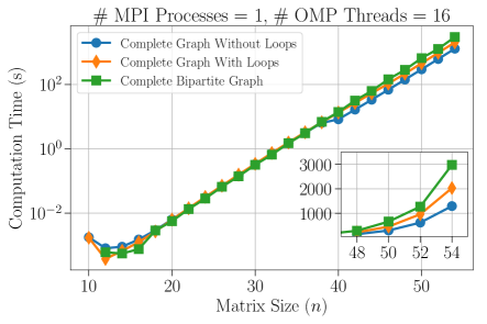
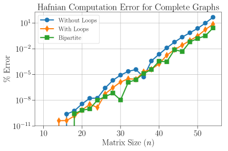
Let us now discuss the results of the numerical implementation of the algorithm. Fig. 3 shows the performance benchmarks for complete and bipartite graphs by varying the size of the matrix (i.e., the number of vertices in the associated graph), using a single MPI process and 16 OpenMP threads for shared memory parallelism. The left panel shows the total computation time in seconds and the right panel shows the scaling of the percentage error defined as
| (4.32) |
where and refer to numerical and analytical results respectively.
The computation time scales exponentially with matrix size (the plots have logscale on the vertical axis) for all types of graphs including complete and bipartite graphs. As shown in the inset, for a complete graph without loops of size it takes approximately 1000 sec. For a graph with loops and a bipartite graph of the same size, the computation times are 2000 sec and 3000 sec respectively. Note that the exponential behaviour is only apparent for . For small the program spends more time in preprocessing and setting up the computation which is responsible for a knee-like behaviour around . By fitting the time scaling with the function for , we obtain and which is the expected scaling behaviour. The overall prefactor sec.
Note that to compute the Hafnian function we need to perform floating point operations and each operation is associated with a small numerical error. We use the standard LAPACK linear algebra package for the computation of the eigenvalues of the submatrices appearing in Eq. (3.28), which is limited to at most double precision. As grows, the number of operations scales exponentially and so does the numerical error in the computation. The right panel of Fig. 3 shows the scaling of the percentage error in the computation (defined as in Eq. 4.32). For , the number of operations is , which comes with an error as large as for a complete graph without loops, for a graph with loops and for bipartite graphs.
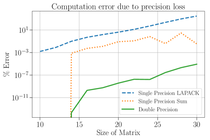
There are two main sources of numerical errors: (i) limited precision of LAPACK, (ii) loss of precision in the numerical sum of an exponentially large number of elements. We distinguish these sources in Fig. 4, by comparing the errors in the Hafnian calculation for a complete graph in the following three settings: (i) Using single precision LAPACK followed by casting the results to double precision and performing the sum in double precision (blue dashed curve), (ii) Using LAPACK in double precision followed by casting the results to single precision and performing the sum in single precision (orange dotted curve), and (iii) Using double precision for both LAPACK and the sum (green solid curve). Clearly, the error due to low precision in LAPACK dominates the low precision summation error. When both tasks are performed in double precision (in the third setting), errors are the lowest. This indicates that the computation errors can be controlled much better if quadruple precision is used for both tasks.
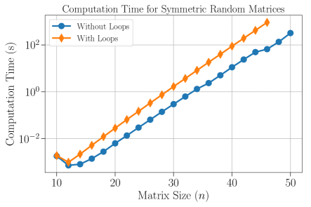
To test the scaling of the computation time, we also consider complex symmetric random matrices of various sizes in Fig. 5. The real and imaginary parts of each element of the matrix are randomly chosen from a uniform distribution and then the resulting matrix is symmetrized. We find that similarly to the case of complete graphs (with matrix elements all being 1), the computation time scales exponentially with . Moreover, since the loop hafnian function requires additional computations associated with the diagonal elements, the computation for those is larger as compared to the hafnian function. For a random matrix with , the computation time is sec and sec for loop hafnian and hafnian respectively with 16 OpenMP threads. For a fixed size the computation times of random matrices are larger than those for matrices corresponding to complete graphs. This is because of the high symmetry of complete graphs which maps to a very simple structure of the eigenvalues of their adjacency matrices.
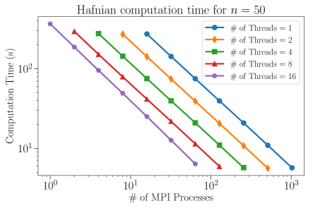
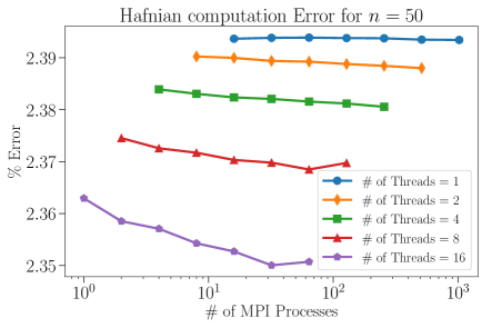
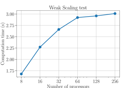
So far, we have only used shared memory parallelism on a single node computer using OpenMP multi-threading. We will now consider a hybrid CPU parallelism: distributing the computation over multiple nodes with OpenMP threads of their own. The time scaling using this hybrid approach for a matrix of size is shown in the left panel of Fig. 6. We consider a range of MPI processes each with varying number of OpenMP threads. The computation turns out to perform extremely well with increasing number of MPI processes. The scaling is almost perfect, i.e. increasing MPI processes by a factor of 2 cuts down the computation time almost by a factor of half. Further enhancement in the computation time can be obtained by harnessing the power of GPU computing, which is beyond the scope of this implementation and is left for future work. Note that numerical summation over multiple processors is a non-commutative process. Therefore, it is expected that when distributing the summation over multiple MPI and OpenMP processors can result in slightly different results. In order to test that, we compute the associated percentage error in computation which is shown in the right panel of Fig. 6. It turns out that choosing different combinations of MPI and OpenMP processes have negligible effect on the accuracy of the results. Using GPUs or other vectorized computing techniques, one may be able to reduce the overall prefactor in the computation time scaling, but that leaves the exponential scaling shown in left panel of Fig. 3 unaffected. Fig. 7 shows the weak scaling test performed by doubling the number of MPI processes while increasing the size of the matrix by 2 each time. We consider matrix sizes which corresponds to problem size and the number of MPI processes considered each having 16 OpenMP threads. Hence, the ratio of the problem size to the number of processors is fixed to . The total computation time plateaus as the processor count increases. This indicates a good weak scaling of the algorithm for larger processor count.
5 Summary
From the discussion above, it is clear that evaluating hafnians of large matrices is limited by two factors: (i) speed and (ii) accuracy. For instance a hafnian computation would take for and for with 16 processors running in parallel. Utilizing all the 18000 CPU nodes (where each node has 16 CPUs, for a total of 288000 CPUs) of the Titan supercomputer and assuming perfect scaling over distributed nodes, computation of a single hafnian would take at least 1.5 months. This severely constrains the size of the problems where one needs to exactly compute many hafnians of large matrix sizes. For example, generating an (exact) sample for Gaussian Boson Sampling would likely require the evaluation of at least one hafnian of the size of the number of events that are sampled (i.e., the number of detectors that click). The above estimation shows that this problem becomes computationally intractable as the number of inputs on the linear interferometer is increased beyond a few tens. One can hope that for a problem of such extent, an ideal quantum device for Gaussian Boson Sampling may generate a sample in a much smaller time scale hence outperforming classical supercomputers.
As future work, it would be interesting to use GPUs as a way to speed up the calculation of hafnians. Progress in the bulk evaluation of the decompositions of real non-symmetric matrices has been presented by Tokura et al. in Ref. [40]. However, for our purpose significant care is needed in sorting out the sizes of the different elements of the powerset sum required to evaluate the hafnian; moreover one would also need to extend the results of Tokura et al. to complex non-hermitian matrices.
6 Acknowledgements
B.G. and N.Q. thank J.M. Arrazola, J. Izaac, H. Jasim, N. Killoran, P. Rebentrost and C. Weedbrook for useful discussions and valuable feedback. This research used resources of the Oak Ridge Leadership Computing Facility at the Oak Ridge National Laboratory, which is supported by the Office of Science of the U.S. Department of Energy under Contract No. DE-AC05-00OR22725.
References
- [1] Alexander Barvinok. Combinatorics and complexity of partition functions, volume 274. Springer, 2016.
- [2] Haruo Hosoya. Topological index. a newly proposed quantity characterizing the topological nature of structural isomers of saturated hydrocarbons. Bulletin of the Chemical Society of Japan, 44(9):2332–2339, 1971.
- [3] Nicolás Quesada. Franck-condon factors by counting perfect matchings of graphs with loops. J. Chem. Phys., 150(16):164113, 2019.
- [4] Leslie G Valiant. The complexity of computing the permanent. Theoretical computer science, 8(2):189–201, 1979.
- [5] Herbert John Ryser. Combinatorial mathematics. Number 14. Mathematical Association of America; distributed by Wiley [New York, 1963.
- [6] E. Bax and J. Franklin. A finite-difference sieve to compute the permanent. Caltech-CS-TR-96-04, California Institute of Technology, 1996.
- [7] K. Balasubramanian. Combinatorics and diagonals of matrices. Ph.D. Thesis, Department of Statistics, Loyola College, Madras, India, T073, Indian Statistical Institute, Calcutta, 1980.
- [8] Junjie Wu, Yong Liu, Baida Zhang, Xianmin Jin, Yang Wang, Huiquan Wang, and Xuejun Yang. A benchmark test of boson sampling on tianhe-2 supercomputer. National Science Review, 5(5):715–720, 2018.
- [9] Alexander Barvinok. Polynomial time algorithms to approximate permanents and mixed discriminants within a simply exponential factor. Random Structures & Algorithms, 14(1):29–61, 1999.
- [10] Alexander Barvinok. Approximating permanents and hafnians. arXiv preprint arXiv:1601.07518, 2016.
- [11] Mark Rudelson, Alex Samorodnitsky, Ofer Zeitouni, et al. Hafnians, perfect matchings and gaussian matrices. The Annals of Probability, 44(4):2858–2888, 2016.
- [12] Steve Chien. A determinant-based algorithm for counting perfect matchings in a general graph. In Proceedings of the Fifteenth Annual ACM-SIAM Symposium on Discrete Algorithms, SODA ’04, pages 728–735, Philadelphia, PA, USA, 2004. Society for Industrial and Applied Mathematics.
- [13] Piotr Sankowski. Alternative algorithms for counting all matchings in graphs. In Helmut Alt and Michel Habib, editors, STACS 2003, pages 427–438, Berlin, Heidelberg, 2003. Springer Berlin Heidelberg.
- [14] Marek Cygan and Marcin Pilipczuk. Faster exponential-time algorithms in graphs of bounded average degree. Information and Computation, 243:75–85, 2015.
- [15] Scott Aaronson and Alex Arkhipov. The computational complexity of linear optics. In Proceedings of the forty-third annual ACM symposium on Theory of computing, pages 333–342. ACM, 2011.
- [16] Alex Neville, Chris Sparrow, Raphaël Clifford, Eric Johnston, Patrick M Birchall, Ashley Montanaro, and Anthony Laing. Classical boson sampling algorithms with superior performance to near-term experiments. Nature Physics, 13(12):1153, 2017.
- [17] Peter Clifford and Raphaël Clifford. The classical complexity of boson sampling. In Proceedings of the Twenty-Ninth Annual ACM-SIAM Symposium on Discrete Algorithms, pages 146–155. SIAM, 2018.
- [18] Craig S Hamilton, Regina Kruse, Linda Sansoni, Sonja Barkhofen, Christine Silberhorn, and Igor Jex. Gaussian boson sampling. Physical review letters, 119(17):170501, 2017.
- [19] Regina Kruse, Craig S Hamilton, Linda Sansoni, Sonja Barkhofen, Christine Silberhorn, and Igor Jex. A detailed study of gaussian boson sampling. arXiv preprint arXiv:1801.07488, 2018.
- [20] AI Lvovsky. Squeezed light. Photonics Volume 1: Fundamentals of Photonics and Physics, pages 121–164, 2015.
- [21] Alexander I Barvinok. Two algorithmic results for the traveling salesman problem. Mathematics of Operations Research, 21(1):65–84, 1996.
- [22] Aram W Harrow and Ashley Montanaro. Quantum computational supremacy. Nature, 549(7671):203, 2017.
- [23] Nicolás Quesada, Juan Miguel Arrazola, and Nathan Killoran. Gaussian boson sampling using threshold detectors. Phys. Rev. A, 98:062322, 2018.
- [24] Brajesh Gupt, Juan Miguel Arrazola, Nicolás Quesada, and Thomas R Bromley. Classical benchmarking of gaussian boson sampling on the titan supercomputer. arXiv preprint arXiv:1810.00900, 2018.
- [25] Andreas Björklund and Thore Husfeldt. Exact algorithms for exact satisfiability and number of perfect matchings. Algorithmica, 52(2):226–249, 2008.
- [26] Raymond Kan. From moments of sum to moments of product. Journal of Multivariate Analysis, 99(3):542–554, 2008.
- [27] Mikko Koivisto. Partitioning into sets of bounded cardinality. In International Workshop on Parameterized and Exact Computation, pages 258–263. Springer, 2009.
- [28] Jesper Nederlof. Fast polynomial-space algorithms using möbius inversion: Improving on steiner tree and related problems. In International Colloquium on Automata, Languages, and Programming, pages 713–725. Springer, 2009.
- [29] Andreas Björklund. Counting perfect matchings as fast as ryser. In Proceedings of the twenty-third annual ACM-SIAM symposium on Discrete Algorithms, pages 914–921. SIAM, 2012.
- [30] Grzegorz Rempala and Jacek Wesolowski. Symmetric functionals on random matrices and random matchings problems, volume 147. Springer Science & Business Media, 2007.
- [31] Donald E. Knuth. The Art of Computer Programming, Vol. 2: Seminumerical Algorithms. Addison-Wesley, 3 edition, 1998.
- [32] Milton Abramowitz and Irene A Stegun. Handbook of mathematical functions: with formulas, graphs, and mathematical tables, volume 55. Dover, 1972.
- [33] Thore Husfeldt. Invitation to algorithmic uses of inclusion–exclusion. In International Colloquium on Automata, Languages, and Programming, pages 42–59. Springer, 2011.
- [34] Roger A Horn, Roger A Horn, and Charles R Johnson. Matrix analysis. Cambridge university press, 1990.
- [35] Edward Anderson, Zhaojun Bai, Christian Bischof, L Susan Blackford, James Demmel, Jack Dongarra, Jeremy Du Croz, Anne Greenbaum, Sven Hammarling, Alan McKenney, et al. LAPACK Users’ guide. SIAM, 1999.
- [36] I-Li Lu and Donald St P Richards. Macmahon’s master theorem, representation theory, and moments of wishart distributions. Advances in Applied Mathematics, 27(2-3):531–547, 2001.
- [37] Matjaz Konvalinka and Igor Pak. Non-commutative extensions of the macmahon master theorem. arXiv preprint math/0607737, 2006.
- [38] hafnian. https://github.com/XanaduAI/hafnian, 2018.
- [39] Nathan Killoran, Josh Izaac, Nicolás Quesada, Ville Bergholm, Matthew Amy, and Christian Weedbrook. Strawberry Fields: A Software Platform for Photonic Quantum Computing. Quantum, 3:129, 2019.
- [40] Hiroki Tokura, Takumi Honda, Yasuaki Ito, Koji Nakano, Mitsuya Nishino, Yushiro Hirota, and Masami Saeki. An efficient gpu implementation of bulk computation of the eigenvalue problem for many small real non-symmetric matrices. International Journal of Networking and Computing, 7(2):227–247, 2017.
- [41] Arne Storjohann. An o (n 3) algorithm for the frobenius normal form. In ISSAC, volume 98, pages 101–104. Citeseer, 1998.
- [42] Mark Giesbrecht. Nearly optimal algorithms for canonical matrix forms. SIAM Journal on Computing, 24(5):948–969, 1995.
- [43] Walter Keller-Gehrig. Fast algorithms for the characteristics polynomial. Theoretical computer science, 36:309–317, 1985.
- [44] Max Neunhöffer and Cheryl E Praeger. Computing minimal polynomials of matrices. LMS Journal of Computation and Mathematics, 11:252–279, 2008.
A Number of elements in SPM()
For even one can obtain a closed form expression for the number of elements in SPM(). Consider first PMP the set of perfect matchings in a graph with vertices. One can start breaking pairs, i.e., taking a matching such as and turn into two loops . If one “breaks” pairs there are ways of doing this for each perfect matching. However this will overcount the number of partitions. For example if one breaks every matching of the following three perfect matchings , and one will always get the same set of loops thus one needs to account for multiple counting by dividing by the factor . We conclude that if one breaks pairs from the set of perfect matching of objects one gets partitions. We now need to sum over all possible to obtain the total number of partitions
| (A.1) |
where is the Toronto function and is the Kummer confluent hypergeometric function [32]. We also have the following asymptotic limit and bound:
| (A.2) | |||
| (A.3) |
B Fast calculation of power traces
For the calculation of the hafnian of an matrix it is required to know the quantities
| (B.4) |
This can be done by first obtaining the minimal polynomial of the matrix , which is the monic polynomial of least degree such that = 0. Note that for an matrix the minimal polynomial is at most of degree by the Cayley-Hamilton theorem. Assuming that is the degree of the minimal polynomial we write it as
| (B.5) |
and using the fact that is the minimal polynomial of we write
| (B.6) | ||||
| (B.7) | ||||
| (B.8) |
Thus, once the minimal polynomial is known, one can easily calculate any power trace of degree of a matrix. The minimal polynomial calculation can be done in time where quantifies the complexity of matrix-matrix multiplication [41, 42, 43, 44]. Note that these algorithms only require operations within the field in which the matrix is expressed and are exact in infinite precision arithmetic. Yet, when used in finite precision arithmetic (i.e. in real hardware with finite RAM) these algorithms do not perform better in terms accuracy than a Schur factorization of the matrix followed by exponentiation and summation of the eigenvalues for calculating power traces. The same conclusion holds for the calculation of in Sec. 3.3 and thus we prefer to use the Schur decomposition for the calculation of the power traces.
C Hafnians of low rank matrices
We argue how the hafnian of a matrix that has rank over the field , can be computed in time . This generalizes a result of Barvinok for the permanent [21].
Let be the set of perfect matching permutations on elements, i.e., permutations such that and .
Given a matrix , its hafnian is
| (C.9) |
Note that for any lower triangular matrix ,
| (C.10) |
since the hafnian, as defined above, does only depend on elements above the diagonal.
If we can find a matrix for any lower triangular such that
| (C.11) |
for a small enough , there is a relatively efficient algorithm to compute the hafnian following the permanent algorithm by Barvinok [21], as follows: Introduce indeterminates , and consider the multivariate polynomial
| (C.12) |
Let be the set of integer -partitions of , i.e., tuples such that
-
1.
,
-
2.
.
Let be the subset of of even partitions, i.e., tuples such that also is even for all . Note that
| (C.13) |
Let denote the double factorial of , i.e., . We use the convention that for is . The hafnian can now be expressed in the coefficients of as
| (C.15) |
Given the coefficients , this can be evaluated in time. Note that since we only need the coefficients for , it is interesting to investigate if there are faster ways to obtain these than computing all of (C.14) explicitly.