Microlocal analysis of
Doppler Synthetic Aperture Radar

Abstract.

We study the existence and suppression of artifacts for a Doppler-based Synthetic Aperture Radar (DSAR) system. The idealized air- or space-borne system transmits a continuous wave at a fixed frequency and a co-located receiver measures the resulting scattered waves; a windowed Fourier transform then converts the raw data into a function of two variables: slow time and frequency. Under simplifying assumptions, we analyze the linearized forward scattering map and the feasibility of inverting it via filtered backprojection, using techniques of microlocal analysis which robustly describe how sharp features in the target appear in the data. For DSAR with a straight flight path, there is, as with conventional SAR, a left-right ambiguity artifact in the DSAR image, which can be avoided via beam forming to the left or right. For a circular flight path, the artifact has a more complicated structure, but filtering out echoes coming from straight ahead or behind the transceiver, as well as those outside a critical range, produces an artifact-free image. We show that these results are qualitatively robust; although initially derived under an approximation widely used for range-based SAR, they are either structurally stable or robust with respect to a more accurate model.

Raluca Felea

School of Mathematical Sciences

Rochester Institute of Technology

Rochester, NY, 14623, USA

Romina Gaburro

Department of Mathematics and Statistics

and Health Research Institute

University of Limerick

Limerick, V94 T9PX, Ireland

Allan Greenleaf

Department of Mathematics

University of Rochester

Rochester, NY, 14627, USA

Clifford Nolan

Department of Mathematics and Statistics

and Health Research Institute

University of Limerick

Limerick, V94 T9PX, Ireland

1. Introduction

Synthetic aperture radar (SAR) systems transmit electromagnetic waves from an airborne or spaceborne antenna, which then scatter from objects of interest on the terrain, e.g., roads, vehicles, buildings or natural features. The scattered waves are measured by a receiver either co-located with the transmitting antenna (monostatic SAR) or on one or more other platforms (bi- or multi-static). Radar transmitters operate in a variety of modes, with the emitted waves ranging from wideband pulses to ultra-narrowband, continuous wave (CW) signals. The Doppler Synthetic Aperture Radar (DSAR) system we analyze in this paper is of the latter type, with narrow temporal windowing superimposed on the received scattered waves generated by a single frequency transmitted wave. (This approach to applying temporal windows to CW signals has some similarity to what is known as pseudo-pulse processing in the radar literature, which has been used previously for SAR [34].) Possible uses of DSAR include low power applications and imaging through media which are either dispersive or have frequency-dependent attenuation.

The narrowband nature of the DSAR waveforms allows accurate measurement of Doppler frequency shifts, which in turn can be used to obtain accurate measurements of relative velocity. Knowledge of relative velocity between stationary scattering objects and the antenna, whose trajectory is assumed known, is then used to locate and image the objects. The dual concept of using Doppler shifts to image rotating or moving objects, using measurements by a stationary antenna, was proposed some time ago by Thomson and Ponsonby [38]; see also [35]. More recently, the use of a moving antenna over a horizontal terrain was proposed in Borden and Cheney [5]. In Wang and Yazici [40], this approach was named Doppler Synthetic Aperture Radar and examined for bistatic data acquisition; related ideas were further developed in [9, 37, 42, 43, 41, 44]. The reader can also consult these papers for more extensive surveys of the earlier literature.

In contrast to DSAR, in standard SAR the transmitted fields often consist of a train of pulses of short temporal duration and complicated spectrum; the short duration allows for high-resolution estimates of the time between transmitting and receiving antennas (whether in monostatic, bi-static or multi-static geometries), and this travel time is used to estimate the distance (range) between the antenna and the scattering objects. This process is repeated from many locations along the transmitter flight path, providing distance estimates from many different viewing angles, from which both the range and the along-track position of scattering objects can be determined.

In this paper, we study monostatic DSAR using methods of microlocal analysis. Microlocal techniques allow one to develop backprojection algorithms for reconstruction of features on the ground (which we call a scene) up to smooth errors, as well as analyze obstructions to such reconstruction in the form of imaging artifacts (fictitious features in reconstructions of a scene). Such methods have been highly successful in either revealing artifacts, arising in conventional monstatic and bistatic SAR, or in rigorously explaining artifacts that have already been observed. See [12], [30] and [36] for examples of artifacts that are either predicted or explained by microlocal analysis. Also see [13] for an example of how to ameliorate the effects of artifacts. We describe what types of artifacts appear in DSAR and obtain sufficient conditions under which they can be excluded, allowing for robust imaging of sharp features on the ground (such as walls and edges) via filtered backprojection.

For simplicity, we treat the problem of imaging a stationary scene located on a flat terrain. After considering the structure of DSAR for general flight paths, we focus on two model trajectories, namely a straight flight path and a circular one. For these we characterize what artifacts arise in the imaging, and describe criteria for avoiding them (see Sections 6 and 7).

More precisely, in this paper we first use the Born approximation and other approximations to create a forward map $\mathcal{F}$ taking the scene $V(\mathbf{x})$ to be imaged to a windowed Fourier transform $W(s,\omega)$ of the DSAR data. (Here, $\mathbf{x}$ are coordinates on the ground, $s$ is the slow time parametrizing the transceiver’s flight path $\gamma(s)$ (assumed smooth) and $\omega$ denotes frequency.) We then analyze $\mathcal{F}$, showing that it is a Fourier integral operator, and study the implications of its microlocal geometry for imaging by filtered backprojection.

For the linear trajectory, we show in Theorem 2 that there is a left-right artifact, similar to that which arises in monostatic SAR (see Remark 2), and which can be avoided using beam forming to the left or right of the flight track. Furthermore, it is shown in Sec. 8 that this conclusion still holds under a more refined and realistic model, indicating that our conclusions are robust. For a circular flight path, the geometry is different and the artifacts are more complicated (see Remark 7), but in Theorem 3 we are able to precisely characterize the artifacts, and then give criteria for avoiding them (e.g., see (69) in Lemma 5).

2. The Doppler SAR model

We consider an aircraft- or satellite-borne antenna, transmitting a time-harmonic signal $e^{-i\omega_{0}t}$ that scatters off the terrain and is then detected with the same antenna. The received signal is then used to produce an image of the terrain; we follow [5] closely for the initial modeling; in particular we ignore polarization and use the scalar, time-domain wave equation,

(1) $$\left(\nabla^{2}-\frac{1}{c^{2}(\mathbf{y})}\partial^{2}_{t}\right)E(t,\mathbf{y})=f(t,\mathbf{y}),$$

where $\mathbf{y}\in\mathbb{R}^{3}$, $E$ is (one component of the) electric field, $f$ describes the source, and the function $c$ is the wave propagation speed.

For the majority of this paper, we take the source $f$ to be of constant angular frequency, of the form $f(t,\mathbf{y})=e^{-i\omega_{0}t}\delta(\mathbf{y}-\mathbf{\gamma}(t))$, where ${\gamma}:=\left\{\mathbf{\gamma}(t)\>|\>t_{min}<t<t_{max}\right\}$ is the curve describing the antenna flight path. In particular, in this model we assume that the antenna radiates isotropically. More generally, following [8] and [31], we recall below how an explicit antenna beam pattern can be incorporated in $f$, but this will only affect the amplitudes and not the phase function and geometry.

To avoid irrelevant degeneracies, we impose some assumptions,

Assumption 1.

The flight path is strictly above the ground and, in the region between the flight path and the ground, $c(\mathbf{y})=c_{0}$, the constant speed of light in dry air.

We define the reflectivity function, $\frac{1}{c_{0}^{2}}-\frac{1}{c^{2}(\mathbf{y})}$, which encodes changes in the propagation speed. Electromagnetic waves attenuate rapidly as they propagate into the earth, which is modeled by the following assumption:

Assumption 2.

The reflectivity function is of the form $V(\mathbf{y}^{\prime})\delta(y_{3}),\,\mathbf{y}^{\prime}\in\mathbb{R}^{2}$.

We provide below a very brief sketch of the linearized model of the scattered waves and we refer the reader to [31] for more details. If we formally linearize (1) by writing $c=c_{0}+\delta c,E=E_{0}+\delta E$, then the scattered field, $\delta E$, approximately satisfies

(2) $$\left(\nabla^{2}-\frac{1}{c^{2}(\mathbf{y})}\partial^{2}_{t}\right)\delta E(t,\mathbf{y})=-V(\mathbf{y},t)\partial_{t}^{2}E_{0}(t,\mathbf{y})$$

where the incident field, $E_{0}$, satisfies (1) with $c$ replaced by $c_{0}$. This is the Born approximation of the scattered field. If we wish to include an antenna beam pattern in (1), we set $f(t,\mathbf{y})=J_{s}(\mathbf{y})e^{-i\omega_{0}t}$, where $J_{s}(\mathbf{y})$ is related to the current distribution on the antenna.

Finally, for the time being, we make the following simplifying assumption:

Assumption 3.

Start-stop approximation: The speed of wave propagation is so large, relative to the motion of the transceiver along $\gamma$, that the point where the wave is detected by the receiver after scattering off the terrain is the same as where the transmitter emitted it.

The start-stop approximation is common in range-based SAR. There, the emitted wave consists of a chain of short duration pulses and, at least for airborne systems, the speed of the platform is small relative to the speed of light; see [39, 7] for further discussion. In our setup, the start-stop approximation at first glance seems much harder to justify: rather than using short duration pulses (typically with complex spectra), it uses a long duration/narrow bandwidth signal, idealized as continuous wave (CW). We make this assumption because the calculations needed for the microlocal techniques used become far more complicated without it. However, we are able to partially justify the start-stop approximation for DSAR, ex post facto, by showing that the canonical relations associated to the linearized forward scattering map are either structurally stable (in the case of a circular flight path) or robust to a first-order correction (in the case of a linear flight path, as shown in Sec. 8).

For $\mathbf{x}\in\mathbb{R}^{2}$, let

(3) $$\mathbf{R}(t):=(\mathbf{x},0)-\mathbf{\gamma}(t)\quad\textnormal{and}\quad R(t):=|\mathbf{R}(t)|.$$

The start-stop approximation yields the total time of travel for a transmitted wave, $T_{tot}$, as follows: the downward travel time of the wave emitted at time $t_{tr}=t$ from $\mathbf{\gamma}(t)$ to $\mathbf{x}$ is $c_{0}^{-1}R(t)$; the wave is thus incident to $\mathbf{x}$ at time $t_{in}=t+c_{0}^{-1}R(t)$. The scattered wave is then detected by the receiver at time $t_{sc}=t+T_{tot}$, with $T_{tot}$ determined implicitly by

(4) $$c_{0}T_{tot}=R(t)+R\left(t+T_{tot}\right).$$

Under the start-stop approximation, we have $R\left(t+T_{tot}\right)=R(t)$ and thus $T_{tot}\approx 2c_{0}^{-1}R(t)$. (This calculation will be refined in Sec. 8.) Using the assumptions above and the Green’s function for the wave equation,

(5) $$G(t,{\mathbf{y}})={\delta(t-|{\mathbf{y}}|/c)\over 4\pi|{\mathbf{y}}|},$$

convolving $G$ with $f$ to get $E_{0}$ and then convolving $G$ with the right-hand side of (2), we see that under the stop-start approximation, the scattered wave measured on the antenna is

(6) $$d(t):=\delta E(t,\gamma(t))\approx\int_{\mathbb{R}^{2}}\frac{e^{-i\omega_{0}\left(t-2R\left(t\right)/c_{0}\right)}}{\left(4\pi R\left(t\right)\right)^{2}}\ p(\mathbf{x},\omega)V(\mathbf{x})d\mathbf{x}.$$

The amplitude $p(\mathbf{x},\omega)$ is related to $J_{s}$ and is the antenna beam pattern, referring to the fact that one can phase the individual elements of the antenna to interfere in such a way as to selectively illuminate desired parts of the scene on the ground. Note that a further refinement is also possible with regard to beam-forming on the received signal [31]. For the majority of our discussion, the beam pattern is not important and unless otherwise stated, we take $p\equiv 1$ in (6).

Note also that, for ease of notation, we suppress the dependence of $\mathbf{R}$ and $R$ on $x$. Furthermore, the slowly varying range factor in the denominator of (6), as well as any constants, will be absorbed into the amplitude $a$ in (10) below.

The Doppler problem, like most radar problems, involves multiple time scales. The speed of light is $c_{0}\approx 3\cdot 10^{8}$ m/sec, whereas aircraft speeds are typically subsonic, or less than about $3\cdot 10^{2}$ m/sec. Even satellites in low earth orbit travel only on the order of 8 km/sec $\approx 10^{4}$ m/sec. Moreover, the frequencies involved are usually very large, typically above 1 GHz $=10^{9}$ Hertz. To analyze the signal (6), we introduce a “slow time” $s$, and multiply the data by a windowing function, whose duration is (i) small relative to the antenna motion (i.e., the distance the antenna travels during the window is small relative to a wavelength), but (ii) large enough so that the transmitted signal undergoes a sufficiently large number of cycles over the support of the window so as to be amenable to Fourier analysis. We take the window about $t=s$ to be of the form $\ell\left(\omega_{0}\left(t-s\right)\right)$, where $\ell(t)$ is smooth, identically equal to 1 for $|t|\leq L$ and supported in $|t|\leq 2L$, for some appropriately chosen $L>0$. Although of compact support, it is natural to consider $\ell(\cdot)$ as being a symbol of order zero (see below), as the functions $\ell(\omega_{0}\cdot)$ are symbols of order 0 uniformly in $\omega_{0}$ and $L$.

Computing the resulting windowed Fourier transform of the data, localizing near $s$ in the time variable and using $\omega$ for the frequency variable, we form

$$W_{0}(s,\omega) :=\int e^{i\omega(t-s)}\ell(\omega_{0}(t-s))d(t)dt$$

(7) $$=\int e^{i\omega(t-s)}\ell(\omega_{0}(t-s))\int\frac{e^{-i\omega_{0}\left(t-2R\left(t\right)/c_{0}\right)}}{\left(4\pi R\left(t\right)\right)^{2}}V(\mathbf{x})d\mathbf{x}dt$$

In (2) we Taylor expand $R(t)$ about $t=s$ (cf. [5, Eqns. (7-8)]) as

(8) $$R(t)=R(s)+\dot{R}(s)(t-s)+\cdots,$$

using the convention throughout that dot denotes differentiation with respect to time. Keeping only the linear terms then results in the approximation of $W_{0}$ which will be the object of study:

(9) $$W(s,\omega) :=\int e^{i\omega(t-s)}\ell(\omega_{0}(t-s))\int\frac{e^{-i\omega_{0}\left(t-2\left(R\left(s\right)+\dot{R}(s)(t-s)\right)/{c_{0}}\right)}}{(4\pi R(s))^{2}}V(\mathbf{x})d\mathbf{x}dt.$$

After the change of variables $t\mapsto\tau=t-s$, this becomes

(10) $$W(s,\omega) =\int e^{i\omega\tau}\ell(\omega_{0}\tau)\int\frac{e^{-i\omega_{0}(s+\tau-2(R(s)+\dot{R}(s)\tau)/c_{0})}}{(4\pi R(s))^{2}}V(\mathbf{x})d\mathbf{x}d\tau$$

$$=\int e^{i\tau(\omega-\omega_{0}+2\omega_{0}\dot{R}/c_{0})}\underbrace{(\ell(\omega_{0}\tau)e^{i\omega_{0}\left(2R\left(s\right)/c_{0}-s\right)})/((4\pi R(s))^{2})}_{a(s,\omega_{0},\mathbf{x};\tau)}d\tau\,V(\mathbf{x})d\mathbf{x}$$

We define the DSAR transform by $\mathcal{F}:V(\mathbf{x})\to W(s,\omega)$, and show below that from the form (10) one can identify $\mathcal{F}$ as a Fourier integral operator (FIO). Although not stated explicitly in (10), we will implicitly assume that $W$ has been multiplied by a smooth cut-off function with compact support. This makes physical sense but also is necessary to avoid artifacts in the backprojected image later on. We will describe the main ideas and results on FIOs and other aspects of microlocal analysis as needed, but also refer the reader to [10, 23, 25] for more detailed accounts.

3. The DSAR transform as a Fourier Integral Operator

A Fourier integral operator (FIO) is an integral operator whose kernel has the form $K(\mathbf{y},\mathbf{x})=\int e^{i\phi(\mathbf{y},\mathbf{x},\tau)}a(\mathbf{y},\mathbf{x};\tau)d\tau$, where the phase $\phi$ and amplitude $a$ satisfy certain conditions outlined below. In our case, the output variables are $\mathbf{y}=(s,\omega)$; the input variables are the components of $\mathbf{x}$; $a$ is as in (10); and $\phi(\mathbf{y},\mathbf{x})=\tau(\omega-\omega_{0}+2\omega_{0}\dot{R}/c_{0})$.

Theorem 1.

Under assumptions 1 and 2, the mapping $\mathcal{F}$ is a Fourier integral operator of order $-1/2$ associated with the canonical relation $\mathcal{C}$ in (15) below.

Proof.

To check that $\mathcal{F}$ given by (10) is an FIO, we need to check the following conditions on the amplitude and phase of (10).

First, the phase $\phi(s,\omega,\mathbf{x};\tau):=\tau(\omega-\omega_{0}+2\omega_{0}\dot{R}(s)/c_{0})$ is an operator phase function in the sense of Hörmander [23], meaning that its differential in all the variables,

(11) $$d_{s,\omega,\mathbf{x},\tau}\phi=\left(\tau 2\omega_{0}\ddot{R}(s)/c,\tau,2\tau\omega_{0}d_{\mathbf{x}}\dot{R}(s)/c_{0},\omega-\omega_{0}+2\omega_{0}\dot{R}(s)/c_{0}\right),$$

is nonzero for $\tau\neq 0$. This is easily checked.

Second, the amplitude $a(s,\omega,\mathbf{x};\tau)$ must satisfy certain symbol estimates. We note first that the function $\ell(\omega_{0}\tau)$ is a symbol of order 0 in the phase variable $\tau$, which means that it belongs to the class

(12) $$S^{0}_{1,0}=\big{\{}b(s,\omega,\mathbf{x};\tau):\left|\partial^{\alpha}_{s,\omega,\mathbf{x}}\partial_{\tau}^{j}b\right|\leq C_{\alpha j}\left(1+\left|\tau\right|\right)^{-j}\quad\forall j\in\mathbb{N},\,\alpha\in\mathbb{N}^{5}\big{\}},$$

where $\partial^{\alpha}_{s,\omega,\mathbf{x}}=\partial_{s}^{\alpha_{1}}\partial_{\omega}^{\alpha_{2}}\partial_{x_{1}}^{\alpha_{3}}\partial_{x_{2}}^{\alpha_{4}}\partial_{x_{3}}^{\alpha_{5}}$ and $\mathbb{N}$ denotes the nonnegative integers. Moreover, since the amplitude $a$ is a product of a smooth, nonzero function of $(s,\mathbf{x})$, independent of $\omega$ and $\tau$, with the order 0 symbol $\ell(\omega_{0}\tau)$, $a$ is also a symbol of order 0, i.e., its derivatives satisfy (12) with $\ell(\omega_{0}\tau)$ replaced by $a(s,\omega,\mathbf{x};\tau)$.

Note that, since $\ell(\cdot)$ is of compact support, so is $a$ (as a function of $\tau$). Thus, $\mathcal{F}$ is strictly speaking a smoothing operator; however, in order to understand how singularities in the reflectivity function are transformed into the data, we consider $a$ as a symbol of order 0, which is uniform in $\omega_{0}$ and $L$, as mentioned above. Note also that $a$ is of compact support in the spatial variables, since we assume that the antenna is compactly supported.

Finally, the order of the operator comes from the Hörmander convention for the orders of FIOs [23]:

(13) $$\hbox{order}(\mathcal{F}) =\hbox{order}(a)+\frac{\#\hbox{phase vars}}{2}-\frac{\#\hbox{output vars}+\#\hbox{input vars}}{4}$$

(14) $$=0+\frac{1}{2}-\frac{2+2}{4}=-\frac{1}{2}.$$

This completes the proof of Theorem 1.

∎

The properties of an FIO involve the geometry of certain key sets. The first is called the critical manifold of $\phi$, which for $\mathcal{F}$ is defined by

$$Crit_{\phi}=\left\{(s,\omega,\mathbf{x},\tau):d_{\tau}\phi=\omega-\omega_{0}+2\omega_{0}\dot{R}(s)/c_{0}=0\right\}.$$

Because $\phi$ is nondegenerate in the sense that the full gradient of $d_{\tau}\phi$ in all the variables is nonzero, it follows that $Crit_{\phi}$ is a smooth, codimension one surface.

In general, a nondegenerate phase function determines, in addition to $Crit_{\phi}$, a second key set, $\mathcal{C}$, called the (twisted) canonical relation of $\phi$ (or $\mathcal{F}$), which is a smooth, immersed submanifold of the total cotangent space of all the variables, both input and output. The canonical relation describes microlocally how $\mathcal{F}$ transforms the locations and directions of singularities in the input variables (i.e., of the reflectivity $V$) to singularities in the output variables (i.e., of the signal $d$). Examples of canonical relations include, but are not limited to, the graphs of canonical transformations between the cotangent spaces of the the input and output variables.

The twisted canonical relation $\mathcal{C}$ is the image of $Crit_{\phi}$ under the map

$$(s,\omega,\mathbf{x},\tau)\in Crit_{\phi}\longrightarrow(s,\omega,d_{s}\phi,d_{\omega}\phi;\mathbf{x},-d_{\mathbf{x}}\phi)\in T^{*}\mathbb{R}^{2}\times T^{*}\mathbb{R}^{2}.$$

Here $T^{*}\mathbb{R}^{2}$ denotes the cotangent bundle of $\mathbb{R}^{2}$, which for the purpose of calculations can be considered as simply $\mathbb{R}^{4}$. With respect to the coordinates $(s,\omega,\sigma,\Omega;\mathbf{x},\mathbf{\xi})$ on $T^{*}\mathbb{R}^{2}\times T^{*}\mathbb{R}^{2}$, $\mathcal{C}$ can be written as

(15) $$\mathcal{C} =\left\{(s,\omega,d_{s}\phi,d_{\omega}\phi;\mathbf{x},-d_{\mathbf{x}}\phi)|_{Crit_{\phi}}\right\}$$

(16) $$=\left\{\left(s,\omega_{0}-2\omega_{0}\dot{R}/c_{0},2\omega_{0}\tau\ddot{R}/c_{0},\tau;\mathbf{x},\underbrace{-2\tau\omega_{0}d_{\mathbf{x}}\dot{R}/c_{0}}_{\bm{\xi}}\right):s\in\mathbb{R},\mathbf{x}\in\mathbb{R}^{2},\tau\in\mathbb{R}\setminus 0\right\}$$

(17) $$\subset(T^{*}\mathbb{R}^{2}\setminus\mathbf{0})\times(T^{*}\mathbb{R}^{2}\setminus\mathbf{0}).$$

Here, $\mathbf{0}$ denotes the zero section of $T^{*}\mathbb{R}^{2}$, namely $\{(\sigma,\Omega)=(0,0)\}$ and $\mathbf{\xi}=\{(0,0)\}$, resp. Since both $\omega_{0}\neq 0$ and $\tau\neq 0$, the claim above that $\mathcal{C}$ does not intersect the zero section of either factor space follows from Remark 1 in Sec. 5 below. From (15), one sees that $x,s,\tau$ are coordinates on $C$, which we will use for calculations.

In summary, $\mathcal{F}$ is an FIO of order $-1/2$ associated with $\mathcal{C}$, denoted by $\mathcal{F}\in I^{-\frac{1}{2}}(\mathcal{C})$. In later sections, we study the projections from the canonical relation $\mathcal{C}$ to the two factor spaces $T^{*}\mathbb{R}^{2}$ on the left and right. The left projection $\pi_{L}:\mathcal{C}\rightarrow T^{*}\mathbb{R}^{2}$ is defined by

(18) $$\pi_{L}:(s,\omega,\sigma,\tau;\mathbf{x},\bm{\xi})\mapsto(s,\omega,\sigma,\tau),$$

while the right projection $\pi_{R}:\mathcal{C}\rightarrow T^{*}\mathbb{R}^{2}$ is given by

(19) $$\pi_{R}:(s,\omega,\sigma,\tau;\mathbf{x},\bm{\xi})\mapsto(\mathbf{x},\bm{\xi}).$$

Understanding these projections gives us information about the geometry of $\mathcal{C}$ and thus the properties of $\mathcal{F}$. The next subsection gives the background needed for the subsequent analysis.

3.1. The left and right projections and the Bolker condition

It is a basic aspect of microlocal analysis that, for a general canonical relation, the singularities of the projections $\pi_{L}$ and $\pi_{R}$, in the sense of $C^{\infty}$ singularity theory [18], e.g., points where their differentials have less than maximal rank, have important implications for the operator theory of associated FIOs. In particular, in applications to inverse problems via the study of linearized forward maps, the singularities of $\pi_{L}$ and $\pi_{R}$ determine whether reconstruction via filtered backprojection (modulo smooth errors) is possible, and allows the characterization of artifacts cf. [32, 11, 15, 17, 1, 14, 33, 16, 2].

For any canonical relation, say $\mathcal{C}_{0}\subset T^{*}\mathbb{R}^{n}\times T^{*}\mathbb{R}^{n}$ associated with an FIO $\mathcal{F}_{0}$, if one of the two maps $D\pi_{L}$ and $D\pi_{R}$ is nonsingular at a point $\lambda\in\mathcal{C}_{0}$, then so is the other. These derivatives $D\pi_{L}$ and $D\pi_{R}$ are each represented by a $(2n)\times(2n)$ matrix, so the nonsingularity condition takes either of the forms,

(20) $$\det(D\pi_{L})(\lambda)\neq 0\hbox{ if and only if }\det(D\pi_{R})(\lambda)\neq 0.$$

We denote by $\Sigma$ the set

$$\Sigma=\left\{\lambda_{0}\in\mathcal{C}_{0}:\det(D\pi_{R}(\lambda_{0}))=0\right\}.$$

If $\Sigma=\emptyset$, we say that $\mathcal{C}_{0}$ is nondegenerate; otherwise, it is degenerate. If the complement of $\Sigma$ contains a sufficiently small neighborhood of $\lambda_{0}$, i.e. the determinant of (20) is nonzero in a neighborhood of $\lambda_{0}$, then $\mathcal{C}_{0}$ is a local canonical graph near $\lambda_{0}=(y_{0},\eta_{0},x_{0},\xi_{0})$ in the sense that $\mathcal{C}_{0}$ is the graph of a canonical transformation $\chi:T^{*}\mathbb{R}^{n}\to T^{*}\mathbb{R}^{n}$ defined near $(x_{0},\xi_{0})$. See, e.g., [23], [24, Thm. 21.2.14].

Even though $D\pi_{L}$ and $D\pi_{R}$ drop rank on the same set, and their kernels have the same dimension, the maps $\pi_{L}$ and $\pi_{R}$ may have different types of singularities.

Backprojection methods attempt to form an image by applying the adjoint $\mathcal{F}_{0}^{*}$ to the data $\mathcal{F}_{0}V$. If $\mathcal{C}_{0}$ is a local canonical graph, the formation of the composition $\mathcal{F}_{0}^{*}\mathcal{F}_{0}$ is covered by the transverse intersection calculus for FIOs [23, 25, 10], resulting in $\mathcal{F}_{0}^{*}\mathcal{F}_{0}\in I^{2m}(\mathcal{D})$ with $\mathcal{D}$ a canonical relation containing part of the diagonal relation, $\Delta:=\{(\mathbf{x},\mathbf{\xi},\mathbf{x},\mathbf{\xi}):(\mathbf{x},\mathbf{\xi})\in T^{*}\mathbb{R}^{n}\setminus 0\}$ [25, §25.2-3]. If the canonical relation $\mathcal{D}$ contains only points of the diagonal $\Delta$, then $\mathcal{F}_{0}^{*}\mathcal{F}_{0}$ is a pseudodifferential operator. In this case, under an illumination assumption, one can construct a left parametrix for $\mathcal{F}_{0}^{*}\mathcal{F}_{0}$, i.e., a pseudodifferential operator $Q$ of order $-2m$ satisfying $Q\mathcal{F}_{0}^{*}\mathcal{F}_{0}=I$ up to a smoothing operator ( assuming that $F^{*}F$ is elliptic). This means that $Q\mathcal{F}_{0}^{*}$ is a filtered backprojection operator that allows us to reconstruct a function $V(\mathbf{x})$ from the data $\mathcal{F}_{0}V$, up to a smooth error. Any sharp features in $V(\mathbf{x})$ (such as discontinuities or edges) that are visible in the data will be present in the image, and vice versa; we say that there are no artifacts in the reconstruction.

If, on the other hand, $\mathcal{D}$ contains off-diagonal points, not in the diagonal $\Delta$, using straightforward backprojection reconstruction results in artifacts, i.e., spurious features in the image which are not present in the original scene. This is prevented if the Bolker condition [20] is satisfied, which in the DSAR setting reduces to

(21) $$(i) \Sigma=\emptyset\hbox{ (i.e., the projections are nonsingular everywhere);}$$

(22) $$(ii) \pi_{L}\hbox{ is one-to-one (injective).}$$

An injectivity condition on $\pi_{L}$ such as (ii) is natural for the prevention of artifacts, since injectivity implies that different points in the scene correspond (microlocally) to different points in the data, while (i) implies that the standard transverse intersection calculus of FIO applies to the composition $\mathcal{F}_{0}^{*}\mathcal{F}_{0}$. When combined into the Bolker condition (21), these ensure that $\mathcal{D}\subset\Delta$, that $\mathcal{F}_{0}^{*}\mathcal{F}_{0}$ is a pseudodifferential operator, and that there are no artifacts in reconstructions made using $\mathcal{F}_{0}^{*}$.

4. Contributions of this paper

We have shown above that the DSAR operator $\mathcal{F}$ is an FIO and consequently can be analyzed by the techniques of microlocal analysis. In the remainder of this paper, we analyze the geometry of the canonical relation $\mathcal{C}$, and its effect on the presence (or absence) of artifacts in backprojected images, by studying the geometry of $\mathcal{C}$, and its implications for reconstruction of the scene $V(\mathbf{x})$ via filtered backprojection for two model geometries: when the transceiver trajectory is either a straight line or a circle, with flight path at constant altitude over flat topography.

For the straight-line trajectory, we show in §6 that $\mathcal{C}$ is degenerate over the projection of the flight path onto the Earth’s surface, where it has a fold/blowdown degeneracy, i.e., $\pi_{L}$ and $\pi_{R}$ have singularities of (Whitney) fold and blowdown types resp.; descriptions of these singularity classes can be found in Sec. 5.2. Our main result on characterization of $\mathcal{F}$ for the straight flight path is

Theorem 2.

If the flight path $\gamma$ is a straight, horizontal line, then the DSAR transform $\mathcal{F}$ is an FIO of order $-1/2$, associated to a canonical relation $\mathcal{C}$ with a fold/blowdown degeneracy. There is a left-right artifact about the projection, $\Gamma$ of the flight path $\gamma$ onto the ground. By suitable beam forming, the artifact can be eliminated, in which case the data $\mathcal{F}V$ determines any scene $V$ supported away from $\Gamma$, up to a possible $C^{\infty}$ smooth error.

The proof of Theorem 2 will be given in §6.

Canonical relations with fold/blowdown singularities were studied by Guillemin [21] and, in the context of standard monostatic SAR with a straight flight path and an isotropic antenna pattern, by Nolan and Cheney [31] and Felea [11] . Such canonical relations correspond to problems in which naive filtered backprojection results in left-right artifacts, with objects to one side of the flight path appearing in the image on both sides. Consequently, whenever it is possible, such systems use side-looking antennas, so that only one of the ambiguous locations is illuminated. With a side-looking antenna beam pattern, the Bolker condition is satisfied (which, in this equi-dimensional setting means that $\mathcal{C}$ is the graph of a canonical transformation $\chi:T^{*}\mathbb{R}^{2}\to T^{*}\mathbb{R}^{2}$), and consequently artifact-free reconstruction of the scene $V(\mathbf{x})$ from the data $W(s,\omega)$ is possible. This allows for stable reconstruction of the scene $V(\mathbf{x})$ from the data $W(s,\omega)$ by filtered backprojection, without any artifacts due to geometry.

On the other hand, for a circular flight path we show in the lengthier analysis in §7 that the forward operator $\mathcal{F}$ has a canonical relation $\mathcal{C}$ with a more complicated fold/cusp degeneracy (i.e., $\pi_{L}$ has a fold singularity and $\pi_{R}$ has a cusp singularity). There is no longer a simple left-right artifact; it is a singular canonical relation, called an open-umbrella (See Remark 7). However, by an appropriate choice of antenna beam pattern, one can again restrict the microlocal support so that the Bolker condition is satisfied, and this enables stable reconstruction of the scene, up to a smooth error. We give explicit criteria for portions of the scene that can be imaged in this way. Our main result for the circular flight path is the following, the proof of which is given in §7.

Theorem 3.

If the flight path is circular, the DSAR map $\mathcal{F}$ is an FIO of order $-1/2$ associated to a canonical relation $\mathcal{C}$ with a fold/cusp degeneracy. For a scene $V$ with suitable support, or by suitable beam forming, the associated artifact can be eliminated, and then the data $\mathcal{F}V$ determines $V$ up to a possible smooth $C^{\infty}$ error.

In §8 we modify the start-stop approximation used in the main analysis by adding a first-order correction term, modeling a nonzero transit time for the wave. As a result, the scattered wave is being received at a later time, and thus a different point along the flight path, than when and from where it was transmitted. We show that the result in Thm. 2 characterizing $\mathcal{F}$ and its canonical relation for the linear flight path under the start-stop approximation is stable with respect to this correction, even though the blowdown singularity class to which $\pi_{R}$ belongs is not structurally stable and thus is sensitive to general perturbations. This supports the robustness of the results derived under the start-stop approximation.

We begin, in the next section, with generalities needed for the analysis of the straight and circular flight paths, but which would be applicable to other geometries as well.

5. Notation, key properties, projections and singularities

We will need properties of the range function $R$ defined in (3) and its derivatives. Recall from (3) that the range vector is $\mathbf{R}(s):=(\mathbf{x},0)-\mathbf{\gamma}(s)$ and the range function is $R(s):=|\mathbf{R}(s)|$ (with $\mathbf{x}$ suppressed in the notation). Denote the unit vector $\mathbf{R}(s)/R(s)$ by $\widehat{\mathbf{R}}$. Let $J$ denote the natural inclusion of $\mathbb{R}^{2}$ into $\mathbb{R}^{3}$, $J(x_{1},x_{2}):=(x_{1},x_{2},0)$, and $J^{*}$ its transpose, which is the projection $J^{*}(\xi_{1},\xi_{2},\xi_{3}):=(\xi_{1},\xi_{2})$. Finally, we also define the scaled projection,

(23) $$P\mathbf{v}:=\frac{\mathbf{v}-\widehat{\mathbf{R}}(\widehat{\mathbf{R}}\cdot\mathbf{v})}{R}=\frac{I-\widehat{\mathbf{R}}\otimes\widehat{\mathbf{R}}}{R}\mathbf{v}.$$

With the convention throughout that the dot above a symbol means partial differentiation with respect to $s$, one easily verifies the following identities:

(24) $$\dot{R} =-\widehat{\mathbf{R}}\cdot\dot{\bm{{\gamma}}},$$

(25) $$d_{\mathbf{x}}\dot{R} =-J^{*}P\dot{\bm{{\gamma}}}.$$

Remark 1.

Assumption 1 implies that $J^{*}P\dot{\gamma}\neq 0$, since $\widehat{\mathbf{R}}$ is never horizontal, and therefore from (15) and (25) we see that $\mathbf{\xi}\neq\mathbf{0}$ in $\mathcal{C}$.

5.1. Properties of the right and left projections

The right projection (19) $\pi_{R}:\mathcal{C}\rightarrow T^{*}(\mathbb{R}^{2})$, expressed in terms of the coordinates $(\mathbf{x},s,\tau)\in\mathbb{R}^{3}\times(\mathbb{R}\setminus 0)$ on $\mathcal{C}$ and $(\mathbf{x},\bm{\xi})$ on $T^{*}\mathbb{R}^{2}$, has derivative

(26) $$D_{\mathbf{x},s,\tau}\pi_{R}=\begin{pmatrix}\begin{array}[]{c|c}\mathbf{I}_{2\times 2}&\mathbf{0}_{2\times 2}\\ \hline\cr\mathbf{0}_{2\times 2}&\frac{D(\bm{\xi})}{D(s,\tau)}\end{array}\end{pmatrix}.$$

Recalling that $\bm{\xi}=-2\tau\omega_{0}d_{x}\dot{R}/c_{0}$, we have (using the parametrization (15))

(27) $$\frac{D(\bm{\xi})}{D(s,\tau)}=\frac{-2\omega_{0}}{c_{0}}\bigg{[}\tau\partial_{s}d_{\mathbf{x}}\dot{R}\ ,\ d_{\mathbf{x}}\dot{R}\bigg{]}=\frac{-2\omega_{0}}{c_{0}}\bigg{[}\tau d_{\mathbf{x}}\ddot{R}\ ,\ d_{\mathbf{x}}\dot{R}\bigg{]}.$$

We will thus examine conditions under which $d_{\mathbf{x}}\ddot{R}$ and $d_{\mathbf{x}}\dot{R}$ are linearly independent and, when they are not, analyze the kernel of (26).

For the Bolker condition (21), it is important for us to understand the injectivity (or its failure) of $\pi_{L}$, which reduces to the injectivity of

(28) $$\mathbf{x}\mapsto\left(\omega_{0}(1-2\dot{R}/c),2\omega_{0}\tau\ddot{R}/c_{0}\right).$$

This in turn reduces to the question of the injectivity of the map

(29) $$\mathbf{x}\mapsto(\dot{R},\ddot{R}).$$

For two points $\mathbf{x},\,\mathbf{y}\in\mathbb{R}^{2}$, labeling the associated quantities with subscripts for clarity, the condition $\dot{R}_{\mathbf{x}}=\dot{R}_{\mathbf{y}}$ is easily understood as the Doppler condition. By (24), it says that the down-range relative velocity $\dot{R}_{\mathbf{x}}=-\widehat{\mathbf{R}}_{\mathbf{x}}\cdot\dot{\bm{{\gamma}}}$ to $\mathbf{x}$ is the same as that to $\mathbf{y}$, or alternatively that the unit vectors $\widehat{\mathbf{R}}_{\mathbf{x}}$ and $\widehat{\mathbf{R}}_{\mathbf{y}}$ lie on the same circle in the plane perpendicular to $\dot{\bm{{\gamma}}}$, or alternatively, that $\mathbf{x}$ and $\mathbf{y}$ must lie on the same circular cone with vertex $\bm{{\gamma}}$ and axis $\dot{\bm{{\gamma}}}$. On the other hand, the condition $\ddot{R}_{\mathbf{x}}=\ddot{R}_{\mathbf{y}}$ seems harder to characterize.

In the next two sections we focus on two particular flight trajectories, either straight or circular. For simplicity, as noted above we will assume that the flight path is at a constant altitude over a flat landscape, although that is not necessary for the application of the microlocal approach.

5.2. Singularities of smooth maps

For the convenience of the reader, we summarize the needed definitions of singularity classes; see, e.g., [4, 6, 18] for more detailed treatments of singularity theory of smooth functions. Let $M$ and $N$ be manifolds of dimension $n$; $f:N\rightarrow M$ be a $C^{\infty}$ function; and define $\Sigma\subset M$,

$$\Sigma:=\left\{x\in N\>|\>\det(Df(x))=0\right\}.$$

For the classes considered, we make the basic assumption that $d\left(\det\left(Df\left(x\right)\right)\right)\neq\nolinebreak 0$, so that (i) $\Sigma$ is a smooth hypersurface, and (ii) at points of $\Sigma$, $dim\left(\ker Df\right)=1$. There then exists a (nonunique) kernel vector field, i.e., a nonzero vector field $V$ along $\Sigma$ such that $Df(p)\left(V\left(p\right)\right)=0$ for all $p\in\Sigma$. A map $f$ satisfying these conditions is said to have a corank one singularity. We now define some classes of corank one singularities.

Definition 1.

$f$ is said to have a (Whitney) fold singularity along $\Sigma$ if it only has corank one singularities and, in addition, for every $p\in\Sigma$, $\ker Df(p)$ intersects $T_{p}\Sigma$ transversally. Equivalently, $\langle d(\det Df),V\rangle\neq 0$ on $\Sigma$.

Definition 2.

$f$ is said to have a blowdown singularity along $\Sigma$ if it only has corank one singularities and, in addition, $\ker Df(p)\subset T_{p}\Sigma$ for every $p\in\Sigma$.

Definition 3.

$f$ is said to have a cusp singularity along $\Sigma$ if it only has corank one singularities and, in addition, at any point $p\in\Sigma$ where $\langle d(\det Df),V\rangle=0$, i.e., where it fails to be a fold, one has $\left\langle d\left\langle d\left(\det Df,V\right\rangle\right),V\right\rangle\neq 0$.

More precisely, for a cusp, let $f(x_{1},x_{2},\dots,x_{N})=(x_{1},x_{2},\dots,h(x))$ with $h(0)=\nolinebreak 0$. Then, $\Sigma_{1}=\{x:\frac{\partial h}{\partial x_{N}}(0)=0\}$ and $f$ has a cusp singularity at $0$ if $\frac{\partial^{2}h}{\partial x_{N}^{2}}(0)=\nolinebreak 0,\,\frac{\partial^{3}h}{\partial x_{N}^{3}}(0)\neq 0$ and if rank $\big{[}\left.d_{x}(\frac{\partial h}{\partial x_{N}})\right|_{x=0},\left.d_{x}(\frac{\partial^{2}h}{\partial x_{N}^{2}})\right|_{x=0}\big{]}=2$. In other words, Ker$(df)=\mathbb{R}\cdot\frac{\partial}{\partial x_{N}}$ is tangent simply to $\Sigma_{1}$ along $\Sigma_{1,1}(f)=\{\frac{\partial h}{\partial x_{N}}(0)=\frac{\partial^{2}h}{\partial x_{N}^{2}}(0)=0\}$, and the gradients of $\frac{\partial h}{\partial x_{N}}$ and $\frac{\partial^{2}h}{\partial x_{N}^{2}}$ are linearly independent at $x=0$.

6. The case of a linear flight path

Without loss of generality, the trajectory of a straight flight path at height $H>0$ and of constant, unit speed can be assumed to be $\bm{{\gamma}}(s)=(s,0,H)$. For the straight flight path, $R$ becomes $R=\sqrt{(x_{1}-s)^{2}+x_{2}^{2}+H^{2}}$ and the derivatives with respect to $s$ become

(30) $$\dot{R} =-\frac{x_{1}-s}{R},$$

(31) $$\ddot{R} =\frac{x_{2}^{2}+H^{2}}{R^{3}}.$$

Proof of Theorem 2.

We have

(32) $$d_{\mathbf{x}}R =R^{-1}\left(x_{1}-s,x_{2}\right),$$

(33) $$d_{\mathbf{x}}\dot{R} =R^{-3}\left(-(x_{2}^{2}+H^{2}),(x_{1}-s)x_{2}\right),$$

(34) $$d_{\mathbf{x}}\ddot{R} =R^{-5}\left(-3(x_{1}-s)(x_{2}^{2}+H^{2}),\ 2x_{2}R^{2}-3x_{2}(x_{2}^{2}+H^{2})\right).$$

Computing the determinant of the right projection $\pi_{R}:(x_{1},x_{2},s,\tau)\mapsto(x_{1},x_{2},\xi_{1},\xi_{2})$, from (27) we obtain

$$\det\left(\frac{D(\xi_{1},\xi_{2})}{D(s,\tau)}\right)=\left(\frac{4\omega_{0}^{2}}{c_{0}^{2}}\right)\det(d_{\mathbf{x}}\dot{R},d_{\mathbf{x}}\ddot{R})=\left(\frac{4\omega_{0}^{2}}{c_{0}^{2}R^{6}}\right)x_{2}(x_{2}^{2}+H^{2}).$$

Thus, the differential $D\pi_{R}$ drops rank by one along the hypersurface

$$\Sigma=\{(s,x_{1},x_{2},\tau)\in\mathcal{C}:x_{2}=0;\ x_{1},s,\hbox{ and }\tau\neq 0\hbox{ arbitrary }\},$$

and drops rank simply in the sense that $d\left(\det\left(D\pi_{R}\right)\right)\neq 0$ at $\Sigma$. We note that $\Sigma$ is the set of points of $\mathcal{C}$ above the line $\Gamma$, the projection of the flight path on to the ground plane. In addition, with an isotropic antenna beam pattern, the entire problem is invariant with respect to reflection about the plane $x_{2}=0$, leading (as we will see) to a left-right artifact about $\Gamma$ in reconstructions of the scene.

To classify the type of singularity of $\pi_{R}$ on $\Sigma$, one sees from (26), (27) that the kernel of $D\pi_{R}$, necessarily spanned by a linear combination of the vector fields $\partial_{s},\partial_{x_{1}},\partial_{x_{2}}$ and $\partial_{\tau}$, has no $\partial_{x_{1}},\partial_{x_{2}}$ components and so is in fact spanned by a combination of only $\partial_{s}$ and $\partial_{\tau}$, both of which are tangent to $\Sigma$; thus, $\ker(D\pi_{R})$ is tangent to $\Sigma$ everywhere. Thus (see §5.2), $\pi_{R}$ has a blowdown singularity at $\Sigma$.

Similarly, for $\pi_{L}$, from (15) one computes that the $\partial_{s}$ and $\partial_{\tau}$ components of any vector in $\ker(D\pi_{L})$ must be zero. The kernel is the null space in the $x_{1},x_{2}$ variables, of $\left[-d_{\mathbf{x}}\dot{R},\tau d_{\mathbf{x}}\ddot{R}\right]^{T}$. Evaluating (33) and (34) at $x_{2}=0$, we see that the second column of this matrix is zero, and thus $\ker(D\pi_{L})=span\{\partial_{x_{2}}\}$. This is transversal to $\Sigma$; hence, $\pi_{L}$ has a fold singularity at $\Sigma$ (cf. §5.2). Thus, the canonical relation $\mathcal{C}$ is a fold/blowdown canonical relation as discussed in §4. This concludes the proof of Thm. 2. ∎

To summarize: In the case of a straight flight path, the forward map $\mathcal{F}$ taking the scene $V$ to the windowed DSAR data $W$ is an FIO, given by (10), associated with a fold/blowdown canonical relation $\mathcal{C}$. This means that, as discussed above, without beam forming to one side of the flight path or the other, backprojection will potentially create left-right artifacts in the image which are just as strong as the bona-fide part of the image.

Remark 2.

As in Felea [11] it can be shown that $\mathcal{F}^{*}\mathcal{F}\in I^{-1,0}(\Delta,\mathcal{C}_{\chi})$ where $\Delta\subset T^{*}\mathbb{R}^{2}\times T^{*}\mathbb{R}^{2}$ is the diagonal and $\mathcal{C}_{\chi}\subset T^{*}\mathbb{R}^{2}\times T^{*}\mathbb{R}^{2}$ is an artifact relation, given by the graph of the canonical transformation $\chi(\mathbf{x},\mathbf{\xi}):=(x_{1},-x_{2},\xi_{1},-\xi_{2})$.

Here, $I^{p,l}(\Delta,\Lambda)$ is the class of pseudodifferential operators with singular symbols introduced in [26, 22] now usually referred to as paired Lagrangian operators. As a result, an image extracted from $\mathcal{F}^{*}\mathcal{F}$ can have left-right artifacts just as strong as the actual features being imaged, i.e., the order of $F^{*}F$ is the same on $\Delta$ and $\Lambda$. It is also possible to reduce the strength of these artifacts using a filtered backprojection method, with the principal symbol of the filter vanishing on $\Sigma$, along the lines of [17, 33], but we will not pursue this here.

If, on the other hand, the system uses an antenna beam that illuminates only a region lying entirely to the left or to the right of the flight path, then $\mathcal{F}$ is an FIO associated with a canonical graph, which is a canonical relation satisfying the Bolker condition; consequently backprojection produces an image without artifacts.

7. The case of a circular flight path

The proof of Theorem 3 requires some preliminary discussion.

7.1. Preliminaries

For simplicity, we consider the case of the flight trajectory being a circle of radius $\rho>0$ at constant altitude in $\mathbb{R}^{3}$ and centered above the origin in $\mathbb{R}^{2}$, parametrized by $\bm{{\gamma}}(s)=(\rho\cos s,\rho\sin s,\rho h)$. Note that, in this case, we write the height $H$ as $H=\rho h$, where $h$ is a dimensionless parameter (see Fig. 1).

We write $\mathbf{e}(s)=(\cos s,\sin s)$ and note that $\mathbf{e}^{\perp}(s):=\dot{\mathbf{e}}(s)=(-\sin s,\cos s)$. This yields

(35) $$R =\sqrt{|\mathbf{x}-\rho\mathbf{e}(s)|^{2}+\rho^{2}h^{2}},$$

(36) $$\dot{R} =-\rho\frac{\mathbf{x}\cdot\mathbf{e}^{\perp}}{R},$$

(37) $$\ddot{R} =\rho\left(\frac{\mathbf{x}\cdot\mathbf{e}}{R}-\rho\frac{(\mathbf{x}\cdot\mathbf{e}^{\perp})^{2}}{R^{3}}\right).$$

From (11) we have, on the critical set,

(38) $$\omega =\omega_{0}+2\rho\omega_{0}\mathbf{x}\cdot\mathbf{e}^{\perp}/(c_{0}R),$$

(39) $$\eta =-\frac{2\rho\omega_{0}\tau}{c_{0}}\partial_{s}\left(\frac{\mathbf{x}\cdot\mathbf{e}^{\perp}}{R}\right)=\frac{2\rho\omega_{0}\tau}{c_{0}}\left(\frac{\mathbf{x}\cdot\mathbf{e}}{R}-\rho\frac{\left(\mathbf{x}\cdot\mathbf{e}^{\perp}\right)^{2}}{R^{3}}\right)\ .$$

To determine whether artifacts can be avoided in the backprojected image, we consider the left projection, $\pi_{L}:\mathcal{C}\to T^{*}\mathbb{R}^{2}$. Let $\mathbf{x}$ and $\mathbf{x}^{\prime}$ correspond to the same $s$ and $\omega$. We consider the case when $\omega=\omega^{\prime}$ and $\eta=\eta^{\prime}$. If $R=R^{\prime}$, the fact that $\omega=\omega^{\prime}$ implies that $\mathbf{x}\cdot\mathbf{e}^{\perp}=\mathbf{x}^{\prime}\cdot\mathbf{e}^{\perp}$, and $\eta=\eta^{\prime}$ implies that $\mathbf{x}\cdot\mathbf{e}=\mathbf{x}^{\prime}\cdot\mathbf{e}$. Thus $\mathbf{x}=\mathbf{x}^{\prime}$.

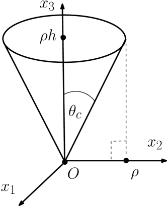
Figure 1. Schematic of a circular flight path.

Hence if there is an artifact for the circular trajectory case, that artifact must have $R\neq R^{\prime}$. (As it turns out, neither are they at points that are inverted with respect to the circle.) This is in contrast to standard monostatic SAR, since in that case $R=R^{\prime}$.

Remark 3.

The above shows that any artifacts arising from Doppler imaging for a circular flight path must appear in a location which is different from their location in standard monostatic SAR for the same flight path. Therefore, in principle, it might be possible to combine traditional monostatic SAR with Doppler SAR imaging in order to identify and remove artifacts.

In the next subsection, we investigate if it is possible to localize any backprojected artifacts to be outside the region of interest (ROI).

7.2. Condition for $\mathcal{C}$ to be a local canonical graph

From the discussion in §3.1, we know that if $\mathcal{C}$ satisfies the Bolker condition (21) then backprojection results in an artifact-free image. We initially consider the first part of the Bolker condition, namely the requirement that $\mathcal{C}$ is a local canonical graph, and need to determine where the derivative of the left projection $\pi_{L}$ has full rank, i.e., $\hbox{rank}(D\pi_{L})=4$. We may parametrize $\mathcal{C}$ using coordinates $(s,\tau,\mathbf{x})$, with respect to which

(40) $$\pi_{L}(s,\tau,\mathbf{x})=(s,\omega_{0}(1-2\dot{R}/c_{0}),2\omega_{0}\tau\ddot{R}/c_{0},\tau)\ .$$

Next, to make the study of $\pi_{L}$ easier, introduce a new, $s$-dependent coordinate system in the plane, $(u,v)$, defined by

(41) $$\mathbf{x}-\rho\mathbf{e}=\rho hS\mathbf{e}+\rho h\frac{u}{\sqrt{1-u^{2}}}C\mathbf{e}^{\perp},$$

where

$$S=S(v)=\sinh(v),$$

(42) $$C=C(v)=\cosh(v).$$

Note that for $s,\,\mathbf{x}$ ranging over compact sets, $u$ satisfies $|u|\leq 1-\epsilon$ for some $\epsilon>0$, and thus $1-u^{2}$ is bounded away from 0. The $(u,v)$ coordinates are closely related to elliptic cylindrical coordinates, but in the plane and centered directly below the antenna; cf. [3, §2.7].

Figure 2. The curves of constant $u$ (hyperbolas) and constant $v$ (vertical lines) for a location on the flight path in which the flight velocity vector is along the vertical axis. The coordinate system is centered directly under the antenna.

We note that since $\mathbf{e}$ is perpendicular to $\mathbf{e}^{\perp}$, we have immediately

(43) $$(\mathbf{x}-\rho\mathbf{e})\cdot\mathbf{e}=\rho hS.$$

The new coordinate system is better understood once we have calculated $\dot{R}$ in the new coordinates, as follows. From (36) and (41) we have

(44) $$\dot{R}=-\rho^{2}\frac{huC}{R\sqrt{1-u^{2}}},$$

where

$$R^{2}=\rho^{2}h^{2}S^{2}+\frac{\rho^{2}h^{2}u^{2}C^{2}}{1-u^{2}}+\rho^{2}h^{2},$$

so that

(45) $$R =\rho h\sqrt{(1+S^{2})+\frac{u^{2}C^{2}}{1-u^{2}}}=\rho h\sqrt{\frac{(1-u^{2})C^{2}+u^{2}C^{2}}{1-u^{2}}}=\frac{\rho hC}{\sqrt{1-u^{2}}},$$

where we have used $C^{2}-S^{2}=1$. Hence, comparing (45) with (44), we find

(46) $$\dot{R}=-\rho u.$$

Thus the coordinate $u$ is simply proportional to the Doppler shift. Because $\dot{\bm{{\gamma}}}=(\rho\mathbf{e}^{\perp},0)$, from comparing (46) with (36), we see that $u=\widehat{\mathbf{R}}\cdot(\mathbf{e}^{\perp},0)$, which is clearly bounded in magnitude by $1$. The set $u=\pm 1$ corresponds to the line on the ground directly under the tangent to the flight path at $\mathbf{e}(s)$, and we exclude this by keeping the antenna beam pattern away from the direction of travel (forward and backward).

Observe that we may also parametrize $\mathcal{C}$ with the coordinates $(s,\tau,u,v)$. To see this, one needs to check that

(47) $$\left|\frac{\partial(x_{1},x_{2})}{\partial(u,v)}\right|=\rho^{2}\bigg{|}\begin{pmatrix}a\mathbf{e}^{\perp}\,,&(b\mathbf{e}+d\mathbf{e}^{\perp})\end{pmatrix}\bigg{|}\neq 0,$$

where

(48) $$a:=hC(v)\frac{1}{(1-u^{2})^{3/2}};\quad b:=hC(v);\quad d:=hS(v)\frac{u}{\sqrt{1-u^{2}}}.$$

(47) clearly holds true since $h>0$ means that both $a$ and $b$ in (48) are nonzero.

Therefore, by avoiding data from the forward and backward directions (or, alternatively, filtering out echoes associated to values of $\dot{R}$ near $\pm\rho$), we have that $(s,\tau,u,v)$ forms a valid coordinate system on $\mathcal{C}$. The coordinate system $(s,\tau,u,v)$ is designed to make any degeneracy of the projection $\pi_{L}$ appear in a single variable, namely $v$. In fact, in terms of $(s,\tau,u,v)$, one has

(49) $$\pi_{L}(s,\tau,u,v)=(s,\omega_{0}(1+2u\rho/c_{0}),2\omega_{0}\tau\ddot{R}(u,v)/c_{0},\tau),$$

To classify the singularities of $\pi_{L}$, one needs to find first the set where $D\pi_{L}$ drops rank, i.e, where

$$\frac{\partial\ddot{R}}{\partial v}=0\ .$$

Computing $\ddot{R}$ in the original coordinates $x_{1},x_{2}$ first, and then rewriting it in the new coordinates $u,v$ using (29) and (30) one obtains

$$\ddot{R} = \rho\frac{\mathbf{x}\cdot\mathbf{e}}{R}-\rho^{2}\frac{(\mathbf{x}\cdot\mathbf{e}^{\perp})^{2}}{R^{3}}$$

$$= \rho(1+hS)\frac{\sqrt{1-u^{2}}}{hC}-\rho\frac{h^{2}u^{2}C^{2}}{1-u^{2}}\cdot\frac{(1-u^{2})^{3/2}}{h^{3}C^{3}},$$

which leads to

(50) $$\ddot{R}=\rho\frac{\sqrt{1-u^{2}}}{h}\left(\frac{1+hS-u^{2}}{C}\right)\ .$$

Therefore, setting the $v$-derivative of (50) equal to zero shows that the set $\Sigma$ of points where $\pi_{L}$ drops rank is given by

(51) $$\Sigma=\left\{\,(s,\tau,u,v)\in\mathcal{C}:\,f(u,v):=h^{2}+(u^{2}-1)Sh=0\,\right\}.$$

Remark 4.

In $(u,v)$ coordinates, $\bf x=\bf 0$ corresponds to $(u_{0},v_{0})=(0,\sinh^{-1}(-1/h))$, where we have used (41). Since $f(u_{0},v_{0})=h^{2}+1>0$, we see that the fiber of $\Sigma$ lying over $\bf x=\bf 0$ is empty.

In particular, $D\pi_{L}$ is of full rank if and only if $f\neq 0$, where $f$ is defined as in (51). Since $Sh=\frac{(\mathbf{x}-\rho\mathbf{e})\cdot\mathbf{e}}{\rho}$, we have $f>0$ iff

$$(1-u^{2})(\mathbf{x}-\rho\mathbf{e})\cdot\mathbf{e}<\rho h^{2}.$$

A sufficient condition for this is

(52) $$(\mathbf{x}-\rho\mathbf{e})\cdot\mathbf{e}<\rho h^{2},$$

and a sufficient, $\mathbf{e}$-independent condition for this to hold is that

$$\mathbf{x}\in\mathcal{D}_{h,\rho}:=\left\{\ \mathbf{x}\in\mathbb{R}^{2}\ :\ |\mathbf{x}|<\rho(h^{2}+1)\right\}.$$

Summarizing our analysis so far: Suppose that $\Sigma$ is not in the microlocal support of $\mathcal{F}$ (for example, suppose that beam forming ensures that only points in $\mathcal{D}_{h,\rho}$ are illuminated). Then the canonical relation of $\mathcal{F}$ is a local canonical graph.

Remark 5.

If the flight path only consists of a portion of the full circle, then equation (56) below could be used to enlarge the region $\mathcal{D}_{h,\rho}$ where the canonical relation of $\mathcal{F}$ is a local canonical graph. We do not pursue this idea further here.

Instead, in the next three subsections we analyze the structure of $\mathcal{C}$ near $\Sigma$. It will be convenient to introduce another set of coordinates as follows:

(53) $$p:=(\mathbf{x}-\rho\mathbf{e})\cdot\mathbf{e}/\rho=hS,$$

(54) $$q:=(\mathbf{x}-\rho\mathbf{e})\cdot\mathbf{e}^{\perp}/\rho=\mathbf{x}\cdot\mathbf{e}^{\perp}/\rho.$$

Observe that $(s,\tau,p,q)$ also form a coordinate system on the canonical relation $\mathcal{C}$. Indeed, since we have already remarked that $(s,\tau,x_{1},x_{2})$ are coordinates on $\mathcal{C}$, one only has to notice that for a fixed $(s,\tau)$-value, the map $(x_{1},x_{2})\mapsto(p,q)$ is a diffeomorphism since the vectors $d_{\mathbf{x}}p=\mathbf{e}/\rho$ and $d_{\mathbf{x}}q=\mathbf{e}^{\perp}/\rho$ are linearly independent. Points on $\Sigma$ satisfy

$$h^{2}+(u^{2}-1)Sh=0,$$

which from (45) leads to

$$h^{2}-\frac{\rho^{2}h^{2}C^{2}}{R^{2}}p=0,$$

which, with $C^{2}-S^{2}=1$, leads to

$$h^{2}R^{2}-\rho^{2}(h^{2}+h^{2}S^{2})p=0,$$

and hence

(55) $$h^{2}R^{2}-\rho^{2}(h^{2}+p^{2})p=0.$$

Therefore

(56) $$g(s,x):=h^{2}R^{2}(s,x)-\rho^{2}(h^{2}+p^{2}(s,x))p(s,x)=0\$$

is a defining equation for $\Sigma$. Since $R^{2}=\rho^{2}(p^{2}+q^{2}+h^{2})$, (56) can also be re-written as

$$h^{2}\rho^{2}(h^{2}+p^{2}+q^{2})-\rho^{2}(h^{2}+p^{2})p=0.$$

Hence

(57) $$\tilde{g}(p,q):=p^{3}-h^{2}(p^{2}+q^{2})+h^{2}p-h^{4}=0$$

is also a defining equation for $\Sigma$. We will next make use of $\tilde{g}$ to analyze the properties of $\Sigma$.

Proof of Theorem 3. Due to the length of the proof, it will be presented in parts: first we consider the singularity of $\pi_{L}$ (Sec. 7.3), then the singularity of $\pi_{R}$ (Sec. 7.4) and finally the elimination of artifacts (Sec. 7.5).

7.3. The singularity of $\pi_{L}$

We showed in the last section that $D\pi_{L}$ drops rank at $\Sigma$. The following lemma establishes a key property of $\Sigma$.

Lemma 1.

The function $\tilde{g}$ in (57) is a defining function for $\Sigma$: $d\tilde{g}\neq 0$ at all points of $\Sigma$.

Proof.

Clearly $(\partial\tilde{g}/\partial q)(p,q)\neq 0$ when $q\neq 0$, so we just need to check $(\partial\tilde{g}/\partial p)(p,0)\neq 0$ whenever $\tilde{g}(p,0)=0$. To see this, we argue as follows: note that

$$\frac{\partial\tilde{g}}{\partial p}(p,q)=3p^{2}-2h^{2}p+h^{2}.$$

Recall that $p=hS$ and suppose for contradiction that $(\partial\tilde{g}/\partial p)(p,0)=\tilde{g}(p,0)=0$ for some $p$. Then

$$\frac{\partial\tilde{g}}{\partial p}(p,0)=0\Rightarrow 3(hS)^{2}-2h^{2}(hS)+h^{2}=0$$

(58) $$\Rightarrow 3S^{2}-2hS+1=0$$

and

$$\tilde{g}(p,0)=0\Rightarrow(hS)^{3}-h^{2}(hS)^{2}+h^{3}S-h^{4}=0$$

(59) $$\Rightarrow hS^{3}-h^{2}S^{2}+hS-h^{2}=0.$$

Subsitituting (58) into (59) gives

$$hS^{3}-h^{2}S^{2}+hS+3h^{2}S^{2}-2h^{3}S=0$$

$$\Rightarrow S^{2}+2hS+(1-2h^{2})=0,$$

where we have cancelled a factor of $hS$, which is valid since (58) tells us that $S\neq 0$. The roots of this quadratic equation are

(60) $$S=-h\pm\sqrt{3h^{2}-1}.$$

Recalling that for points in $\Sigma$ we have

$$(1-u^{2})S=h$$

and substituting this into (60) gives

(61) $$(1-u^{2})(-h\pm\sqrt{3h^{2}-1})=h,$$

which can only be true if we take the plus sign (since $0<h,0<1-u^{2}$). Simplifying (61), we get

$$\sqrt{3h^{2}-1}=h+\frac{h}{1-u^{2}},$$

hence

$$h^{2}\left\{3-\left(\frac{2-u^{2}}{1-u^{2}}\right)^{2}\right\}=1,$$

which leads to

$$\frac{3(1-u^{2})^{2}-(1+(1-u^{2}))^{2}-1}{(1-u^{2})^{2}}=1,$$

(62) $$\frac{2(1-u^{2})(-u^{2})-1}{(1-u^{2})^{2}}=1.$$

This leads to a contradiction since the left-hand side of (62) is strictly negative and it completes the proof of the Lemma. ∎

Note that Lemma 1 shows that $\Sigma$ is a smooth hypersurface in $\mathcal{C}$.

If we illuminate a neighborhood of the boundary $\partial\mathcal{D}_{h,\rho}$, then it is of interest to know what kind of singularity $\pi_{L}$ has at $\Sigma$. This is answered by the next lemma.

Lemma 2.

The projection $\pi_{L}$ has a fold singularity at $\Sigma$.

Proof.

Note that, at points of $\Sigma$, $\ker(D\pi_{L})=\textnormal{span}\{\partial_{v}\}$ and we saw from the proof of Lemma 1 that $d\tilde{g}\neq 0$ there as well, so $\pi_{L}$ drops rank simply at $\Sigma$. Moreover,

$$\left.\frac{\partial f}{\partial v}\right|_{\Sigma}=-(1-u^{2})hC\neq 0.$$

It follows that $\ker(D\pi_{L})$ intersects $T\Sigma$ transversally, proving the lemma. ∎

7.4. The singularity of $\pi_{R}$

Since $D\pi_{L}$ drops rank by 1 at $\Sigma$, the Thom-Boardman notation of singularity theory suggest relabeling $\Sigma$ as $\Sigma_{1}$ [18]. Then, equality (26) shows that $\ker(D\pi_{R})$ at points of $\Sigma_{1}$, denoted $\ker(D\pi_{R}|_{\Sigma_{1}})$ is spanned by a linear combinations of $\partial_{s}$ and $\partial_{\tau}$. Since $g$ does not depend on $\tau$, it makes sense to investigate the degree to which $g$ vanishes with respect to $s$ at $\Sigma$. Noting that $\dot{p}=(\mathbf{x}\cdot\mathbf{e}^{\perp})/\rho$, we have

(63) $$g_{s} = 2h^{2}R\dot{R}-\rho(h^{2}+p^{2})(\mathbf{x}\cdot\mathbf{e}^{\perp})-2\rho p^{2}(\mathbf{x}\cdot\mathbf{e}^{\perp})$$

$$= -2\rho h^{2}(\mathbf{x}\cdot\mathbf{e}^{\perp})-\rho(h^{2}+p^{2})(\mathbf{x}\cdot\mathbf{e}^{\perp})-2\rho p^{2}(\mathbf{x}\cdot\mathbf{e}^{\perp})$$

$$= -3\rho(h^{2}+p^{2})(\mathbf{x}\cdot\mathbf{e}^{\perp})$$

Hence, if $g(s,\tau,\mathbf{x})=0$, then $g_{s}(s,\tau,\mathbf{x})=0$ iff $\mathbf{x}\cdot\mathbf{e}^{\perp}=0$, i.e., when $\mathbf{x}$ lies on the line directly to the left or right of the transceiver. Thus, again using the Thom-Boardman notation, we investigate the properties of

$$\Sigma_{1,1}:=\left\{(s,\tau,\mathbf{x})\in\Sigma_{1}\ :\mathbf{x}\cdot\mathbf{e}^{\perp}=0\ \right\}=\Big{\{}(s,\tau,p,q)\in\mathcal{C}\ :\tilde{g}(p,q)=0,q=0\ \Big{\}}$$

as follows.

Lemma 3.

$\Sigma_{1,1}$ is a smooth, codimension one, immersed submanifold of $\Sigma_{1}$.

Proof.

We saw in the proof of Lemma 1 that $\tilde{g}(p,0)=0$ implies $\frac{\partial\tilde{g}}{\partial p}(p,0)\neq 0$ and since $\tilde{g}$ is smooth, the lemma follows. ∎

Lemma 4.

The projection $\pi_{R}$ has a cusp singularity at $\Sigma_{1,1}$.

Proof.

The non-vanishing of $d\tilde{g}|_{\Sigma_{1,1}}$ means that $\pi_{R}$ drops rank by one, with $\det(D\pi_{R})$ vanishing simply at $\Sigma_{1}$. Moreover, ker$(D\pi_{R}|_{\Sigma_{1,1}})\subset T\Sigma_{1}$. The vector field $\partial_{s}|_{\Sigma_{1}}$ is tangent to $\Sigma_{1}$ at points of $\Sigma_{1,1}$, since $g$ and $g_{s}$ are defining functions for $\Sigma_{1}$ and $\Sigma_{1,1}$ resp. Suppose that $g_{ss}(s,\tau,\mathbf{x})=0$ for some point $(s,\tau,\mathbf{x})\in\Sigma_{1,1}$. Then equation (63) implies $\mathbf{x}\cdot\mathbf{e}=\mathbf{x}\cdot\mathbf{e}^{\perp}=0$, meaning that $\mathbf{x}=\mathbf{0}$. This contradicts Remark 4 since $\Sigma_{1,1}\subset\Sigma_{1}=\Sigma$. Therefore $dg(\partial_{s})$ has a simple zero at $\Sigma_{1,1}$. In $(p,q)$ coordinates, $g_{s}$ becomes $\tilde{g}_{s}=-3\rho^{2}q(p^{2}+h^{2})$. We need to check that $d\tilde{g}|_{\Sigma_{1,1}}$ and $d\tilde{g}_{s}|_{\Sigma_{1,1}}$ are linearly independent. One has

$$dg(p,0)=(\partial\tilde{g}/\partial p(p,0),0)\ ;\quad d\tilde{g}_{s}(p,0)=(0,-3\rho^{2}(h^{2}+p^{2}))$$

However, we already saw in the proof of Lemma 1 that $\partial\tilde{g}/\partial p(p,0)\neq 0$ at points of $\Sigma_{1,1}$. Therefore, $d\tilde{g}$ and $d\tilde{g}_{s}$ are linearly independent at $\Sigma_{1,1}$. It now follows (see Def. 3) that $\pi_{R}$ has a cusp singularity at $\Sigma_{1,1}$, and the lemma is proved. ∎

7.5. Criteria for absence of artifacts

In general, even if through beam forming the microlocal support of $\mathcal{F}$ is restricted to a set where $\mathcal{C}$ is a local canonical graph, if $\pi_{L}$ is not injective, i.e., if the Bolker condition (21) is violated, one can expect that the backprojected image $\mathcal{F}^{*}W$ will contain artifacts. Recalling (49), we see that the question of whether artifacts will be present in the backprojected image boils down to the whether or not, for a fixed value of $u$, the map

$$\mathcal{V}:v\mapsto\ddot{R}$$

is injective. So, using (50), suppose that we specifiy a value

$$\alpha:=\mathcal{V}(v)=\rho\frac{\sqrt{1-u^{2}}}{h}\left(\frac{1+hS-u^{2}}{C}\right)$$

Then we have that

$$h\alpha(e^{v}+e^{-v})=\rho\sqrt{1-u^{2}}\left\{2(1-u^{2})+h(e^{v}-e^{-v})\right\}$$

(64) $$\Rightarrow h\beta_{-}e^{v}-h\beta_{+}e^{-v}+2\rho(1-u^{2})^{3/2}=0,$$

where

$$\beta_{\pm}:=\rho\sqrt{1-u^{2}}\pm\alpha\ .$$

We cannot have both $\beta_{+}=0,\beta_{-}=0$, since $\rho>0,u^{2}\neq 1$. We consider both cases separately, as follows.

Case 1: Assume $\beta_{-}\neq 0$. Divide across (64) by $h\beta_{-}$ to get

(65) $$e^{v}-\left(\frac{\beta_{+}}{\beta_{-}}\right)e^{-v}+2\eta=0,$$

where

$$\eta:=\frac{\rho(1-u^{2})^{3/2}}{h\beta_{-}}.$$

Let $y:=e^{v}$ and multiply equation (65) by $y$ to get the quadratic equation

$$y^{2}+2\eta y-\beta_{+}/\beta_{-}=0.$$

The solutions of this equation are

$$y_{\pm}=-\eta\pm\sqrt{\eta^{2}+\beta_{+}/\beta_{-}}$$

(66) $$\Rightarrow y_{\pm}=-\eta\left(1\pm\sqrt{1+\beta_{+}/(\eta^{2}\beta_{-})}\ \right)$$

From the definition of $y$, we must have $y_{\pm}=e^{v_{\pm}}>0$ for some value of $v_{\pm}$ and therefore, $y_{\pm}>0$.

Next we study the term under the square root in (66):

$$\frac{\beta_{+}}{\eta^{2}\beta_{-}}=\frac{h^{2}}{\rho^{2}(1-u^{2})^{3}}\left\{\rho^{2}(1-u^{2})-\alpha^{2}\right\}\ .$$

Since $\eta$ has the same sign as $\beta_{-}$, the map $\mathcal{V}$ will be injective if

(67) $$\alpha^{2}<\rho^{2}(1-u^{2})$$

since then, $y_{+}$ is the only possible positive root if $\beta_{-}<0$, while $y_{-}$ is the only possible root if $\beta_{-}>0$.

Case 2: Assume $\beta_{+}\neq 0$. Dividing (64) across by $h\beta_{+}$ we obtain

(68) $$e^{-v}-\left(\frac{\beta_{-}}{\beta_{+}}\right)e^{v}-2\tilde{\eta}=0,$$

where

$$\tilde{\eta}=\frac{\rho(1-u^{2})^{3/2}}{h\beta_{+}}.$$

Letting $\tilde{y}:=e^{-v}$ and multiplying (68) across by $\tilde{y}$ we get

$$\tilde{y}^{2}-2\tilde{\eta}\tilde{y}-\frac{\beta_{-}}{\beta_{+}}=0.$$

This quadratic equation has solutions

$$\tilde{y}_{\pm}=\tilde{\eta}\pm\sqrt{\tilde{\eta}^{2}+\beta_{-}/\beta_{+}}$$

$$\Rightarrow\tilde{y}_{\pm}=\tilde{\eta}\left(1\pm\sqrt{1+(\beta_{-}/(\tilde{\eta}^{2}\beta_{+})}\ \right).$$

One can easily check that condition (67) also guarantees that $\beta_{-}/({\tilde{\eta}^{2}\beta_{+})}>0$, which establishes injectivity of $\mathcal{V}$ in this case too.

Lemma 5.

The following inequality guarantees injectivity of $\mathcal{V}$:

(69) $$(\mathbf{x}-\rho\mathbf{e})\cdot\mathbf{e}<\rho\left(\frac{h^{2}-1}{2}\right)\ .$$

Proof.

In fact, if (69) holds, then from (43) we have

(70) $$hS<\frac{h^{2}-1}{2}\ .$$

Since $0\leq u^{2}\leq 1$, this implies the inequality $1-u^{2}+2hS<h^{2}$; the left of which is decreased by multiplying by $1-u^{2}$ to obtain $(1-u^{2})(1-u^{2}+2hS)<h^{2}=h^{2}(C^{2}-S^{2})$. Moving $h^{2}S^{2}$ to the left side, we obtain $(1-u^{2}+hS)^{2}<h^{2}C^{2}$, which can be rewritten as $\frac{\rho^{2}(1-u^{2})}{h^{2}}\left(\frac{1-u^{2}+hS}{C}\right)^{2}<\rho^{2}(1-u^{2})$. This is exactly condition (67), as claimed, so that (69) is sufficient for injectivity of $\mathcal{V}$. ∎

Writing (69) as $\mathbf{x}\cdot\mathbf{e}<\rho+\rho(h^{2}-1)/2$ and considering all possible locations on the flight path, it then follows that a sufficient condition to guarantee injectivity of $\mathcal{V}$ is

(71) $$|\mathbf{x}|<\rho\left(\frac{h^{2}+1}{2}\right)\quad\Leftrightarrow\quad\mathbf{x}\in\mathcal{D}_{h,\rho/2}\ .$$

This concludes the proof of Theorem 3.∎

Remark 6.

Note that condition (71) implies that the left projection $\pi_{L}$ is injective, and also guarantees that condition (52) is automatically satisfied, so that $\pi_{L}$ is an immersion. Therefore, $\mathcal{C}$ is a canonical graph over the region defined by (71), ensuring artifact-free imaging of scenes there via filtered backprojection.

Remark 7.

To summarize the microlocal analysis so far of DSAR for a circular flight path, $\mathcal{C}$ is a canonical relation whose projections, $\pi_{L}$ and $\pi_{R}$, are of fold and cusp type, resp. A similar geometry appeared in [16] in the case of monostatic SAR when the flight path had simple inflection points. In that situation it was shown that $\mathcal{F}^{*}\mathcal{F}$ produces an artifact relation which is a canonical relation, with a codimension-two set of points where it is nonsmooth, called an open umbrella; see [15] for background material on umbrellas and their relevance in seismic imaging, and [16] for how this geometry arises in monostatic SAR.

8. First order correction to the start-stop approximation

We now describe and analyze a correction to the start-stop approximation, Assumption 3, which in the form of $R(t+T_{tot})=R(t)$ was substituted into (4) and used to derive (2) and thus (10). The correction we now consider comes from modifying the discussion below (3) by including a first order term in the expansion of $R(t+T_{tot})$. See also [39, 7] for discussions of the start-stop approximation and its limitations.

As in Sec. 2, $T_{tot}$ is determined implicitly by (4), namely $c_{0}T_{tot}=R(t)+R\left(t+T_{tot}\right)$. However, we now expand

$$c_{0}T_{tot}=R(t)+R\left(t+T_{tot}\right)\approx 2R(t)+\dot{R}(t)\cdot T_{tot}$$

Solving for $T_{tot}$ and ignoring terms $\mathcal{O}(c_{0}^{-3})$, we obtain the first order refinement of the start-stop approximation, namely that the total travel time is

(72) $$T_{tot}\approx 2c_{0}^{-1}R(t)+2c_{0}^{-2}R(t)\dot{R}(t)$$

and thus, under this refined approximation, the scattered wave arrives at time

$$t_{sc}=t+2c_{0}^{-1}R(t)+2c_{0}^{-2}R(t)\dot{R}(t).$$

Using this, the analogue of $W_{0}$ from (2) is

$$W_{1}(s,\omega) :=\int e^{i\omega(t-s)}\ell(\omega_{0}(t-s))d(t)dt$$

(73) $$=\int e^{i\omega(t-s)}\ell(\omega_{0}(t-s))\int\frac{e^{-i\omega_{0}\left(t-2\left[c_{0}^{-1}R\left(t\right)+c_{0}^{-2}R\left(t\right)\dot{R}\left(t\right)\right]\right)}}{\left(4\pi R\left(t\right)\right)\left(4\pi R\left(t_{sc}\right)\right)}V(\mathbf{x})d\mathbf{x}dt$$

Substituting into (8) the linear terms of the Taylor expansions

(74) $$R(t)=R(s)+\dot{R}(s)(t-s)+\cdots,\quad\dot{R}(t)=\dot{R}(s)+\ddot{R}(s)(t-s)+\cdots,$$

and, calculating modulo $(t-s)^{2}$, yields the approximation $W_{1}$ of $W$ analogous to (10):

(75) $$W_{1}(s,\omega)=\int e^{i\phi(s,\omega,\mathbf{x};\tau)}a(\mathbf{x},s;\tau)V(\mathbf{x})d\tau d\mathbf{x},$$

where

(76) $$\phi=\tau\left(\omega-\omega_{0}+2\omega_{0}\left[c_{0}^{-1}\dot{R}\left(s\right)+c_{0}^{-2}\left(R\left(s\right)\ddot{R}\left(s\right)+\dot{R}(s)^{2}\right)\right]\right)$$

and

(77) $$a(\mathbf{x},s;\tau)=e^{i\omega_{0}\left[2\left(c_{0}^{-1}R\left(s\right)+c_{0}^{-2}R\left(s\right)\dot{R}\left(s\right)\right)-s\right]}(4\pi)^{-2}R\left(s\right)^{-1}R\left(s_{sc}\right)^{-1}\ell(\omega_{0}\tau).$$

Rewriting the expression in (76) that multiplies $c_{0}^{-2}$ as $\left(1/2\right)\left(R^{2}\right)^{\mathbf{..}}$ for compactness (where the superscript upper right dots still denote differentiation in $t$), one sees that this modified phase function $\phi$ parametrizes the canonical relation

(78) $$\mathcal{C}_{mod}\!\!\! = \!\!\!\Big{\{}\Big{(}s,\omega_{0}-2\omega_{0}\left[c_{0}^{-1}\dot{R}+\left(1/2\right)c_{0}^{-2}\left(R^{2}\right)^{\mathbf{..}}\right],2\tau\omega_{0}\left(c_{0}^{-1}\ddot{R}+c_{0}^{-2}(1/2)(R^{2})^{\mathbf{\cdots}}\right),\tau;$$

$$\quad\,\mathbf{x},-2\tau\omega_{0}\left[c_{0}^{-1}{d}_{\mathbf{x}}\dot{R}+\left(1/2\right)c_{0}^{-2}{d}_{\mathbf{x}}\left(R^{2}\right)^{\mathbf{..}}\right]\Big{)}:s\in\mathbb{R},\mathbf{x}\in\mathbb{R}^{2},\tau\in\mathbb{R}\setminus 0\Big{\}}.$$

The fold/blowdown structure of the canonical relation in the case of the linear flight track, established in §6, is not structurally stable, since arbitrarily small perturbations of blowdowns are not (in general) blowdowns. Nevertheless, we now show that under the first order correction to the start-stop approximation, $\mathcal{C}_{mod}$ is still a fold/blowdown, indicating the robustness of our approach.

To see this, note that the analogue of (27) taking the correction into account is

(79) $$\frac{D(\bm{\xi})}{D(s,\tau)}=-2\omega_{0}\left[\tau\ddot{\Gamma},\,\dot{\Gamma}\right],$$

where

$$\Gamma(\mathbf{x},s)=c_{0}^{-1}d_{\mathbf{x}}R+(1/2)c_{0}^{-2}\dot{d}_{\mathbf{x}}(R^{2})=c_{0}^{-1}d_{\mathbf{x}}R+c_{0}^{-2}\left[\dot{R}d_{\mathbf{x}}R+Rd_{\mathbf{x}}\dot{R}\right].$$

(Thus, $\mathcal{C}_{mod}$ is nondegenerate at a point if and only if $\Gamma$ is a smooth curve with nonzero curvature for the corresponding $\mathbf{x},s$.) One computes

(80) $$\dot{\Gamma}=c_{0}^{-1}d_{\mathbf{x}}\dot{R}+c_{0}^{-2}\left[\ddot{R}d_{\mathbf{x}}R+{2}\dot{R}d_{\mathbf{x}}\dot{R}+Rd_{\mathbf{x}}\ddot{R}\right]$$

and

(81) $$\ddot{\Gamma}=c_{0}^{-1}d_{\mathbf{x}}\ddot{R}+c_{0}^{-2}\left[\dddot{R}d_{\mathbf{x}}R+{3}\ddot{R}d_{\mathbf{x}}\dot{R}+{3}\dot{R}d_{\mathbf{x}}\ddot{R}+Rd_{\mathbf{x}}\dddot{R}\right]$$

Using (30-34), one finds

$$\ddot{R}d_{\mathbf{x}}R+{2}\dot{R}d_{\mathbf{x}}\dot{R}+Rd_{\mathbf{x}}\ddot{R}=\ 0\hbox{ and }\dddot{R}d_{\mathbf{x}}R+{3}\ddot{R}d_{\mathbf{x}}\dot{R}+{3}\dot{R}d_{\mathbf{x}}\ddot{R}+Rd_{\mathbf{x}}\dddot{R}=0.$$

Thus

(82) $$\dot{\Gamma}=(c_{0}^{-1}R^{-3})\left[-\left(x_{2}^{2}+h^{2}\right),\left(x_{1}-s\right)x_{2}\right].$$

Differentiating this directly yields

$$\ddot{\Gamma}=c_{0}^{-1}R^{-5}\big{(}-3(x_{1}-s)(x_{2}^{2}+h^{2}),\ 2x_{2}R^{2}-3x_{2}(x_{2}^{2}+h^{2})\big{)},$$

so that

$$\det\left[\ddot{\Gamma},\dot{\Gamma}\right]=\left(\frac{1}{c_{0}^{2}R^{6}}\right)x_{2}(x_{2}^{2}+h^{2}),$$

which vanishes to first order at $(s,\mathbf{x},\tau)\in\Sigma=\{x_{2}=0\}$. Furthermore, at these points, ker$(D\pi_{R})=\mathbb{R}\cdot\frac{\partial}{\partial s}\subset T\Sigma$, so that $\pi_{R}$ has a blowdown singularity at $\Sigma$. A similar calculation shows that $D\pi_{L}$ has a kernel whose nonzero elements have a nonzero coefficient of $\frac{\partial}{\partial x_{2}}$, so that $\pi_{L}$ has a fold singularity at $\Sigma$, and $\mathcal{C}_{mod}$ is a fold/blowdown canonical relation.

In the case of the circular flight track, the fold/cusp structure of the canonical relation derived in §7 under the start-stop approximation, is structurally stable in the following sense: a small perturbation of the phase function (say in the $C^{4}$ topology) will result in a small perturbation of $\mathcal{C}$ and this causes small $C^{3}$ perturbations of the projections $\pi_{L}$ and $\pi_{R}$. Folds are stable under $C^{2}$ perturbations and cusps are stable under $C^{3}$ perturbations [18], and thus one expects that the first order correction to the start-stop approximation will not essentially change the microlocal analysis for a circular flight path: $\mathcal{C}_{mod}$ will still be a fold/cusp, so that the artifacts are of the same type and strength as shown above, although with their locations moved slightly. However, we have not proven this and it is a subject for future research.

9. Concluding Remarks

We briefly compare our results for Doppler SAR with the case of monostatic SAR treated in [32]. In all cases, we can expect the strength of any associated artifacts in the image to be as strong as the bona-fide part.

For the case of a linear flight path, the results for Doppler are the same as for monostatic SAR, in the sense that $\pi_{L}$ and $\pi_{R}$ have fold and blowdown singularities, resp. The normal operator $\mathcal{F}^{*}\mathcal{F}$ formed without beam forming will have the same strong artifact, i.e., $\mathcal{F}^{*}\mathcal{F}\in I^{-1,0}(\Delta,C_{\chi})$, with $C_{\chi}$ a canonical graph (cf. Remark 2 in Sec. 6).

On the other hand, for a circular flight path, the microlocal geometry for Doppler SAR differs from that for monostatic SAR: we have shown that in the case of Doppler, the singularities of $\pi_{L}$, $\pi_{R}$, are of fold and cusp type, resp., whereas for monstatic SAR, both singularities are folds [32]. Regarding the operator $\mathcal{F}^{*}\mathcal{F}$, it was shown in [11] that in the monostatic SAR, $\mathcal{F}^{*}\mathcal{F}\in I^{-1,0}(\Delta,\tilde{C})$, where $\tilde{C}$ is a two-sided fold. For Doppler SAR we expect, based on the results of Felea and Nolan [16], that $\mathcal{F}^{*}\mathcal{F}\in I^{-1}(\Delta,\tilde{C})$, where $\tilde{C}$ is an open umbrella (see Remark 7). For the circular flight path, we have described an explicit region $D_{h,\rho}$ where the wave front relation of $F$ is a canonical graph, so that no artifacts appear at the back projection, allowing accurate imaging of the terrain. In addition, as described at the end of Sec. 7.1, the artifacts arising from Doppler imaging in a circular flight path geometry are spatially separated from their location for monostatic SAR for the same flight path. It should therefore be possible to identify and remove artifacts by combining monostatic SAR data with Doppler SAR data; we hope to return to this in the future.

References

- [1] G. Ambartsoumian, R. Felea, V. Krishnan, C. Nolan and E.T. Quinto, A class of singular Fourier integral operators in synthetic aperture radar imaging, Jour. Func. Analysis 264 (2013), no. 1, 246–269.
- [2] G. Ambartsoumian, R. Felea, V. Krishnan, C. Nolan and E.T. Quinto, A class of singular FIOs in SAR imaging II: transmitter and receiver with different speeds, SIAM J. Math. Analysis 50 (2018), no. 1, 591–621.
- [3] G. Arfken, Mathematical Methods for Physicists, 2nd ed., Academic Pr., 1970.
- [4] V. Arnold, S. Gusein-Zade and A. Varchenko, Singularities of Differentiable Maps, I, Birkhäuser, Basel,1985.
- [5] B. Borden and M. Cheney, Synthetic-aperture imaging from high-Doppler-resolution measurements, Inverse Problems 21 (2005), 1–11.
- [6] T. Bröcker and L. Lander, Differentiable Germs and Catastrophes, London Math. Soc. Lect. Note Series 17, Cambridge Univ. Press, London, 1975.
- [7] M. Cheney and B. Borden, Theory of waveform-diverse moving-target spotlight synthetic-aperture radar, SIAM J. Imaging Sci. 4 (2011), no. 4, 1180–1199.
- [8] M. Cheney and B. Borden, Fundamentals of Radar Imaging, SIAM, Philadelphia, 2009.
- [9] S. Coetzee, C. Baker and H. Griffiths, Narrow band high resolution radar imaging, in Proc. 2006 IEEE Radar Conf., (April 2006), 622–625.
- [10] J. Duistermaat, Fourier integral operators, Prog. in Math. 130. Birkhäuser Boston, 1996.
- [11] R. Felea, Composition of Fourier integral operators with fold and blowdown singularities, Comm. Partial Differential Equations 30 (2005), no. 10-12, 1717–1740.
- [12] R. Felea, Composition of Fourier Integral Operators with Fold and Blow-Down Singularities, Ph.D. thesis, University of Rochester, 2004.
- [13] R. Felea, Displacement of artefacts in inverse scattering, Inverse Problems 23 (2007), no. 4, 1519.
- [14] R. Felea, R. Gaburro and C. Nolan, Microlocal analysis of SAR imaging of a dynamic reflectivity function, SIAM J. Math. Analysis 45 (2013), no. 5, 2767–2789.
- [15] R. Felea and A. Greenleaf, Fourier integral operators with open umbrellas and seismic inversion for cusp caustics, Math. Res. Lett. 17 (2010), no. 5, 867–886.
- [16] R. Felea and C. Nolan, Monostatic SAR with fold/cusp singularities, Jour. Fourier Analysis Appl. 21 (2015), no. 4, 799–821.
- [17] R. Felea and E.T. Quinto, The microlocal properties of the local 3-D SPECT operator, SIAM J. Math. Anal. 43 (2011), no. 3, 1145–1157.
- [18] M. Golubitsky and V. Guillemin, Stable mappings and their singularities, Graduate Texts in Mathematics 14, Springer-Verlag, New York-Heidelberg, 1973.
- [19] A. Greenleaf and G. Uhlmann, Nonlocal inversion formulas for the X-ray transform, Duke Math. Jour. 58 (1989), 205–240.
- [20] V. Guillemin, On some results of Gel’fand in integral geometry, in Pseudodifferential operators and applications (Notre Dame, Ind., 1984), Proc. Sympos. Pure Math., 43, Amer. Math. Soc., Providence, RI, 1985, 149–155.
- [21] V. Guillemin, Cosmology in (2+1)-dimensions, cyclic models, and deformations of . Annals of Math. Studies, 121. Princeton Univ. Press, Princeton, NJ, 1989.
- [22] V. Guillemin and G. Uhlmann, Oscillatory integrals with singular symbols, Duke Math. Jour. 48 (1981), 251–267.
- [23] L. Hörmander, Fourier integral operators, I, Acta Math. 127 (1971), no. 1-2, 79–183.
- [24] L. Hörmander, The Analysis of Linear Partial Differential Operators, III, Springer-Verlag, New York, 1985.
- [25] L. Hörmander, The Analysis of Linear Partial Differential Operators, IV, Springer-Verlag, New York, 1985.
- [26] R. Melrose and G. Uhlmann, Lagrangian intersection and the Cauchy problem, Comm. Pure Appl. Math. 32 (1979), 483–519.
- [27] D. Mensa, High Resolution Radar Imaging, Artech House, Dedham, MA, 1981.
- [28] D. Mensa, S. Halevy and G. Wade, Coherent doppler tomography for microwave imaging, Proceedings of the IEEE 71 (Feb. 1983), 254–261.
- [29] D. Mensa and G. Heidbreder, Bistatic synthetic-aperture radar imaging of rotating objects, IEEE Trans. Aerosp. and Electronic Sys. 18 (July 1982),423–431.
- [30] C.J. Nolan and W.W. Symes, Global Solution of a Linearized Inverse Problem for the Wave Equation, Comm. Partial Differential Equations 22 (1997), nos. 5-6, 919–952.
- [31] C. Nolan and M. Cheney, Synthetic aperture inversion, Inverse Problems 18 (2002), no. 1, 221–235.
- [32] C. Nolan and M. Cheney, Microlocal analysis of synthetic aperture radar, Jour. Fourier Analysis and Appl. 10 (2004), no. 2, 133–148.
- [33] E.T. Quinto and H. Rullgård, Local singularity reconstruction from integrals over curves in , Inverse Probl. Imaging 7 (2013), no. 2, 585–609.
- [34] B. Rigling, Intrinsic processing gains in noise radar, IEEE Conference on Waveform Diversity & Design Conference (2006).
- [35] M. S. Roulston and D.O. Muhleman, Synthesizing radar maps of polar regions with a doppler-only method, Applied Optics 36 (June 1997), 3912–3919.
- [36] P. Stefanov and G. Uhlmann, Is a curved flight path in SAR better than a straight one?, SIAM J. Appl. Math. 73 (2013), 1596–1612.
- [37] H. Sun, H. Feng and Y. Lu, High resolution radar tomographic imaging using single-tone cw signals, in Proc. of 2010 IEEE Radar Conference (May 2010), 975–980.
- [38] J.H. Thomson and J.E.B. Ponsonby, Two-dimensional aperture synthesis in lunar radar astronomy, Proc. R. Soc. London Ser. A 303 (1968), 477–491.
- [39] S. Tsynkov, On the use of start-stop approximation for space borne imaging, SIAM J. Imaging Sci. 2 (2009), 646–669.
- [40] L. Wang and B. Yazici, Bistatic synthetic aperture radar imaging using ultranarrowband continuous waveforms, IEEE Trans. Image Process. 21 (2012), no. 8, 3673–3686.
- [41] L. Wang and B. Yazici, Bistatic Synthetic Aperture Radar Imaging of Moving Targets Using Ultra-Narrowband Continuous Waveform, SIAM J. Imaging Sci. 7 (2014), no. 2, 824–866.
- [42] M.C. Wicks, B. Himed, J.L.E. Bracken, H. Bascom and J. Clancy, Ultra narrow band adaptive tomographic radar, in Proc. of IEEE Intern. Workshop on Comp. Adv. in Multi-sensor Adaptive Processing (Dec. 2005), 36–39.
- [43] C.E. Yarman, L. Wang and B. Yazici, Doppler synthetic aperture hitchhiker imaging, Inverse Problems 26 (2010), 065006.
- [44] B. Yazici, I.-Y. Son and H.C. Yanik, Doppler synthetic aperture radar interferometry: a novel SAR interferometry for height mapping using ultra-narrowband waveforms, Inverse Problems 34 (2018), no. 5, 055003.