2018 150 30 May

p–p, p$\mbox{--}\Lambda$ and $\Lambda\mbox{--}\Lambda$ correlations studied via femtoscopy in pp at $\sqrt{s}=7$ TeV

ALICE Collaboration ALICE Collaboration

We report on the first femtoscopic measurement of baryon pairs, such as p–p , p–$\Lambda$ and $\Lambda$–$\Lambda$ , measured by ALICE at the Large Hadron Collider (LHC) in proton-proton collisions at $\sqrt{s}=7$ TeV. This study demonstrates the feasibility of such measurements in $\mathrm{p\kern-0.50003ptp}$ collisions at ultrarelativistic energies. The femtoscopy method is employed to constrain the hyperon–nucleon and hyperon–hyperon interactions, which are still rather poorly understood. A new method to evaluate the influence of residual correlations induced by the decays of resonances and experimental impurities is hereby presented. The p–p , p–$\Lambda$ and $\Lambda$–$\Lambda$ correlation functions were fitted simultaneously with the help of a new tool developed specifically for the femtoscopy analysis in small colliding systems “Correlation Analysis Tool using the Schrödinger Equation” (CATS). Within the assumption that in $\mathrm{p\kern-0.50003ptp}$ collisions the three particle pairs originate from a common source, its radius is found to be equal to $r_{0}=1.125\pm 0.018\,\mathrm{(stat)}\,^{+0.058}_{-0.035}\,\mathrm{(syst)}$ fm. The sensitivity of the measured p–$\Lambda$ correlation is tested against different scattering parameters which are defined by the interaction among the two particles, but the statistics is not sufficient yet to discriminate among different models. The measurement of the $\Lambda$–$\Lambda$ correlation function constrains the phase space spanned by the effective range and scattering length of the strong interaction. Discrepancies between the measured scattering parameters and the resulting correlation functions at LHC and RHIC energies are discussed in the context of various models.

1 Introduction

Traditionally femtoscopy is used in heavy-ion collisions at ultrarelativistic energies to investigate the spatial-temporal evolution of the particle emitting source created during the collision [1, 2]. Assuming that the interaction for the employed particles is known, a detailed study of the geometrical extension of the emission region becomes possible [3, 4, 5, 6, 7, 8, 9, 10].
If one considers smaller colliding systems such as proton-proton ($\mathrm{p\kern-0.50003ptp}$) at TeV energies and assumes that the particle emitting source does not show a strong time dependence, one can reverse the paradigm and exploit femtoscopy to study the final state interaction (FSI). This is especially interesting in the case where the interaction strength is not well known as for hyperon–nucleon (Y–N) and hyperon–hyperon (Y–Y) pairs [11, 12, 13, 14, 15, 16, 17, 18, 19].
Hyperon–nucleon and hyperon–hyperon interactions are still rather poorly experimentally constrained and a detailed knowledge of these interactions is necessary to understand quantitatively the strangeness sector in the low-energy regime of Quantum-Chromodynamics (QCD) [20].
Hyperon–nucleon (p–$\Lambda$ and p$\mbox{--}\Sigma$) scattering experiments have been carried out in the sixties [21, 22, 23] and the measured cross sections have been used to extract scattering lengths and effective ranges for the strong nuclear potential by means of effective models such as the Extended-Soft-Core (ESC08) baryon–baryon model [24] or by means of chiral effective field theory ($\chi$EFT) approaches at leading order (LO) [25] and next-to-leading order (NLO) [26]. The results obtained from the above-mentioned models are rather different, but all confirm the attractiveness of the $\Lambda$ –nucleon ($\Lambda$–N) interaction for low hyperon momenta. In contrast to the LO results, the NLO solution claims the presence of a negative phase shift in the p–$\Lambda$ spin singlet channel for $\Lambda$ momenta larger than $p_{\Lambda}>600$ MeV/$c$. This translates into a repulsive core for the strong interaction evident at small relative distances. The same repulsive interaction is obtained in the p-wave channel within the ESC08 model [24].
The existence of hypernuclei [27] confirms that the N–$\Lambda$ is attractive within nuclear matter for densities below nuclear saturation $\rho_{0}=\,0.16~{}\mathrm{fm}^{-3}$. An average value of $U(\rho=\rho_{0},k=0)\approx\,-30$ MeV [27], with $k$ the hyperon momentum in the laboratory reference system, is extracted from hypernuclear data on the basis of a dispersion relation for hyperons in a baryonic medium at $\rho_{0}$ .
The situation for the $\Sigma$ hyperon is currently rather unclear. There are some experimental indications for the formation of $\Sigma$–hypernuclei [28, 29] but different theoretical approaches predict both attractive and repulsive interactions depending on the isospin state and partial wave [30, 24, 26]. The scarce experimental data for this hypernucleus prevents any validation of the models.
A $\Xi$–hypernucleus candidate was detected [31] and ongoing measurements suggest that the N–$\Xi$ inter-action is weakly attractive [32]. A recent work by the Lattice HAL-QCD Collaboration [33] shows how this attractive interaction could be visible in the p–$\Xi$ femtoscopy analysis, in particular by comparing correlation functions for different static source sizes. This further motivates the extension of the femtoscopic studies from heavy ions to $\mathrm{p\kern-0.50003ptp}$ collisions since in the latter case the source size decreases by about a factor of three at the LHC energies leading to an increase in the strength of the correlation signal [34].
If one considers hyperon–hyperon interactions, the most prominent example is the $\Lambda$–$\Lambda$ case. The H-dibaryon $\Lambda$–$\Lambda$ bound state was predicted [35] and later a double $\Lambda$ hypernucleus was observed  [36]. From this single measurement a shallow $\Lambda$–$\Lambda$ binding energy of few MeV was extracted, but the H-dibaryon state was never observed. Also recent lattice calculations [37] obtain a rather shallow attraction for the $\Lambda$–$\Lambda$ state.
The femtoscopy technique was employed by the STAR collaboration to study $\Lambda$–$\Lambda$ correlations in Au–Au collisions at $\sqrt{s_{\mathrm{NN}}}=200$ GeV [16]. First a shallow repulsive interaction was reported for the $\Lambda$–$\Lambda$ system, but in an alternative analysis, where the residual correlations were treated more accurately [38], a shallow attractive interaction was confirmed. These analyses demonstrate the limitations of such measurements in heavy-ion collisions, where the source parameters are time-dependent and the emission time might not be the same for all hadron species.
The need for more experimental data to study the hyperon–nucleon, hyperon–hyperon and even the hyperon–nucleon–nucleon interaction has become more crucial in recent years due to its connection to the modeling of astrophysical objects like neutron stars  [39, 40, 41, 42]. In the inner core of these objects the appearance of hyperons is a possible scenario since their creation at finite density becomes energetically favored in comparison with a purely neutron matter composition  [41]. However, the appearance of these additional degrees of freedom leads to a softening of the nuclear matter equation of state (EOS) [43] making the EOS incompatible with the observation of neutron stars as heavy as two solar masses [44, 45]. This goes under the name of the ’hyperon puzzle’. Many attempts were made to solve this puzzle, e.g. by introducing three-body forces for $\Lambda$NN leading to an additional repulsion that can counterbalance the large gravitational pressure and finally allow for larger neutron star masses [46, 47, 48, 49]. A repulsive core for the two body forces would also stiffen the EOS containing hyperons.
In order to constrain the parameter space of such models a detailed knowledge of the hyperon–nucleon, including $\Sigma$ and $\Xi$ states, and of the hyperon–nucleon–nucleon interaction is mandatory.
This work presents an alternative to scattering experiments, using the femtoscopy technique to study the Y–N and Y–Y interactions in $\mathrm{p\kern-0.50003ptp}$ collisions at $\sqrt{s}=7\,$TeV. We show that $\mathrm{p\kern-0.50003ptp}$ collisions at the LHC are extremely well suited to investigate baryon–baryon final state interactions and that the measurement of the correlation function is not contaminated with the mini-jet background visible in meson–meson correlations [50, 51]. The extracted p–p , p–$\Lambda$ and $\Lambda$–$\Lambda$ correlations have been compared to the predicted function obtained by solving the Schrödinger equation exactly by employing the Argonne $v_{18}$ potential [52] for p–p pairs and different scattering parameters available in the literature for p–$\Lambda$ and $\Lambda$–$\Lambda$ pairs. The predictions for the correlation function used to fit the data are obtained with the newly developed CATS framework [53]. A common source with a constant size is assumed and the value of the radius is extracted.
The work is organized in the following way: in Section II the experiment setup and the analysis technique are briefly introduced. In Section III the femtoscopy technique and the theoretical models employed are discussed. In Section IV the sources of systematic uncertainties are summarized and finally in Section V the results for the p–p , p–$\Lambda$ and $\Lambda$–$\Lambda$ correlation function are presented.

2 Data analysis

In this paper we present results from studies of the p–p , p–$\Lambda$ and $\Lambda$–$\Lambda$ correlations in $\mathrm{p\kern-0.50003ptp}$ collisions at $\sqrt{s}=7$ TeV employing the data collected by ALICE in 2010 during the LHC Run 1. Approximately $3.4\times 10^{8}$ minimum bias events have been used for the analysis, before event and track selection. A detailed description of the ALICE detector and its performance in the LHC Run 1 (2009-2013) is given in [54, 55]. The inner tracking system (ITS) [54] consists of six cylindrical layers of high resolution silicon detectors placed radially between $3.9$ and $43$ cm around the beam pipe. The two innermost layers are silicon pixel detectors (SPD) and cover the pseudorapidity range $|\eta|<2$. The time projection chamber (TPC) [56] provides full azimuthal coverage and allows charged particle reconstruction and identification (PID) via the measurement of the specific ionization energy loss d$E$/d$x$ in the pseudorapidity range $|\eta|<0.9$. The Time-Of-Flight (TOF) [57] detector consists of Multigap Resistive Plate Chambers covering the full azimuthal angle in $|\eta|<0.9$. The PID is obtained by measuring the particle’s velocity $\beta$. The above mentioned detectors are immersed in a $B=0.5$ T solenoidal magnetic field directed along the beam axis. The V0 are small-angle plastic scintillator detectors used for triggering and placed on either side of the collision vertex along the beam line at $+3.3$ m and $-0.9$ m from the nominal interaction point, covering the pseudorapidity ranges $2.8<\eta<5.1$ (V0-A) and $-3.7<\eta<-1.7$ (V0-C).

2.1 Event selection

The minimum bias interaction trigger requires at least two out of the following three conditions: two pixel chips hit in the outer layer of the silicon pixel detectors, a signal in V0-A, a signal in V0-C [55]. Reconstructed events are required to have at least two associated tracks and the distance along the beam axis between the reconstructed primary vertex and the nominal interaction point should be smaller than 10 cm. Events with multiple reconstructed SPD vertices are considered as pile-up. In addition, background events are rejected using the correlation between the number of SPD clusters and the tracklet multiplicity. The tracklets are constrained to the primary vertex, and hence a typical background event is characterized by a large amount of SPD clusters but only few tracklets, while a pile-up event contains a larger number of clusters at the same tracklet multiplicity.

After application of these selection criteria, about $2.5\times 10^{8}$ million events are available for the analysis.

2.2 Proton candidate selection

To ensure a high purity sample of protons, strict selection criteria are imposed on the tracks. Only particle tracks reconstructed with the TPC without additional matching with hits in the ITS are considered in the analysis in order to avoid biases introduced by the non-uniform acceptance in the ITS. However, the track fitting is constrained by the independently reconstructed primary vertex. Hence, the obtained momentum resolution is comparable to that of globally reconstructed tracks, as demonstrated in [55].

The selection criteria for the proton candidates are summarized in Tab. 1. The selection on the number of reconstructed TPC clusters serves to ensure the quality of the track, to assure a good $p_{\mathrm{T}}$ resolution at large momenta and to remove fake tracks from the sample. To enhance the number of protons produced at the primary vertex, a selection is imposed on the distance-of-closest-approach (DCA) in both beam ($z$) and transverse ($xy$) directions. In order to minimize the fraction of protons originating from the interaction of primary particles with the detector material, a low transverse momentum cutoff is applied [58]. At high $p_{\mathrm{T}}$ a cutoff is introduced to ensure the purity of the proton sample, as the purity drops below 80 % for larger $p_{\mathrm{T}}$ due to the decreasing separation power of the combined TPC and TOF particle identification.

For particle identification both the TPC and the TOF detectors are employed. For low momenta ($p<0.75$ GeV/$c$) only the PID selection from the TPC is applied, while for larger momenta the information of both detectors is combined since the TPC does not provide a sufficient separation power in this momentum region. The combination of TPC and TOF signals is done by employing a circular selection criterion $n_{\sigma,\mathrm{combined}}\equiv\sqrt{(n_{\sigma,\mathrm{TPC}})^{2}+(n_{\sigma,\mathrm{TOF}})^{2}}$, where $n_{\sigma}$ is the number of standard deviations of the measured from the expected signal at a given momentum. The expected signal is computed in the case of the TPC from a parametrized Bethe–Bloch curve, and in the case of the TOF by the expected $\beta$ of a particle with a mass hypothesis $m$. In order to further enhance the purity of the proton sample, the $n_{\sigma}$ is computed assuming different particle hypotheses (kaons, electrons and pions) and if the corresponding hypothesis is found to be more favorable, i.e. the $n_{\sigma}$ value found to be smaller, the proton hypothesis and thus the track is rejected. With these selection criteria a $p_{\mathrm{T}}$-averaged proton purity of 99 % is achieved. The purity remains above 99 % for $p_{\mathrm{T}}<2$ GeV/c and then decreases to 80 % at the momentum cutoff of 4.05 GeV/c.

Selection criterion	Value
Proton selection criteria
Pseudorapidity	$|\eta|<0.8$
Transverse momentum	$0.5<p_{\mathrm{T}}<4.05$ GeV/$c$
TPC clusters	$n_{\mathrm{TPC}}>80$
Crossed TPC pad rows	$n_{\mathrm{crossed}}>70$ (out of 159)
Findable TPC clusters	$n_{\mathrm{crossed}}/n_{\mathrm{findable}}>0.83$
Tracks with shared TPC clusters	rejected
Distance of closest approach $xy$	$|\mathrm{DCA}_{xy}|<0.1$ cm
Distance of closest approach $z$	$|\mathrm{DCA}_{z}|<0.2$ cm
Particle identification	$|n_{\sigma,\mathrm{TPC}}|<3$ for $p<0.75$ GeV/$c$
	$n_{\sigma,\mathrm{combined}}<3$ for $p>0.75$ GeV/$c$
Lambda selection criteria
Daughter track selection criteria
Pseudorapidity	$|\eta|<0.8$
TPC clusters	$n_{\mathrm{TPC}}>70$
Distance of closest approach	$\mathrm{DCA}>0.05$ cm
Particle identification	$|n_{\sigma,\mathrm{TPC}}|<5$
$V_{0}$ selection criteria
Transverse momentum	$p_{\mathrm{T}}>0.3$ GeV/$c$
$\Lambda$ decay vertex	$|i_{\mathrm{vertex_{\Lambda}}}|<100$ cm, $i$=$x$,$y$,$z$
Transverse radius of the decay vertex $r_{xy}$	0.2$<r_{xy}<$100 cm
DCA of the daughter tracks at the decay vertex	$\mathrm{DCA}(|p,\pi|)<$1.5 cm
Pointing angle $\alpha$	$\cos\alpha>0.99$
K0 rejection	$0.48<\mathrm{M}_{\pi^{+}\pi^{-}}<0.515$ GeV/$c^{2}$
$\Lambda$ selection	$|\mathrm{M}_{\mathrm{p}\pi}-\mathrm{M}_{\Lambda,\mathrm{PDG}}|<4$ MeV/$c^{2}$

Table 1: Proton (top) and $\Lambda$ candidate (bottom) selection criteria.

2.3 $\mathbf{Lambda}$ candidate selection

The weak decay $\Lambda\rightarrow\mathrm{p}\pi^{-}$ (BR= 63.9 %, $c\tau=7.3$ cm [59]) is exploited for the reconstruction of the $\Lambda$ candidate, and accordingly the charge-conjugate decay for the $\overline{\Lambda}$ identification. The reconstruction method forms so-called $V_{0}$ decay candidates from two charged particle tracks using a procedure described in [60]. The selection criteria for the $\Lambda$ candidates are summarized in Tab. 1. The $V_{0}$ daughter tracks are globally reconstructed tracks and, in order to maximize the efficiency, selected by a broad particle identification cut employing the TPC information only. Additionally, the daughter tracks are selected by requiring a minimum impact parameter of the tracks with respect to the primary vertex. After the selection all positively charged daughter tracks are combined with a negatively charged partner to form a pair. The resulting $\Lambda$ vertex $i_{\mathrm{vertex_{\Lambda}}}$, $i$=$x$,$y$,$z$ is then defined as the point of closest approach between the two daughter tracks. This distance of closest approach of the two daughter tracks with respect to the $\Lambda$ decay vertex $\mathrm{DCA}(|p,\pi|)$ is used as an additional quality criterion of the $\Lambda$ candidate.

The $\Lambda$ momentum is calculated as the sum of the daughter momenta. A minimum transverse momentum requirement on the $\Lambda$ candidate is applied to reduce the contribution of fake candidates. Finally, a selection is applied on the opening angle $\alpha$ between the $\Lambda$ momentum and the vector pointing from the primary vertex to the secondary $V_{0}$ decay vertex. The rather broad PID selection of the daughter tracks introduces a residual pion contamination of the proton daughter sample that in combination with the charge-conjugate pion of the $V_{0}$ leads to the misidentification of $K^{0}_{S}$ as $\Lambda$ candidates. These $K^{0}_{S}$ candidates are removed by a selection on the $\pi^{+}\pi^{-}$ invariant mass.

The reconstructed invariant mass, its resolution and purity are determined by fitting eight spectra of the same size in $p_{\mathrm{T}}\in[0.3,~{}4.3]$ GeV/$c$ with the sum of two Gaussian functions describing the signal and a second-order polynomial to emulate the combinatorial background. The obtained values for the mean and variance of the two Gaussian functions are combined with an arithmetic average. The determined mass is in agreement with the PDG value for the $\Lambda$ and $\overline{\Lambda}$ particles [59]. A total statistics of $5.9\times 10^{6}$ and $5.5\times 10^{6}$ and a signal to background ratio of 20 and 25 at a $p_{\mathrm{T}}$-averaged purity of 96 % and 97 % is obtained for $\Lambda$ and $\overline{\Lambda}$ , respectively. It should be noted that the $\Lambda$ purity is constant within the investigated $p_{\mathrm{T}}$ range. Finally, a selection on the $p\pi^{-}$ ($\overline{\mathrm{p}}\pi^{+}$) invariant mass is applied. To avoid any contribution from auto-correlations, all $\Lambda$ candidates are checked for shared daughter tracks. If this condition is found to be true, the $\Lambda$ candidate with the smaller cosine pointing angle is removed from the sample. If a primary proton is also used as a daughter track of a $\Lambda$ candidate, the latter is rejected. Figure 1 shows the $p_{\mathrm{T}}$-integrated invariant mass of the $\Lambda$ and $\overline{\Lambda}$ candidates.

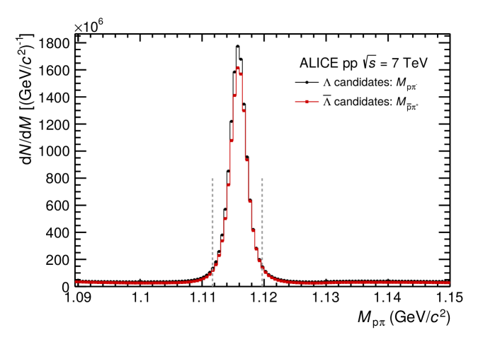
Figure 1: (Color online) Invariant mass distribution of $\mathrm{p}\pi^{-}$ ($\overline{\mathrm{p}}\pi^{+}$) to obtain the $\Lambda$ ($\overline{\Lambda}$ ) signal. The dashed lines set the selection width used in the analysis.

3 The correlation function

The observable of interest in femtoscopy is the two-particle correlation function, which is defined as the probability to find simultaneously two particles with momenta $\mathbf{p}_{1}$ and $\mathbf{p}_{2}$ divided by the product of the corresponding single particle probabilities

$$C(\mathbf{p}_{1},\mathbf{p}_{2})\equiv\frac{P(\mathbf{p}_{1},\mathbf{p}_{2})}{P(\mathbf{p}_{1})\cdot P(\mathbf{p}_{2})}.$$ (1)

These probabilities are directly related to the inclusive Lorentz invariant spectra $P(\mathbf{p}_{1},\mathbf{p}_{2})=E_{1}E_{2}\frac{\mathrm{d}^{6}N}{\mathrm{d}^{3}p_{1}\mathrm{d}^{3}p_{2}}$ and $P(\mathbf{p}_{1,2})=E_{1,2}\frac{\mathrm{d}^{3}N}{\mathrm{d}^{3}p_{1,2}}$. In absence of a correlation signal the value of $C(\mathbf{p}_{1},\mathbf{p}_{2})$ equals unity.

Approximating the emission process and the momenta of the particles, the size of the particle emitting source can be studied. Following [2], Eq. (1) can then be rewritten as

$$C(\mathbf{k^{*}})=\int\,d^{3}r^{*}S(r^{*})|\psi(r^{*},\mathbf{k^{*}})|^{2},$$ (2)

where $k^{*}$ is the relative momentum of the pair defined as $k^{*}=\frac{1}{2}\cdot|\mathbf{p}^{*}_{1}-\mathbf{p}^{*}_{2}|$, with $\mathbf{p}^{*}_{1}$ and $\mathbf{p}^{*}_{2}$ the momenta of the two particles in the pair rest frame (PRF, denoted by the ^∗), $S(r^{*})$ contains the distribution of the relative distance of particle pairs in the pair rest frame, the so-called source function, and $\psi(r^{*},\mathbf{k^{*}})$ denotes the relative wave function of the particle pair. The latter contains the particle interaction term and determines the shape of the correlation function. In this work, the p–p correlation function, which is theoretically well understood, is employed to obtain the required information about the source function and this information will be used to study the p–$\Lambda$ and $\Lambda$–$\Lambda$ interaction.

In order to relate the correlation function to experimentally accessible quantities, Eq. (1) is reformulated [2] as

$$C(k^{*})=\mathcal{N}\frac{A(k^{*})}{B(k^{*})},$$ (3)

The distribution of particle pairs from the same event is denoted with $A(k^{*})$ and $B(k^{*})$ is a reference sample of uncorrelated pairs. The latter is obtained using event mixing techniques, in which the particle pairs of interest are combined from single particles from different events. To avoid acceptance effects of the detector system, the mixing procedure is conducted only between particle pairs stemming from events with similar $z$ position of the primary vertex and similar multiplicity [2]. The normalization parameter for mixed and same event yields $\mathcal{N}$ is chosen such that the mean value of the correlation function equals unity for $k^{*}\in[0.2,~{}0.4]$ GeV/$c$.

As correlation functions of all studied baryon–baryon pairs, i.e. p–p , p–$\Lambda$ and $\Lambda$–$\Lambda$ , exhibit identical behavior compared to those of their respective anti-baryon–anti-baryon pairs, the corresponding samples are combined to enhance the statistical significance. Therefore, in the following p–p denotes the combination of $\mbox{p--p}\oplus\overline{\mathrm{p}}\mbox{--}\overline{\mathrm{p}}$, and accordingly for p–$\Lambda$ and $\Lambda$–$\Lambda$ .

3.1 Decomposition of the correlation function

The experimental determination of the correlation function is distorted by two distinct mechanisms. The sample of genuine particle pairs include misidentified particles and feed-down particles from strong and weak decays.

In this work a new method to separate all the individual components contributing to a measured correlation signal is proposed. The correlation functions arising from resonances or impurities of the sample are weighted with the so-called $\lambda$ parameters and in this way are taken into account in the total correlation function of interest

$$C(k^{*})=1+\lambda_{\mathrm{genuine}}\cdot(C_{\mathrm{genuine}}(k^{*})-1)+\sum_{ij}\lambda_{ij}(C_{ij}(k^{*})-1),$$ (4)

where the $i,j$ denote all possible impurity and feed-down contributions. These $\lambda$ parameters can be obtained employing exclusively single particle properties such as the purity and feed-down probability. The underlying mathematical formalism is outlined in App. A.

For the case of p–p correlation the following contributions must be taken into account

$$\begin{split}\{\mathrm{pp}\}=&~{}\mathrm{pp+p_{\Lambda}p+p_{\Lambda}p_{\Lambda}+p_{\Sigma^{+}}p+p_{\Sigma^{+}}p_{\Sigma^{+}}}\\ &\mathrm{+p_{\Lambda}p_{\Sigma^{+}}+\tilde{p}p+\tilde{p}p_{\Lambda}+\tilde{p}p_{\Sigma^{+}}+\tilde{p}\tilde{p}},\end{split}$$ (5)

where $\tilde{X}$ refers to misidentified particles of specie $X$. p_Λ and p${}_{\Sigma^{+}}$ correspond to protons stemming from the weak decay of the corresponding hyperons. The $\Xi\rightarrow\Lambda\pi\rightarrow p\pi\pi$ decays are explicitly considered in the feed-down contribution of the p–$\Lambda$ correlation and hence are omitted in Eq. (5) to avoid double counting. As shown in App. A, the fraction of primary protons and their feed-down fractions are required to calculate the $\lambda$ parameters of the different contributions to Eq. (5). The information about the origin of the protons, i.e. whether the particles are of primary origin, originating from feed-down or from the interactions with the detector material, is obtained by fitting Monte Carlo (MC) templates to the experimental distributions of the distance of closest approach of the track to the primary vertex. The MC templates and the purity are extracted from Pythia [61] simulations using the Perugia 2011 tune [62], which were filtered through the ALICE detector and the reconstruction algorithm [54]. The $p_{\mathrm{T}}$ averages are then calculated by weighting the quantities of interest by the respective particle yields d$N$/d$p_{\mathrm{T}}$. The resulting fraction of primary protons averaged over $p_{\mathrm{T}}$ is 87 % (where in this fraction we also include the protons stemming from strong decays of broad resonances), with the other 13 % of the total yield associated to weak decays of resonances and the contribution from the detector material is found to be negligible.

The feed-down from weakly decaying resonances is evaluated by using cross sections from Pythia and for the proton sample consists of the $\Lambda$ (70 %) and $\Sigma^{+}$ (30 %) contributions. The individual contributions to the total correlation function are presented in Tab. 2.

The decomposition of the p–$\Lambda$ correlation function is conducted in a similar manner as for the p–p pair, however considering the purities and feed-down fractions of both particles

$$\begin{split}\{\mathrm{p}\Lambda\}=&~{}\mathrm{p}\Lambda+\mathrm{p}\Lambda_{\Xi^{-}}+\mathrm{p}\Lambda_{\Xi^{0}}+\mathrm{p}\Lambda_{\Sigma^{0}}+\mathrm{p}_{\Lambda}\Lambda+\mathrm{p}_{\Lambda}\Lambda_{\Xi^{-}}+\mathrm{p}_{\Lambda}\Lambda_{\Xi^{0}}+\mathrm{p}_{\Lambda}\Lambda_{\Sigma^{0}}\\ &+\mathrm{p}_{\Sigma^{+}}\Lambda+\mathrm{p}_{\Sigma^{+}}\Lambda_{\Xi^{-}}+\mathrm{p}_{\Sigma^{+}}\Lambda_{\Xi^{0}}+\mathrm{p}_{\Sigma^{+}}\Lambda_{\Sigma^{0}}+\tilde{\mathrm{p}}\Lambda+\tilde{\mathrm{p}}\Lambda_{\Xi^{-}}+\tilde{\mathrm{p}}\Lambda_{\Xi^{0}}+\tilde{\mathrm{p}}\Lambda_{\Sigma^{0}}\\ &+\mathrm{p}\tilde{\Lambda}+\mathrm{p}_{\Lambda}\tilde{\Lambda}+\mathrm{p}_{\Sigma^{+}}\tilde{\Lambda}+\tilde{\mathrm{p}}\tilde{\Lambda}.\end{split}$$ (6)

The $\Lambda$ purity is obtained from fits to the invariant mass spectra in eight bins of $p_{\mathrm{T}}$ and defined as $S/(S+B)$, where $S$ denotes the actual signal and $B$ the background. The feed-down contribution is determined from MC template fits of the experimental distributions of the cosine pointing angle, in which a total of four templates are considered corresponding to direct, feed-down, material and impurity contributions. The production probability d$N$/d$p_{\mathrm{T}}$ is employed in order to obtain $p_{\mathrm{T}}$ weighted average values.
Around $73\%$ of the $\Lambda$s are primaries (where in this fraction we also include the $\Lambda$ stemming from strong decays of broad resonances) and $23\%$ originate from weakly decaying resonances, which is in line with the values quoted in [63]. The remaining yield is associated to combinatorial background and $\Lambda$s produced in the detector material. The main contribution to the feed-down fraction is expected to originate from the $\Xi$ states with no preference for the neutral or the charged, respectively. This hypothesis is supported by Pythia simulations where the secondary $\Lambda$ particles arise from the weak decay of the $\Xi^{0}$ ($48\%$) and $\Xi^{\mathrm{\pm}}$ ($49\%$) resonances. The remaining contribution in the simulation arises from the $\Sigma^{0}$, which however is treated separately. Since the latter decays electromagnetically almost exclusively into $\Lambda\gamma$ [59], it has a very short life time and cannot be experimentally differentiated from the sample of primary $\Lambda$s. Measurements of the ratio $R_{\Sigma^{0}/\Lambda}=\sigma_{\Sigma^{0}}/\sigma_{\Lambda}$ have obtained values around 1/3 [64, 65, 66, 67], however with large uncertainties for hadronic collisions at high energies. For lack of better estimates the value of 1/3 is used in the following. The resulting $\lambda$ parameters for the p–$\Lambda$ pair are shown in Tab. 2.

For the $\Lambda$–$\Lambda$ correlation function the following pair contributions are taken into account

$$\begin{split}\{\Lambda\Lambda\}=&~{}\Lambda\Lambda+\Lambda\Lambda_{\Sigma^{0}}+\Lambda_{\Sigma^{0}}\Lambda_{\Sigma^{0}}+\Lambda\Lambda_{\Xi^{0}}+\Lambda_{\Xi^{0}}\Lambda_{\Xi^{0}}+\Lambda\Lambda_{\Xi^{-}}\\ &+\Lambda_{\Xi^{-}}\Lambda_{\Xi^{-}}+\Lambda_{\Sigma^{0}}\Lambda_{\Xi^{0}}+\Lambda_{\Sigma^{0}}\Lambda_{\Xi^{-}}+\Lambda_{\Xi^{0}}\Lambda_{\Xi^{-}}\\ &+\tilde{\Lambda}\Lambda+\tilde{\Lambda}\Lambda_{\Sigma^{0}}+\tilde{\Lambda}\Lambda_{\Xi^{-}}+\tilde{\Lambda}\Lambda_{\Xi^{0}}+\tilde{\Lambda}\tilde{\Lambda}.\end{split}$$ (7)

The resulting $\lambda$ parameters are shown in Tab. 2. Notable is that the actual pair of interest contributes only to about one third of the signal, while pair fractions involving in particular $\Sigma^{0}$ and $\Xi$ give a significant contribution. The statistical uncertainties of these parameters are negligible and their influence on the systematic uncertainties will be evaluated in Sec. 4.

p–p		p–$\Lambda$		$\Lambda$–$\Lambda$
Pair	$\lambda$ parameter [%]	Pair	$\lambda$ parameter [%]	Pair	$\lambda$ parameter [%]
pp	74.18	p$\Lambda$	47.13	$\Lambda\Lambda$	29.94
pΛp	15.52	p$\Lambda_{\Xi^{-}}$	9.92	$\Lambda\Lambda_{\Sigma^{0}}$	19.96
pΛpΛ	0.81	p$\Lambda_{\Xi^{0}}$	9.92	$\Lambda_{\Sigma^{0}}\Lambda_{\Sigma^{0}}$	3.33
p${}_{\Sigma^{+}}$p	6.65	p$\Lambda_{\Sigma^{0}}$	15.71	$\Lambda\Lambda_{\Xi^{0}}$	12.61
p${}_{\Sigma^{+}}$p${}_{\Sigma^{+}}$	0.15	p${}_{\Lambda}\Lambda$	4.93	$\Lambda_{\Xi^{0}}\Lambda_{\Xi^{0}}$	1.33
pΛp${}_{\Sigma^{+}}$	0.70	p${}_{\Lambda}\Lambda_{\Xi^{-}}$	1.04	$\Lambda\Lambda_{\Xi^{-}}$	12.61
$\tilde{\mathrm{p}}$p	1.72	p${}_{\Lambda}\Lambda_{\Xi^{0}}$	1.04	$\Lambda_{\Xi^{-}}\Lambda_{\Xi^{-}}$	1.33
$\tilde{\mathrm{p}}$pΛ	0.18	p${}_{\Lambda}\Lambda_{\Sigma^{0}}$	1.64	$\Lambda_{\Sigma^{0}}\Lambda_{\Xi^{0}}$	4.20
$\tilde{\mathrm{p}}$p${}_{\Sigma^{+}}$	0.08	p${}_{\Sigma^{+}}\Lambda$	2.11	$\Lambda_{\Sigma^{0}}\Lambda_{\Xi^{-}}$	4.20
$\tilde{\mathrm{p}}\tilde{\mathrm{p}}$	0.01	p${}_{\Sigma^{+}}\Lambda_{\Xi^{-}}$	0.44	$\Lambda_{\Xi^{0}}\Lambda_{\Xi^{-}}$	2.65
		p${}_{\Sigma^{+}}\Lambda_{\Xi^{0}}$	0.44	$\tilde{\Lambda}\Lambda$	4.38
		p${}_{\Sigma^{+}}\Lambda_{\Sigma^{0}}$	0.70	$\tilde{\Lambda}\Lambda_{\Sigma^{0}}$	1.46
		$\tilde{\mathrm{p}}\Lambda$	0.55	$\tilde{\Lambda}\Lambda_{\Xi^{0}}$	0.92
		$\tilde{\mathrm{p}}\Lambda_{\Xi^{-}}$	0.18	$\tilde{\Lambda}\Lambda_{\Xi^{-}}$	0.92
		$\tilde{\mathrm{p}}\Lambda_{\Xi^{0}}$	0.12	$\tilde{\Lambda}\tilde{\Lambda}$	0.16
		$\tilde{\mathrm{p}}\Lambda_{\Sigma^{0}}$	0.12
		p$\tilde{\Lambda}$	3.45
		p${}_{\Lambda}\tilde{\Lambda}$	0.36
		p${}_{\Sigma^{+}}\tilde{\Lambda}$	0.15
		$\tilde{\mathrm{p}}\tilde{\Lambda}$	0.04

Table 2: Weight parameters of the individual components of the p–p , p–$\Lambda$ and $\Lambda$–$\Lambda$ correlation function.

Possible effects that were considered in this analysis and that could be influencing the source are either the decay of strong resonances, or a $m_{\mathrm{T}}$ scaling. The latter is related to collective effects and may result in a non-Gaussian behavior of the source. The p–p correlation function is here considered as a benchmark since the theoretical description of the interaction is well established. The good agreement between the $m_{\mathrm{T}}$-integrated data and the femtoscopic fit demonstrates that the assumption of a Gaussian source is pertinent. A comparison of the $m_{\mathrm{T}}$ distribution for p–p and p–$\Lambda$ pairs shows a good agreement between the two. The limited experimental sample, however, does not allow conducting a differential analysis yet.
Additionally, we have considered the effect of the strong decays such as $\Delta\rightarrow N+\pi$ and $N^{*}\rightarrow\Lambda+K$ on the production of protons and $\Lambda$. Since the $\Delta$ and $N^{*}$ resonances have typical widths above 120 MeV the decay length is in the order of 1 fm so that the decay particles do still experience the final state interaction with the neighbouring particles as the primaries do. We estimate that about 65% of all primary protons and $\Lambda$ stem from the strong decay of resonances [68] and we have simulated how the source could be modified by such effects. A difference of 5% in the results of the Gaussian fit is found when comparing p–p to p–$\Lambda$ pairs. These effects are in the same order of the present uncertainty on the radius and are herewith neglected. A quantitative study including all resonances is planned in the analysis of the LHC Run 2 sample.

3.2 Detector effects

The shape of the experimentally determined correlation function is affected by the finite momentum resolution. This is taken into account when the experimental data are compared to model calculations in the fitting procedure by transforming the modeled correlation function, see Eq. (15), to the reconstructed momentum basis.

When tracks of particle pairs involved in the correlation function are almost collinear, i.e. have a low $k^{*}$, detector effects can affect the measurement. No hint for track merging or splitting is found and therefore no explicit selection criteria are introduced.

3.3 Non-femtoscopic background

For sufficiently large relative momenta ($k^{*}>200$ MeV/$c$) and increasing separation distance, the FSI among the particles is suppressed and hence the correlation function should approach unity. As shown in Fig. 2, however, the measured correlation function for p–p and p–$\Lambda$ exhibits an increase for $k^{*}$ larger than about $200$ MeV/$c$ for the two systems. Such non-femtoscopic effects, probably due to energy-momentum conservation, are in general more pronounced in small colliding systems where the average particle multiplicity is low  [2]. In the case of meson–meson correlations at ultra-relativistic energies, the appearance of long-range structures in the correlation functions for moderately small $k^{*}$ ($k^{*}<200$ MeV/c) is typically interpreted as originating from mini-jet-like structures  [50, 69].

Pythia also shows the same non-femtoscopic correlation for larger $k^{*}$ but fails to reproduce quantitatively the behavior shown in Fig. 2, as already observed for the angular correlation of baryon–baryon and anti-baryon–anti-baryon pairs [58].

Energy-momentum conservation leads to a contribution to the signal which can be reproduced with a formalism described in [70] and is accordingly also considered in this work. Therefore, a linear function $C(k^{*})_{\mathrm{non-femto}}=ak^{*}+b$ where $a,b$ are fit parameters, is included to the global fit as $C(k^{*})=C(k^{*})_{\mathrm{femto}}\times C(k^{*})_{\mathrm{non-femto}}$ to improve the description of the signal by the femtoscopic model. The fit parameters of the baseline function are obtained in $k^{*}\in[0.3,~{}0.5]$ GeV/$c$ for p–p and p–$\Lambda$ pairs. For the case of the $\Lambda$–$\Lambda$ correlation function, the uncertainties of the data do not allow to additionally add a baseline, which is therefore omitted in the femtoscopic fit.

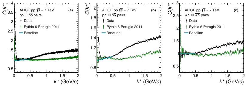
Figure 2: (Color online) The raw correlation function compared to Pythia 6 Perugia 2011 simulations for p–p (a), p–$\Lambda$ (b) and $\Lambda$–$\Lambda$ (c) pairs.

3.4 Modeling the correlation function

3.4.1 Genuine correlation function

For the p–p correlation function the Coulomb and the strong interaction as well as the antisymmetrization of the wave functions are considered [71]. The strong interaction part of the potential is modeled employing the Argonne $v_{18}$ [52] potential considering the $s$ and $p$ waves. The source is assumed to be isotropic with a Gaussian profile of radius $r_{0}$. The resulting Schrödinger equation is then solved with the CATS [53].

In the case of p–$\Lambda$ and $\Lambda$–$\Lambda$ we employ the Lednický and Lyuboshitz analytical model [72] to describe these correlation functions. This model is based on the assumption of an isotropic source with Gaussian profile

$$S(r_{0})=\frac{1}{(4\pi r_{0}^{2})^{3/2}}\text{exp}\left(-\frac{r^{2}}{4r_{0}^{2}}\right),$$ (8)

where $r_{0}$ is the size of the source. Additionally, the complex scattering amplitude is evaluated by means of the effective range approximation

$$f(k^{*})^{S}=\left(\frac{1}{f_{0}^{S}}+\frac{1}{2}d_{0}^{S}k^{*2}-ik^{*}\right)^{-1},$$ (9)

with the scattering length $f_{0}^{S}$, the effective range $d_{0}^{S}$ and $S$ denoting the total spin of the particle pair. In the following, the usual sign convention of femtoscopy is employed where an attractive interaction leads to a positive scattering length. With these assumptions the analytical description of the correlation function for uncharged particles [72] reads

$$C(k^{*})_{\rm{Lednicky}}=1+\sum_{S}\rho_{S}\left[\frac{1}{2}\left|\frac{f(k^{*})^{S}}{r_{0}}\right|^{2}\left(1-\frac{d_{0}^{S}}{2\sqrt{\pi}r_{0}}\right)+\frac{2\Re{f(k^{*})^{S}}}{\sqrt{\pi}r_{0}}F_{1}(Q_{\rm{inv}}r_{0})-\frac{\Im{f(k^{*})^{S}}}{r_{0}}F_{2}(Q_{\rm{inv}}r_{0})\right],$$ (10)

where $\Re{f(k^{*})^{S}}$ ($\Im{f(k^{*})^{S}}$) denotes the real (imaginary) part of the complex scattering amplitude, respectively. The $F_{1}(Q_{\rm{inv}}r_{0})$ and $F_{2}(Q_{\rm{inv}}r_{0})$ are analytical functions resulting from the approximation of isotropic emission with a Gaussian source and the factor $\rho_{S}$ contains the pair fraction emitted into a certain spin state $S$. For the p–$\Lambda$ pair unpolarized emission is assumed.

The $\Lambda$–$\Lambda$ pair is composed of identical particles and hence additionally quantum statistics needs to be considered, which leads to the introduction of an additional term to the Lednický model, as employed e.g. in [16].

While the CATS framework can provide an exact solution for any source and local interaction potential, the Lednicky-Lyuboshitz approach uses the known analytical solution outside the range of the strong interaction potential and takes into account its modification in the inner region in an approximate way only. That is why this approach may not be valid for small systems.

3.4.2 Residual correlations

Table 2 demonstrates that a significant admixture of residuals is present in the experimental sample of particle pairs. A first theoretical investigation of these so-called residual correlations was conducted in [73]. This analysis relies on the procedure established in [19], where the initial correlation function of the residual is calculated and then transformed to the new momentum basis after the decay.

For the p–p channel only the feed-down from the p–$\Lambda$ correlation function is considered, which is obtained by fitting the p–$\Lambda$ experimental correlation function and then transforming it to the p–p momentum basis. All contributions are weighted by the corresponding $\lambda$ parameters and the modeled correlation function for this pair $C_{model,\mathrm{p\mbox{--}p}}(k^{*})$ can be written as

$$C_{model,\mathrm{p\mbox{--}p}}(k^{*})=1+\lambda_{\mathrm{pp}}\cdot(C_{\mathrm{pp}}(k^{*})-1)+\lambda_{\mathrm{pp}_{\Lambda}}(C_{\mathrm{pp}_{\Lambda}}(k^{*})-1).$$ (11)

All other residual correlations are assumed to be flat.

For the p–$\Lambda$ , residual correlations from the p–$\Sigma^{0}$ , p–$\Xi$ and $\Lambda$–$\Lambda$ pairs are taken into account. As the $\Lambda$–$\Lambda$ correlation function is rather flat no further transformation is applied. The p–$\Sigma^{0}$ correlation function is obtained using predictions from [74].

As the decay products of the reaction $\Xi\rightarrow\Lambda\pi$ are charged and therefore accessible by ALICE, we measure the p–$\Xi$ correlation function. The experimental data are parametrized with a phenomenological function

$$C_{\mathrm{p\mbox{--}}\Xi^{-}}(k^{*})=1+\frac{\exp(-k^{*}a_{\Xi})}{k^{*}a_{\Xi}},$$ (12)

where the parameter $a_{\Xi}$ is employed to scale the function to the data and has no physical meaning. Its value is found to be $a_{\Xi}=3.88$ fm.

The modeled correlation function $C_{model,\mathrm{p}\mbox{--}\Lambda}(k^{*})$ for the pair is obtained by

$$C_{model,\mathrm{p}\mbox{--}\Lambda}(k^{*})=1+\lambda_{\mathrm{p}\Lambda}(C_{\mathrm{p}\Lambda}(k^{*})-1)+\lambda_{\mathrm{p}\Lambda_{\Sigma^{0}}}(C_{\mathrm{p}\Lambda_{\Sigma^{0}}}(k^{*})-1)+\lambda_{\mathrm{p}\Lambda_{\Xi^{-}}}(C_{\mathrm{p}\Lambda_{\Xi^{-}}}(k^{*})-1).$$ (13)

As the present knowledge on the hyperon–hyperon interaction is scarce, in particular regarding the interaction of the $\Lambda$ with other hyperons, all residual correlations feeding into the $\Lambda$–$\Lambda$ correlation function are considered to be consistent with unity,

$$C_{model,\Lambda\mbox{--}\Lambda}(k^{*})=1+\lambda_{\Lambda\Lambda}(C_{\Lambda\Lambda}(k^{*})-1).$$ (14)

It should be noted, that the residual correlation functions, after weighting with the corresponding $\lambda$ parameter, transformation to the momentum base of the correlation of interest and taking into account the finite momentum resolution, only barely contribute to the total fit function.

3.4.3 Total correlation function model

The correlation function modeled according to the considerations discussed above is then multiplied by a linear function to correct for the baseline as discussed in Sec. 3.3 and weighted with a normalization parameter $\mathcal{N}$

$$C_{tot}(k^{*})=\mathcal{N}\cdot(a+b\cdot k^{*})\cdot C_{model}(k^{*}),$$ (15)

where $C_{model}(k^{*})$ incorporates all considered theoretical correlation functions, weighted with the corresponding $\lambda$ parameters as discussed in Sec. 3.1 and 3.4.

The inclusion of a baseline is further motivated by the presence of a linear but non-flat correlation observed in the data outside the femtoscopic region (see Fig. 2 for $k^{*}\in[0.3,~{}0.5]$ GeV/$c$). When attempting to use a higher order polynomial to model the background, the resulting curves are still compatible with a linear function, while their interpolation into the lower $k^{*}$ region leads to an overall poorer fit quality.

4 Systematic uncertainties

4.1 Correlation function

The systematic uncertainties of the correlation functions are extracted by varying the proton and $\Lambda$ candi-date selection criteria according to Tab. 3. Due to the low number of particle pairs, in particular at low $k^{*}$, the resulting variations of the correlation functions are in general much smaller than the statistical uncertainties. In order to still estimate the systematic uncertainties the data are rebinned by a factor of 10. The systematic uncertainty on the correlation function is obtained by computing the ratio of the default correlation function to the one obtained by the respective cut variation. Whenever this results in two systematic uncertainties, i.e. by a variation up and downwards, the average is taken into account. Then all systematic uncertainties from the cut variations are summed up quadratically. This is then extrapolated to the finer binning of the correlation function by fitting a polynomial of second order. The obtained systematic uncertainties are found to be largest in the lowest $k^{*}$ bin. The individual contributions in that bin are summarized in Tab. 3 and the resulting total systematic uncertainty accounts to about 4 % for p–p , 1 % for p–$\Lambda$ and 2.5 % for $\Lambda$–$\Lambda$ . Variations of the proton DCA selection are not taken into account for the computation of the systematic uncertainty since it dilutes (enhances) the correlation signal by introducing more (less) secondaries in the sample. This effect is recaptured by a change in the $\lambda$ parameter.

Variable	Default	Variation	p–p [%]	p–$\Lambda$ [%]	$\Lambda$–$\Lambda$ [%]
Min. $p_{\mathrm{T}}$ proton ($\mathrm{GeV}\kern-0.50003pt/\kern-0.20004ptc\,$)	0.5	0.4, 0.6	1	0.2	-
$|\eta|$ proton	0.8	0.7, 0.9	0.4	0.2	-
$n_{\sigma}$ proton	3	2, 5	1.8	0.2	-
Proton tracks	TPC only	Global	2.4	0	-
$n_{\mathrm{Cluster}}$ proton	80	90	0.3	0.1	-
Min. $p_{\mathrm{T}}$ $V_{0}$ ($\mathrm{GeV}\kern-0.50003pt/\kern-0.20004ptc\,$)	0.3	0.24, 0.36	-	0	0
cos$(\alpha)$ $V_{0}$	0.99	0.998	-	0	1.8
$n_{\sigma}$ $V_{0}$ daughter	5	4	-	0.1	0.3
$n_{\mathrm{Cluster}}$ $V_{0}$ daughter	70	80	-	0.1	0.7
$|\eta|$ $V_{0}$	0.8	0.7, 0.9	-	0.6	0.8
$\mathrm{DCA}(|p,\pi|)$ (cm)	1.5	1.2	-	0.5	0
$\mathrm{DCA}$ (cm)	0.05	0.06	-	0.7	0.6

Table 3: Selection parameter variation and the resulting relative systematic uncertainty on the p–p , p–$\Lambda$ and $\Lambda$–$\Lambda$ correlation function.

4.2 Femtoscopic fit

To evaluate the systematic uncertainty of the femtoscopic fit, and hence on the measurement of the radius $r_{0}$, the fit is performed applying the following variations. Instead of the common fit, the radius is determined separately from the p–p and p–$\Lambda$ correlation functions. $\Lambda$–$\Lambda$ is excluded because it imposes only a shallow constraint on the radius, in particular since the scattering parameters are unconstrained for the fit. Furthermore, the input to the $\lambda$ parameters are varied by 25 %, while keeping the purity and the fraction of primaries and secondaries constant since this would correspond to a variation of the particle selection and thus would require a different experimental sample as discussed above. Additionally, all fit ranges of both the femtoscopic and the baseline fits are varied individually by up to 50 % and 10 %, respectively. The lower bound of the femtoscopic fit is always left at its default value. For the p–$\Lambda$ correlation function the dependence on the fit model is studied by replacing the Lednický and Lyuboshitz analytical model with the potential introduced by Bodmer, Usmani, and Carlson [75] for which the Schrödinger equation is explicitly solved using CATS. Additionally, the fit for the p–p and p–$\Lambda$ correlation function is performed without the linear baseline. The radius is determined for 2000 random combinations of the above mentioned variations. The resulting distribution of radii is not symmetric and the systematic uncertainty is therefore extracted as the boundaries of the 68 % confidence interval around the median of the distribution and accounts to about 4 % of the determined radius.

5 Results

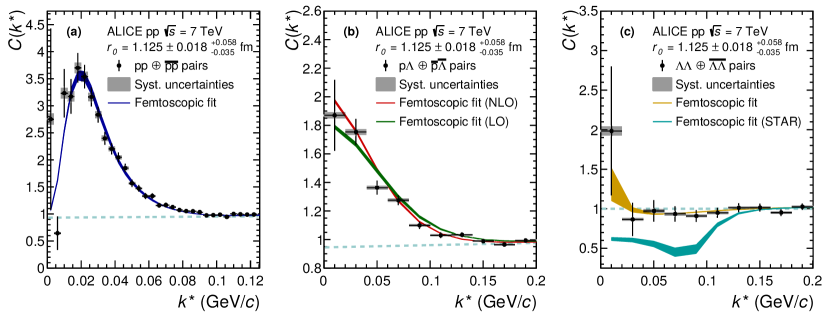
Figure 3: (Color online) The p–p (a), p–$\Lambda$ (b) and $\Lambda$–$\Lambda$ (c) correlation function with a simultaneous fit with the NLO expansion (red line) for the scattering parameter of p–$\Lambda$  [26]. The dashed line denotes the linear baseline. After the fit is performed the LO [25] parameter set (green curve) is plugged in for the p–$\Lambda$ system and the scattering length obtained from [16] for the $\Lambda$–$\Lambda$ system (cyan curve).

The obtained p–p , p–$\Lambda$ and $\Lambda$–$\Lambda$ correlation functions are shown in Fig. 3. For each of the correlation functions we do not observe any mini-jet background in the low $k^{*}$ region, as observed in the case of neutral [76] and charged [51] kaon pairs and charged pion pairs [50]. This demonstrates that the femtoscopic signal in baryon–baryon correlations is dominant in ultrarelativistic $\mathrm{p\kern-0.50003ptp}$ collisions. The signal amplitude for the p–p and p–$\Lambda$ correlations are much larger than the one observed in analogous studies from heavy-ion collisions [1, 12, 13, 15], due to the small particle emitting source formed in $\mathrm{p\kern-0.50003ptp}$ collisions, allowing a higher sensitivity to the FSI.

In absence of residual contributions and any FSI, the $\Lambda$–$\Lambda$ correlation function is expected to approach 0.5 as $k^{*}$ $\rightarrow$ 0. While the data suggest that the $\Lambda$–$\Lambda$ correlation exceeds the value expected considering only quantum statistic effects, the limited amount of data of the herewith presented sample does not allow to draw strong conclusions on the attractive nature of the $\Lambda$–$\Lambda$ interaction [27, 38].

The experimental data are fitted using CATS and hence the exact solution of the Schrödinger equation for the $\mathrm{p\kern-0.50003ptp}$ correlation and the Lednický model for the p–$\Lambda$ and $\Lambda$–$\Lambda$ correlation. The three fits are done simultaneously and this way the source radius is extracted and different scattering parameters for the p–$\Lambda$ and $\Lambda$–$\Lambda$ interactions can be tested. While in the case of the p–p and p–$\Lambda$ correlation function the existence of a baseline is clearly visible in the data, the low amount of pairs in the $\Lambda$–$\Lambda$ channel do not allow for such a conclusion. Therefore, the baseline is not included in the model for the $\Lambda$–$\Lambda$ correlation function.

The simultaneous fit is carried out by using a combined $\chi^{2}$ and with the radius as a free parameter common to all correlation functions. The fit range is $k^{*}$ $\in[0,~{}0.16]$ GeV/$c$ for p–p and $k^{*}$ $\in[0,~{}0.22]$ GeV/$c$ for p–$\Lambda$ and $\Lambda$–$\Lambda$ . Hereafter we adopt the convention of positive scattering lengths for attractive interactions and negative scattering lengths for repulsive interactions. The p–$\Lambda$ strong interaction is modeled employing scattering parameters obtained using the next-to-leading order expansion of a chiral effective field theory at a cutoff scale of $\Lambda=600$ MeV [26]. The simultaneous fit of the p–p , p–$\Lambda$ and $\Lambda$–$\Lambda$ correlation functions yields a common radius of $r_{0}=1.125\pm 0.018\,\mathrm{(stat)}\,^{+0.058}_{-0.035}\,\mathrm{(syst)}$ fm.

The blue line in the left panel in Fig. 3 shows the result of the femtoscopic fit to the p–p correlation function using the Argonne $v_{18}$ potential that describes the experimental data in a satisfactory way. The red curve in the central panel shows the result of the NLO calculation for p–$\Lambda$ . In the case of $\Lambda$–$\Lambda$ (right panel), the yellow curve represents the femtoscopic fit with free scattering parameters. The width of the femtoscopic fits corresponds to the systematic uncertainty of the correlation function discussed in Sec. 4.

After the fit with the NLO scattering parameters has converged, the p–$\Lambda$ correlation function for the same source size is compared to the data using various theoretically obtained scattering parameters [77, 78, 79, 80, 81, 25, 26, 82, 83] as summarized in Tab. 4. The degree of consistency is expressed in the number of standard deviations $n_{\sigma}$. The employed models include several versions of meson exchange models proposed such as the Nijmegen model D (ND) [77], model F (NF) [78], soft core (NSC89 and NSC97) [79, 80] and extended soft core (ESC08) [81]. Additionally, models considering contributions from one- and two-pseudoscalar-meson exchange diagrams and from four-baryon contact terms in $\chi$EFT at leading [25] and next-to-leading order [26] are employed, together with the first version of the Jülich Y–N meson exchange model [82], which in a later version [83] also features one-boson exchange.

All employed models describe the data equally well and hence the available data does not allow yet for a discrimination. As an example, we show in the central panel of Fig. 3 how employing scattering parameters different than the NLO ones reflects on the p–$\Lambda$ correlation function. The green curve corresponds to the results obtained employing LO scattering parameters and the theoretical correlation function is clearly sensitive for $k^{*}$ $\rightarrow$ 0 to the input parameter.

Model		$f_{0}^{S=0}$ (fm)	$f_{0}^{S=1}$ (fm)	$d_{0}^{S=0}$ (fm)	$d_{0}^{S=1}$ (fm)	$n_{\sigma}$
ND [77]		1.77	2.06	3.78	3.18	1.1
NF [78]		2.18	1.93	3.19	3.358	1.1
NSC89 [79]		2.73	1.48	2.87	3.04	0.9
NSC97 [80]	a	0.71	2.18	5.86	2.76	1.0
	b	0.9	2.13	4.92	2.84	1.0
	c	1.2	2.08	4.11	2.92	1.0
	d	1.71	1.95	3.46	3.08	1.0
	e	2.1	1.86	3.19	3.19	1.1
	f	2.51	1.75	3.03	3.32	1.0
ESC08 [81]		2.7	1.65	2.97	3.63	0.9
$\chi$EFT	LO [25]	1.91	1.23	1.4	2.13	1.8
	NLO [26]	2.91	1.54	2.78	2.72	1.5
Jülich	A [82]	1.56	1.59	1.43	3.16	1.0
	J04 [83]	2.56	1.66	2.75	2.93	1.4
	J04c [83]	2.66	1.57	2.67	3.08	1.1

Table 4: Scattering parameters for the p–$\Lambda$ system from various theoretical calculations [77, 78, 79, 80, 81, 25, 26, 82, 83] and the corresponding degree of consistency with the experimentally determined correlation function expressed in numbers of standard deviations $n_{\sigma}$. The $\chi$EFT scattering parameters are obtained at a cutoff scale $\Lambda=600$ MeV. The usual sign convention of femtoscopy is employed where an attractive interaction leads to a positive scattering length.

In order to probe which scattering parameters are compatible with the measured $\Lambda$–$\Lambda$ correlation function, the effective range and the scattering length of the potential are varied within $d_{0}\in[0,18]$ fm and $1/f_{0}\in[-2,5]$ 1/fm, while keeping the renormalization constant $\mathcal{N}$ as the only free fit parameter. It should be noted that the resulting variations of $\mathcal{N}$ are on the percent level. The resulting correlation functions obtained by employing the Lednický and Lyuboshitz analytical model [72] and considering also the secondaries and impurities contributions are compared to the data. The degree of consistency is expressed in the number of standard deviations $n_{\sigma}$, as displayed in Fig. 4 together with an overview of the present knowledge about the $\Lambda$ –$\Lambda$ interaction. For a detailed overview of the currently available models see e.g. [38], from which we have obtained the collection of scattering parameters. Additionally to the Nijmegen meson exchange models mentioned above, the data are compared to various other theoretical calculations. An exemplary boson-exchange potential is Ehime [84, 85], whose strength is fitted to the outdated double hypernuclear bound energy, $\Delta B_{\Lambda\Lambda}=4$ MeV [86] and accordingly known to be too attractive. As an exemplary quark model including baryon–baryon interactions with meson exchange effects, the fss2 model [87, 88] is used. Moreover, the potentials by Filikhin and Gal (FG) [89] and by Hiyama, Kamimura, Motoba, Yamada, and Yamamoto (HKMYY) [90], which are capable of describing the NAGARA event [36] are employed.

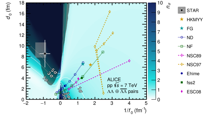
Figure 4: (Color online) Number of standard deviations $n_{\sigma}$ of the modeled correlation function for a given set of scattering parameters (effective range $d_{0}$ and scattering length $f_{0}$) with respect to the data, together with various model calculations [77, 78, 79, 80, 81, 84, 85, 87, 88, 89, 90] and measurements [16]. The gray shaded area corresponds to the region where the Lednický model predicts a negative correlation function for $\mathrm{p\kern-0.50003ptp}$ collisions at $\sqrt{s}=7\,$TeV.

In contrast to the p–$\Lambda$ case, the agreement with the data increases with every revision of the Nijmegen potential, while the introduction of the extended soft core slightly increases the deviation. In particular solution NSC97f yields the overall best agreement with the data. The correlation function modeled using scattering parameters of the Ehime model which is known to be too attractive deviates by about 2 standard deviations from the data.
For an attractive interaction (positive $f_{0}$) the correlation function is pushed from the quantum statistics distribution for two fermions (correlation function equal to $0.5$ for $k^{*}=\,0$) to unity. As a result within the current uncertainties the $\Lambda$–$\Lambda$ correlation function is rather flat and close to 1 and this lack of structure makes it impossible to extract the two scattering parameters with a reasonable uncertainty. This means that even by increasing the data by a factor $10$, as expected from the RUN2 data, it will be very complicated to constrain precisely the region $f_{0}>0$.
As for the region of negative scattering length $f_{0}$ this is connected in scattering theory either to a repulsive interaction or to the existence of a bound state close to the threshold and a change in the sign of the scattering length. Since the $\Lambda$–$\Lambda$ interaction is known to be slightly attractive above the threshold [36], the measurement of a negative scattering lengths would strongly support the existence of the H-dibaryon. Notably the correlation function modeled employing the scattering parameters obtained by the STAR collaboration in Au–Au collisions at $\sqrt{s_{\mathrm{NN}}}=200$ GeV [16] and all the secondaries and impurities contributions deviates by 6.8 standard deviations from the data. This is also shown by the cyan curve displayed in the right panel of Fig. 3 which is obtained using the source radius and the $\lambda$ parameters from this analysis and the scattering parameters from [16]. On the other hand these parameters and all those corresponding to the gray-shaded area in Fig. 4 lead to a negative genuine $\Lambda$–$\Lambda$ correlation function if the Lednický model is employed. The total correlation function that is compared to the experimental data is not negative because the impurities and secondaries contributions lead to a total correlation function that is always positive. This means that the combination of large effective ranges and negative scattering lengths translate into unphysical correlation functions, for small colliding systems as $\mathrm{p\kern-0.50003ptp}$. This effect is not immediate visible in larger colliding system such as Au–Au at $\sqrt{s_{\mathrm{NN}}}=200$ GeV measured by STAR, where the obtained correlation function does not become negative. This demonstrates that these scattering parameters intervals combined with the Lednický model are not suited to describe the correlations functions measured in small systems. One could test the corresponding local potentials with the help of CATS [53], since the latter does not suffer from the limitations of the Lednický model due to the employment of the asymptotic solution. On the other hand we have directly compared the correlation functions obtained employing CATS and the $\Lambda$–$\Lambda$ local potentials reported in [38] with the correlation functions obtained using the corresponding scattering parameters and the Lednický model. For the typical source radii of $1.3$ fm the deviations are within 10 %. This disfavours the region of negative scattering lengths and large effective ranges for the $\Lambda$–$\Lambda$ correlation.

This study is the first measurement with baryon pairs in $\mathrm{p\kern-0.50003ptp}$ collisions at $\sqrt{s}=7\,$TeV, while other femtoscopic analyses were conducted with neutral [76] and charged [51] kaon pairs and charged pion pairs [50] with the ALICE experiment. The radius obtained from baryon pairs is found to be slightly larger than that measured from meson-meson pairs at comparable transverse mass as shown in Fig. 5

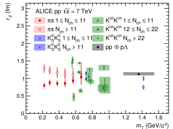
Figure 5: (Color online) Comparison of radii obtained for different charged particle multiplicity intervals in the $\mathrm{p\kern-0.50003ptp}$ collision system at $\sqrt{s}=7$ TeV [50, 51, 76]. The error bars correspond to statistical and the shaded regions to the systematic uncertainties. The black point is the radius obtained in this analysis with p–p , p–$\Lambda$ and $\Lambda$–$\Lambda$ pairs, while the gray bar corresponds to the range of covered $m_{\mathrm{T}}$ in this analysis.

6 Summary

This paper presents the first femtoscopic measurement of p–p , p–$\Lambda$ and $\Lambda$–$\Lambda$ pairs in $\mathrm{p\kern-0.50003ptp}$ collisions at $\sqrt{s}=7$ TeV. No evidence for the presence of mini-jet background is found and it is demonstrated that this kind of studies with baryon–baryon and anti-baryon–anti-baryon pairs are feasible. With a newly developed method to compute the contributions arising from impurities and weakly decaying resonances to the correlation function from single particles quantities only, the genuine correlation functions of interest can be extracted from the signal. These correlation functions contribute with 74 % for p–p , 47 % for p–$\Lambda$ and 30 % for $\Lambda$–$\Lambda$ to the total signal. A simultaneous fit of all correlation functions with a femtoscopic model featuring residual correlations stemming from the above mentioned effects yields a radius of the particles emitting source of $r_{0}=1.125\pm 0.018\,\mathrm{(stat)}\,^{+0.058}_{-0.035}\,\mathrm{(syst)}$ fm. For the first time, the Argonne $v_{18}$ $NN$ potential with the $s$ and $p$ waves was used to successfully describe the p–p correlation and in so obtain a solid benchmark for our investigation. For the case of the p–$\Lambda$ correlation function, the NLO parameter set obtained within the framework of chiral effective field theory is consistent with the data, but other models are also found to be in agreement with the data. The present pair data in the $\Lambda$–$\Lambda$ channel allows us to constrain the available scattering parameter space. Large effective ranges $d_{0}$ in combination with negative scattering parameters lead to unphysical correlations if the Lednický model is employed to compute the correlation function. This also holds true for the the average values published by the STAR collaboration in Au–Au collisions at $\sqrt{s_{\mathrm{NN}}}=200$ GeV, that are found to be incompatible with the measurement in $\mathrm{p\kern-0.50003ptp}$ collisions within the Lednický model.

The larger data sample of the LHC Run 2 and Run 3, where we expect up to a factor ten and 100 more data respectively, will enable us to extend the method also to $\Sigma$, $\Xi$ and $\Omega$ hyperons and thus further constrain the Hyperon–Nucleon interaction.

Appendix A Derivation of the $\mathbf{\lambda}$ parameters

Let ’X’ be a specific particle type and $X$ is the number of particles of that species. For each particle different subsets $X_{i}$ are defined, each representing a unique origin of the particle, where $i=0$ corresponds to the case of a primary particle, the rest are either particles originating from feed-down or misidentification. In particular indexes $1\leq i\leq N_{F}$ should be associated with feed-down contributions and $N_{F}+1\leq i\leq N_{F}+N_{M}$ should be associated with impurities, where $N_{F}$ is the number of feed-down channels and $N_{M}$ the number of impurity channels. In the present work we assume that all impurity channels contribute with a flat distribution to the total correlation, therefore we do not study differentially the origin of the impurities and combine them in a single channel, i.e. $N_{M}=1$. Further we define

$$X_{F}=\sum_{i-1}^{N_{F}}X_{i},$$ (16)

as the total number of particles that stem from feed-down and

$$X_{M}=\sum_{N_{F}+1}^{N_{M}}X_{i},$$ (17)

as the total number of particles that were misidentified (i.e. impurities). $X_{0}$ is the number of correctly identified primary particles that are of interest for the femtoscopy analysis.
The purity $\mathcal{P}$ is the fraction of correctly identified particles, not necessarily primary, to the total number of particles in the sample (Eq. 18).

$$\mathcal{P}(X)=(X_{0}+X_{F})/X.$$ (18)

The impurity is

$$\mathcal{\bar{P}}(X)=X_{M}/X.$$ (19)

For the later discussion it is beneficial to combine the two definitions and refer to the purity as

$$\mathcal{P}(X_{i})=\begin{cases}\mathcal{P}(X)=(X_{0}+X_{F})/X&\text{ for }i\leq N_{F},\\ \mathcal{\bar{P}}(X)=X_{M}/X&\text{ else.}\end{cases}$$ (20)

Another quantity of interest will be the channel fraction $f_{i}$, which is defined as the fraction of particles originating from the $i$-th channel relative to the total number of either correctly identified or misidentified particles:

$$f(X_{i})=\begin{cases}X_{i}/(X_{0}+X_{F})&\text{ for }i\leq N_{F},\\ X_{i}/X_{M}&\text{ else.}\end{cases}$$ (21)

As discussed in the main body of the paper both the purity and the channel fractions can be obtained either from MC simulations or MC template fits. The product of the two reads

$$P(X_{i})=\mathcal{P}(X_{i})f(X_{i})=\frac{X_{i}}{X}.$$ (22)

Next we will relate $\mathcal{P}(X_{i})$ and $f(X_{i})$ to the correlation function between particle pairs, which is defined as

$$C(XY)=\frac{N(XY)}{M(XY)},$$ (23)

where $N$ and $M$ are the yields of an ’XY’ particle pair in same and mixed events respectively. Note that this is a raw correlation function which is not properly normalized. The normalization is discussed in the main body of the paper, but is irrelevant in the current discussion and it will be omitted. Both $N$ and $M$ are yields which can be decomposed into the sum of their ingredients. Using the previously discussed notion of different channels of origin

$$N(XY)=N\left(\sum_{i,j}X_{i}Y_{j}\right)=\sum_{i,j}N(X_{i}Y_{j}),$$ (24)

$$M(XY)=M\left(\sum_{i,j}X_{i}Y_{j}\right)=\sum_{i,j}M(X_{i}Y_{j}).$$ (25)

Hence the total correlation function becomes:

$$C(XY) =\frac{\sum_{i,j}N(X_{i}Y_{j})}{M(XY)}=\sum_{i,j}\frac{N(X_{i}Y_{j})}{M(XY)}\frac{M(X_{i}Y_{j})}{M(X_{i}Y_{j})}=$$ (26)

$$=\sum_{i,j}\underbrace{\frac{N(X_{i}Y_{j})}{M(X_{i}Y_{j})}}_{C_{i,j}(XY)}\underbrace{\frac{M(X_{i}Y_{j})}{M(XY)}}_{\lambda_{i,j}(XY)}=\sum_{i,j}\lambda_{i,j}(XY)C_{i,j}(XY),$$ (27)

where $C_{i,j}(XY)$ is the contribution to the total correlation of the $i,j$-th channel of origin of the particles ’X,Y’ and $\lambda_{i,j}(XY)$ is the corresponding weight coefficient. How to obtain the individual functions $C_{i,j}(XY)$ is discussed in the main body of the paper. The weights $\lambda_{i,j}$ can be derived from the purities and channel fractions of the particles ’X’ and ’Y’. This is possible since $\lambda_{i,j}$ depends only on the mixed event sample for which the underlying assumption is that the particles are not correlated. In that case the two-particle yield $M(XY)$ can be factorized and according to Eq. (26) the $\lambda$ coefficients can be expressed as

$$\lambda_{i,j}(XY)=\frac{M(X_{i}Y_{j})}{M(XY)}=\frac{M(X_{i})}{M(X)}\frac{M(Y_{i})}{M(Y)}=P(X_{i})P(Y_{i}).$$ (28)

The last step follows directly from Eq. (22) applied to the mixed event samples of ’X’ and ’Y’. Eq. 22 relates $P$ to the known quantities $\mathcal{P}$ and $f$, hence the $\lambda$ coefficients can be rewritten as

$$\lambda_{i,j}(XY)=\mathcal{P}(X_{i})f(X_{i})\mathcal{P}(Y_{j})f(Y_{j}).$$ (29)

We would like to point out that due to the definition of $P(X_{i})$ the sum of all $\lambda$ parameters is automatically normalized to unity.

Appendix B The ALICE Collaboration

S. Acharyaorg139&F.T.-. Acostaorg20&D. Adamováorg93&J. Adolfssonorg80&M.M. Aggarwalorg98&G. Aglieri Rinellaorg34&M. Agnelloorg31&N. Agrawalorg48&Z. Ahammedorg139&S.U. Ahnorg76&S. Aiolaorg144&A. Akindinovorg64&M. Al-Turanyorg104&S.N. Alamorg139&D.S.D. Albuquerqueorg121&D. Aleksandrovorg87&B. Alessandroorg58&R. Alfaro Molinaorg72&Y. Aliorg15&A. Aliciorg10^,org27^,org53&A. Alkinorg2&J. Almeorg22&T. Altorg69&L. Altenkamperorg22&I. Altsybeevorg111&M.N. Anaamorg6&C. Andreiorg47&D. Andreouorg34&H.A. Andrewsorg108&A. Andronicorg142^,org104&M. Angelettiorg34&V. Anguelovorg102&C. Ansonorg16&T. Antičićorg105&F. Antinoriorg56&P. Antonioliorg53&R. Anwarorg125&N. Apadulaorg79&L. Aphecetcheorg113&H. Appelshäuserorg69&S. Arcelliorg27&R. Arnaldiorg58&O.W. Arnoldorg103^,org116&I.C. Arseneorg21&M. Arslandokorg102&A. Augustinusorg34&R. Averbeckorg104&M.D. Azmiorg17&A. Badalàorg55&Y.W. Baekorg60^,org40&S. Bagnascoorg58&R. Bailhacheorg69&R. Balaorg99&A. Baldisseriorg135&M. Ballorg42&R.C. Baralorg85&A.M. Barbanoorg26&R. Barberaorg28&F. Barileorg52&L. Barioglioorg26&G.G. Barnaföldiorg143&L.S. Barnbyorg92&V. Barretorg132&P. Bartaliniorg6&K. Barthorg34&E. Bartschorg69&N. Bastidorg132&S. Basuorg141&G. Batigneorg113&B. Batyunyaorg75&P.C. Batzingorg21&J.L. Bazo Albaorg109&I.G. Beardenorg88&H. Beckorg102&C. Beddaorg63&N.K. Beheraorg60&I. Belikovorg134&F. Belliniorg34&H. Bello Martinezorg44&R. Bellwiedorg125&L.G.E. Beltranorg119&V. Belyaevorg91&G. Bencediorg143&S. Beoleorg26&A. Bercuciorg47&Y. Berdnikovorg96&D. Berenyiorg143&R.A. Bertensorg128&D. Berzanoorg34^,org58&L. Betevorg34&P.P. Bhaduriorg139&A. Bhasinorg99&I.R. Bhatorg99&H. Bhattorg48&B. Bhattacharjeeorg41&J. Bhomorg117&A. Bianchiorg26&L. Bianchiorg125&N. Bianchiorg51&J. Bielčíkorg37&J. Bielčíkováorg93&A. Bilandzicorg116^,org103&G. Biroorg143&R. Biswasorg3&S. Biswasorg3&J.T. Blairorg118&D. Blauorg87&C. Blumeorg69&G. Bocaorg137&F. Bockorg34&A. Bogdanovorg91&L. Boldizsárorg143&M. Bombaraorg38&G. Bonomiorg138&M. Bonoraorg34&H. Borelorg135&A. Borissovorg142&M. Borriorg127&E. Bottaorg26&C. Bourjauorg88&L. Bratrudorg69&P. Braun-Munzingerorg104&M. Bregantorg120&T.A. Brokerorg69&M. Brozorg37&E.J. Bruckenorg43&E. Brunaorg58&G.E. Brunoorg34^,org33&D. Budnikovorg106&H. Bueschingorg69&S. Bufalinoorg31&P. Buhlerorg112&P. Buncicorg34&O. Buschorg131org*&Z. Butheleziorg73&J.B. Buttorg15&J.T. Buxtonorg95&J. Cabalaorg115&D. Caffarriorg89&H. Cainesorg144&A. Calivaorg104&E. Calvo Villarorg109&R.S. Camachoorg44&P. Cameriniorg25&A.A. Caponorg112&F. Carenaorg34&W. Carenaorg34&F. Carnesecchiorg27^,org10&J. Castillo Castellanosorg135&A.J. Castroorg128&E.A.R. Casulaorg54&C. Ceballos Sanchezorg8&S. Chandraorg139&B. Changorg126&W. Changorg6&S. Chapelandorg34&M. Chartierorg127&S. Chattopadhyayorg139&S. Chattopadhyayorg107&A. Chauvinorg103^,org116&C. Cheshkovorg133&B. Cheynisorg133&V. Chibante Barrosoorg34&D.D. Chinellatoorg121&S. Choorg60&P. Chochulaorg34&T. Chowdhuryorg132&P. Christakoglouorg89&C.H. Christensenorg88&P. Christiansenorg80&T. Chujoorg131&S.U. Chungorg18&C. Cicaloorg54&L. Cifarelliorg10^,org27&F. Cindoloorg53&J. Cleymansorg124&F. Colamariaorg52&D. Colellaorg65^,org52&A. Colluorg79&M. Colocciorg27&M. Concasorg58orgI&G. Conesa Balbastreorg78&Z. Conesa del Valleorg61&J.G. Contrerasorg37&T.M. Cormierorg94&Y. Corrales Moralesorg58&P. Corteseorg32&M.R. Cosentinoorg122&F. Costaorg34&S. Costanzaorg137&J. Crkovskáorg61&P. Crochetorg132&E. Cuautleorg70&L. Cunqueiroorg142^,org94&T. Dahmsorg103^,org116&A. Daineseorg56&F.P.A. Damasorg135&S. Daniorg66&M.C. Danischorg102&A. Danuorg68&D. Dasorg107&I. Dasorg107&S. Dasorg3&A. Dashorg85&S. Dashorg48&S. Deorg49&A. De Caroorg30&G. de Cataldoorg52&C. de Contiorg120&J. de Cuvelandorg39&A. De Falcoorg24&D. De Gruttolaorg10^,org30&N. De Marcoorg58&S. De Pasqualeorg30&R.D. De Souzaorg121&H.F. Degenhardtorg120&A. Deistingorg104^,org102&A. Delofforg84&S. Delsantoorg26&C. Deplanoorg89&P. Dhankherorg48&D. Di Bariorg33&A. Di Mauroorg34&B. Di Ruzzaorg56&R.A. Diazorg8&T. Dietelorg124&P. Dillensegerorg69&Y. Dingorg6&R. Diviàorg34&Ø. Djuvslandorg22&A. Dobrinorg34&D. Domenicis Gimenezorg120&B. Dönigusorg69&O. Dordicorg21&L.V.R. Doremalenorg63&A.K. Dubeyorg139&A. Dublaorg104&L. Ducrouxorg133&S. Dudiorg98&A.K. Duggalorg98&M. Dukhishyamorg85&P. Dupieuxorg132&R.J. Ehlersorg144&D. Eliaorg52&E. Endressorg109&H. Engelorg74&E. Eppleorg144&B. Erazmusorg113&F. Erhardtorg97&M.R. Ersdalorg22&B. Espagnonorg61&G. Eulisseorg34&J. Eumorg18&D. Evansorg108&S. Evdokimovorg90&L. Fabbiettiorg116^,org103&M. Fagginorg29&J. Faivreorg78&A. Fantoniorg51&M. Faselorg94&L. Feldkamporg142&A. Felicielloorg58&G. Feofilovorg111&A. Fernández Téllezorg44&A. Ferrettiorg26&A. Festantiorg34&V.J.G. Feuillardorg102&J. Figielorg117&M.A.S. Figueredoorg120&S. Filchaginorg106&D. Finogeevorg62&F.M. Fiondaorg22&G. Fiorenzaorg52&F. Flororg125&M. Florisorg34&S. Foertschorg73&P. Fokaorg104&S. Fokinorg87&E. Fragiacomoorg59&A. Francesconorg34&A. Franciscoorg113&U. Frankenfeldorg104&G.G. Fronzeorg26&U. Fuchsorg34&C. Furgetorg78&A. Fursorg62&M. Fusco Girardorg30&J.J. Gaardhøjeorg88&M. Gagliardiorg26&A.M. Gagoorg109&K. Gajdosovaorg88&M. Gallioorg26&C.D. Galvanorg119&P. Ganotiorg83&C. Garabatosorg104&E. Garcia-Solisorg11&K. Gargorg28&C. Gargiuloorg34&P. Gasikorg116^,org103&E.F. Gaugerorg118&M.B. Gay Ducatiorg71&M. Germainorg113&J. Ghoshorg107&P. Ghoshorg139&S.K. Ghoshorg3&P. Gianottiorg51&P. Giubellinoorg104^,org58&P. Giubilatoorg29&P. Glässelorg102&D.M. Goméz Coralorg72&A. Gomez Ramirezorg74&V. Gonzalezorg104&P. González-Zamoraorg44&S. Gorbunovorg39&L. Görlichorg117&S. Gotovacorg35&V. Grabskiorg72&L.K. Graczykowskiorg140&K.L. Grahamorg108&L. Greinerorg79&A. Grelliorg63&C. Grigorasorg34&V. Grigorievorg91&A. Grigoryanorg1&S. Grigoryanorg75&J.M. Gronefeldorg104&F. Grosaorg31&J.F. Grosse-Oetringhausorg34&R. Grossoorg104&R. Guernaneorg78&B. Guerzoniorg27&M. Guittiereorg113&K. Gulbrandsenorg88&T. Gunjiorg130&A. Guptaorg99&R. Guptaorg99&I.B. Guzmanorg44&R. Haakeorg34&M.K. Habiborg104&C. Hadjidakisorg61&H. Hamagakiorg81&G. Hamarorg143&M. Hamidorg6&J.C. Hamonorg134&R. Hanniganorg118&M.R. Haqueorg63&A. Harlenderovaorg104&J.W. Harrisorg144&A. Hartonorg11&H. Hassanorg78&D. Hatzifotiadouorg53^,org10&S. Hayashiorg130&S.T. Heckelorg69&E. Hellbärorg69&H. Helstruporg36&A. Herghelegiuorg47&E.G. Hernandezorg44&G. Herrera Corralorg9&F. Herrmannorg142&K.F. Hetlandorg36&T.E. Hildenorg43&H. Hillemannsorg34&C. Hillsorg127&B. Hippolyteorg134&B. Hohlwegerorg103&D. Horakorg37&S. Hornungorg104&R. Hosokawaorg78^,org131&J. Hotaorg66&P. Hristovorg34&C. Huangorg61&C. Hughesorg128&P. Huhnorg69&T.J. Humanicorg95&H. Hushnudorg107&N. Hussainorg41&T. Hussainorg17&D. Hutterorg39&D.S. Hwangorg19&J.P. Iddonorg127&S.A. Iga Buitronorg70&R. Ilkaevorg106&M. Inabaorg131&M. Ippolitovorg87&M.S. Islamorg107&M. Ivanovorg104&V. Ivanovorg96&V. Izucheevorg90&B. Jacakorg79&N. Jacazioorg27&P.M. Jacobsorg79&M.B. Jadhavorg48&S. Jadlovskaorg115&J. Jadlovskyorg115&S. Jaelaniorg63&C. Jahnkeorg120^,org116&M.J. Jakubowskaorg140&M.A. Janikorg140&C. Jenaorg85&M. Jercicorg97&O. Jevonsorg108&R.T. Jimenez Bustamanteorg104&M. Jinorg125&P.G. Jonesorg108&A. Juskoorg108&P. Kalinakorg65&A. Kalweitorg34&J.H. Kangorg145&V. Kaplinorg91&S. Karorg6&A. Karasu Uysalorg77&O. Karavichevorg62&T. Karavichevaorg62&P. Karczmarczykorg34&E. Karpechevorg62&U. Kebschullorg74&R. Keidelorg46&D.L.D. Keijdenerorg63&M. Keilorg34&B. Ketzerorg42&Z. Khabanovaorg89&A.M. Khanorg6&S. Khanorg17&S.A. Khanorg139&A. Khanzadeevorg96&Y. Kharlovorg90&A. Khatunorg17&A. Khuntiaorg49&M.M. Kielbowiczorg117&B. Kilengorg36&B. Kimorg131&D. Kimorg145&D.J. Kimorg126&E.J. Kimorg13&H. Kimorg145&J.S. Kimorg40&J. Kimorg102&M. Kimorg102^,org60&S. Kimorg19&T. Kimorg145&T. Kimorg145&S. Kirschorg39&I. Kiselorg39&S. Kiselevorg64&A. Kisielorg140&J.L. Klayorg5&C. Kleinorg69&J. Kleinorg34^,org58&C. Klein-Bösingorg142&S. Klewinorg102&A. Klugeorg34&M.L. Knichelorg34&A.G. Knospeorg125&C. Kobdajorg114&M. Kofaragoorg143&M.K. Köhlerorg102&T. Kolleggerorg104&N. Kondratyevaorg91&E. Kondratyukorg90&A. Konevskikhorg62&P.J. Konopkaorg34&M. Konyushikhinorg141&L. Koskaorg115&O. Kovalenkoorg84&V. Kovalenkoorg111&M. Kowalskiorg117&I. Králikorg65&A. Kravčákováorg38&L. Kreisorg104&M. Krivdaorg65^,org108&F. Krizekorg93&M. Krügerorg69&E. Kryshenorg96&M. Krzewickiorg39&A.M. Kuberaorg95&V. Kučeraorg93^,org60&C. Kuhnorg134&P.G. Kuijerorg89&J. Kumarorg48&L. Kumarorg98&S. Kumarorg48&S. Kunduorg85&P. Kurashviliorg84&A. Kurepinorg62&A.B. Kurepinorg62&A. Kuryakinorg106&S. Kushpilorg93&J. Kvapilorg108&M.J. Kweonorg60&Y. Kwonorg145&S.L. La Pointeorg39&P. La Roccaorg28&Y.S. Laiorg79&I. Lakomovorg34&R. Langoyorg123&K. Lapidusorg144&A. Lardeuxorg21&P. Larionovorg51&E. Laudiorg34&R. Lavickaorg37&R. Leaorg25&L. Leardiniorg102&S. Leeorg145&F. Lehasorg89&S. Lehnerorg112&J. Lehrbachorg39&R.C. Lemmonorg92&I. León Monzónorg119&P. Lévaiorg143&X. Liorg12&X.L. Liorg6&J. Lienorg123&R. Lietavaorg108&B. Limorg18&S. Lindalorg21&V. Lindenstruthorg39&S.W. Lindsayorg127&C. Lippmannorg104&M.A. Lisaorg95&V. Litichevskyiorg43&A. Liuorg79&H.M. Ljunggrenorg80&W.J. Llopeorg141&D.F. Lodatoorg63&V. Loginovorg91&C. Loizidesorg94^,org79&P. Loncarorg35&X. Lopezorg132&E. López Torresorg8&A. Loweorg143&P. Luettigorg69&J.R. Luhderorg142&M. Lunardonorg29&G. Luparelloorg59&M. Lupiorg34&A. Maevskayaorg62&M. Magerorg34&S.M. Mahmoodorg21&A. Maireorg134&R.D. Majkaorg144&M. Malaevorg96&Q.W. Malikorg21&L. Malininaorg75orgII&D. Mal’Kevichorg64&P. Malzacherorg104&A. Mamonovorg106&V. Mankoorg87&F. Mansoorg132&V. Manzariorg52&Y. Maoorg6&M. Marchisoneorg133^,org73^,org129&J. Marešorg67&G.V. Margagliottiorg25&A. Margottiorg53&J. Marguttiorg63&A. Marínorg104&C. Markertorg118&M. Marquardorg69&N.A. Martinorg104&P. Martinengoorg34&J.L. Martinezorg125&M.I. Martínezorg44&G. Martínez Garcíaorg113&M. Martinez Pedreiraorg34&S. Masciocchiorg104&M. Maseraorg26&A. Masoniorg54&L. Massacrierorg61&E. Massonorg113&A. Mastroserioorg52^,org136&A.M. Mathisorg116^,org103&P.F.T. Matuokaorg120&A. Matyjaorg117^,org128&C. Mayerorg117&M. Mazzilliorg33&M.A. Mazzoniorg57&F. Meddiorg23&Y. Melikyanorg91&A. Menchaca-Rochaorg72&E. Meninnoorg30&J. Mercado Pérezorg102&M. Meresorg14&S. Mhlangaorg124&Y. Miakeorg131&L. Michelettiorg26&M.M. Mieskolainenorg43&D.L. Mihaylovorg103&K. Mikhaylovorg64^,org75&A. Mischkeorg63&A.N. Mishraorg70&D. Miśkowiecorg104&J. Mitraorg139&C.M. Mituorg68&N. Mohammadiorg34&A.P. Mohantyorg63&B. Mohantyorg85&M. Mohisin Khanorg17orgIII&D.A. Moreira De Godoyorg142&L.A.P. Morenoorg44&S. Morettoorg29&A. Morrealeorg113&A. Morschorg34&T. Mrnjavacorg34&V. Mucciforaorg51&E. Mudnicorg35&D. Mühlheimorg142&S. Muhuriorg139&M. Mukherjeeorg3&J.D. Mulliganorg144&M.G. Munhozorg120&K. Münningorg42&M.I.A. Munozorg79&R.H. Munzerorg69&H. Murakamiorg130&S. Murrayorg73&L. Musaorg34&J. Musinskyorg65&C.J. Myersorg125&J.W. Myrchaorg140&B. Naikorg48&R. Nairorg84&B.K. Nandiorg48&R. Naniaorg53^,org10&E. Nappiorg52&A. Narayanorg48&M.U. Naruorg15&A.F. Nassirpourorg80&H. Natal da Luzorg120&C. Nattrassorg128&S.R. Navarroorg44&K. Nayakorg85&R. Nayakorg48&T.K. Nayakorg139&S. Nazarenkoorg106&R.A. Negrao De Oliveiraorg69^,org34&L. Nellenorg70&S.V. Nesboorg36&G. Neskovicorg39&F. Ngorg125&M. Nicassioorg104&J. Niedzielaorg140^,org34&B.S. Nielsenorg88&S. Nikolaevorg87&S. Nikulinorg87&V. Nikulinorg96&F. Noferiniorg10^,org53&P. Nomokonovorg75&G. Noorenorg63&J.C.C. Norisorg44&J. Normanorg78&A. Nyaninorg87&J. Nystrandorg22&H. Ohorg145&A. Ohlsonorg102&J. Oleniaczorg140&A.C. Oliveira Da Silvaorg120&M.H. Oliverorg144&J. Onderwaaterorg104&C. Oppedisanoorg58&R. Oravaorg43&M. Oravecorg115&A. Ortiz Velasquezorg70&A. Oskarssonorg80&J. Otwinowskiorg117&K. Oyamaorg81&Y. Pachmayerorg102&V. Pacikorg88&D. Paganoorg138&G. Paićorg70&P. Palniorg6&J. Panorg141&A.K. Pandeyorg48&S. Panebiancoorg135&V. Papikyanorg1&P. Pareekorg49&J. Parkorg60&J.E. Parkkilaorg126&S. Parmarorg98&A. Passfeldorg142&S.P. Pathakorg125&R.N. Patraorg139&B. Paulorg58&H. Peiorg6&T. Peitzmannorg63&X. Pengorg6&L.G. Pereiraorg71&H. Pereira Da Costaorg135&D. Peresunkoorg87&E. Perez Lezamaorg69&V. Peskovorg69&Y. Pestovorg4&V. Petráčekorg37&M. Petroviciorg47&C. Pettaorg28&R.P. Pezziorg71&S. Pianoorg59&M. Piknaorg14&P. Pillotorg113&L.O.D.L. Pimentelorg88&O. Pinazzaorg53^,org34&L. Pinskyorg125&S. Pisanoorg51&D.B. Piyarathnaorg125&M. Płoskońorg79&M. Planinicorg97&F. Pliquettorg69&J. Plutaorg140&S. Pochybovaorg143&P.L.M. Podesta-Lermaorg119&M.G. Poghosyanorg94&B. Polichtchoukorg90&N. Poljakorg97&W. Poonsawatorg114&A. Poporg47&H. Poppenborgorg142&S. Porteboeuf-Houssaisorg132&V. Pozdniakovorg75&S.K. Prasadorg3&R. Preghenellaorg53&F. Prinoorg58&C.A. Pruneauorg141&I. Pshenichnovorg62&M. Puccioorg26&V. Puninorg106&J. Putschkeorg141&S. Rahaorg3&S. Rajputorg99&J. Rakorg126&A. Rakotozafindrabeorg135&L. Ramelloorg32&F. Ramiorg134&R. Raniwalaorg100&S. Raniwalaorg100&S.S. Räsänenorg43&B.T. Rascanuorg69&R. Rathorg49&V. Ratzaorg42&I. Ravasengaorg31&K.F. Readorg94^,org128&K. Redlichorg84orgIV&A. Rehmanorg22&P. Reicheltorg69&F. Reidtorg34&X. Renorg6&R. Renfordtorg69&A. Reshetinorg62&J.-P. Revolorg10&K. Reygersorg102&V. Riabovorg96&T. Richertorg63^,org88^,org80&M. Richterorg21&P. Riedlerorg34&W. Rieglerorg34&F. Riggiorg28&C. Risteaorg68&S.P. Rodeorg49&M. Rodríguez Cahuantziorg44&K. Røedorg21&R. Rogalevorg90&E. Rogochayaorg75&D. Rohrorg34&D. Röhrichorg22&P.S. Rokitaorg140&F. Ronchettiorg51&E.D. Rosasorg70&K. Roslonorg140&P. Rosnetorg132&A. Rossiorg29&A. Rotondiorg137&F. Roukoutakisorg83&C. Royorg134&P. Royorg107&O.V. Ruedaorg70&R. Ruiorg25&B. Rumyantsevorg75&A. Rustamovorg86&E. Ryabinkinorg87&Y. Ryabovorg96&A. Rybickiorg117&S. Saarinenorg43&S. Sadhuorg139&S. Sadovskyorg90&K. Šafaříkorg34&S.K. Sahaorg139&B. Sahooorg48&P. Sahooorg49&R. Sahooorg49&S. Sahooorg66&P.K. Sahuorg66&J. Sainiorg139&S. Sakaiorg131&M.A. Salehorg141&S. Sambyalorg99&V. Samsonovorg91^,org96&A. Sandovalorg72&A. Sarkarorg73&D. Sarkarorg139&N. Sarkarorg139&P. Sarmaorg41&M.H.P. Sasorg63&E. Scapparoneorg53&F. Scarlassaraorg29&B. Schaeferorg94&H.S. Scheidorg69&C. Schiauaorg47&R. Schickerorg102&C. Schmidtorg104&H.R. Schmidtorg101&M.O. Schmidtorg102&M. Schmidtorg101&N.V. Schmidtorg69^,org94&J. Schukraftorg34&Y. Schutzorg34^,org134&K. Schwarzorg104&K. Schwedaorg104&G. Scioliorg27&E. Scomparinorg58&M. Šefčíkorg38&J.E. Segerorg16&Y. Sekiguchiorg130&D. Sekihataorg45&I. Selyuzhenkovorg91^,org104&S. Senyukovorg134&E. Serradillaorg72&P. Settorg48&A. Sevcencoorg68&A. Shabanovorg62&A. Shabetaiorg113&R. Shahoyanorg34&W. Shaikhorg107&A. Shangaraevorg90&A. Sharmaorg98&A. Sharmaorg99&M. Sharmaorg99&N. Sharmaorg98&A.I. Sheikhorg139&K. Shigakiorg45&M. Shimomuraorg82&S. Shirinkinorg64&Q. Shouorg6^,org110&K. Shtejerorg26&Y. Sibiriakorg87&S. Siddhantaorg54&K.M. Sielewiczorg34&T. Siemiarczukorg84&D. Silvermyrorg80&G. Simatovicorg89&G. Simonettiorg34^,org103&R. Singarajuorg139&R. Singhorg85&R. Singhorg99&V. Singhalorg139&T. Sinhaorg107&B. Sitarorg14&M. Sittaorg32&T.B. Skaaliorg21&M. Slupeckiorg126&N. Smirnovorg144&R.J.M. Snellingsorg63&T.W. Snellmanorg126&J. Sochanorg115&C. Sonccoorg109&J. Songorg18&F. Soramelorg29&S. Sorensenorg128&F. Sozziorg104&I. Sputowskaorg117&J. Stachelorg102&I. Stanorg68&P. Stankusorg94&E. Stenlundorg80&D. Stoccoorg113&M.M. Storetvedtorg36&P. Strmenorg14&A.A.P. Suaideorg120&T. Sugitateorg45&C. Suireorg61&M. Suleymanovorg15&M. Suljicorg34^,org25&R. Sultanovorg64&M. Šumberaorg93&S. Sumowidagdoorg50&K. Suzukiorg112&S. Swainorg66&A. Szaboorg14&I. Szarkaorg14&U. Tabassamorg15&J. Takahashiorg121&G.J. Tambaveorg22&N. Tanakaorg131&M. Tarhiniorg113&M. Tariqorg17&M.G. Tarzilaorg47&A. Tauroorg34&G. Tejeda Muñozorg44&A. Telescaorg34&C. Terrevoliorg29&B. Teyssierorg133&D. Thakurorg49&S. Thakurorg139&D. Thomasorg118&F. Thoresenorg88&R. Tieulentorg133&A. Tikhonovorg62&A.R. Timminsorg125&A. Toiaorg69&N. Topilskayaorg62&M. Toppiorg51&S.R. Torresorg119&S. Tripathyorg49&S. Trogoloorg26&G. Trombettaorg33&L. Tropporg38&V. Trubnikovorg2&W.H. Trzaskaorg126&T.P. Trzcinskiorg140&B.A. Trzeciakorg63&T. Tsujiorg130&A. Tumkinorg106&R. Turrisiorg56&T.S. Tveterorg21&K. Ullalandorg22&E.N. Umakaorg125&A. Urasorg133&G.L. Usaiorg24&A. Utrobicicorg97&M. Valaorg115&J.W. Van Hoorneorg34&M. van Leeuwenorg63&P. Vande Vyvreorg34&D. Vargaorg143&A. Vargasorg44&M. Vargyasorg126&R. Varmaorg48&M. Vasileiouorg83&A. Vasilievorg87&A. Vauthierorg78&O. Vázquez Doceorg103^,org116&V. Vecherninorg111&A.M. Veenorg63&E. Vercellinorg26&S. Vergara Limónorg44&L. Vermuntorg63&R. Vernetorg7&R. Vértesiorg143&L. Vickovicorg35&J. Viinikainenorg126&Z. Vilakaziorg129&O. Villalobos Baillieorg108&A. Villatoro Telloorg44&A. Vinogradovorg87&T. Virgiliorg30&V. Vislaviciusorg88^,org80&A. Vodopyanovorg75&M.A. Völklorg101&K. Voloshinorg64&S.A. Voloshinorg141&G. Volpeorg33&B. von Hallerorg34&I. Vorobyevorg116^,org103&D. Voscekorg115&D. Vranicorg104^,org34&J. Vrlákováorg38&B. Wagnerorg22&H. Wangorg63&M. Wangorg6&Y. Watanabeorg131&M. Weberorg112&S.G. Weberorg104&A. Wegrzynekorg34&D.F. Weiserorg102&S.C. Wenzelorg34&J.P. Wesselsorg142&U. Westerhofforg142&A.M. Whiteheadorg124&J. Wiechulaorg69&J. Wikneorg21&G. Wilkorg84&J. Wilkinsonorg53&G.A. Willemsorg142^,org34&M.C.S. Williamsorg53&E. Willsherorg108&B. Windelbandorg102&W.E. Wittorg128&R. Xuorg6&S. Yalcinorg77&K. Yamakawaorg45&S. Yanoorg45&Z. Yinorg6&H. Yokoyamaorg131^,org78&I.-K. Yooorg18&J.H. Yoonorg60&V. Yurchenkoorg2&V. Zaccoloorg58&A. Zamanorg15&C. Zampolliorg34&H.J.C. Zanoliorg120&N. Zardoshtiorg108&A. Zarochentsevorg111&P. Závadaorg67&N. Zaviyalovorg106&H. Zbroszczykorg140&M. Zhalovorg96&X. Zhangorg6&Y. Zhangorg6&Z. Zhangorg6^,org132&C. Zhaoorg21&V. Zherebchevskiiorg111&N. Zhigarevaorg64&D. Zhouorg6&Y. Zhouorg88&Z. Zhouorg22&H. Zhuorg6&J. Zhuorg6&Y. Zhuorg6&A. Zichichiorg27^,org10&M.B. Zimmermannorg34&G. Zinovjevorg2&J. Zmeskalorg112&S. Zouorg6&

Affiliation notes

org*Deceased

orgIDipartimento DET del Politecnico di Torino, Turin, Italy

orgIIM.V. Lomonosov Moscow State University, D.V. Skobeltsyn Institute of Nuclear, Physics, Moscow, Russia

orgIIIDepartment of Applied Physics, Aligarh Muslim University, Aligarh, India

orgIVInstitute of Theoretical Physics, University of Wroclaw, Poland

Collaboration Institutes

org1A.I. Alikhanyan National Science Laboratory (Yerevan Physics Institute) Foundation, Yerevan, Armenia

org2Bogolyubov Institute for Theoretical Physics, National Academy of Sciences of Ukraine, Kiev, Ukraine

org3Bose Institute, Department of Physics and Centre for Astroparticle Physics and Space Science (CAPSS), Kolkata, India

org4Budker Institute for Nuclear Physics, Novosibirsk, Russia

org5California Polytechnic State University, San Luis Obispo, California, United States

org6Central China Normal University, Wuhan, China

org7Centre de Calcul de l’IN2P3, Villeurbanne, Lyon, France

org8Centro de Aplicaciones Tecnológicas y Desarrollo Nuclear (CEADEN), Havana, Cuba

org9Centro de Investigación y de Estudios Avanzados (CINVESTAV), Mexico City and Mérida, Mexico

org10Centro Fermi - Museo Storico della Fisica e Centro Studi e Ricerche “Enrico Fermi’, Rome, Italy

org11Chicago State University, Chicago, Illinois, United States

org12China Institute of Atomic Energy, Beijing, China

org13Chonbuk National University, Jeonju, Republic of Korea

org14Comenius University Bratislava, Faculty of Mathematics, Physics and Informatics, Bratislava, Slovakia

org15COMSATS Institute of Information Technology (CIIT), Islamabad, Pakistan

org16Creighton University, Omaha, Nebraska, United States

org17Department of Physics, Aligarh Muslim University, Aligarh, India

org18Department of Physics, Pusan National University, Pusan, Republic of Korea

org19Department of Physics, Sejong University, Seoul, Republic of Korea

org20Department of Physics, University of California, Berkeley, California, United States

org21Department of Physics, University of Oslo, Oslo, Norway

org22Department of Physics and Technology, University of Bergen, Bergen, Norway

org23Dipartimento di Fisica dell’Università ’La Sapienza’ and Sezione INFN, Rome, Italy

org24Dipartimento di Fisica dell’Università and Sezione INFN, Cagliari, Italy

org25Dipartimento di Fisica dell’Università and Sezione INFN, Trieste, Italy

org26Dipartimento di Fisica dell’Università and Sezione INFN, Turin, Italy

org27Dipartimento di Fisica e Astronomia dell’Università and Sezione INFN, Bologna, Italy

org28Dipartimento di Fisica e Astronomia dell’Università and Sezione INFN, Catania, Italy

org29Dipartimento di Fisica e Astronomia dell’Università and Sezione INFN, Padova, Italy

org30Dipartimento di Fisica ‘E.R. Caianiello’ dell’Università and Gruppo Collegato INFN, Salerno, Italy

org31Dipartimento DISAT del Politecnico and Sezione INFN, Turin, Italy

org32Dipartimento di Scienze e Innovazione Tecnologica dell’Università del Piemonte Orientale and INFN Sezione di Torino, Alessandria, Italy

org33Dipartimento Interateneo di Fisica ‘M. Merlin’ and Sezione INFN, Bari, Italy

org34European Organization for Nuclear Research (CERN), Geneva, Switzerland

org35Faculty of Electrical Engineering, Mechanical Engineering and Naval Architecture, University of Split, Split, Croatia

org36Faculty of Engineering and Science, Western Norway University of Applied Sciences, Bergen, Norway

org37Faculty of Nuclear Sciences and Physical Engineering, Czech Technical University in Prague, Prague, Czech Republic

org38Faculty of Science, P.J. Šafárik University, Košice, Slovakia

org39Frankfurt Institute for Advanced Studies, Johann Wolfgang Goethe-Universität Frankfurt, Frankfurt, Germany

org40Gangneung-Wonju National University, Gangneung, Republic of Korea

org41Gauhati University, Department of Physics, Guwahati, India

org42Helmholtz-Institut für Strahlen- und Kernphysik, Rheinische Friedrich-Wilhelms-Universität Bonn, Bonn, Germany

org43Helsinki Institute of Physics (HIP), Helsinki, Finland

org44High Energy Physics Group, Universidad Autónoma de Puebla, Puebla, Mexico

org45Hiroshima University, Hiroshima, Japan

org46Hochschule Worms, Zentrum für Technologietransfer und Telekommunikation (ZTT), Worms, Germany

org47Horia Hulubei National Institute of Physics and Nuclear Engineering, Bucharest, Romania

org48Indian Institute of Technology Bombay (IIT), Mumbai, India

org49Indian Institute of Technology Indore, Indore, India

org50Indonesian Institute of Sciences, Jakarta, Indonesia

org51INFN, Laboratori Nazionali di Frascati, Frascati, Italy

org52INFN, Sezione di Bari, Bari, Italy

org53INFN, Sezione di Bologna, Bologna, Italy

org54INFN, Sezione di Cagliari, Cagliari, Italy

org55INFN, Sezione di Catania, Catania, Italy

org56INFN, Sezione di Padova, Padova, Italy

org57INFN, Sezione di Roma, Rome, Italy

org58INFN, Sezione di Torino, Turin, Italy

org59INFN, Sezione di Trieste, Trieste, Italy

org60Inha University, Incheon, Republic of Korea

org61Institut de Physique Nucléaire d’Orsay (IPNO), Institut National de Physique Nucléaire et de Physique des Particules (IN2P3/CNRS), Université de Paris-Sud, Université Paris-Saclay, Orsay, France

org62Institute for Nuclear Research, Academy of Sciences, Moscow, Russia

org63Institute for Subatomic Physics, Utrecht University/Nikhef, Utrecht, Netherlands

org64Institute for Theoretical and Experimental Physics, Moscow, Russia

org65Institute of Experimental Physics, Slovak Academy of Sciences, Košice, Slovakia

org66Institute of Physics, Homi Bhabha National Institute, Bhubaneswar, India

org67Institute of Physics of the Czech Academy of Sciences, Prague, Czech Republic

org68Institute of Space Science (ISS), Bucharest, Romania

org69Institut für Kernphysik, Johann Wolfgang Goethe-Universität Frankfurt, Frankfurt, Germany

org70Instituto de Ciencias Nucleares, Universidad Nacional Autónoma de México, Mexico City, Mexico

org71Instituto de Física, Universidade Federal do Rio Grande do Sul (UFRGS), Porto Alegre, Brazil

org72Instituto de Física, Universidad Nacional Autónoma de México, Mexico City, Mexico

org73iThemba LABS, National Research Foundation, Somerset West, South Africa

org74Johann-Wolfgang-Goethe Universität Frankfurt Institut für Informatik, Fachbereich Informatik und Mathematik, Frankfurt, Germany

org75Joint Institute for Nuclear Research (JINR), Dubna, Russia

org76Korea Institute of Science and Technology Information, Daejeon, Republic of Korea

org77KTO Karatay University, Konya, Turkey

org78Laboratoire de Physique Subatomique et de Cosmologie, Université Grenoble-Alpes, CNRS-IN2P3, Grenoble, France

org79Lawrence Berkeley National Laboratory, Berkeley, California, United States

org80Lund University Department of Physics, Division of Particle Physics, Lund, Sweden

org81Nagasaki Institute of Applied Science, Nagasaki, Japan

org82Nara Women’s University (NWU), Nara, Japan

org83National and Kapodistrian University of Athens, School of Science, Department of Physics , Athens, Greece

org84National Centre for Nuclear Research, Warsaw, Poland

org85National Institute of Science Education and Research, Homi Bhabha National Institute, Jatni, India

org86National Nuclear Research Center, Baku, Azerbaijan

org87National Research Centre Kurchatov Institute, Moscow, Russia

org88Niels Bohr Institute, University of Copenhagen, Copenhagen, Denmark

org89Nikhef, National institute for subatomic physics, Amsterdam, Netherlands

org90NRC Kurchatov Institute IHEP, Protvino, Russia

org91NRNU Moscow Engineering Physics Institute, Moscow, Russia

org92Nuclear Physics Group, STFC Daresbury Laboratory, Daresbury, United Kingdom

org93Nuclear Physics Institute of the Czech Academy of Sciences, Řež u Prahy, Czech Republic

org94Oak Ridge National Laboratory, Oak Ridge, Tennessee, United States

org95Ohio State University, Columbus, Ohio, United States

org96Petersburg Nuclear Physics Institute, Gatchina, Russia

org97Physics department, Faculty of science, University of Zagreb, Zagreb, Croatia

org98Physics Department, Panjab University, Chandigarh, India

org99Physics Department, University of Jammu, Jammu, India

org100Physics Department, University of Rajasthan, Jaipur, India

org101Physikalisches Institut, Eberhard-Karls-Universität Tübingen, Tübingen, Germany

org102Physikalisches Institut, Ruprecht-Karls-Universität Heidelberg, Heidelberg, Germany

org103Physik Department, Technische Universität München, Munich, Germany

org104Research Division and ExtreMe Matter Institute EMMI, GSI Helmholtzzentrum für Schwerionenforschung GmbH, Darmstadt, Germany

org105Rudjer Bošković Institute, Zagreb, Croatia

org106Russian Federal Nuclear Center (VNIIEF), Sarov, Russia

org107Saha Institute of Nuclear Physics, Homi Bhabha National Institute, Kolkata, India

org108School of Physics and Astronomy, University of Birmingham, Birmingham, United Kingdom

org109Sección Física, Departamento de Ciencias, Pontificia Universidad Católica del Perú, Lima, Peru

org110Shanghai Institute of Applied Physics, Shanghai, China

org111St. Petersburg State University, St. Petersburg, Russia

org112Stefan Meyer Institut für Subatomare Physik (SMI), Vienna, Austria

org113SUBATECH, IMT Atlantique, Université de Nantes, CNRS-IN2P3, Nantes, France

org114Suranaree University of Technology, Nakhon Ratchasima, Thailand

org115Technical University of Košice, Košice, Slovakia

org116Technische Universität München, Excellence Cluster ’Universe’, Munich, Germany

org117The Henryk Niewodniczanski Institute of Nuclear Physics, Polish Academy of Sciences, Cracow, Poland

org118The University of Texas at Austin, Austin, Texas, United States

org119Universidad Autónoma de Sinaloa, Culiacán, Mexico

org120Universidade de São Paulo (USP), São Paulo, Brazil

org121Universidade Estadual de Campinas (UNICAMP), Campinas, Brazil

org122Universidade Federal do ABC, Santo Andre, Brazil

org123University College of Southeast Norway, Tonsberg, Norway

org124University of Cape Town, Cape Town, South Africa

org125University of Houston, Houston, Texas, United States

org126University of Jyväskylä, Jyväskylä, Finland

org127University of Liverpool, Liverpool, United Kingdom

org128University of Tennessee, Knoxville, Tennessee, United States

org129University of the Witwatersrand, Johannesburg, South Africa

org130University of Tokyo, Tokyo, Japan

org131University of Tsukuba, Tsukuba, Japan

org132Université Clermont Auvergne, CNRS/IN2P3, LPC, Clermont-Ferrand, France

org133Université de Lyon, Université Lyon 1, CNRS/IN2P3, IPN-Lyon, Villeurbanne, Lyon, France

org134Université de Strasbourg, CNRS, IPHC UMR 7178, F-67000 Strasbourg, France, Strasbourg, France

org135 Université Paris-Saclay Centre d¿Études de Saclay (CEA), IRFU, Department de Physique Nucléaire (DPhN), Saclay, France

org136Università degli Studi di Foggia, Foggia, Italy

org137Università degli Studi di Pavia, Pavia, Italy

org138Università di Brescia, Brescia, Italy

org139Variable Energy Cyclotron Centre, Homi Bhabha National Institute, Kolkata, India

org140Warsaw University of Technology, Warsaw, Poland

org141Wayne State University, Detroit, Michigan, United States

org142Westfälische Wilhelms-Universität Münster, Institut für Kernphysik, Münster, Germany

org143Wigner Research Centre for Physics, Hungarian Academy of Sciences, Budapest, Hungary

org144Yale University, New Haven, Connecticut, United States

org145Yonsei University, Seoul, Republic of Korea

References

- [1] S. Pratt, “Pion Interferometry of Quark-Gluon Plasma,” Phys. Rev. D33 (1986) 1314–1327.
- [2] M. A. Lisa, S. Pratt, R. Soltz, and U. Wiedemann, “Femtoscopy in relativistic heavy ion collisions,” Ann. Rev. Nucl. Part. Sci. 55 (2005) 357–402, arXiv:nucl-ex/0505014 [nucl-ex].
- [3] V. Henzl et al., “Angular Dependence in Proton-Proton Correlation Functions in Central and Reactions,” Phys. Rev. C85 (2012) 014606, arXiv:1108.2552 [nucl-ex].
- [4] HADES Collaboration, G. Agakishiev et al., “pp and intensity interferometry in collisions of Ar + KCl at 1.76A-GeV,” Eur. Phys. J. A47 (2011) 63.
- [5] FOPI Collaboration, R. Kotte et al., “Two-proton small-angle correlations in central heavy-ion collisions: A Beam-energy and system-size dependent study,” Eur. J. Phys. A23 (2005) 271–278, arXiv:nucl-ex/0409008 [nucl-ex].
- [6] WA98 Collaboration, M. M. Aggarwal et al., “Source radii at target rapidity from two-proton and two-deuteron correlations in central Pb + Pb collisions at 158-A-GeV,” arXiv:0709.2477 [nucl-ex].
- [7] STAR Collaboration, J. Adams et al., “Pion interferometry in Au+Au collisions at ,” Phys. Rev. C 71 (Apr, 2005) 044906. https://link.aps.org/doi/10.1103/PhysRevC.71.044906.
- [8] ALICE Collaboration, K. Aamodt et al., “Two-pion Bose-Einstein correlations in central Pb-Pb collisions at 2.76 TeV,” Phys. Lett. B696 (2011) 328–337, arXiv:1012.4035 [nucl-ex].
- [9] ALICE Collaboration, B. B. Abelev et al., “Freeze-out radii extracted from three-pion cumulants in pp, p–Pb and Pb–Pb collisions at the LHC,” Phys. Lett. B739 (2014) 139–151, arXiv:1404.1194 [nucl-ex].
- [10] ALICE Collaboration, J. Adam et al., “Centrality dependence of pion freeze-out radii in Pb-Pb collisions at 2.76 TeV,” Phys. Rev. C93 no. 2, (2016) 024905, arXiv:1507.06842 [nucl-ex].
- [11] C. B. Chitwood et al., “Final-State Interactions between Noncompound Light Particles for -Induced Reactions on at MeV,” Phys. Rev. Lett. 54 (Jan, 1985) 302–305. https://link.aps.org/doi/10.1103/PhysRevLett.54.302.
- [12] STAR Collaboration, J. Adams et al., “Proton- correlations in central Au+Au collisions at GeV,” Phys. Rev. C74 (2006) 064906, arXiv:nucl-ex/0511003 [nucl-ex].
- [13] NA49 Collaboration, T. Anticic et al., “Proton - Correlations in Central Pb+Pb Collisions at GeV,” Phys. Rev. C83 (2011) 054906, arXiv:1103.3395 [nucl-ex].
- [14] P. Chung et al., “Comparison of source images for protons, pi-’s and Lambda’s in 6-AGeV Au+Au collisions,” Phys. Rev. Lett. 91 (2003) 162301, arXiv:nucl-ex/0212028 [nucl-ex].
- [15] HADES Collaboration, G. Agakishiev et al., “Lambda-p femtoscopy in collisions of Ar+KCl at 1.76 AGeV,” Phys. Rev. C82 (2010) 021901, arXiv:1004.2328 [nucl-ex].
- [16] STAR Collaboration, L. Adamczyk et al., “ Correlation Function in Au+Au collisions at 200 GeV,” Phys. Rev. Lett. 114 no. 2, (2015) 022301, arXiv:1408.4360 [nucl-ex].
- [17] STAR Collaboration, L. Adamczyk et al., “Measurement of interaction between antiprotons,” Nature (2015) , arXiv:1507.07158 [nucl-ex].
- [18] V. M. Shapoval, B. Erazmus, R. Lednicky, and Yu. M. Sinyukov, “Extracting scattering lengths from heavy ion collisions,” Phys. Rev. C92 no. 3, (2015) 034910, arXiv:1405.3594 [nucl-th].
- [19] A. Kisiel, H. Zbroszczyk, and M. Szymanski, “Extracting baryon-antibaryon strong interaction potentials from p femtoscopic correlation functions,” Phys. Rev. C89 no. 5, (2014) 054916, arXiv:1403.0433 [nucl-th].
- [20] W. Weise, “Low-energy QCD and hadronic structure,” Nucl. Phys. A827 (2009) 66C–76C, arXiv:0905.4898 [nucl-th]. [,66(2009)].
- [21] B. Sechi-Zorn, B. Kehoe, J. Twitty, and R. A. Burnstein, “Low-energy -Proton elastic scattering,” Phys. Rev. 175 (1968) 1735–1740.
- [22] F. Eisele, H. Filthuth, W. Foehlisch, V. Hepp, and G. Zech, “Elastic p scattering at low energies,” Phys. Lett. B37 (1971) 204–206.
- [23] G. Alexander et al., “Study of the system in low-energy elastic scattering,” Phys. Rev. 173 (1968) 1452–1460.
- [24] M. M. Nagels, T. A. Rijken, and Y. Yamamoto, “Extended-soft-core Baryon-Baryon Model Esc08 II. Hyperon-Nucleon Interactions,” arXiv:1501.06636 [nucl-th].
- [25] H. Polinder, J. Haidenbauer, and U.-G. Meißner, “Hyperon-nucleon interactions - a chiral effective field theory approach,” Nuclear Physics A 779 (2006) 244 – 266. http://www.sciencedirect.com/science/article/pii/S0375947406006312.
- [26] J. Haidenbauer, S. Petschauer, N. Kaiser, U. G. Meissner, A. Nogga, and W. Weise, “Hyperon-nucleon interaction at next-to-leading order in chiral effective field theory,” Nucl. Phys. A915 (2013) 24–58, arXiv:1304.5339 [nucl-th].
- [27] O. Hashimoto and H. Tamura, “Spectroscopy of hypernuclei,” Prog. Part. Nucl. Phys. 57 (2006) 564–653.
- [28] R. S. Hayano et al., “Observation of a Bound State of 4He () Hypernucleus,” Phys. Lett. B231 (1989) 355–358.
- [29] T. Nagae et al., “Observation of a Bound State in the Reaction at ,” Phys. Rev. Lett. 80 (Feb, 1998) 1605–1609. https://link.aps.org/doi/10.1103/PhysRevLett.80.1605.
- [30] H. Nemura et al., “Baryon interactions from lattice QCD with physical masses — strangeness sector —,” in 35th International Symposium on Lattice Field Theory (Lattice 2017) Granada, Spain, June 18-24, 2017. 2017. arXiv:1711.07003 [hep-lat]. http://inspirehep.net/record/1637203/files/arXiv:1711.07003.pdf.
- [31] K. Nakazawa et al., “The first evidence of a deeply bound state of Xi-14N system,” Progress of Theoretical and Experimental Physics 2015 no. 3, (2015) 033D02. +http://dx.doi.org/10.1093/ptep/ptv008.
- [32] T. Nagae et al., “Search For A Bound State In The 12C(,) Reaction At 1.8 Gev/c in J-PARC,” PoS INPC2016 (2017) 038.
- [33] T. Hatsuda, K. Morita, A. Ohnishi, and K. Sasaki, “ Correlation in Relativistic Heavy Ion Collisions with Nucleon-Hyperon Interaction from Lattice QCD,” Nucl. Phys. A967 (2017) 856–859, arXiv:1704.05225 [nucl-th].
- [34] F. Wang and S. Pratt, “Lambda-proton correlations in relativistic heavy ion collisions,” Phys. Rev. Lett. 83 (Oct, 1999) 3138–3141. https://link.aps.org/doi/10.1103/PhysRevLett.83.3138.
- [35] R. L. Jaffe, “Perhaps a stable dihyperon,” Phys. Rev. Lett. 38 (Jan, 1977) 195–198. https://link.aps.org/doi/10.1103/PhysRevLett.38.195.
- [36] H. Takahashi et al., “Observation of a He double hypernucleus,” Phys. Rev. Lett. 87 (2001) 212502.
- [37] K. Sasaki et al., “Baryon interactions from lattice QCD with physical masses – sector –,” PoS LATTICE2016 (2017) 116, arXiv:1702.06241 [hep-lat].
- [38] K. Morita, T. Furumoto, and A. Ohnishi, “ interaction from relativistic heavy-ion collisions,” Phys. Rev. C 91 (Feb, 2015) 024916. https://link.aps.org/doi/10.1103/PhysRevC.91.024916.
- [39] S. Petschauer, J. Haidenbauer, N. Kaiser, U.-G. Meißner, and W. Weise, “Hyperons in nuclear matter from SU(3) chiral effective field theory,” The European Physical Journal A 52 no. 1, (Jan, 2016) 15. https://doi.org/10.1140/epja/i2016-16015-4.
- [40] H. J. Schulze, A. Polls, A. Ramos, and I. Vidana, “Maximum mass of neutron stars,” Phys. Rev. C73 (2006) 058801.
- [41] S. Weissenborn, D. Chatterjee, and J. Schaffner-Bielich, “Hyperons and massive neutron stars: the role of hyperon potentials,” Nucl. Phys. A881 (2012) 62–77, arXiv:1111.6049 [astro-ph.HE].
- [42] S. Weissenborn, D. Chatterjee, and J. Schaffner-Bielich, “Hyperons and massive neutron stars: vector repulsion and SU(3) symmetry,” Phys. Rev. C85 no. 6, (2012) 065802, arXiv:1112.0234 [astro-ph.HE]. [Erratum: Phys. Rev.C90,no.1,019904(2014)].
- [43] H. Djapo, B.-J. Schaefer, and J. Wambach, “On the appearance of hyperons in neutron stars,” Phys. Rev. C81 (2010) 035803, arXiv:0811.2939 [nucl-th].
- [44] P. Demorest, T. Pennucci, S. Ransom, M. Roberts, and J. Hessels, “Shapiro Delay Measurement of A Two Solar Mass Neutron Star,” Nature 467 (2010) 1081–1083, arXiv:1010.5788 [astro-ph.HE].
- [45] J. Antoniadis et al., “A Massive Pulsar in a Compact Relativistic Binary,” Science 340 (2013) 6131, arXiv:1304.6875 [astro-ph.HE].
- [46] Y. Yamamoto, T. Furumoto, N. Yasutake, and T. A. Rijken, “Multi-pomeron repulsion and the Neutron-star mass,” Phys. Rev. C88 no. 2, (2013) 022801, arXiv:1308.2130 [nucl-th].
- [47] Y. Yamamoto, T. Furumoto, N. Yasutake, and T. A. Rijken, “Hyperon mixing and universal many-body repulsion in neutron stars,” Phys. Rev. C90 (2014) 045805, arXiv:1406.4332 [nucl-th].
- [48] M. Oertel, M. Hempel, T. Klähn, and S. Typel, “Equations of state for supernovae and compact stars,” Rev. Mod. Phys. 89 no. 1, (2017) 015007, arXiv:1610.03361.
- [49] D. Lonardoni, A. Lovato, S. Gandolfi, and F. Pederiva, “Hyperon Puzzle: Hints from Quantum Monte Carlo Calculations,” Phys. Rev. Lett. 114 no. 9, (2015) 092301, arXiv:1407.4448 [nucl-th].
- [50] ALICE Collaboration, K. Aamodt et al., “Femtoscopy of collisions at and 7 TeV at the LHC with two-pion Bose-Einstein correlations,” Phys. Rev. D 84 (Dec, 2011) 112004. https://link.aps.org/doi/10.1103/PhysRevD.84.112004.
- [51] ALICE Collaboration, B. Abelev et al., “Charged kaon femtoscopic correlations in collisions at TeV,” Phys. Rev. D87 no. 5, (2013) 052016, arXiv:1212.5958 [hep-ex].
- [52] R. B. Wiringa, V. G. J. Stoks, and R. Schiavilla, “Accurate nucleon-nucleon potential with charge-independence breaking,” Phys. Rev. C 51 (Jan, 1995) 38–51. https://link.aps.org/doi/10.1103/PhysRevC.51.38.
- [53] D. L. Mihaylov, V. M. Sarti, O. W. Arnold, L. Fabbietti, B. Hohlweger, and A. M. Mathis, “A femtoscopic Correlation Analysis Tool using the Schrödinger equation (CATS),” Eur. Phys. J. C78 no. 5, (2018) 394, arXiv:1802.08481 [hep-ph].
- [54] ALICE Collaboration, K. Aamodt et al., “The ALICE experiment at the CERN LHC,” Journal of Instrumentation 3 no. 08, (2008) S08002. http://stacks.iop.org/1748-0221/3/i=08/a=S08002.
- [55] ALICE Collaboration, B. B. Abelev et al., “Performance of the ALICE Experiment at the CERN LHC,” Int. J. Mod. Phys. A29 (2014) 1430044, arXiv:1402.4476 [nucl-ex].
- [56] J. Alme et al., “The ALICE TPC, a large 3-dimensional tracking device with fast readout for ultra-high multiplicity events,” Nuclear Instruments and Methods in Physics Research A 622 (Oct., 2010) 316–367, arXiv:1001.1950 [physics.ins-det].
- [57] A. Akindinov et al., “Performance of the ALICE Time-Of-Flight detector at the LHC,” The European Physical Journal Plus 128 no. 4, (Apr, 2013) 44. https://doi.org/10.1140/epjp/i2013-13044-x.
- [58] ALICE Collaboration, J. Adam et al., “Insight into particle production mechanisms via angular correlations of identified particles in pp collisions at TeV,” The European Physical Journal C 77 no. 8, (Aug, 2017) 569. https://doi.org/10.1140/epjc/s10052-017-5129-6.
- [59] Particle Data Group Collaboration, C. Patrignani et al., “Review of Particle Physics,” Chin. Phys. C40 no. 10, (2016) 100001.
- [60] ALICE Collaboration, B. Alessandro et al., “ALICE: Physics Performance Report, Volume II,” Journal of Physics G: Nuclear and Particle Physics 32 no. 10, (2006) 1295. http://stacks.iop.org/0954-3899/32/i=10/a=001.
- [61] T. Sjöstrand, S. Mrenna, and P. Skands, “Pythia 6.4 physics and manual,” Journal of High Energy Physics 2006 no. 05, (2006) 026. http://stacks.iop.org/1126-6708/2006/i=05/a=026.
- [62] P. Z. Skands, “Tuning monte carlo generators: The perugia tunes,” Phys. Rev. D 82 (Oct, 2010) 074018. https://link.aps.org/doi/10.1103/PhysRevD.82.074018.
- [63] E. Abbas et al., “Mid-rapidity anti-baryon to baryon ratios in pp collisions at , and TeV measured by ALICE,” The European Physical Journal C 73 no. 7, (Jul, 2013) 2496. https://doi.org/10.1140/epjc/s10052-013-2496-5.
- [64] HADES Collaboration, J. Adamczewski-Musch et al., “ production in proton nucleus collisions near threshold,” arXiv:1711.05559 [nucl-ex].
- [65] L3 Collaboration, M. Acciarri et al., “Inclusive and production in hadronic Z decays,” Physics Letters B 479 no. 1, (2000) 79 – 88. http://www.sciencedirect.com/science/article/pii/S0370269300003695.
- [66] L3 Collaboration, M. Acciarri et al., “Measurement of inclusive production of neutral hadrons from Z decays,” Physics Letters B 328 no. 1, (1994) 223 – 233. http://www.sciencedirect.com/science/article/pii/0370269394904537.
- [67] STAR Collaboration, G. V. Buren, “The ratio in high energy nuclear collisions,” Journal of Physics G: Nuclear and Particle Physics 31 no. 6, (2005) S1127. http://stacks.iop.org/0954-3899/31/i=6/a=072.
- [68] F. Becattini, P. Castorina, A. Milov, and H. Satz, “Predictions of hadron abundances in pp collisions at the LHC,” J. Phys. G38 (2011) 025002, arXiv:0912.2855 [hep-ph].
- [69] ALICE Collaboration, J. Adam et al., “Two-pion femtoscopy in -Pb collisions at TeV,” Phys. Rev. C 91 (Mar, 2015) 034906. https://link.aps.org/doi/10.1103/PhysRevC.91.034906.
- [70] N. Bock, Femtoscopy of proton-proton collisions in the ALICE experiment. PhD thesis, Ohio State University, 2011.
- [71] S. E. Koonin, “Proton pictures of high-energy nuclear collisions,” Physics Letters B 70 no. 1, (1977) 43 – 47. http://www.sciencedirect.com/science/article/pii/0370269377903409.
- [72] R. Lednický and V. Lyuboshits, “Final State Interaction Effect on Pairing Correlations Between Particles with Small Relative Momenta,” Sov. J. Nucl. Phys. 35 (1982) 770.
- [73] F. Wang, “Residual correlation in two-proton interferometry from -proton strong interactions,” Phys. Rev. C 60 (Nov, 1999) 067901. https://link.aps.org/doi/10.1103/PhysRevC.60.067901.
- [74] A. Stavinskiy, K. Mikhailov, B. Erazmus, and R. Lednicky, “Residual correlations between decay products of and systems,” arXiv:0704.3290 [nucl-th].
- [75] A. R. Bodmer, Q. N. Usmani, and J. Carlson, “Binding energies of hypernuclei and three-body forces,” Phys. Rev. C 29 (Feb, 1984) 684–687. https://link.aps.org/doi/10.1103/PhysRevC.29.684.
- [76] ALICE Collaboration, B. Abelev et al., “KK correlations in pp collisions at TeV from the LHC ALICE experiment,” Physics Letters B 717 no. 1, (2012) 151 – 161. http://www.sciencedirect.com/science/article/pii/S0370269312009574.
- [77] M. M. Nagels, T. A. Rijken, and J. J. de Swart, “Baryon-baryon scattering in a one-boson-exchange-potential approach. II. Hyperon-nucleon scattering,” Phys. Rev. D 15 (May, 1977) 2547–2564. https://link.aps.org/doi/10.1103/PhysRevD.15.2547.
- [78] M. M. Nagels, T. A. Rijken, and J. J. de Swart, “Baryon-baryon scattering in a one-boson-exchange-potential approach. III. A nucleon-nucleon and hyperon-nucleon analysis including contributions of a nonet of scalar mesons,” Phys. Rev. D 20 (Oct, 1979) 1633–1645. https://link.aps.org/doi/10.1103/PhysRevD.20.1633.
- [79] P. M. M. Maessen, T. A. Rijken, and J. J. de Swart, “Soft-core baryon-baryon one-boson-exchange models. II. Hyperon-nucleon potential,” Phys. Rev. C 40 (Nov, 1989) 2226–2245. https://link.aps.org/doi/10.1103/PhysRevC.40.2226.
- [80] T. A. Rijken, V. G. J. Stoks, and Y. Yamamoto, “Soft-core hyperon-nucleon potentials,” Phys. Rev. C 59 (Jan, 1999) 21–40. https://link.aps.org/doi/10.1103/PhysRevC.59.21.
- [81] T. A. Rijken, M. M. Nagels, and Y. Yamamoto, “Baryon-baryon interactions- nijmegen extended-soft-core models -,” Progress of Theoretical Physics Supplement 185 (2010) 14–71.
- [82] B. Holzenkamp, K. Holinde, and J. Speth, “A meson exchange model for the hyperon-nucleon interaction,” Nuclear Physics A 500 no. 3, (1989) 485 – 528. http://www.sciencedirect.com/science/article/pii/0375947489902236.
- [83] J. Haidenbauer and U.-G. Meißner, “Jülich hyperon-nucleon model revisited,” Phys. Rev. C 72 (Oct, 2005) 044005. https://link.aps.org/doi/10.1103/PhysRevC.72.044005.
- [84] T. Ueda et al., “ and Interactions in an OBE Model and Hypernuclei,” Progress of Theoretical Physics 99 no. 5, (1998) 891–896.
- [85] K. Tominaga et al., “A one-boson-exchange potential for , and systems and hypernuclei,” Nuclear Physics A 642 no. 3, (1998) 483 – 505. http://www.sciencedirect.com/science/article/pii/S0375947498004850.
- [86] M. Danysz et al., “The identification of a double hyperfragment,” Nuclear Physics 49 (1963) 121 – 132. http://www.sciencedirect.com/science/article/pii/0029558263900804.
- [87] Y. Fujiwara, Y. Suzuki, and C. Nakamoto, “Baryon-baryon interactions in the SU6 quark model and their applications to light nuclear systems,” Progress in Particle and Nuclear Physics 58 no. 2, (2007) 439 – 520. http://www.sciencedirect.com/science/article/pii/S0146641006000718.
- [88] Y. Fujiwara, M. Kohno, C. Nakamoto, and Y. Suzuki, “Interactions between octet baryons in the quark model,” Phys. Rev. C 64 (Sep, 2001) 054001. https://link.aps.org/doi/10.1103/PhysRevC.64.054001.
- [89] I. Filikhin and A. Gal, “Faddeev-Yakubovsky calculations for light hypernuclei,” Nuclear Physics A 707 no. 3, (2002) 491 – 509. http://www.sciencedirect.com/science/article/pii/S0375947402010084.
- [90] E. Hiyama, M. Kamimura, T. Motoba, T. Yamada, and Y. Yamamoto, “Four-body cluster structure of double- hypernuclei,” Phys. Rev. C 66 (Aug, 2002) 024007. https://link.aps.org/doi/10.1103/PhysRevC.66.024007.