Simulation of Random Variables under Rényi Divergence Measures of All Orders

Abstract

The random variable simulation problem consists in using a $k$-dimensional i.i.d. random vector $X^{k}$ with distribution $P_{X}^{k}$ to simulate an $n$-dimensional i.i.d. random vector $Y^{n}$ so that its distribution is approximately $Q_{Y}^{n}$. In contrast to previous works, in this paper we consider the standard Rényi divergence and two variants of all orders to measure the level of approximation. These two variants are the max-Rényi divergence $D_{\alpha}^{\mathsf{max}}(P,Q)$ and the sum-Rényi divergence $D_{\alpha}^{+}(P,Q)$. When $\alpha=\infty$, these two measures are strong because for any $\epsilon\geq 0$, $D_{\infty}^{\mathsf{max}}(P,Q)\leq\epsilon$ or $D_{\infty}^{+}(P,Q)\leq\epsilon$ implies $e^{-\epsilon}\leq\frac{P(x)}{Q(x)}\leq e^{\epsilon}$ for all $x$. Under these Rényi divergence measures, we characterize the asymptotics of normalized divergences as well as the Rényi conversion rates. The latter is defined as the supremum of $\frac{n}{k}$ such that the Rényi divergences vanish asymptotically. Our results show that when the Rényi parameter is in the interval $(0,1)$, the Rényi conversion rates equal the ratio of the Shannon entropies $\frac{H\left(P_{X}\right)}{H\left(Q_{Y}\right)}$, which is consistent with traditional results in which the total variation measure was adopted. When the Rényi parameter is in the interval $(1,\infty]$, the Rényi conversion rates are, in general, smaller than $\frac{H\left(P_{X}\right)}{H\left(Q_{Y}\right)}$. When specialized to the case in which either $P_{X}$ or $Q_{Y}$ is uniform, the simulation problem reduces to the source resolvability and intrinsic randomness problems. The preceding results are used to characterize the asymptotics of Rényi divergences and the Rényi conversion rates for these two cases.

I Introduction

How can we use a $k$-dimensional i.i.d. random vector $X^{k}$ with distribution $P_{X}^{k}$ to simulate an $n$-dimensional i.i.d. random vector $Y^{n}$ so that its distribution is approximately $Q_{Y}^{n}$? This is so-called random variable simulation problem or distribution approximation problem [1]. In [1] and [2], the total variation (TV) distance and the Bhattacharyya coefficient (the Rényi divergence of order $\frac{1}{2}$) were respectively used to measure the level of approximation. In these works, the asymptotic conversion rate was studied. This rate is defined as the supremum of $\frac{n}{k}$ such that the employed measure vanishes asymptotically as the dimensions $n$ and $k$ tend to infinity. For both the TV distance and the Bhattacharyya coefficient, the asymptotic (first-order) conversion rates are the same, and both equal to the ratio of the Shannon entropies $\frac{H\left(P_{X}\right)}{H\left(Q_{Y}\right)}$. Furthermore, in [2], Kumagai and Hayashi also investigated the asymptotic second order conversion rate. Note that by Pinsker’s inequality [3], the Bhattacharyya coefficient (the Rényi divergence of order $\frac{1}{2}$) is stronger than the TV distance, i.e., if the Bhattacharyya coefficient tends to $1$ (or the Rényi divergence of order $\frac{1}{2}$ tends to $0$), then the TV distance tends to $0$. In this paper, we strengthen the TV distance and the Bhattacharyya coefficient by considering Rényi divergences of orders in $[0,\infty]$.

As two important special cases of the distribution approximation problem, the source resolvability and intrinsic randomness problems have been extensively studied in the literature, e.g., [4, 5, 6, 7, 8, 9, 1].

1. Resolvability: When $P_{X}$ is set to the Bernoulli distribution $\mathsf{Bern}(\frac{1}{2})$, the distribution approximation problem reduces to the source resolvability problem, i.e., determining how much information is needed to simulate a random process so that it approximates a target output distribution. If the simulation is realized through a given channel, and we require that the channel output approximates a target output distribution, then we obtain the channel resolvability problem. These resolvability problems were first studied by Han and Verdú [4]. In [4], the total variation (TV) distance and the normalized relative entropy (Kullback-Leibler divergence) were used to measure the level of approximation. The resolvability problems with the unnormalized relative entropy were studied by Hayashi [5, 6]. Recently, Liu, Cuff, and Verdú [7] and Yu and Tan [8] extended the theory of resolvability by respectively using the so-called $E_{\gamma}$ metric with $\gamma\geq 1$ and various Rényi divergences of orders in $[0,2]\cup\{\infty\}$ to measure the level of approximation. In this paper, we extend the results in [8] to the Rényi divergences of orders in $[0,\infty]$.

2. Intrinsic randomness: When $Q_{Y}$ is set to the Bernoulli distribution $\mathsf{Bern}(\frac{1}{2})$, the distribution approximation problem reduces to the intrinsic randomness, i.e., determining the amount of randomness contained in a source [9]. Given an arbitrary general source $\boldsymbol{X}=\left\{X^{n}\right\}_{n=1}^{\infty}$, we approximate, by using $\boldsymbol{X}$, a uniform random number with as large a rate as possible. Vembu and Verdú [9] and Han [1] determined the supremum of achievable uniform random number generation rates by invoking the information spectrum method. In this paper, we extend the results in [9] to the family of Rényi divergence measures.

I-A Main Contributions

Our main contributions are as follows:

1. For the distribution approximation problem, we use the standard Rényi divergences $D_{\alpha}(P_{Y^{n}}\|Q_{Y}^{n})$ and $D_{\alpha}(Q_{Y}^{n}\|P_{Y^{n}})$, as well as two variants, namely the max-Rényi divergence $D_{\alpha}^{\mathsf{max}}(P,Q)$ and the sum-Rényi divergence $D_{\alpha}^{+}(P,Q)$, to measure the distance between the simulated and target output distributions. For these measures, we consider all orders in $\alpha\in[0,\infty]$. We characterize the asymptotics of these Rényi divergences, as well as the Rényi conversion rates, which are defined as the supremum of $\frac{n}{k}$ to guarantee that the Rényi divergences vanish asymptotically. Interestingly, when the Rényi parameter is in the interval $(0,1]$ for the measure $D_{\alpha}(P_{Y^{n}}\|Q_{Y}^{n})$ and in $(0,1)$ for the measures $D_{\alpha}(Q_{Y}^{n}\|P_{Y^{n}})$ and $D_{\alpha}^{\mathsf{max}}(P_{Y^{n}},Q_{Y}^{n})$ (or $D_{\alpha}^{+}(P_{Y^{n}},Q_{Y}^{n})$), the Rényi conversion rates are simply equal to the ratio of the Shannon entropies $\frac{H\left(P_{X}\right)}{H\left(Q_{Y}\right)}$. This is consistent with the existing results in [2] where the Rényi parameter is $\frac{1}{2}$. In contrast if the Rényi parameter is in $(1,\infty]$ for the measure $D_{\alpha}(P_{Y^{n}}\|Q_{Y}^{n})$ and $\in[1,\infty]$ for the measures $D_{\alpha}(Q_{Y}^{n}\|P_{Y^{n}})$ and $D_{\alpha}^{\mathsf{max}}(P_{Y^{n}},Q_{Y}^{n})$ (or $D_{\alpha}^{+}(P_{Y^{n}},Q_{Y}^{n})$), the Rényi conversion rates are, in general, larger than $\frac{H\left(P_{X}\right)}{H\left(Q_{Y}\right)}$. It is worth noting that the obtained expressions for the asymptotics of Rényi divergences and the Rényi conversion rates involve Rényi entropies of all real orders, even including negative orders. To the best of our knowledge, this is the first time that an explicit operational interpretation of the Rényi entropies of negative orders is provided.

2. When specialized to the cases in which either $P_{X}$ or $Q_{Y}$ is uniform, the preceding results are used to derive results for the source resolvability and intrinsic randomness problems. These results extend the existing results in [4, 9, 1, 8], where the TV distance, the relative entropy, and the Rényi divergences of orders in $[0,2]$ were used to measure the level of approximation.

I-B Paper Outline

The rest of this paper is organized as follows. In Subsections I-C and I-D, we introduce several Rényi information quantities and use them to formulate the random variable simulation problem. In Section II, we present our main results on characterizing asymptotics of Rényi divergences and Rényi conversion rates. As consequences, in Sections III and IV, we apply our main results to the problems of Rényi source resolvability and Rényi intrinsic randomness. Finally, we conclude the paper in Section V. For seamless presentation of results, the proofs of all theorems and the notations involved in these proofs are deferred to the appendices.

I-C Notations and Information Distance Measures

The set of probability measures on $\mathcal{X}$ is denoted as $\mathcal{P}\left(\mathcal{X}\right)$, and the set of conditional probability measures on $\mathcal{Y}$ given a variable in $\mathcal{X}$ is denoted as $\mathcal{P}\left(\mathcal{Y}|\mathcal{X}\right):=\left\{P_{Y|X}:P_{Y|X}\left(\cdot|x\right)\in\mathcal{P}\left(\mathcal{Y}\right),x\in\mathcal{X}\right\}$. For a distribution $P_{X}\in\mathcal{P}\left(\mathcal{X}\right)$, the support of $P_{X}$ is defined as $\operatorname{supp}\left(P_{X}\right):=\left\{x\in\mathcal{X}:\,P_{X}(x)>0\right\}$.

We use $T_{x^{n}}\left(x\right):=\frac{1}{n}\sum_{i=1}^{n}1\left\{x_{i}=x\right\}$ to denote the type (empirical distribution) of a sequence $x^{n}$, $T_{X}$ and $V_{Y|X}$ to respectively denote a type of sequences in $\mathcal{X}^{n}$ and a conditional type of sequences in $\mathcal{Y}^{n}$ (given a sequence $x^{n}\in\mathcal{X}^{n}$). For a type $T_{X}$, the type class (set of sequences having the same type $T_{X}$) is denoted by $\mathcal{T}_{T_{X}}$. For a conditional type $V_{Y|X}$ and a sequence $x^{n}$, the V-shell of $x^{n}$ (the set of $y^{n}$ sequences having the same conditional type $V_{Y|X}$ given $x^{n}$) is denoted by $\mathcal{T}_{V_{Y|X}}\left(x^{n}\right)$. The set of types of sequences in $\mathcal{X}^{n}$ is denoted as

$$\mathcal{P}^{\left(n\right)}\left(\mathcal{X}\right):=\left\{T_{x^{n}}:x^{n}\in\mathcal{X}^{n}\right\}.$$ (1)

The set of conditional types of sequences in $\mathcal{Y}^{n}$ given a sequence in $\mathcal{X}^{n}$ with the type $T_{X}$ is denoted as

$$\mathcal{P}^{\left(n\right)}\left(\mathcal{Y}|T_{X}\right)$$

$$:=\{V_{Y|X}\in\mathcal{P}\left(\mathcal{Y}|\mathcal{X}\right):V_{Y|X}\times T_{X}\in\mathcal{P}^{\left(n\right)}\left(\mathcal{X}\times\mathcal{Y}\right)\}.$$ (2)

For brevity, sometimes we use $T\left(x,y\right)$ to denote the joint distributions $T\left(x\right)V\left(y|x\right)$ or $T\left(y\right)V\left(x|y\right)$.

The $\epsilon$-typical set of $Q_{X}$ is denoted as

$$\mathcal{T}_{\epsilon}^{n}\left(Q_{X}\right)$$

$$:=\left\{x^{n}\in\mathcal{X}^{n}:\left|T_{x^{n}}\left(x\right)-Q_{X}\left(x\right)\right|\leq\epsilon Q_{X}\left(x\right),\forall x\in\mathcal{X}\right\}.$$ (3)

The conditionally $\epsilon$-typical set of $Q_{XY}$ is denoted as

$$\mathcal{T}_{\epsilon}^{n}\left(Q_{XY}|x^{n}\right):=\left\{y^{n}\in\mathcal{X}^{n}:\left(x^{n},y^{n}\right)\in\mathcal{T}_{\epsilon}^{n}\left(Q_{XY}\right)\right\}.$$ (4)

For brevity, sometimes we write $\mathcal{T}_{\epsilon}^{n}\left(Q_{X}\right)$ and $\mathcal{T}_{\epsilon}^{n}\left(Q_{XY}|x^{n}\right)$ as $\mathcal{T}_{\epsilon}^{n}$ and $\mathcal{T}_{\epsilon}^{n}\left(x^{n}\right)$ respectively.

For a distribution $P_{X}\in\mathcal{P}(\mathcal{X})$, the Rényi entropy of order $\alpha\in(-\infty,1)\cup(1,+\infty),$ is defined as

$$H_{\alpha}(P_{X}) :=\frac{1}{1-\alpha}\log\sum_{x\in\operatorname{supp}\left(P_{X}\right)}P_{X}(x)^{\alpha},$$ (5)

and the Rényi entropy of order $\alpha=1,-\infty,+\infty$ is defined as the limit by taking $\alpha\rightarrow 1,-\infty,+\infty$, respectively. It is known that

$$H_{-\infty}(P_{X}) =-\log\inf_{x\in\operatorname{supp}\left(P_{X}\right)}P_{X}(x);$$ (6)

$$H_{1}(P_{X}) =H(P_{X})$$ (7)

$$:=-\sum_{x\in\operatorname{supp}\left(P_{X}\right)}P_{X}(x)\log P_{X}(x);$$ (8)

$$H_{+\infty}(P_{X}) =-\log\sup_{x\in\operatorname{supp}\left(P_{X}\right)}P_{X}(x).$$ (9)

Hence the usual Shannon entropy $H(P_{X})$ is a special (limiting) case of the Rényi entropy. Some properties of Rényi entropies of all real orders (including negative orders) can be found in a recent work [11], e.g., $H_{\alpha}(P_{X})$ is monotonically decreasing in $\alpha$ throughout the real line, and $\frac{\alpha-1}{\alpha}H_{\alpha}(P_{X})$ is monotonically increasing in $\alpha$ on $(0,+\infty)$ and $(-\infty,0)$.

For a distribution $P_{X}\in\mathcal{P}(\mathcal{X})$, the mode entropy is defined as

$$H^{\mathrm{u}}(P_{X}) :=-\sum_{x\in\operatorname{supp}\left(P_{X}\right)}\frac{1}{\left|\operatorname{supp}\left(P_{X}\right)\right|}\log P_{X}(x).$$ (10)

The mode entropy is also known as the cross (Shannon) entropy between $\mathrm{Unif}\left(\operatorname{supp}\left(P_{X}\right)\right)$ and $P_{X}$. For a distribution $P_{X}\in\mathcal{P}(\mathcal{X})$ and $\alpha\in[-\infty,\infty]$, the $\alpha$-tilted distribution is defined as

$$P_{X}^{(\alpha)}(\cdot) :=\frac{P_{X}^{\alpha}(\cdot)}{\sum_{x^{\prime}\in\operatorname{supp}\left(P_{X}\right)}P_{X}^{\alpha}(x^{\prime})},$$ (11)

and the $\alpha$-tilted cross entropy is defined as

$$H_{\alpha}^{\mathrm{u}}(P_{X}) :=-\sum_{x\in\operatorname{supp}\left(P_{X}\right)}P_{X}^{(\alpha)}(x)\log P_{X}(x).$$ (12)

Obviously, $H_{0}^{\mathrm{u}}(P_{X})=H^{\mathrm{u}}(P_{X})$, and $H_{\alpha}^{\mathrm{u}}(P_{X})=H_{\alpha}(P_{X})$ for $\alpha\in\left\{-\infty,1,\infty\right\}$.

Fix distributions $P_{X},Q_{X}\in\mathcal{P}(\mathcal{X})$. Then the Rényi divergence of order $(0,1)\cup(1,+\infty)$ is defined as

$$D_{\alpha}(P_{X}\|Q_{X}) :=\frac{1}{\alpha-1}\log\sum_{x\in\operatorname{supp}\left(P_{X}\right)}P_{X}(x)^{\alpha}Q_{X}(x)^{1-\alpha},$$ (13)

and the Rényi divergence of order $\alpha=0,1,+\infty$ is defined as the limit by taking $\alpha\rightarrow 0,1,+\infty$, respectively. It is known that

$$D_{0}(P_{X}\|Q_{X}) =-\log\{Q_{X}(\operatorname{supp}\left(P_{X}\right))\};$$ (14)

$$D_{1}(P_{X}\|Q_{X}) =D(P_{X}\|Q_{X})$$ (15)

$$:=\sum_{x\in\operatorname{supp}\left(P_{X}\right)}P_{X}(x)\log\frac{P_{X}(x)}{Q_{X}(x)};$$ (16)

$$D_{\infty}(P_{X}\|Q_{X}) =\log\sup_{x\in\operatorname{supp}\left(P_{X}\right)}\frac{P_{X}(x)}{Q_{X}(x)}.$$ (17)

Hence the usual relative entropy is a special case of the Rényi divergence.

We define the max-Rényi divergence as

$$D_{\alpha}^{\mathsf{max}}(P,Q)=\max\left\{D_{\alpha}(P\|Q),D_{\alpha}(Q\|P)\right\},$$ (18)

and the sum-Rényi divergence as

$$D_{\alpha}^{+}(P,Q)=D_{\alpha}(P\|Q)+D_{\alpha}(Q\|P).$$ (19)

The sum-Rényi divergence reduces to Jeffrey’s divergence $D(P\|Q)+D(Q\|P)$ [12] when the parameter $\alpha$ is set to $1$. Observe that $D_{\alpha}^{\mathsf{max}}(P,Q)\leq D_{\alpha}^{+}(P,Q)\leq 2D_{\alpha}^{\mathsf{max}}(P,Q)$. Hence $D_{\alpha}^{\mathsf{max}}(P,Q)$ is “equivalent” to $D_{\alpha}^{+}(P,Q)$ in the sense that for any sequences of distribution pairs $\left\{(P^{(n)},Q^{(n)})\right\}_{n=1}^{\infty}$, $D_{\alpha}^{\mathsf{max}}(P^{(n)},Q^{(n)})\to 0$ if and only if $D_{\alpha}^{+}(P^{(n)},Q^{(n)})\to 0$. Hence in this paper, we only consider the max-Rényi divergence. For $\alpha=\infty$,

$$D_{\infty}^{\mathsf{max}}(P,Q) =\sup_{x\in\mathcal{X}}|\log P(x)-\log Q(x)|$$ (20)

$$=\sup_{\mathcal{A}\subseteq\mathcal{X}}\left|\log P(\mathcal{A})-\log Q(\mathcal{A})\right|.$$ (21)

This expression is similar to the definition of TV distance, hence we term $D_{\infty}^{\mathsf{max}}$ as the logarithmic variation distance.

Lemma 1.

The following properties hold.

1. $D_{\infty}^{\mathsf{max}}$ is a metric. Similarly, $D_{\infty}^{+}$ is also a metric.

2. $D_{\infty}^{\mathsf{max}}(P,Q)\leq\epsilon\Longleftrightarrow e^{-\epsilon}\leq\frac{P(x)}{Q(x)}\leq e^{\epsilon},\forall x.$

3. For any $f$, $-D_{\infty}(Q\|P)\leq\log\frac{\mathbb{E}_{P}f(X)}{\mathbb{E}_{Q}f(X)}\leq D_{\infty}(P\|Q)$, hence $D_{\infty}^{\mathsf{max}}(P,Q)\leq\epsilon\Longrightarrow e^{-\epsilon}\leq\frac{\mathbb{E}_{P}f(X)}{\mathbb{E}_{Q}f(X)}\leq e^{\epsilon}.$

4. $D_{\infty}^{\mathsf{max}}(P_{X}P_{Y|X},Q_{X}P_{Y|X})=D_{\infty}^{\mathsf{max}}(P_{X},Q_{X})$.

The proof of this lemma is omitted.

I-D Problem Formulation and Result Summary

We consider the distribution approximation problem, which can be described as follows. We are given a target “output” distribution $Q_{Y}$ that we would like to simulate. At the same time, we are given a $k$-length sequence of a memoryless source $X^{k}\sim P_{X}^{k}$. We would like to design a function $f:\mathcal{X}^{k}\to\mathcal{Y}^{n}$ such that the distance, according to some divergence measure, of the simulated distribution $P_{Y^{n}}$ with $Y^{n}:=f(X^{k})$ and $n$ independent copies of the target distribution $Q_{Y}^{n}$ is minimized. Here we let $n=\left\lceil kR\right\rceil$, where $R$ is a fixed positive number known as the rate. We assume the alphabets $\mathcal{X}$ and $\mathcal{Y}$ are finite. We also assume $P_{X}(x)>0,\forall x\in\mathcal{X}$ and $Q_{Y}(y)>0,\forall y\in\mathcal{Y}$, i.e., $\mathcal{X}$ and $\mathcal{Y}$ are the supports of $P_{X}$ and $Q_{Y}$, respectively. There are now two fundamental questions associated to this simulation task: (i) As $k\to\infty$, what is the asymptotic level of approximation as a function of $(R,P_{X},Q_{Y})$? (ii) As $k\to\infty$, what is the maximum rate $R$ such that the discrepancy between the distribution $P_{Y^{n}}$ and $Q_{Y}^{n}$ tends to zero? In contrast to previous works on this problem [1, 2], here we employ Rényi divergences $D_{\alpha}(P_{Y^{n}}\|Q_{Y}^{n}),D_{\alpha}(Q_{Y}^{n}\|P_{Y^{n}})$, and $D_{\alpha}^{\mathsf{max}}(P_{Y^{n}},Q_{Y}^{n})$ of all orders $\alpha\in[0,\infty]$ to measure the discrepancy between $P_{Y^{n}}$ and $Q_{Y}^{n}$.

Furthermore, our results are summarized in Table I.

TABLE I: Summary of results on asymptotics of Rényi divergences. Here $a(t^{\prime})$ and $b(t^{\prime})$ are defined in (28) and (29) respectively, and $c(\alpha):=\left|\frac{\alpha-1}{\alpha}\right|$ for $\alpha\neq 0$. For $\alpha\in[0,1]\cup\{\infty\}$, Rényi conversion rates for unnormalized Rényi divergences are the same to those for normalized Rényi divergences. Furthermore, for $\alpha\in(1,\infty)$, an achievability result on the Rényi conversion rate for unnormalized Rényi divergence $D_{\alpha}(P_{Y^{n}}\|Q_{Y}^{n})$ is given in (35). All of our results summarized here are new, except that the Rényi conversion rates for the unnormalized Rényi divergence $D_{\alpha}(P_{Y^{n}}\|Q_{Y}^{n})$ with $\alpha\in(0,\frac{1}{2}]$ are implied by Kumagai and Hayashi [2] and Han [1].

Rényi Divergences	Cases	Asymptotics of Rényi Divergences
$\frac{1}{n}D_{\alpha}(P_{Y^{n}}\|Q_{Y}^{n})$	$\alpha\in[0,\infty]$	$\sup_{t\in[0,1)}\left\{tH_{\frac{1}{1-t}}(Q_{Y})-\frac{t}{R}H_{\frac{1}{1-c(\alpha)t}}(P_{X})\right\}$
$\frac{1}{n}D_{\alpha}(Q_{Y}^{n}\|P_{Y^{n}})$	$\alpha=0$	$0$
	$\alpha\in(0,1)$	$\frac{1}{c(\alpha)}\max_{t\in[0,1]}\left\{tH_{\frac{1}{1-t}}(Q_{Y})-\frac{t}{R}H_{\frac{1}{1+\frac{t}{c(\alpha)}}}(P_{X})\right\}$
	$\alpha\in[1,\infty]$ $R<\frac{H_{0}(P_{X})}{H_{0}(Q_{Y})}$	$\sup_{t\in(0,\infty)}\left\{tH_{\frac{1}{1+c(\alpha)t}}(Q_{Y})-\frac{t}{R}H_{\frac{1}{1+t}}(P_{X})\right\}$
	$\alpha\in[1,\infty]$ $R>\frac{H_{0}(P_{X})}{H_{0}(Q_{Y})}$	$\infty$
$\frac{1}{n}D_{\alpha}^{\mathsf{max}}(P_{Y^{n}},Q_{Y}^{n})$	$\alpha=0$	$\sup_{t\in[0,1)}\left\{tH_{\frac{1}{1-t}}(Q_{Y})-\frac{t}{R}H_{0}(P_{X})\right\}$
	$\alpha\in(0,1)$	$\sup_{t\in[0,1)}\max_{t^{\prime}\in[0,1]}\left\{tb(t^{\prime})H_{\frac{1}{1-t}}(Q_{Y})-\frac{tb(t^{\prime})}{R}H_{\frac{1}{1+\frac{b(t^{\prime})}{a(t^{\prime})}t}}(P_{X})\right\}$
	$\,\,\,\,\alpha\in[1,\infty]$ $R<\frac{H_{0}(P_{X})}{H_{0}(Q_{Y})}$	$\max\biggl{\{}\sup_{t\in[0,1)\cup(\frac{1}{c(\alpha)},\infty)}\left\{tH_{\frac{1}{1-t}}(Q_{Y})-\frac{t}{R}H_{\frac{1}{1-c(\alpha)t}}(P_{X})\right\},$
		$\qquad\sup_{t\in(0,\infty)}\left\{tH_{\frac{1}{1+c(\alpha)t}}(Q_{Y})-\frac{t}{R}H_{\frac{1}{1+t}}(P_{X})\right\}\biggr{\}}$
	$\alpha\in[1,\infty]$ $R>\frac{H_{0}(P_{X})}{H_{0}(Q_{Y})}$	$\infty$
Rényi Divergences	Cases	Rényi Conversion Rates
$\frac{1}{n}D_{\alpha}(P_{Y^{n}}\|Q_{Y}^{n})$	$\alpha=0$	$\frac{H_{0}(P_{X})}{H(Q_{Y})}$
	$\alpha\in(0,1)$	$\frac{H(P_{X})}{H(Q_{Y})}$
	$\alpha\in[1,\infty]$	$\inf_{t\in(0,1)}\frac{H_{\frac{1}{1-c(\alpha)t}}(P_{X})}{H_{\frac{1}{1-t}}(Q_{Y})}$
$\frac{1}{n}D_{\alpha}(Q_{Y}^{n}\|P_{Y^{n}})$	$\alpha=0$	$\infty$
	$\alpha\in(0,1)$	$\frac{H(P_{X})}{H(Q_{Y})}$
	$\alpha=1$	$\min\left\{\frac{H(P_{X})}{H(Q_{Y})},\frac{H_{0}(P_{X})}{H_{0}(Q_{Y})}\right\}$
	$\alpha\in(1,\infty]$	$\inf_{t\in(0,\infty)}\frac{H_{\frac{1}{1+t}}(P_{X})}{H_{\frac{1}{1+c(\alpha)t}}(Q_{Y})}$
$\frac{1}{n}D_{\alpha}^{\mathsf{max}}(P_{Y^{n}},Q_{Y}^{n})$	$\alpha=0$	$\frac{H_{0}(P_{X})}{H(Q_{Y})}$
	$\alpha\in(0,1)$	$\frac{H(P_{X})}{H(Q_{Y})}$
	$\alpha=1$	$\min\left\{\frac{H(P_{X})}{H(Q_{Y})},\frac{H_{0}(P_{X})}{H_{0}(Q_{Y})}\right\}$
	$\alpha\in(1,\infty]$	$\min\left\{\inf_{t\in[0,1)\cup(\frac{1}{c(\alpha)},\infty)}\frac{H_{\frac{1}{1-c(\alpha)t}}(P_{X})}{H_{\frac{1}{1-t}}(Q_{Y})},\inf_{t\in(0,\infty)}\frac{H_{\frac{1}{1+t}}(P_{X})}{H_{\frac{1}{1+c(\alpha)t}}(Q_{Y})}\right\}$

I-E Mappings

The following two fundamental mappings, illustrated in Fig. 1, will be used in our constructions of the functions $f:\mathcal{X}^{k}\to\mathcal{Y}^{n}$ described in Subsection I-D.

Consider two (possibly unnormalized) nonnegative measures $P_{X}$ and $Q_{Y}$. Sort the elements in $\mathcal{X}$ as $x_{1},x_{2},...,x_{|\mathcal{X}|}$ such that $P_{X}(x_{1})\geq P_{X}(x_{2})\geq...\geq P_{X}(x_{|\mathcal{X}|})$. Similarly, sort the elements in $\mathcal{Y}$ as $y_{1},y_{2},...,y_{|\mathcal{Y}|}$ such that $Q_{Y}(y_{1})\geq Q_{Y}(y_{2})\geq...\geq Q_{Y}(y_{|\mathcal{Y}|})$. Consider two mappings from $\mathcal{X}$ to $\mathcal{Y}$ as follows:

• Mapping 1 (Inverse-Transform): If $P_{X}$ and/or $Q_{Y}$ are unnormalized, then normalize them first. Define $G_{X}(i):=P_{X}\left(x_{l}:l\leq i\right)$ and $G_{X}^{-1}(\theta):=\max\left\{i\in\mathbb{N}:G_{X}(i)\leq\theta\right\}$. Similarly, for $Q_{Y}$, we define $G_{Y}(j):=Q_{Y}\left(y_{l}:l\leq j\right)$ and $G_{Y}^{-1}(\theta):=\min\left\{j\in\mathbb{N}:G_{Y}(j)\geq\theta\right\}$. Consider the following mapping. For each $i\in[1:|\mathcal{X}|]$, $x_{i}$ is mapped to $y_{j}$ where $j=G_{Y}^{-1}(G_{X}(i))$. The resulting distribution is denoted as $P_{Y}$. This mapping is illustrated in Fig. 1a. For such a mapping, the following properties hold:

  1. If $P_{X}(x_{i})\geq Q_{Y}(y_{j})$ where $i:=G_{X}^{-1}(G_{Y}(j))$, then $|\left\{i:G_{Y}^{-1}(G_{X}(i))=j\right\}|\leq 1$. Hence, $P_{Y}(y_{j})\leq P_{X}(x_{i})$.

  2. If $P_{X}(x_{i})<Q_{Y}(y_{j})$ where $i:=G_{X}^{-1}(G_{Y}(j))$, then $|\left\{i:G_{Y}^{-1}(G_{X}(i))=j\right\}|\geq 1$ and

     $$\max\left\{\frac{1}{2}Q_{Y}(y_{j}),Q_{Y}(y_{j})-P_{X}(x_{i})\right\}$$

     $$\leq P_{Y}(y_{j})\leq Q_{Y}(y_{j})+P_{X}(x_{i}).$$ (22)

• Mapping 2: Denote $k_{m},m\in[1:L]$ with $k_{L}:=|\mathcal{X}|$ as a sequence of integers such that for $m\in[1:L-1]$, $\sum_{i=k_{m-1}+1}^{k_{m}-1}P_{X}(x_{i})<Q_{Y}(y_{m})\leq\sum_{i=k_{m-1}+1}^{k_{m}}P_{X}(x_{i})$, and $\sum_{i=k_{L-1}+1}^{k_{L}}P_{X}(x_{i})\leq Q_{Y}(y_{L})$ or $\sum_{i=k_{L-1}+1}^{k_{L}-1}P_{X}(x_{i})<Q_{Y}(y_{L})\leq\sum_{i=k_{L-1}+1}^{k_{L}}P_{X}(x_{i})$. Obviously $L\leq|\mathcal{Y}|$. For each $m\in[1:L]$, map $x_{k_{m-1}+1},...,x_{k_{m}}$ to $y_{m}$. The resulting distribution is denoted as $P_{Y}$. This mapping is illustrated in Fig. 1b. For such a mapping, we have

  $$Q_{Y}(y_{m})\leq P_{Y}(y_{m})<Q_{Y}(y_{m})+P_{X}(x_{k_{m}})$$ (23)

  for $m\in[1:L-1]$,

  $$P_{Y}(y_{m})<Q_{Y}(y_{m})+P_{X}(x_{k_{m}})$$ (24)

  for $m=L$, and $P_{Y}(y_{m})=0$ for $m>L$.

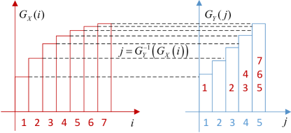
(a) Mapping 1

(b) Mapping 2

Figure 1: Illustrations of Mappings 1 and 2.

II Rényi Distribution Approximation

II-A Asymptotics of Rényi Divergences

We first characterize the asymptotics of Rényi divergences $D_{\alpha}(P_{Y^{n}}\|Q_{Y}^{n})$, $D_{\alpha}(Q_{Y}^{n}\|P_{Y^{n}})$, and $D_{\alpha}^{\mathsf{max}}(P_{Y^{n}},Q_{Y}^{n})$, as shown by the following theorems.

Theorem 1 (Asymptotics of $\frac{1}{n}D_{\alpha}(P_{Y^{n}}\|Q_{Y}^{n})$).

For any $\alpha\in[0,\infty]$, we have

$$\lim_{n\to\infty}\frac{1}{n}\inf_{f}D_{\alpha}(P_{Y^{n}}\|Q_{Y}^{n})$$

$$=\sup_{t\in[0,1)}\left\{tH_{\frac{1}{1-t}}(Q_{Y})-\frac{t}{R}H_{\frac{1}{1-\frac{\alpha-1}{\alpha}t}}(P_{X})\right\}.$$ (25)

Theorem 2 (Asymptotics of $\frac{1}{n}D_{\alpha}(Q_{Y}^{n}\|P_{Y^{n}})$).

For any $\alpha\in[0,\infty]$, we have

$$\lim_{n\to\infty}\frac{1}{n}\inf_{f}D_{\alpha}(Q_{Y}^{n}\|P_{Y^{n}})$$

$$=\begin{cases}\infty,\quad\alpha\in[1,\infty]\textrm{ and }R>\frac{H_{0}(P_{X})}{H_{0}(Q_{Y})};\\ \sup_{t\in(0,\infty)}\left\{tH_{\frac{1}{1+\frac{\alpha-1}{\alpha}t}}(Q_{Y})-\frac{t}{R}H_{\frac{1}{1+t}}(P_{X})\right\},\\ \qquad\;\alpha\in[1,\infty]\textrm{ and }R<\frac{H_{0}(P_{X})}{H_{0}(Q_{Y})};\\ \frac{\alpha}{1-\alpha}\max_{t\in[0,1]}\left\{tH_{\frac{1}{1-t}}(Q_{Y})-\frac{t}{R}H_{\frac{1}{1+\frac{\alpha}{1-\alpha}t}}(P_{X})\right\},\\ \qquad\;\alpha\in(0,1);\\ 0,\quad\;\alpha=0.\end{cases}$$ (26)

Theorem 3 (Asymptotics of $\frac{1}{n}D_{\alpha}^{\mathsf{max}}(P_{Y^{n}},Q_{Y}^{n})$).

For any $\alpha\in[0,\infty]$, we have (27) (given on page 27),

$$\lim_{n\to\infty}\frac{1}{n}\inf_{f}D_{\alpha}^{\mathsf{max}}(P_{Y^{n}},Q_{Y}^{n})$$

$$=\begin{cases}\infty,&\alpha\in[1,\infty]\textrm{ and }R>\frac{H_{0}(P_{X})}{H_{0}(Q_{Y})}\\ \max\biggl{\{}\sup_{t\in[0,1)\cup(\frac{\alpha}{\alpha-1},\infty)}\left\{tH_{\frac{1}{1-t}}(Q_{Y})-\frac{t}{R}H_{\frac{1}{1-\frac{\alpha-1}{\alpha}t}}(P_{X})\right\},\\ \qquad\sup_{t\in(0,\infty)}\left\{tH_{\frac{1}{1+\frac{\alpha-1}{\alpha}t}}(Q_{Y})-\frac{t}{R}H_{\frac{1}{1+t}}(P_{X})\right\}\biggr{\}},&\alpha\in(1,\infty]\textrm{ and }R<\frac{H_{0}(P_{X})}{H_{0}(Q_{Y})}\\ \max\biggl{\{}\sup_{t\in[0,1)}\left\{tH_{\frac{1}{1-t}}(Q_{Y})-\frac{t}{R}H(P_{X})\right\},\\ \qquad\sup_{t\in(0,\infty)}\left\{tH(Q_{Y})-\frac{t}{R}H_{\frac{1}{1+t}}(P_{X})\right\}\biggr{\}},&\alpha=1\textrm{ and }R<\frac{H_{0}(P_{X})}{H_{0}(Q_{Y})}\\ \sup_{t\in[0,1)}\max_{t^{\prime}\in[0,1]}\left\{tb(t^{\prime})H_{\frac{1}{1-t}}(Q_{Y})-\frac{tb(t^{\prime})}{R}H_{\frac{1}{1+\frac{b(t^{\prime})}{a(t^{\prime})}t}}(P_{X})\right\},&\alpha\in(0,1)\\ \sup_{t\in[0,1)}\left\{tH_{\frac{1}{1-t}}(Q_{Y})-\frac{t}{R}H_{0}(P_{X})\right\},&\alpha=0\end{cases}$$ (27)

where

$$a(t^{\prime}) =\left(\frac{\alpha}{1-\alpha}-1\right)t^{\prime}+1$$ (28)

$$b(t^{\prime}) =\left(1-\frac{\alpha}{1-\alpha}\right)t^{\prime}+\frac{\alpha}{1-\alpha}.$$ (29)

Remark 1.

For $\alpha\in[1,\infty]$ and $R=\frac{H_{0}(P_{X})}{H_{0}(Q_{Y})}$, the asymptotic behavior of $\frac{1}{n}\inf_{f}D_{\alpha}(Q_{Y}^{n}\|P_{Y^{n}})$ and $\frac{1}{n}\inf_{f}D_{\alpha}^{\mathsf{max}}(P_{Y^{n}},Q_{Y}^{n})$ depends on how fast $\frac{n}{k}$ converges to $R$. In this paper, we set $n=\left\lceil kR\right\rceil$, i.e., the fastest case. For this case, $\frac{1}{n}\inf_{f}D_{\alpha}(Q_{Y}^{n}\|P_{Y^{n}})=\frac{1}{n}\inf_{f}D_{\alpha}^{\mathsf{max}}(P_{Y^{n}},Q_{Y}^{n})=\infty$, if $kR\notin\mathbb{N}$; and $\frac{1}{n}\inf_{f}D_{\alpha}(Q_{Y}^{n}\|P_{Y^{n}})=\frac{1}{n}D_{\alpha}(\{Q_{i}\}\|\{P_{i}\})$ and $\frac{1}{n}\inf_{f}D_{\alpha}^{\mathsf{max}}(P_{Y^{n}},Q_{Y}^{n})=\frac{1}{n}\max\left\{D_{\alpha}(\{P_{i}\}\|\{Q_{i}\}),D_{\alpha}(\{Q_{i}\}\|\{P_{i}\})\right\}$, if $kR\in\mathbb{N}$, where $\{P_{i}\}$ and $\{Q_{i}\}$ respectively denote the resulting sequences after sorting the elements of $P_{X}^{k}$ and $Q_{Y}^{n}$ in descending order.

The proofs of Theorems 1, 2, and 3 are provided in Appendices B, C, and D, respectively. For the achievability parts, we partition the sequences in $\mathcal{X}^{k}$ and $\mathcal{Y}^{n}$ into type classes, and design codes on the level of type classes. More specifically, for Theorem 1, we first design a function $g:\mathcal{P}^{\left(k\right)}\left(\mathcal{X}\right)\to\mathcal{P}^{\left(n\right)}\left(\mathcal{Y}\right)$ that maps $k$-types on $\mathcal{X}$ to $n$-types on $\mathcal{Y}$; and then a code $f$ induced by $g$ is obtained by mapping the sequences in $\mathcal{T}_{T_{X}}$ to the sequences in $\mathcal{T}_{g(T_{X})}$ as uniformly as possible for all $T_{X}\in\mathcal{P}^{\left(k\right)}\left(\mathcal{X}\right)$, i.e., $f$ maps approximately $\nicefrac{{\left|\mathcal{T}_{T_{X}}\right|}}{{\left|\mathcal{T}_{g(T_{X})}\right|}}$ sequences in $\mathcal{T}_{T_{X}}$ to each distinct sequence in $\mathcal{T}_{g(T_{X})}$. Here the optimal selection of the function $g$ depends on $s$ and requires careful analysis (the detail can be found in the proof). The intuition of designing such a code is given in the following. On one hand, observe that

$$\frac{1}{n}D_{1+s}(P_{Y^{n}}\|Q_{Y}^{n})$$

$$=\frac{1}{ns}\log\biggl{\{}\sum_{T_{Y}}\sum_{y^{n}\in\mathcal{T}_{T_{Y}}}$$

$$\quad\Bigl{(}\sum_{T_{X}}\sum_{x^{k}\in\mathcal{T}_{T_{X}}}P_{X}^{k}(x^{k})1\left\{y^{n}=f(x^{k})\right\}\Bigr{)}^{1+s}Q_{Y}^{n}(y^{n})^{-s}\biggr{\}}$$ (30)

$$=\frac{1}{ns}\log\biggl{\{}\max_{T_{X},T_{Y}}\sum_{y^{n}\in\mathcal{T}_{T_{Y}}}$$

$$\quad\Bigl{(}\sum_{x^{k}\in\mathcal{T}_{T_{X}}}P_{X}^{k}(x^{k})1\left\{y^{n}=f(x^{k})\right\}\Bigr{)}^{1+s}Q_{Y}^{n}(y^{n})^{-s}\biggr{\}}+o(1)$$ (31)

where (31) follows since the number of $n$-types (or $k$-types) is only polynomial in $n$ (or $k$). This means that for any code $f$, the asymptotics of $\frac{1}{n}D_{1+s}(P_{Y^{n}}\|Q_{Y}^{n})$ induced by $f$ is only determined by restrictions of $f$ on $\mathcal{A}\left(T_{X},T_{Y}\right):=\left\{x^{n}\in\mathcal{T}_{T_{X}}:\>f(x^{n})\in\mathcal{T}_{T_{Y}}\right\}$ for different $\left(T_{X},T_{Y}\right)$. In other words, the performance of a code $f$ only depends on its restrictions to those maps from $\mathcal{A}\left(T_{X},T_{Y}\right)$ to $\mathcal{T}_{T_{Y}}$. On the other hand, $P_{X}^{k}(x^{k})$ and $Q_{Y}^{n}(y^{n})$ are uniform on $\mathcal{T}_{T_{X}}$ and $\mathcal{T}_{T_{Y}}$, respectively. Hence for different $\left(T_{X},T_{Y}\right)$, to make the objective function of (31) as small as possible, we need to map the sequences in $\mathcal{A}\left(T_{X},T_{Y}\right)$ to the sequences in $\mathcal{T}_{T_{Y}}$ as uniformly as possible. Since $\bigcup_{T_{Y}}\mathcal{A}\left(T_{X},T_{Y}\right)=\mathcal{T}_{T_{X}}$ and the number of types $T_{Y}$ is polynomial in $n$, for each $T_{X}$, there is a dominant type $T_{Y}=g(T_{X})$ such that redefining $f$ to satisfy $\left\{f(x^{n}),x^{n}\in\mathcal{T}_{T_{X}}\right\}\subseteq\mathcal{T}_{T_{Y}}$ with $T_{Y}=g(T_{X})$ does not affect the asymptotics of $\frac{1}{n}D_{1+s}(P_{Y^{n}}\|Q_{Y}^{n})$. Therefore, we only need to consider the codes consisting of a function $g$ that maps $k$-types on $\mathcal{X}$ to $n$-types on $\mathcal{Y}$, and mappings that map sequences in $\mathcal{T}_{T_{X}}$ to sequences in $\mathcal{T}_{g(T_{X})}$ as uniformly as possible.

The achievability proof for Theorem 2 follows similar ideas. However, in contrast, to ensure that $\frac{1}{n}\inf_{f}D_{\alpha}(Q_{Y}^{n}\|P_{Y^{n}})$ is finite and also as small as possible, it is required that $\operatorname{supp}\left(P_{Y^{n}}\right)\supseteq\operatorname{supp}\left(Q_{Y}^{n}\right)$ and $P_{Y^{n}}(y^{n})$ should be as large as possible for all $y^{n}$. On the other hand, observe that $\left|\mathcal{P}^{\left(n\right)}\left(\mathcal{Y}\right)\right|$ is polynomial in $n$. Hence for each $T_{X}$, we should partition $\mathcal{T}_{T_{X}}$ into $\left|\mathcal{P}^{\left(n\right)}\left(\mathcal{Y}\right)\right|$ subsets with equal size, and for each $T_{Y}$, map the sequences in each subset to the sequences in the set $\mathcal{T}_{T_{Y}}$ as uniformly as possible. Observe that for each $T_{Y}$, there must exist a type $T_{X}$ such that $H(T_{X})\geq H(T_{Y})+o(1)$ (otherwise $\frac{1}{n}\inf_{f}D_{\alpha}(Q_{Y}^{n}\|P_{Y^{n}})=\infty$) and moreover, similar to (31), the summation term is dominated by some type $T_{X}$ such that $H(T_{X})\geq H(T_{Y})+o(1)$. Hence without loss of any optimality, it suffices to consider the following mapping. For each $T_{X}$ and $\delta>0$, partition $\mathcal{T}_{T_{X}}$ into $\left|\left\{T_{Y}:H(T_{X})\geq H(T_{Y})+\delta\right\}\right|$ subsets with approximately same size. For each $T_{Y}$ such that $H(T_{X})\geq H(T_{Y})+\delta$, map the sequences in each subset to the sequences in the set $\mathcal{T}_{T_{Y}}$ as uniformly as possible.

The code used to prove the achievability part of Theorem 3 is a combination of the two codes above.

II-B Rényi Conversion Rates

As shown in the theorems above, when the code rate is large, the normalized Rényi divergences $\frac{1}{n}D_{\alpha}(P_{Y^{n}}\|Q_{Y}^{n})$, $\frac{1}{n}D_{\alpha}(Q_{Y}^{n}\|P_{Y^{n}})$, and $\frac{1}{n}D_{\alpha}^{\mathsf{max}}(P_{Y^{n}},Q_{Y}^{n})$ converge to a positive number; however when the code rate is small enough, the normalized Rényi divergences converge to zero. This threshold rate, termed the Rényi conversion rate, is important, since it represents the maximum possible rate under the condition that the distribution induced by the code approximates the target distribution arbitrarily well as $n\to\infty$. We characterize the Rényi conversion rates for normalized and unnormalized $D_{\alpha}(P_{Y^{n}}\|Q_{Y}^{n})$, $D_{\alpha}(Q_{Y}^{n}\|P_{Y^{n}})$, and $D_{\alpha}^{\mathsf{max}}(P_{Y^{n}},Q_{Y}^{n})$ in the following theorems.

Theorem 4 (Rényi Conversion Rate for $D_{\alpha}(P_{Y^{n}}\|Q_{Y}^{n})$).

For any $\alpha\in[0,\infty]$,

$$\sup\left\{R:\frac{1}{n}D_{\alpha}(P_{Y^{n}}\|Q_{Y}^{n})\rightarrow 0\right\}$$

$$=\begin{cases}\inf_{t\in(0,1)}\frac{H_{\frac{1}{1-\frac{\alpha-1}{\alpha}t}}(P_{X})}{H_{\frac{1}{1-t}}(Q_{Y})},&\alpha\in[1,\infty]\\ \frac{H(P_{X})}{H(Q_{Y})},&\alpha\in(0,1)\\ \frac{H_{0}(P_{X})}{H(Q_{Y})},&\alpha=0\end{cases}.$$ (32)

For $\alpha\in[0,1]\cup\left\{\infty\right\}$, we have

$$\sup\left\{R:D_{\alpha}(P_{Y^{n}}\|Q_{Y}^{n})\rightarrow 0\right\}$$

$$=\sup\left\{R:\frac{1}{n}D_{\alpha}(P_{Y^{n}}\|Q_{Y}^{n})\rightarrow 0\right\}.$$ (33)

For $\alpha\in[1,\infty]$, we have

$$\sup\left\{R:\frac{1}{n}D_{\alpha}(P_{Y^{n}}\|Q_{Y}^{n})\rightarrow 0\right\}$$

$$\geq\sup\left\{R:D_{\alpha}(P_{Y^{n}}\|Q_{Y}^{n})\rightarrow 0\right\}$$ (34)

$$\geq\inf_{t\in(0,1)}\frac{H_{\frac{\alpha-1+t}{\alpha-1+t-\left(\alpha-1\right)t}}(P_{X})}{H_{\frac{1}{1-t}}(Q_{Y})}.$$ (35)

Remark 2.

The analogous result under the TV distance measure was first shown by Han [1]. Theorem 4 is an extension of [1] to the Rényi divergence of all orders $\alpha\in[0,\infty]$. Besides, the first-order and second-order rates, as well as the conversion rates of the quantum version, for the unnormalized Rényi divergence $D_{\alpha}(P_{Y^{n}}\|Q_{Y}^{n})$ with $\alpha=\frac{1}{2}$ were given by Kumagai and Hayashi [2]; and the corresponding moderate deviation of the quantum Rényi conversion rates with the same order was studied by Chubb, Tomamichel, and Korzekwa1 [14]. The result for the unnormalized Rényi divergence with $\alpha\in(0,\frac{1}{2})$ can be obtained by combining two observations: 1) the achievability for $D_{\frac{1}{2}}(P_{Y^{n}}\|Q_{Y}^{n})$ implies the achievability for $\alpha\in(0,\frac{1}{2})$; 2) by Pinsker’s inequality for Rényi divergence [3], the converse result for the TV distance measure [1] implies the converse for $\alpha\in(0,\frac{1}{2})$. Our results for orders $\alpha\in\left\{0\right\}\cup(\frac{1}{2},\infty]$ are new.

Remark 3.

$D_{\alpha}(P_{Y|X=x}\|P_{Y|X=x^{\prime}})\leq\epsilon$ for all neighboring databases $x,x^{\prime}$ is known as the $\epsilon$-Rényi differential privacy of order $\alpha$ [15], and the special case with $\alpha=\infty$ is known as the $\epsilon$-differential privacy [16]. Here, $X$ represents public data and $Y$ represents private data. In the theorem above, this measure is applied to the random variable simulation problem, and we provide a “necessary and sufficient condition” for $\lim_{n\to\infty}\frac{1}{n}D_{\alpha}\leq\epsilon$ for any $\epsilon>0$.

Theorem 5 (Rényi Conversion Rate for $D_{\alpha}(Q_{Y}^{n}\|P_{Y^{n}})$).

For any $\alpha\in[0,\infty]$,

$$\sup\left\{R:\frac{1}{n}D_{\alpha}(Q_{Y}^{n}\|P_{Y^{n}})\rightarrow 0\right\}$$

$$=\begin{cases}\inf_{t\in(0,\infty)}\frac{H_{\frac{1}{1+t}}(P_{X})}{H_{\frac{1}{1+\frac{\alpha-1}{\alpha}t}}(Q_{Y})},&\alpha\in(1,\infty]\\ \min\left\{\frac{H(P_{X})}{H(Q_{Y})},\frac{H_{0}(P_{X})}{H_{0}(Q_{Y})}\right\},&\alpha=1\\ \frac{H(P_{X})}{H(Q_{Y})},&\alpha\in(0,1)\\ \infty,&\alpha=0\end{cases}.$$ (36)

For $\alpha\in[0,1]\cup\left\{\infty\right\}$, we have

$$\sup\left\{R:D_{\alpha}(Q_{Y}^{n}\|P_{Y^{n}})\rightarrow 0\right\}$$

$$=\sup\left\{R:\frac{1}{n}D_{\alpha}(Q_{Y}^{n}\|P_{Y^{n}})\rightarrow 0\right\}.$$ (37)

Remark 4.

Our results for all orders $\alpha\in[0,\infty]$ are new.

Theorem 6 (Rényi Conversion Rate for $D_{\alpha}^{\mathsf{max}}(P_{Y^{n}},Q_{Y}^{n})$).

For $\alpha\in[0,\infty]$, we have

$$\sup\left\{R:\frac{1}{n}D_{\alpha}^{\mathsf{max}}(P_{Y^{n}},Q_{Y}^{n})\rightarrow 0\right\}$$

$$=\begin{cases}\min\Biggl{\{}\inf_{t\in[0,1)\cup(\frac{\alpha}{\alpha-1},\infty)}\frac{H_{\frac{1}{1-\frac{\alpha-1}{\alpha}t}}(P_{X})}{H_{\frac{1}{1-t}}(Q_{Y})},\\ \qquad\inf_{t\in(0,\infty)}\frac{H_{\frac{1}{1+t}}(P_{X})}{H_{\frac{1}{1+\frac{\alpha-1}{\alpha}t}}(Q_{Y})}\Biggr{\}},&\alpha\in(1,\infty]\\ \min\left\{\frac{H(P_{X})}{H(Q_{Y})},\frac{H_{0}(P_{X})}{H_{0}(Q_{Y})}\right\},&\alpha=1\\ \frac{H(P_{X})}{H(Q_{Y})},&\alpha\in(0,1)\\ \frac{H_{0}(P_{X})}{H(Q_{Y})},&\alpha=0\end{cases}.$$ (38)

For $\alpha\in[0,1]\cup\left\{\infty\right\}$, we have

$$\sup\left\{R:D_{\alpha}^{\mathsf{max}}(P_{Y^{n}},Q_{Y}^{n})\rightarrow 0\right\}$$

$$=\sup\left\{R:\frac{1}{n}D_{\alpha}^{\mathsf{max}}(P_{Y^{n}},Q_{Y}^{n})\rightarrow 0\right\}.$$ (39)

Remark 5.

Note that for $\alpha\in(1,\infty]$, (38) involves an infimum taken over $(\frac{\alpha}{\alpha-1},\infty)$, and hence it is in general smaller than the minimum of (32) and (36).

Remark 6.

For $\alpha=\infty$, the Rényi conversion rate in (38) is $\min_{\beta\in[-\infty,\infty]}\frac{H_{\beta}(P_{X})}{H_{\beta}(Q_{Y})}$. Consider $R=1$. Then this theorem implies that $P_{X}^{n}$ can approximate $Q_{Y}^{n}$ in the sense that $\frac{1}{n}D_{\infty}^{\mathsf{max}}(P_{Y^{n}},Q_{Y}^{n})\rightarrow 0$ or $D_{\infty}^{\mathsf{max}}(P_{Y^{n}},Q_{Y}^{n})\rightarrow 0$, if $H_{\beta}(P_{X})>H_{\beta}(Q_{Y})$ for all $\beta\in[-\infty,\infty]$, and only if $H_{\beta}(P_{X})\geq H_{\beta}(Q_{Y})$ for all $\beta\in[-\infty,\infty]$. This also implies the statement 1) of [17, Proposition III.3], since if $H_{\beta}(P_{X})<H_{\beta}(Q_{Y})$ for some $\beta\in[-\infty,\infty]$, then approximate simulation (under the measure $D_{\infty}^{\mathsf{max}}$) is impossible, and hence exact simulation is also impossible.

Remark 7.

Note that $D_{\infty}^{\mathsf{max}}$ is an extremely strong distance measure. Theorem 6 states that the Rényi conversion rate (the maximum possible rate under the condition $D_{\infty}^{\mathsf{max}}(P_{Y^{n}},Q_{Y}^{n})\rightarrow 0$) is finite. That is to say, as the dimension tends to infinity, it is always possible to achieve $D_{\infty}^{\mathsf{max}}(P_{Y^{n}},Q_{Y}^{n})\rightarrow 0$, even though $D_{\infty}^{\mathsf{max}}$ is extremely strong. However, in our recent work [17, Proposition III.4], we showed that for some special pairs of distributions, it is impossible to achieve $P_{Y^{n}}=Q_{Y}^{n}$ (or $D_{\infty}^{\mathsf{max}}(P_{Y^{n}},Q_{Y}^{n})=0$) for finite $n$, i.e, the exact simulation cannot be obtained for finite-dimensional product of distributions. Hence there exists a big “gap” between approximate simulation and exact simulation (for fixed blocklength cases), even when the approximate simulation is realized under the measure $D_{\infty}^{\mathsf{max}}$.

Remark 8.

The condition $D_{\infty}^{\mathsf{max}}(P,Q)\leq\epsilon$ is called $\left(\epsilon,0\right)$-closeness, and was used to measure privacy in [13]. In Theorem 6, we provide a “necessary and sufficient condition” for $\lim_{n\to\infty}D_{\infty}^{\mathsf{max}}(P_{Y^{n}},Q_{Y}^{n})\leq\epsilon$ or $\lim_{n\to\infty}\frac{1}{n}D_{\infty}^{\mathsf{max}}(P_{Y^{n}},Q_{Y}^{n})\leq\epsilon$ for any $\epsilon>0$. $D_{\infty}^{\mathsf{max}}(P,Q)$ is a very strong measure, hence it can be taken as a secrecy measure for a secrecy system when secrecy stronger than the usual notion of strong secrecy is required. Our result can be applied to this case. Furthermore, $D_{\infty}^{\mathsf{max}}(P,Q)$ is also related to $\epsilon$-information privacy, which is defined as $D_{\infty}^{\mathsf{max}}(P_{XY},P_{X}P_{Y})\leq\epsilon$ where $X$ and $Y$ represent public and private datum respectively [18].

The proofs of Theorems 4, 5, and 6 are provided in Appendices E, F, and G, respectively. The Rényi conversion rates for normalized $D_{\alpha}(P_{Y^{n}}\|Q_{Y}^{n})$, $D_{\alpha}(Q_{Y}^{n}\|P_{Y^{n}})$, and $D_{\alpha}^{\mathsf{max}}(P_{Y^{n}},Q_{Y}^{n})$ respectively follow from Theorems 1, 2, and 3. Obviously, the unnormalized Rényi conversion rates are lower bounded by the normalized ones. We believe such lower bounds are tight. However, we do not know how to construct an efficient coding scheme for the case $\alpha\in(1,\infty)$. Hence for the measure $D_{\alpha}(P_{Y^{n}}\|Q_{Y}^{n})$, we consider a relatively simple scheme — the inverse-transform scheme, which is described in Subsection I-E and illustrated in Fig. 1a. Another reason for using the inverse-transform scheme is that such a scheme is optimal (which results in zero divergences) when the source distribution $P_{X}$ is continuous [19, Proposition 1]. Hence we believe it should work also well for discrete source distributions. The specific code used to prove the achievability part for this case is illustrated in Fig. 6. For $\delta>0$, define $\mathcal{B}_{1}:=\left\{y^{n}:Q_{Y}^{n}(y^{n})\geq e^{-n\left(H(Q_{Y})+\delta\right)}\right\}$. To ensure $D_{\alpha}(P_{Y^{n}}\|Q_{Y}^{n})\to 0$, we only need to simulate a truncated version $\widetilde{Q}_{Y^{n}}(y^{n}):=\frac{Q_{Y}^{n}(y^{n})}{Q_{Y}^{n}(\mathcal{B}_{1})}1\left\{y^{n}\in\mathcal{B}_{1}\right\}$ of $Q_{Y}^{n}$. This is because, on one hand, for any function $f:\mathcal{X}^{k}\to\mathcal{B}_{1}$ with output $Y^{n}=f(X^{k})$,

$$D_{\alpha}(P_{Y^{n}}\|Q_{Y}^{n})$$

$$=\frac{1}{\alpha-1}\log\sum_{y^{n}\in\mathcal{A}}P_{Y^{n}}(y^{n})\left(\frac{P_{Y^{n}}(y^{n})}{\widetilde{Q}_{Y^{n}}(y^{n})}\frac{\widetilde{Q}_{Y^{n}}(y^{n})}{Q_{Y}^{n}(y^{n})}\right)^{\alpha-1}$$ (40)

$$=\frac{1}{\alpha-1}\log\sum_{y^{n}\in\mathcal{A}}P_{Y^{n}}(y^{n})\left(\frac{P_{Y^{n}}(y^{n})}{\widetilde{Q}_{Y^{n}}(y^{n})}\frac{1}{Q_{Y}^{n}(\mathcal{B}_{1})}\right)^{\alpha-1}$$ (41)

$$=D_{\alpha}(P_{Y^{n}}\|\widetilde{Q}_{Y^{n}})-\log Q_{Y}^{n}(\mathcal{B}_{1}),$$ (42)

and on the other hand, observe that $Q_{Y}^{n}(\mathcal{B}_{1})\to 1$ as $n\to\infty$. That is to say, if a function $f$ is a “good” simulator for $\widetilde{Q}_{Y^{n}}$ in the sense that $D_{\alpha}(P_{Y^{n}}\|\widetilde{Q}_{Y^{n}})\to 0$, then it must be also “good” for $Q_{Y}^{n}$ in the same sense. The reason why we consider simulating $\widetilde{Q}_{Y^{n}}$ rather than simulating $Q_{Y}^{n}$ directly, is that by doing this, the influence of the behavior of $\left\{Q_{Y}^{n}(y^{n}):y^{n}\in\mathcal{Y}^{n}\backslash\mathcal{B}_{1}\right\}$ on the value of $D_{\alpha}(P_{Y^{n}}\|Q_{Y}^{n})$ is removed, since for such a simulation, all sequences $x^{n}$ are mapped to the sequences $y^{n}$ in $\mathcal{B}_{1}$. Hence in general, a code $f:\mathcal{X}^{k}\to\mathcal{B}_{1}$ induces a smaller $D_{\alpha}(P_{Y^{n}}\|Q_{Y}^{n})$ than a code $f:\mathcal{X}^{k}\to\mathcal{Y}^{n}$. By using the inverse-transform scheme, we derive an upper bound for $\alpha\in[1,\infty]$, which is tight for $\alpha=1$ or $\infty$. This is because that to ensure $D_{\alpha}(P_{Y^{n}}\|Q_{Y}^{n})\to 0$, it is required that $\frac{P_{Y^{n}}(y^{n})}{Q_{Y}^{n}(y^{n})}\leq 1+o(1)$ for all $y^{n}\in\mathcal{Y}^{n}$ when $\alpha=\infty$, and $\frac{P_{Y^{n}}(y^{n})}{Q_{Y}^{n}(y^{n})}=1+o(1)$ for all $y^{n}$ in a high probability set of $Q_{Y}^{n}$ when $\alpha=1$.

Similar ideas also apply to the cases with measures $D_{\alpha}(Q_{Y}^{n}\|P_{Y^{n}})$ and $D_{\alpha}^{\mathsf{max}}(P_{Y^{n}},Q_{Y}^{n})$. However, for $\alpha=1$, differently from the case $D_{\alpha}(P_{Y^{n}}\|Q_{Y}^{n})$, to ensure $D_{\alpha}(Q_{Y}^{n}\|P_{Y^{n}})\to 0$ or $D_{\alpha}^{\mathsf{max}}(P_{Y^{n}},Q_{Y}^{n})\to 0$, it is required not only that $\frac{Q_{Y}^{n}(y^{n})}{P_{Y^{n}}(y^{n})}=1+o(1)$ for all $y^{n}$ in a high probability set of $Q_{Y}^{n}$, but also that $P_{Y^{n}}(y^{n})>0$ for all $y^{n}\in\mathcal{Y}^{n}$ (otherwise, $D_{\alpha}(Q_{Y}^{n}\|P_{Y^{n}})=D_{\alpha}^{\mathsf{max}}(P_{Y^{n}},Q_{Y}^{n})=\infty$). Observe that there exists a code such that $P_{Y^{n}}(y^{n})>0$ for all $y^{n}\in\mathcal{Y}^{n}$ if and only if $|\mathcal{X}|^{k}\geq|\mathcal{Y}|^{n}$, i.e., $\frac{n}{k}\leq\frac{H_{0}(P_{X})}{H_{0}(Q_{Y})}$. Hence the term $\frac{H_{0}(P_{X})}{H_{0}(Q_{Y})}$ appears in (36) and (38) for $\alpha=1$.

For $\alpha=\infty$ and for the measure $D_{\alpha}(Q_{Y}^{n}\|P_{Y^{n}})$, the code used to prove the achievability part is illustrated in Fig. 7. In contrast to the case $D_{\alpha}(P_{Y^{n}}\|Q_{Y}^{n})$, here the sequences in $\mathcal{B}_{2}:=\left\{y^{n}:e^{-nH^{\mathrm{u}}(Q_{Y})}\leq Q_{Y}^{n}(y^{n})\leq e^{-n\left(H(Q_{Y})-\delta\right)}\right\}$, instead of those in $\mathcal{B}_{1}$, are dominant. That is to say, the influence of $\{Q_{Y}^{n}(y^{n}):y^{n}\in\mathcal{Y}^{n}\backslash\mathcal{B}_{2}\}$ on the value of $D_{\alpha}(Q_{Y}^{n}\|P_{Y^{n}})$ can be removed. However, for the measure $D_{\alpha}^{\mathsf{max}}(P_{Y^{n}},Q_{Y}^{n})$, the influence of $Q_{Y}^{n}(y^{n}),y^{n}\in\mathcal{Y}^{n}$ cannot be removed anymore. That is, all the sequences in $\mathcal{Y}^{n}$ are dominant. See the code illustrated in Fig. 8, which is used to prove the achievability part for this case.

In summary, for $\alpha=\infty$, the conversion rates are determined by the (part of or all of) information spectrum exponents of $P_{X}^{k}$ and $Q_{Y}^{n}$, and on the other hand, the information spectrum exponents are determined by the Rényi entropies (see Lemmas 9 and 11; more specifically, the infinity order cases in Theorems 4, 5, and 6 respectively correspond to (101), (103), as well as, (101) and (102)). Hence the conversion rates are determined by Rényi entropies. This is the reason why the conversion rates are expressed as functions of Rényi entropies. However, for $\alpha=1$, the conversion rates are related to the limits of information spectrums of $P_{X}^{k}$ and $Q_{Y}^{n}$, and do not depend on how fast the information spectrums converge. Hence they are only functions of Rényi entropies with orders 1 and 0.

Theorems 4, 5, and 6 are illustrated in Fig. 2.

Figure 2: Illustration of the Rényi conversion rates under normalized divergences in Theorems 4, 5, and 6 for $P_{X}=\mathsf{Bern}\left(0.3\right)$ and $Q_{Y}=\mathsf{Bern}\left(0.1\right)$ (top) and for $P_{X}=\mathsf{Bern}\left(0.1\right)$ and $Q_{Y}=\mathsf{Bern}\left(0.3\right)$ (bottom).

III Special Case 1: Rényi Source Resolvability

If we set $P_{X}$ to the Bernoulli distribution $\mathsf{Bern}(\frac{1}{2})$, then the distribution approximation problem reduces to the source resolvability problem, i.e., simulating a memoryless source whose distribution is approximately subject to a target distribution $Q_{Y}$, using a uniform random variable $M_{n}$ that is uniformly distributed over $\mathcal{M}_{n}:=[1:\mathsf{M}]$ with $\mathsf{M}:=\lfloor e^{n\widetilde{R}}\rfloor$. The rate $\widetilde{R}$ here is different from the $R$ defined in Section II, and indeed it is approximately equal to the ratio of $\log 2$ and the $R$ in Section II with $P_{X}$ set to $\mathsf{Bern}(\frac{1}{2})$. Given the target distribution $Q_{Y}$, we wish to minimize the rate $\widetilde{R}$ such that the distribution of $Y^{n}:=f(M_{n})$ forms a good approximation to the product distribution $Q_{Y}^{n}$. In contrast to previous works on the resolvability problem [4, 8], here we employ the Rényi divergences $D_{\alpha}(P_{Y^{n}}\|Q_{Y}^{n}),D_{\alpha}(Q_{Y}^{n}\|P_{Y^{n}})$, and $D_{\alpha}^{\mathsf{max}}(P_{Y^{n}},Q_{Y}^{n})$ of all orders $\alpha\in[0,\infty]$ to measure the discrepancy between $P_{Y^{n}}$ and $Q_{Y}^{n}$.

III-A Asymptotics of Rényi Divergences

We consider the Rényi divergences $D_{\alpha}(P_{Y^{n}}\|Q_{Y}^{n}),D_{\alpha}(Q_{Y}^{n}\|P_{Y^{n}})$, and $D_{\alpha}^{\mathsf{max}}(P_{Y^{n}},Q_{Y}^{n})$. The asymptotic behaviors of these measures are respectively characterized in the following corollaries. These results follow from Theorems 1, 2, and 3 by setting $P_{X}=\mathsf{Bern}(\frac{1}{2})$.

Corollary 1 (Asymptotics of $\frac{1}{n}D_{\alpha}(P_{Y^{n}}\|Q_{Y}^{n})$).

For any $\alpha\in[0,\infty]$, we have

$$\lim_{n\to\infty}\frac{1}{n}\inf_{f}D_{\alpha}(P_{Y^{n}}\|Q_{Y}^{n})$$

$$=\sup_{t\in[0,1)}\left\{tH_{\frac{1}{1-t}}(Q_{Y})-t\widetilde{R}\right\}.$$ (43)

Remark 9.

This result for $\alpha\in[0,2]$ was shown by our previous work [8]. Hence our results here for $\alpha\in(2,\infty]$ are new.

Remark 10.

This result for $\alpha=0$ is related to the error exponent of lossless source coding. Define

$$\mathsf{P}\left(\widetilde{R}\right):=\sup_{\mathcal{A}\subseteq\mathcal{Y}:|\mathcal{A}|\leq e^{n\widetilde{R}}}Q_{Y}^{n}\left(\mathcal{A}\right).$$ (44)

Then according to (14), for $\alpha=0$, the asymptotics of the normalized Rényi divergence

$$\lim_{n\to\infty}\frac{1}{n}\inf_{f}D_{0}(P_{Y^{n}}\|Q_{Y}^{n})$$

$$=\lim_{n\to\infty}-\frac{1}{n}\log\mathsf{P}\left(\widetilde{R}\right)$$ (45)

$$=\min_{\widetilde{P}_{Y}:H(\widetilde{P}_{Y})\leq\widetilde{R}}D(\widetilde{P}_{Y}\|Q_{Y})$$ (46)

$$=\sup_{t\in[0,1)}\left\{tH_{\frac{1}{1-t}}(Q_{Y})-t\widetilde{R}\right\}.$$ (47)

On the other hand, the error exponent of lossless source coding with code rate $\widetilde{R}$ for memoryless source $Q_{Y}^{n}$ is

$$\lim_{n\to\infty}-\frac{1}{n}\log\left(1-\mathsf{P}\left(\widetilde{R}\right)\right)$$

$$=\min_{\widetilde{P}_{Y}:H(\widetilde{P}_{Y})\geq\widetilde{R}}D(\widetilde{P}_{Y}\|Q_{Y})$$ (48)

$$=\sup_{t\in[0,\infty)}\left\{-tH_{\frac{1}{1+t}}(Q_{Y})+t\widetilde{R}\right\}.$$ (49)

Hence the asymptotics of the normalized Rényi divergence $D_{0}(P_{Y^{n}}\|Q_{Y}^{n})$ and the error exponent of lossless source coding are respectively the exponents of $\mathsf{P}\left(\widetilde{R}\right)$ for different regimes ($\widetilde{R}\leq H(Q_{Y})$ and $\widetilde{R}\geq H(Q_{Y})$). Furthermore, by large deviation theory [27], (44)-(49) hold not only for finite alphabets, but also for countably infinite or continuous alphabets (with the counting measure replaced by the Lebesgue measure, the probability mass function $Q_{Y}$ replaced by the corresponding probability density function or the Radon-Nikodym derivative, and the summation replaced by the corresponding integration).

Corollary 2 (Asymptotics of $\frac{1}{n}D_{\alpha}(Q_{Y}^{n}\|P_{Y^{n}})$).

For any $\alpha\in[0,\infty]$, we have

$$\lim_{n\to\infty}\frac{1}{n}\inf_{f}D_{\alpha}(Q_{Y}^{n}\|P_{Y^{n}})$$

$$=\begin{cases}\infty,\quad\alpha\in[1,\infty]\textrm{ and }\widetilde{R}<H_{0}(Q_{Y});\\ 0,\quad\;\alpha\in[1,\infty]\textrm{ and }\widetilde{R}>H_{0}(Q_{Y});\\ \frac{\alpha}{1-\alpha}\sup_{t\in[0,1)}\left\{tH_{\frac{1}{1-t}}(Q_{Y})-t\widetilde{R}\right\},\quad\alpha\in(0,1);\\ 0,\quad\;\alpha=0.\end{cases}$$ (50)

Corollary 3 (Asymptotics of $\frac{1}{n}D_{\alpha}^{\mathsf{max}}(P_{Y^{n}},Q_{Y}^{n})$).

For any $\alpha\in[0,\infty]$, we have

$$\lim_{n\to\infty}\frac{1}{n}\inf_{f}D_{\alpha}^{\mathsf{max}}(P_{Y^{n}},Q_{Y}^{n})$$

$$=\begin{cases}\infty,\quad\alpha\in[1,\infty]\textrm{ and }\widetilde{R}<H_{0}(Q_{Y});\\ \sup_{t\in(\frac{\alpha}{\alpha-1},\infty)}\left\{tH_{\frac{1}{1-t}}(Q_{Y})-t\widetilde{R}\right\},\\ \qquad\;\alpha\in(1,\infty]\textrm{ and }\widetilde{R}>H_{0}(Q_{Y});\\ 0,\quad\;\alpha=1\textrm{ and }\widetilde{R}>H_{0}(Q_{Y});\\ \max\left\{\frac{\alpha}{1-\alpha},1\right\}\sup_{t\in[0,1)}\left\{tH_{\frac{1}{1-t}}(Q_{Y})-t\widetilde{R}\right\},\\ \qquad\;\alpha\in(0,1);\\ \sup_{t\in[0,1)}\left\{tH_{\frac{1}{1-t}}(Q_{Y})-t\widetilde{R}\right\},\quad\alpha=0.\end{cases}$$ (51)

III-B Rényi Source Resolvability

As shown in the theorems above, when the code rate is small, the normalized Rényi divergences $\frac{1}{n}D_{\alpha}(P_{Y^{n}}\|Q_{Y}^{n})$, $\frac{1}{n}D_{\alpha}(Q_{Y}^{n}\|P_{Y^{n}})$, and $\frac{1}{n}D_{\alpha}^{\mathsf{max}}(P_{Y^{n}},Q_{Y}^{n})$ converge to a positive number; however when the code rate is large enough, the normalized Rényi divergences converge to zero. The threshold rate, named Rényi resolvability, represents the minimum rate needed to ensure the distribution induced by the code well approximates the target distribution. We characterize the Rényi resolvabilities in the following theorems. The Rényi resolvabilities for normalized divergences of all orders and the Rényi resolvabilities for unnormalized divergences of orders in $[0,1]\cup\left\{\infty\right\}$ are direct consequences of Theorems 4, 5, and 6. Hence we only need focus on the cases for unnormalized divergences of orders in $(1,\infty)$. Furthermore, the converse parts for these cases follow from the fact the unnormalized divergences are stronger than the normalized versions. Hence we only prove the achievability parts for unnormalized divergences of orders in $(1,\infty)$. These proofs are provided in Appendices H, I, and J, respectively.

Theorem 7 (Rényi Resolvability).

For any $\alpha\in[0,\infty]$, we have

$$\inf\left\{\widetilde{R}:\frac{1}{n}D_{\alpha}(P_{Y^{n}}\|Q_{Y}^{n})\rightarrow 0\right\}$$

$$=\inf\left\{\widetilde{R}:D_{\alpha}(P_{Y^{n}}\|Q_{Y}^{n})\rightarrow 0\right\}$$

$$=H(Q_{Y}).$$ (52)

Remark 11.

The case $\alpha=1$ and the normalized divergence (i.e., the normalized relative entropy case) was first shown by Han and Verdú [4]. The case $\alpha=1$ and the unnormalized divergence (i.e., the unnormalized relative entropy case) has been shown in other works, such as those by Hayashi [5, 6] and Han, Endo, and Sasaki [20]. In fact, Theorem 7 is implied by our previous work on Rényi channel resolvability [8] by setting the channel to be the identity channel.

Theorem 8 (Rényi Resolvability).

For any $\alpha\in[0,\infty]$, we have

$$\inf\left\{\widetilde{R}:\frac{1}{n}D_{\alpha}(Q_{Y}^{n}\|P_{Y^{n}})\rightarrow 0\right\}$$

$$=\inf\left\{\widetilde{R}:D_{\alpha}(Q_{Y}^{n}\|P_{Y^{n}})\rightarrow 0\right\}$$

$$=\begin{cases}H_{0}(Q_{Y}),&\alpha\in[1,\infty]\\ H(Q_{Y}),&\alpha\in(0,1)\\ 0,&\alpha=0\end{cases}$$ (53)

Remark 12.

The results in Theorem 8 for all orders $\alpha\in[0,\infty]$ are new.

Theorem 9 (Rényi Resolvability).

For any $\alpha\in[0,\infty]$, we have

$$\inf\left\{\widetilde{R}:\frac{1}{n}D_{\alpha}^{\mathsf{max}}(P_{Y^{n}},Q_{Y}^{n})\rightarrow 0\right\}$$

$$=\inf\left\{\widetilde{R}:D_{\alpha}^{\mathsf{max}}(P_{Y^{n}},Q_{Y}^{n})\rightarrow 0\right\}$$

$$=\begin{cases}H_{1-\alpha}(Q_{Y}),&\alpha\in[1,\infty]\\ H(Q_{Y}),&\alpha\in[0,1)\end{cases}$$ (54)

Remark 13.

For special cases $\alpha=1,\infty$, the Rényi resolvabilities are respectively equal to $H_{-\infty}(Q_{Y})=-\log\min_{y}Q_{Y}(y)$ and $H_{0}(Q_{Y})=\log\left|\mathrm{supp}(Q_{Y})\right|$.

Remark 14.

To the best of our knowledge, we are the first to give an explicit operational interpretation of Rényi entropies of negative orders as Rényi resolvabilities. In [21, 11], Rényi entropies of negative orders were used to lower bound the probability of error for hypothesis testing.

Theorems 7, 8, and 9 are illustrated in Fig. 3.

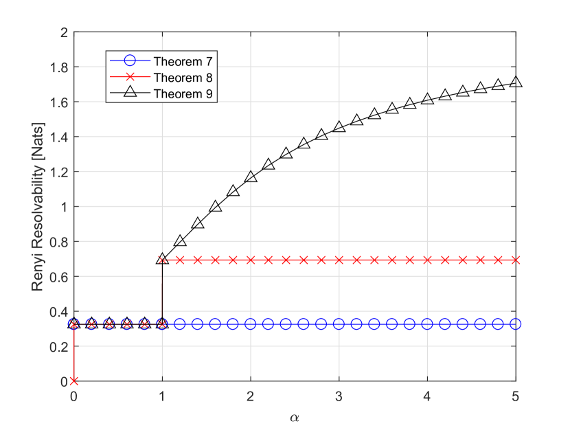
Figure 3: Illustration of the Rényi resolvabilities in Theorems 7, 8, and 9 for $Q_{Y}=\mathsf{Bern}\left(0.1\right)$.

IV Special Case 2: Rényi Intrinsic Randomness

If we set $Q_{Y}$ to the Bernoulli distribution $\mathsf{Bern}(\frac{1}{2})$, then the distribution approximation problem reduces to the intrinsic randomness problem, which can be seen as a “dual” problem of the source resolvability problem. Consider simulating a uniform random variable $M_{n}$ that is uniformly distributed over $\mathcal{M}_{n}:=[1:\mathsf{M}]$ with $\mathsf{M}:=\lceil e^{n\widehat{R}}\rceil$ using a memoryless source $X^{n}\sim P_{X}^{n}$. The rate $\widehat{R}$ here is approximately equal to $\log 2$ times the rate $R$ in Section II with $Q_{Y}$ set to $\mathsf{Bern}(\frac{1}{2})$. Given the distribution $P_{X}$, we wish to maximize the rate $\widehat{R}$ such that the distribution of $M_{n}:=f(X^{n})$ forms a good approximation to the target distribution $Q_{M_{n}}:=\mathrm{Unif}[1:\mathsf{M}]$.

IV-A Asymptotics of Rényi Divergences

We consider the Rényi divergences $D_{\alpha}(P_{M_{n}}\|Q_{M_{n}}),D_{\alpha}(Q_{M_{n}}\|P_{M_{n}})$, and $D_{\alpha}^{\mathsf{max}}(P_{M_{n}},Q_{M_{n}})$. The asymptotics of these measures are respectively characterized in the following corollaries. These results respectively follow from Theorems 1, 2, and 3 by setting $Q_{Y}=\mathsf{Bern}(\frac{1}{2})$.

Corollary 4 (Asymptotics of $\frac{1}{n}D_{\alpha}(P_{M_{n}}\|Q_{M_{n}})$).

For any $\alpha\in[0,\infty]$, we have

$$\lim_{n\to\infty}\frac{1}{n}\inf_{f}D_{\alpha}(P_{M_{n}}\|Q_{M_{n}})$$

$$=\begin{cases}\left[\widehat{R}-H_{\alpha}(P_{X})\right]^{+}&\alpha\in\{0\}\cup[1,\infty]\\ \max_{t\in[0,1]}\left\{t\widehat{R}-tH_{\frac{1}{1-\frac{\alpha-1}{\alpha}t}}(P_{X})\right\}&\alpha\in(0,1)\end{cases}.$$ (55)

Remark 15.

The case $\alpha\in[0,2]$ was shown by Hayashi and Tan [22]. Hence our results for $\alpha\in(2,\infty]$ are new.

Corollary 5 (Asymptotics of $\frac{1}{n}D_{\alpha}(Q_{M_{n}}\|P_{M_{n}})$).

For any $\alpha\in[0,\infty]$, we have

$$\lim_{n\to\infty}\frac{1}{n}\inf_{f}D_{\alpha}(Q_{M_{n}}\|P_{M_{n}})$$

$$=\begin{cases}\sup_{t\in[0,\infty)}\left\{t\widehat{R}-tH_{\frac{1}{1+t}}(P_{X})\right\},&\alpha\in[1,\infty]\\ \frac{\alpha}{1-\alpha}\max_{t\in[0,1]}\left\{t\widehat{R}-tH_{\frac{1}{1+\frac{\alpha}{1-\alpha}t}}(P_{X})\right\},&\alpha\in(0,1)\\ 0,&\alpha=0\end{cases}$$ (56)

Remark 16.

If $\widehat{R}>H_{0}(P_{X})$, then $\lim_{n\to\infty}\frac{1}{n}\inf_{f}D_{\alpha}(Q_{M_{n}}\|P_{M_{n}})=\infty,\alpha\in[1,\infty]$.

Corollary 6 (Asymptotics of $\frac{1}{n}D_{\alpha}^{\mathsf{max}}(P_{Y^{n}},Q_{Y}^{n})$).

For any $\alpha\in[0,\infty]$, we have

$$\lim_{n\to\infty}\frac{1}{n}\inf_{f}D_{\alpha}^{\mathsf{max}}(P_{Y^{n}},Q_{Y}^{n})$$

$$=\begin{cases}\max\biggl{\{}\left[\widehat{R}-H_{\alpha}(P_{X})\right]^{+},\\ \quad\sup_{t\in[0,\infty)}\left\{t\widehat{R}-tH_{\frac{1}{1+t}}(P_{X})\right\}\biggr{\}},&\alpha\in[1,\infty]\\ \max_{t\in[0,1]}\max_{t^{\prime}\in[0,1]}\\ \quad\left\{tb(t^{\prime})\widehat{R}-tb(t^{\prime})H_{\frac{a(t^{\prime})}{a(t^{\prime})+tb(t^{\prime})}}(P_{X})\right\},&\alpha\in(0,1)\\ \left[\widehat{R}-H_{0}(P_{X})\right]^{+},&\alpha=0\end{cases}$$ (57)

where $a(t^{\prime})$ and $b(t^{\prime})$ are defined in (28) and (29).

IV-B Rényi Intrinsic Randomness

As shown in the theorems above, when the rate is large, the normalized Rényi divergences $\frac{1}{n}D_{\alpha}(P_{M_{n}}\|Q_{M_{n}}),\frac{1}{n}D_{\alpha}(Q_{M_{n}}\|P_{M_{n}})$, and $\frac{1}{n}D_{\alpha}^{\mathsf{max}}(P_{M_{n}},Q_{M_{n}})$ converge to a positive number; however when the rate is small enough, the normalized Rényi divergences converge to zero. The threshold rate, named Rényi intrinsic randomness, represents the maximum possible rate to satisfy that the distribution induced by a code well approximates the target uniform distribution. We characterize the Rényi intrinsic randomness in the following theorems. The Rényi intrinsic randomness for normalized divergences of all orders and the Rényi intrinsic randomness for unnormalized divergences of orders in $[0,1]\cup\left\{\infty\right\}$ are direct consequences of Theorems 4, 5, and 6. Hence we only need focus on the cases for unnormalized divergences of orders in $(1,\infty)$. Furthermore, the converse parts for these cases follow from the fact the unnormalized divergences are stronger than the normalized versions. Hence we only prove the achievability parts. The proofs are provided in Appendices K, L, and M, respectively.

Theorem 10 (Rényi Intrinsic Randomness).

For any $\alpha\in[0,\infty]$, we have

$$\sup\left\{\widehat{R}:\frac{1}{n}D_{\alpha}(P_{M_{n}}\|Q_{M_{n}})\rightarrow 0\right\}$$

$$=\sup\left\{\widehat{R}:D_{\alpha}(P_{M_{n}}\|Q_{M_{n}})\rightarrow 0\right\}$$

$$=\begin{cases}H_{\alpha}(P_{X})&\alpha\in\{0\}\cup[1,\infty]\\ H(P_{X})&\alpha\in(0,1)\end{cases}.$$ (58)

Remark 17.

The case $\alpha=1$ and the normalized divergence (i.e., the normalized relative entropy case) was shown in [1]. The case $\alpha=1$ and the unnormalized divergence (i.e., the unnormalized relative entropy case) was shown by Hayashi [23]. The result for the unnormalized Rényi divergence with $\alpha\in(0,1)$ can be obtained by combining two observations: 1) the achievability for $D(P_{Y^{n}}\|Q_{Y}^{n})$ implies the achievability for this case; 2) by Pinsker’s inequality [3], the result under the TV distance measure [1] implies the converse for $\alpha\in(0,1)$. The case $\alpha\in[0,2]$ was shown by Hayashi and Tan [22]. Hence our results for $\alpha\in(2,\infty]$ are new.

Theorem 11 (Rényi Intrinsic Randomness).

For any $\alpha\in[0,\infty]$, we have

$$\sup\left\{\widehat{R}:\frac{1}{n}D_{\alpha}(Q_{M_{n}}\|P_{M_{n}})\rightarrow 0\right\}$$

$$=\sup\left\{\widehat{R}:D_{\alpha}(Q_{M_{n}}\|P_{M_{n}})\rightarrow 0\right\}$$

$$=\begin{cases}H(P_{X}),&\alpha\in(0,\infty]\\ \infty,&\alpha=0\end{cases}$$ (59)

Remark 18.

The case $\alpha=1$ was shown by Hayashi [23]. Our results for all orders $\alpha\in[0,1)\cup(1,\infty]$ are new.

Theorem 12 (Rényi Intrinsic Randomness).

For any $\alpha\in[0,\infty]$, we have

$$\sup\left\{\widehat{R}:\frac{1}{n}D_{\alpha}^{\mathsf{max}}(P_{M_{n}},Q_{M_{n}})\rightarrow 0\right\}$$

$$=\sup\left\{\widehat{R}:D_{\alpha}^{\mathsf{max}}(P_{M_{n}},Q_{M_{n}})\rightarrow 0\right\}$$

$$=\begin{cases}H_{\alpha}(P_{X}),&\alpha\in\{0\}\cup[1,\infty]\\ H(P_{X}),&\alpha\in(0,1)\end{cases}$$ (60)

Theorems 10, 11, and 12 are illustrated in Fig. 4.

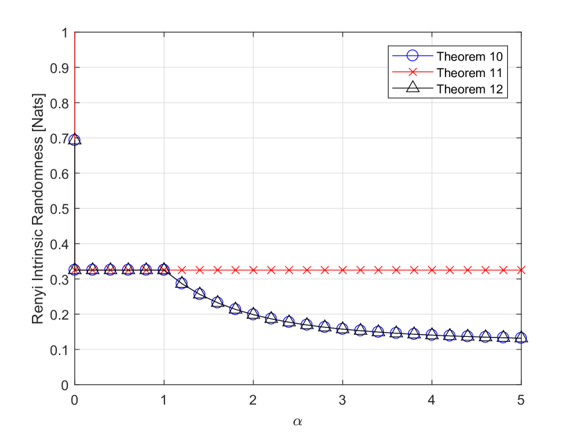
Figure 4: Illustration of the Rényi intrinsic randomness in Theorems 10, 11, and 12 for $P_{X}=\mathsf{Bern}\left(0.1\right)$.

V Concluding Remarks

In this paper, we studied generalized versions of random variable simulation problem or distribution approximation problem, in which the (normalized or unnormalized) standard Rényi divergence and max- or sum-Rényi divergence of orders in $[0,\infty]$ are used to measure the level of approximation. As special cases, the source resolvability problem and the intrinsic randomness problem were studied as well.

Our results on the distribution approximation problem extend those by Han [1] and by Kumagai and Hayashi [2], as we consider Rényi divergences with all orders in $[0,\infty]$ instead of the TV distance or the special case with order $\frac{1}{2}$. Similarly, our source resolvability results extend those by Han and Verdú [4], by Hayashi [5, 6], and by Yu and Tan [8] for the source resolvability case, and our intrinsic randomness results extend those by Vembu and Verdú [9], by Han [1], and by Hayashi and Tan [22].

V-A Open Problem

In Theorems 4, 5, and 6, we completely characterized the Rényi conversion rates only for $\alpha\in[0,1]\cup\left\{\infty\right\}$. But the cases for $\alpha\in(1,\infty)$ are still open. We believe that analogous to the case $\alpha\in[0,1]\cup\left\{\infty\right\}$, the unnormalized version of Rényi conversion rate for $\alpha\in(1,\infty)$ is also equal to the corresponding normalized version with the same $\alpha$.

V-B Applications

Similar to other results concerning simulation of random variables, our results can be applied to the analysis of Monte Carlo methods, randomized algorithms (or random coding), and cryptography. In the following we apply our results to information-theoretic security. To illustrate this point, we consider the Shannon cipher system with a guessing wiretapper that was studied in [24]. In the Shannon cipher system, the sender and the legitimate receiver share a secret key $K_{n}\sim\mathrm{Unif}\left[1:e^{nR}\right]$, and they want to communicate a source $X^{n}\sim P_{X}^{n}$ with zero-error (using a variable-length code $M_{n}=f(X^{n},K_{n})$ and $X^{n}=f^{-1}(M_{n},K_{n})$) from the sender to the legitimate receiver through a public noiseless channel with sufficiently large capacity. However, the cryptogram $M_{n}$ is overheard by a wiretapper, who has a test mechanism by which s/he can identify whether any given candidate message $\widehat{X}^{n}$ is the true message. Upon the code $f$ used by the sender and legitimate receiver and the received cryptogram $M_{n}$, the wiretapper conducts an optimal sequential guessing strategy, i.e., an ordered list of guesses $\mathcal{L}\left(m\right):=\left\{\widehat{x}_{1}^{n}\left(m\right),\widehat{x}_{2}^{n}\left(m\right),..\right\}$ with $\widehat{x}_{i}^{n}\left(m\right)$ corresponding to the $i$-th largest probability value of $P_{X^{n}|M_{n}}(\cdot|m)$ for any given $M_{n}=m$. It is obvious that such a guessing scheme based on maximizing the posterior probability minimizes the expectation or positive-order moments of the number of guesses. Let the random variable $G(X^{n}|M_{n})$ denote the number of guesses of the wiretapper until identification of the true message. Then for $\rho>0$, the $\rho$-th moment of $G(X^{n}|M_{n})$ can be also expressed as

$$\mathbb{E}\left[G(X^{n}|M_{n})^{\rho}\right]=\inf_{\left\{\mathcal{L}(m)\right\}}\left[\sum_{i=1}^{\infty}i^{\rho}\cdot\mathbb{P}\left\{\left.\mathcal{L}(M_{n})\right|_{i}=X^{n}\right\}\right],$$ (61)

where $\left.\mathcal{L}(M_{n})\right|_{i}$ denotes the $i$-th element of $\mathcal{L}(M_{n})$. For $\rho>0$, the guessing exponents are defined as

$$E^{+}(R,\rho) :=\limsup_{n\to\infty}\sup_{f}\frac{1}{n}\log\mathbb{E}\left[G(X^{n}|M_{n})^{\rho}\right]$$ (62)

$$E^{-}(R,\rho) :=\liminf_{n\to\infty}\sup_{f}\frac{1}{n}\log\mathbb{E}\left[G(X^{n}|M_{n})^{\rho}\right].$$ (63)

Merhav and Arikan [24] showed that

$$E^{+}(R,\rho)=E^{-}(R,\rho)=E(R,\rho)$$ (64)

$$:=\max_{Q_{X}}\left\{\rho\min\left\{H(Q_{X}),R\right\}-D(Q_{X}\|P_{X})\right\}.$$ (65)

Now we consider a variant of this problem. Suppose the secret key $K_{n}$ is replaced by a memoryless source $Y^{n}\sim P_{Y}^{n}$. Correspondingly, denote the guessing exponents for this case as $\widetilde{E}^{+}(P_{Y},\rho)$ and $\widetilde{E}^{-}(P_{Y},\rho)$. Next, we apply our results to this new problem.

For the achievability part, we use $Y^{n}$ to simulate a key $K_{n}\sim Q_{K_{n}}:=\mathrm{Unif}\left[1:e^{nR}\right]$ by our simulation code $K_{n}=g(Y^{n})$. Assume $P_{K_{n}}$ is the key distribution induced by a generator $K_{n}=g(Y^{n})$. Then Corollary 4 implies that $\inf_{g}\frac{1}{n}D_{\infty}(Q_{K_{n}}\|P_{K_{n}})\leq\sup_{t\in[0,\infty)}\left\{tR-tH_{\frac{1}{1+t}}(P_{Y})\right\}$. Furthermore, for any $f$ and any $\left\{\mathcal{L}(m)\right\}$,

$$\frac{1}{n}\log\frac{\mathbb{E}_{P_{K_{n}}P_{X}^{n}}\left[\sum_{i=1}^{\infty}i^{\rho}\cdot 1\left\{\left.\mathcal{L}(f(X^{n},K_{n}))\right|_{i}=X^{n}\right\}\right]}{\mathbb{E}_{Q_{K_{n}}P_{X}^{n}}\left[\sum_{i=1}^{\infty}i^{\rho}\cdot 1\left\{\left.\mathcal{L}(f(X^{n},K_{n}))\right|_{i}=X^{n}\right\}\right]}$$

$$\geq-\frac{1}{n}D_{\infty}(Q_{K_{n}}\|P_{K_{n}}).$$ (66)

On the other hand, (64) implies

$$\lim_{n\to\infty}\sup_{f}\frac{1}{n}\log\inf_{\left\{\mathcal{L}(m)\right\}}\mathbb{E}_{Q_{K_{n}}P_{X}^{n}}$$

$$\quad\left[\sum_{i=1}^{\infty}i^{\rho}\cdot 1\left\{\left.\mathcal{L}(f(X^{n},K_{n}))\right|_{i}=X^{n}\right\}\right]=E(R,\rho).$$ (67)

Hence the guessing exponent functions are bounded as follows.

$$\sup_{R\geq 0}\left\{E(R,\rho)-\sup_{t\in[0,\infty)}\left\{tR-tH_{\frac{1}{1+t}}(P_{Y})\right\}\right\}$$

$$\leq\widetilde{E}^{-}(P_{Y},\rho)\leq\widetilde{E}^{+}(P_{Y},\rho).$$ (68)

For the converse part, we use a key $K_{n}\sim Q_{K_{n}}:=\mathrm{Unif}\left[1:e^{nR}\right]$ to simulate a memoryless source $Y^{n}\sim P_{Y}^{n}$ by our simulation code $Y^{n}=g(K_{n})$. Similarly, by our Corollary 1, we obtain the following converse result.

$$\widetilde{E}^{-}(P_{Y},\rho)\leq\widetilde{E}^{+}(P_{Y},\rho)\leq E(H_{0}(P_{Y}),\rho).$$ (69)

When $P_{X}$ is uniform, the bounds in (68) and (69) coincide, and they reduce to the result in (64). However, in general, the bounds in (68) and (69) do not coincide. Furthermore, it is worth noting that the analysis here also applies to variants of any information-theoretic security problem in which a key (uniform random variable) is replaced with a memoryless source, as long as the objective of the problem is to minimize or maximize the some expectation.

The results derived in this paper can be also applied to the information-theoretic security problems with the information leakage measured by Rényi divergences. Recently, in [25], Theorem 7 has been used to establish the equivalence between the exact and $\infty$-Rényi common informations by the present authors. Here the $\infty$-Rényi common information is defined in a distributed source simulation problem with the approximation between the generated distribution and the target distribution measured by the Rényi divergence of order $\infty$. In [25], Rényi divergences were used to build a bridge between Wyner’s common information and the exact common information. Therefore, in consideration of the importance of Rényi divergences in connecting different simulation problems, it is significant to consider Rényi divergences as performance indicators for simulation problems, and also for information-theoretic security problems.

Appendix A Preliminaries for the Proofs

For a function $f:\mathcal{X}\to\mathcal{Y}$, and any subsets $\mathcal{A}\subseteq\mathcal{X}$ and $\mathcal{B}\subseteq\mathcal{Y}$, define $f\left(\mathcal{A}\right):=\left\{f(x):x\in\mathcal{A}\right\}$, and $f^{-1}(\mathcal{B}):=\left\{x\in\mathcal{X}:f(x)\in\mathcal{B}\right\}$. We write $f(n)\mathrel{\dot{\leq}}g(n)$ if $\limsup_{n\to\infty}\frac{1}{n}\log\frac{f(n)}{g(n)}\leq 0$. In addition, $f(n)\doteq g(n)$ means $f(n)\mathrel{\dot{\leq}}g(n)$ and $g(n)\mathrel{\dot{\leq}}f(n)$. We use $o(1)$ to denote generic sequences tending to zero as $n\rightarrow\infty$. For $a\in\mathbb{R}$, $[a]^{+}:=\max\{a,0\}$ denotes positive clipping. For simplicity, in the proof part, we denote $s=\alpha-1$.

A-A Lemmas

The following fundamental lemmas will be used in our proofs.

Lemma 2.

[8]

1. Assume $\mathcal{X}$ is a finite set. Then for any $P_{X}\in\mathcal{P}\left(\mathcal{X}\right)$, one can find a sequence of types $P_{X}^{\left(n\right)}\in\mathcal{P}^{\left(n\right)}\left(\mathcal{X}\right),n\in\mathbb{N}$ such that $\big{|}P_{X}-P_{X}^{\left(n\right)}\big{|}\leq\frac{\left|\mathcal{X}\right|}{2n}$ as $n\rightarrow\infty$.

2. Assume $\mathcal{X},\mathcal{Y}$ are finite sets. Then for any sequence of types $P_{X}^{\left(n\right)}\in\mathcal{P}^{\left(n\right)}\left(\mathcal{X}\right),n\in\mathbb{N}$ and any $P_{Y|X}\in\mathcal{P}\left(\mathcal{Y}|\mathcal{X}\right)$, one can find a sequence of conditional types $V_{Y|X}^{(n)}\in\mathcal{P}^{\left(n\right)}\big{(}\mathcal{Y}|P_{X}^{\left(n\right)}\big{)},n\in\mathbb{N}$ such that $\big{|}P_{X}^{\left(n\right)}P_{Y|X}-P_{X}^{\left(n\right)}V_{Y|X}^{(n)}\big{|}\leq\frac{\left|\mathcal{X}\right|\left|\mathcal{Y}\right|}{2n}$ as $n\rightarrow\infty$.

We also need the following property concerning the optimization over the set of types and conditional types.

Lemma 3.

[8]

1. Assume $\mathcal{X}$ is a finite set. Then for any continuous (under TV distance) function $f:\mathcal{P}\left(\mathcal{X}\right)\to\mathbb{R}$, we have

   $$\lim_{n\rightarrow\infty}\min_{P_{X}\in\mathcal{P}^{\left(n\right)}\left(\mathcal{X}\right)}f\left(P_{X}\right)=\min_{P_{X}\in\mathcal{P}\left(\mathcal{X}\right)}f\left(P_{X}\right).$$ (70)

2. Assume $\mathcal{X},\mathcal{Y}$ are finite sets. Then for any continuous function $f:\mathcal{P}\left(\mathcal{X}\times\mathcal{Y}\right)\to\mathbb{R}$ and any sequence of types $P_{X}^{\left(n\right)}\in\mathcal{P}^{\left(n\right)}\left(\mathcal{X}\right),n\in\mathbb{N}$, we have

   $$\min_{P_{Y|X}\in\mathcal{P}^{\left(n\right)}(\mathcal{Y}|P_{X}^{\left(n\right)})}f\big{(}P_{X}^{\left(n\right)}P_{Y|X}\big{)}$$

   $$=\min_{P_{Y|X}\in\mathcal{P}\left(\mathcal{Y}|\mathcal{X}\right)}f\big{(}P_{X}^{\left(n\right)}P_{Y|X}\big{)}+o\left(1\right).$$ (71)

Remark 19.

We have

$$\lim_{n\rightarrow\infty}\min_{P_{Y|X}\in\mathcal{P}^{\left(n\right)}(\mathcal{Y}|P_{X}^{\left(n\right)})}f\big{(}P_{X}^{\left(n\right)}P_{Y|X}\big{)}$$

$$=\lim_{n\rightarrow\infty}\min_{P_{Y|X}\in\mathcal{P}\left(\mathcal{Y}|\mathcal{X}\right)}f\big{(}P_{X}^{\left(n\right)}P_{Y|X}\big{)}$$ (72)

if either one of the limits above exists.

We also need the following lemmas. Lemmas 4, 6, 7, and 8 follow from basic inequalities and basic properties (continuity, monotonicity, and convexity) of functions. To save space, the proofs are omitted.

Lemma 4.

Assume $f(z)$ and $g(z)$ are continuous functions defined on a compact set $\mathcal{Z}\subseteq\mathbb{R}^{n}$ for some positive integer $n$. Define $h(t):=\min_{z\in\mathcal{Z}:g(z)\leq t}f(z)$. Then $h(t)$ is a also continuous function.

Lemma 5.

[26, Problem 4.15(f)] Assume $\left\{a_{i}\right\}$ are non-negative real numbers. Then for $p\geq 1$, we have

$$\sum_{i}a_{i}^{p}\leq\left(\sum_{i}a_{i}\right)^{p},$$ (73)

and for $0<p\leq 1$, we have

$$\sum_{i}a_{i}^{p}\geq\left(\sum_{i}a_{i}\right)^{p}.$$ (74)

Lemma 6.

$$\left(1+x\right)^{s}\leq 1+x^{s}, \qquad x\geq 0,\;0\leq s\leq 1,$$ (75)

$$\left(1+x\right)^{s}\leq 1+sx+x^{s}, \qquad x\geq 0,\;1\leq s\leq 2,$$ (76)

$$\left(1+x\right)^{s}\leq 1+s\left(2^{s-1}-1\right)x+x^{s}, \qquad 0\leq x\leq 1,\;s\geq 2.$$ (77)

Lemma 7.

Assume $\sum_{i=1}^{n}b_{i}=m$. Then we have that for $\beta\leq 0$ or $\beta\geq 1$, $\frac{1}{n}\sum_{i=1}^{n}b_{i}^{\beta}\geq\left(\frac{m}{n}\right)^{\beta}$; for $0<\beta<1$, $\frac{1}{n}\sum_{i=1}^{n}b_{i}^{\beta}\leq\left(\frac{m}{n}\right)^{\beta}$. Moreover, if $m<n$ and $b_{i}\in\{0\}\cup\mathbb{N}$, we have that for $\beta\leq 0$ or $\beta\geq 1$, $\frac{1}{n}\sum_{i=1}^{n}b_{i}^{\beta}\geq\frac{m}{n}$; for $0<\beta<1$, $\frac{1}{n}\sum_{i=1}^{n}b_{i}^{\beta}\leq\frac{m}{n}$.

Lemma 8.

For any $a\geq 0$ and any $b$,

$$\sup_{\widetilde{P}_{X}\in\mathcal{P}\left(\mathcal{X}\right)}\left\{aH(\widetilde{P}_{X})+b\sum_{x}\widetilde{P}_{X}(x)\log P_{X}(x)\right\}$$

$$=\left(a-b\right)H_{\frac{b}{a}}(P_{X}).$$ (78)

For any $a\leq 0$ and any $b$,

$$\inf_{\widetilde{P}_{X}\in\mathcal{P}\left(\mathcal{X}\right)}\left\{aH(\widetilde{P}_{X})+b\sum_{x}\widetilde{P}_{X}(x)\log P_{X}(x)\right\}$$

$$=\left(a-b\right)H_{\frac{b}{a}}(P_{X}).$$ (79)

A-B Information Spectrum Exponents

Since information spectrum exponents are important in our proofs of the results in this paper, they will be introduced in the following. Furthermore, as fundamental information-theoretic quantities, investigating information spectrum exponents are of independent interest.

For a general distribution $P_{X^{n}}$, define $F_{P_{X^{n}}}(\jmath):=P_{X^{n}}\left(x^{n}:-\frac{1}{n}\log P_{X^{n}}(x^{n})<\jmath\right)$ and $F_{P_{X^{n}}}^{-1}(\theta):=\sup\left\{\jmath:F_{P_{X^{n}}}(\jmath)\leq\theta\right\}$. Now consider a product distribution $P_{X}^{n}$ with $P_{X}$ defined on a finite set $\mathcal{X}$. Define the information spectrum exponents (or entropy spectrum exponents) for distribution $P_{X}$ as

$$E_{P_{X}}(\jmath) :=\lim_{n\to\infty}-\frac{1}{n}\log F_{P_{X}^{n}}(\jmath)$$ (80)

$$\widehat{E}_{P_{X}}(\jmath) :=\lim_{n\to\infty}-\frac{1}{n}\log\left(1-F_{P_{X}^{n}}(\jmath)\right).$$ (81)

Or simply, define the information spectrum exponent for distribution $P_{X}$ as

$$\widetilde{E}_{P_{X}}(\jmath) :=\max\left\{E_{P_{X}}(\jmath),\widehat{E}_{P_{X}}(\jmath)\right\}.$$ (82)

Since for each $\jmath\geq 0$, either $E_{P_{X}}(\jmath)$ or $\widehat{E}_{P_{X}}(\jmath)$ can be positive (the other one must be zero), the exponent $\widetilde{E}_{P_{X}}(\jmath)$ contains all the information about the exponent pair $\left(E_{P_{X}}(\jmath),\widehat{E}_{P_{X}}(\jmath)\right)$. Moreover, the inverse functions of $E_{P_{X}}(\jmath)$ and $\widehat{E}_{P_{X}}(\jmath)$ are denoted as $E_{P_{X}}^{-1}(\omega)$ and $\widehat{E}_{P_{X}}^{-1}(\omega)$. Then we have the following lemmas. Observe that if $P_{X}$ is uniform, then $\widetilde{E}_{P_{X}}(\jmath)=+\infty$ for all $\jmath$. Hence, in the following, we exclude this trivial case.

Lemma 9 (Information Spectrum Exponents).

Assume $P_{X}$ is not uniform. For $\jmath>H_{\infty}(P_{X})$,

$$E_{P_{X}}(\jmath) =\min_{\widetilde{P}_{X}:-\sum_{x}\widetilde{P}_{X}(x)\log P_{X}(x)\leq\jmath}D(\widetilde{P}_{X}\|P_{X})$$ (83)

$$=\max_{t\in[0,\infty]}\left\{tH_{1+t}(P_{X})-t\jmath\right\},$$ (84)

and for $0\leq\jmath\leq H_{-\infty}(P_{X})$,

$$\widehat{E}_{P_{X}}(\jmath) =\min_{\widetilde{P}_{X}:-\sum_{x}\widetilde{P}_{X}(x)\log P_{X}(x)\geq\jmath}D(\widetilde{P}_{X}\|P_{X})$$ (85)

$$=\max_{t\in[0,\infty]}\left\{-tH_{1-t}(P_{X})+t\jmath\right\}.$$ (86)

For $0\leq\omega<H_{\infty}(P_{X})$,

$$E_{P_{X}}^{-1}(\omega) =\min_{\widetilde{P}_{X}:D(\widetilde{P}_{X}\|P_{X})\leq\omega}-\sum_{x}\widetilde{P}_{X}(x)\log P_{X}(x)$$ (87)

$$=\max_{t\in[0,\infty]}\left\{H_{1+t}(P_{X})-\frac{\omega}{t}\right\},$$ (88)

and for $0\leq\omega\leq H_{-\infty}(P_{X})$,

$$\widehat{E}_{P_{X}}^{-1}(\omega) =\max_{\widetilde{P}_{X}:D(\widetilde{P}_{X}\|P_{X})\leq\omega}-\sum_{x}\widetilde{P}_{X}(x)\log P_{X}(x)$$ (89)

$$=\min_{t\in[0,\infty]}\left\{H_{1-t}(P_{X})+\frac{\omega}{t}\right\}.$$ (90)

Moreover, $E_{P_{X}}(\jmath)$, $\widehat{E}_{P_{X}}(\jmath)$, $E_{P_{X}}^{-1}(\omega)$, and $\widehat{E}_{P_{X}}^{-1}(\omega)$ are continuous on the intervals mentioned above.

Remark 20.

We can use $E_{P_{X}}(\jmath)$, $\widehat{E}_{P_{X}}(\jmath)$, $E_{P_{X}}^{-1}(\omega)$, and $\widehat{E}_{P_{X}}^{-1}(\omega)$ to rewrite $F_{P_{X^{n}}}(\jmath)$, $1-F_{P_{X^{n}}}(\jmath)$, $F_{P_{X}^{n}}^{-1}(\theta)$, and $F_{P_{X}^{n}}^{-1}(1-\theta)$ as follows:

$$F_{P_{X^{n}}}(\jmath) =e^{-n\left(E_{P_{X}}(\jmath)+o(1)\right)}$$ (91)

$$1-F_{P_{X^{n}}}(\jmath) =e^{-n\left(\widehat{E}_{P_{X}}(\jmath)+o(1)\right)}$$ (92)

$$F_{P_{X}^{n}}^{-1}(\theta) =E_{P_{X}}^{-1}(-\frac{1}{n}\log\theta-o(1))$$ (93)

$$F_{P_{X}^{n}}^{-1}(1-\theta) =\widehat{E}_{P_{X}}^{-1}(-\frac{1}{n}\log\theta-o(1)),$$ (94)

where the first two equalities follow from the definitions of $E_{P_{X}}(\jmath)$ and $\widehat{E}_{P_{X}}(\jmath)$, and the last two follow since

$$F_{P_{X}^{n}}^{-1}(\theta) =\sup\left\{\jmath:F_{P_{X}^{n}}(\jmath)\leq\theta\right\}$$ (95)

$$=\sup\left\{\jmath:e^{-n\left(E_{P_{X}}(\jmath)+o(1)\right)}\leq\theta\right\}$$ (96)

$$=\sup\left\{\jmath:E_{P_{X}}(\jmath)\geq-\frac{1}{n}\log\theta-o(1)\right\}$$ (97)

$$=E_{P_{X}}^{-1}(-\frac{1}{n}\log\theta-o(1))$$ (98)

and similarly for $F_{P_{X}^{n}}^{-1}(1-\theta)$.

Lemma 9 follows by large deviation theory [27], and it holds not only for finite alphabets, but also for countably infinite or continuous alphabets (with the probability mass function $P_{X}$ replaced by the corresponding probability density function or the Radon-Nikodym derivative and the summation replaced by the corresponding integration). Note that $tH_{1-t}(P_{X})=\log\mathbb{E}\left[e^{-t\log P_{X}(x)}\right]$ is the logarithmic moment generating function respect to the self-information (or self-entropy) $-\log P_{X}(x)$, and (84) and (86) are the Fenchel–Legendre transform of $tH_{1-t}(P_{X})$. Furthermore, by [27, Lemma 2.2.31], $tH_{1-t}(P_{X})$ is convex in $t\in\mathbb{R}$.

Note that in (83) and (85), the minima are attained by the $\alpha$-tilted distributions $P_{X}^{(\alpha)}(\cdot)=\frac{P_{X}^{\alpha}(\cdot)}{\sum_{x^{\prime}}P_{X}^{\alpha}(x^{\prime})}$ with $\alpha$ satisfying $\jmath=H_{\alpha}^{\mathrm{u}}(P_{X})$. Hence $P_{X}^{(\alpha)}$ can be seen as a dominant “asymptotic type”. We have the following lemma.

Lemma 10.

$\widetilde{E}_{P_{X}}(\jmath)$ can be expressed as the following parametric representation with $\alpha\in[-\infty,\infty]$.

$$\begin{cases}\jmath=H_{\alpha}^{\mathrm{u}}(P_{X}),\\ \widetilde{E}_{P_{X}}=D\left(P_{X}^{(\alpha)}\|P_{X}\right).\end{cases}$$

Specialized to the case $\alpha=0$, it reduces to that

$$\widetilde{E}_{P_{X}}(H^{\mathrm{u}}(P_{X}))=\widehat{E}_{P_{X}}(H^{\mathrm{u}}(P_{X})) =D(\mathrm{Unif}\left(\mathcal{X}\right)\|P_{X}).$$ (99)

The information spectrum limit

$$\lim_{n\to\infty}F_{P_{X}^{n}}(\jmath)=\begin{cases}0&\jmath<H(P_{X})\\ \frac{1}{2}&\jmath=H(P_{X})\\ 1&\jmath>H(P_{X})\end{cases}$$ (100)

and the information spectrum exponent $\widetilde{E}_{P_{X}}(\jmath)$ are illustrated in Fig. 5.

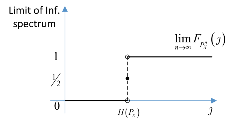
(a) The information spectrum limit

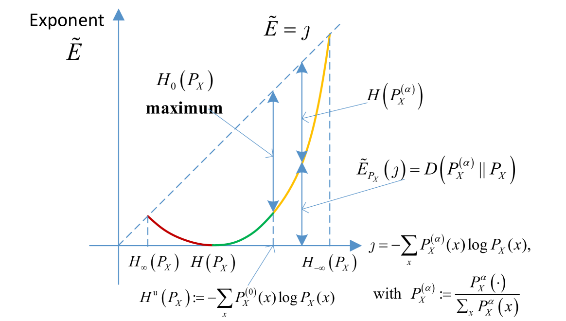
(b) The information spectrum exponent

Figure 5: Illustrations of the information spectrum limit and exponent. Note that in the bottom subfigure, the left (resp. right) endpoint of the information spectrum exponent $\widetilde{E}_{P_{X}}(\jmath)$ should be strictly lower than the line $\widetilde{E}=\jmath$ if there are multiple maximum (resp. minimum) probability values in $P_{X}$.

Lemma 11 (Comparison of Exponents).

Assume both $P_{X}$ and $Q_{Y}$ are not uniform. Then we have

$$\frac{1}{R}E_{P_{X}}(R\jmath)>E_{Q_{Y}}(\jmath),\>\forall\jmath\in\frac{1}{R}[H_{\infty}(P_{X}),H(P_{X})]$$

$$\Longleftrightarrow\qquad R<\min_{t\in[1,\infty]}\frac{H_{t}(P_{X})}{H_{t}(Q_{Y})};$$ (101)

$$\frac{1}{R}\widehat{E}_{P_{X}}(R\jmath)<\widehat{E}_{Q_{Y}}(\jmath),\>\forall\jmath\in\frac{1}{R}[H(P_{X}),H_{-\infty}(P_{X})]$$

$$\Longleftrightarrow\qquad R<\min_{t\in[-\infty,1]}\frac{H_{t}(P_{X})}{H_{t}(Q_{Y})}.$$ (102)

Furthermore, the equivalence in (102) can be divided into the following two parts:

$$\begin{cases}\frac{1}{R}\widehat{E}_{P_{X}}(R\jmath)<\widehat{E}_{Q_{Y}}(\jmath),\>\forall\jmath\in\frac{1}{R}[H(P_{X}),H^{\mathrm{u}}(P_{X})]\\ R<\frac{H_{0}(P_{X})}{H_{0}(Q_{Y})}\end{cases}$$

$$\Longleftrightarrow\qquad R<\min_{t\in[0,1]}\frac{H_{t}(P_{X})}{H_{t}(Q_{Y})};$$ (103)

$$\begin{cases}\frac{1}{R}\widehat{E}_{P_{X}}(R\jmath)<\widehat{E}_{Q_{Y}}(\jmath),\>\forall\jmath\in\frac{1}{R}[H^{\mathrm{u}}(P_{X}),H_{-\infty}(P_{X})]\\ R<\frac{H_{0}(P_{X})}{H_{0}(Q_{Y})}\end{cases}$$

$$\Longleftrightarrow\qquad R<\min_{t\in[-\infty,0]}\frac{H_{t}(P_{X})}{H_{t}(Q_{Y})}.$$ (104)

In addition, the equivalences in (101)-(104) also hold if all the “$<$” are replaced with “$\leq$”.

Proof:

Here we only provide a proof for the equivalence in (103). Other equivalences can be proven similarly.

Proof of “$\Longleftarrow$”: Observe that the RHS of (103) implies

$$H_{t}(Q_{Y})<\frac{1}{R}H_{t}(P_{X}),\forall t\in[0,1].$$ (105)

Hence we have

$$\max_{t\in[0,1]}\left\{-\frac{t}{R}H_{1-t}(P_{X})+t\jmath\right\}$$

$$<\max_{t\in[0,1]}\left\{-tH_{1-t}(Q_{Y})+t\jmath\right\},\forall\jmath.$$ (106)

Observe that $-\frac{t}{R}H_{1-t}(P_{X})+t\jmath$ is concave in $t$ (which can be shown by a similar proof to that of [8, Lemma 7], or directly by [27, Lemma 2.2.31] since $tH_{1-t}(P_{X})=\log\mathbb{E}\left[e^{-t\log P_{X}(x)}\right]$ is the logarithmic moment generating function respect to the self-information $-\log P_{X}(x)$), and for $\jmath\in\frac{1}{R}[H(P_{X}),H^{\mathrm{u}}(P_{X})]$, the extreme point of $t\mapsto-\frac{t}{R}H_{1-t}(P_{X})+t\jmath$ is in $[0,1]$. We have for $\jmath\in\frac{1}{R}[H(P_{X}),H^{\mathrm{u}}(P_{X})]$,

$$\max_{t\in[0,1]}\left\{-\frac{t}{R}H_{1-t}(P_{X})+t\jmath\right\}$$

$$=\max_{t\in[0,\infty]}\left\{-\frac{t}{R}H_{1-t}(P_{X})+t\jmath\right\}.$$ (107)

Hence for $\jmath\in\frac{1}{R}[H(P_{X}),H^{\mathrm{u}}(P_{X})]$,

$$\max_{t\in[0,\infty]}\left\{-\frac{t}{R}H_{1-t}(P_{X})+t\jmath\right\}$$

$$<\max_{t\in[0,1]}\left\{-tH_{1-t}(Q_{Y})+t\jmath\right\}$$ (108)

$$\leq\max_{t\in[0,\infty]}\left\{-tH_{1-t}(Q_{Y})+t\jmath\right\},$$ (109)

which, by Lemma 9, implies the LHS of (103).

Proof of “$\Longrightarrow$”: The LHS of (103) implies for $\jmath\in\frac{1}{R}[H(P_{X}),H^{\mathrm{u}}(P_{X})]$,

$$\max_{t\in[0,\infty]}\left\{-\frac{t}{R}H_{1-t}(P_{X})+t\jmath\right\}$$

$$<\max_{t\in[0,\infty]}\left\{-tH_{1-t}(Q_{Y})+t\jmath\right\},$$ (110)

By setting $\jmath=\frac{1}{R}H(P_{X})$, we have $\frac{1}{R}H(P_{X})>H(Q_{Y})$.

On the other hand, given $\jmath\in[H(Q_{Y}),H_{-\infty}(Q_{Y})]$, the maximum in the RHS of (110) is attained at $g^{-1}(\jmath)$ which is a value $t$ satisfying $\jmath=g(t):=\frac{\partial}{\partial t}\left(tH_{1-t}(Q_{Y})\right)=-\frac{1}{\sum_{y\in\mathcal{Y}}Q_{Y}^{1-t}(y)}\sum_{y\in\mathcal{Y}}Q_{Y}^{1-t}(y)\log Q_{Y}(y)=H_{1-t}^{\mathrm{u}}(Q_{Y})$. Here $g(t)$ is a increasing function since $tH_{1-t}(Q_{Y})$ is convex. Hence for $\jmath$ running from $H(Q_{Y})$ to $\frac{1}{R}H^{\mathrm{u}}(P_{X})$, $g^{-1}(\jmath)$ runs from $0$ to $t_{0}$, where $t_{0}$ is the solution to $\frac{1}{R}H^{\mathrm{u}}(P_{X})=g(t_{0})$. Observe $g^{-1}(\jmath)$ is continuous. Hence for each $t^{\prime}\in[0,t_{0}]$, we can find a $\jmath^{\prime}\in[H(Q_{Y}),\frac{1}{R}H^{\mathrm{u}}(P_{X})]$ such that $g^{-1}(\jmath^{\prime})=t^{\prime}$. For such $\left(\jmath^{\prime},t^{\prime}\right)$, we have

$$-t^{\prime}H_{1-t^{\prime}}(Q_{Y})+t^{\prime}\jmath^{\prime}$$

$$=\max_{t\in[0,\infty]}\left\{-tH_{1-t}(Q_{Y})+t\jmath^{\prime}\right\}$$ (111)

$$>\max_{t\in[0,\infty]}\left\{-\frac{t}{R}H_{1-t}(P_{X})+t\jmath^{\prime}\right\}$$ (112)

$$\geq-\frac{t^{\prime}}{R}H_{1-t^{\prime}}(P_{X})+t^{\prime}\jmath^{\prime}.$$ (113)

That is, for $t^{\prime}\in[0,t_{0}]$,

$$RH_{1-t^{\prime}}(Q_{Y})<H_{1-t^{\prime}}(P_{X}).$$ (114)

If $t_{0}<1$, then $\frac{1}{R}H^{\mathrm{u}}(P_{X})<H^{\mathrm{u}}(Q_{Y})$. The derivative of $\widehat{E}_{Q_{Y}}(\jmath)$ is $g^{-1}(\jmath)$ at $\jmath$, where $g(t)$ is defined above. For $\jmath\in[\frac{1}{R}H^{\mathrm{u}}(P_{X}),H^{\mathrm{u}}(Q_{Y})]$, $g^{-1}(\jmath)\in[t_{0},1]$. Observe that $\widehat{E}_{Q_{Y}}(\jmath)$ and $\frac{1}{R}\widehat{E}_{P_{X}}(R\jmath)$ are convex, and $-H_{0}(Q_{Y})+\jmath$ and $-\frac{1}{R}H_{0}(P_{X})+\jmath$ are respectively the tangent lines of $\widehat{E}_{Q_{Y}}(\jmath)$ at $\jmath_{0}=H^{\mathrm{u}}(Q_{Y})$ and $\frac{1}{R}\widehat{E}_{P_{X}}(R\jmath)$ at $\jmath_{0}=\frac{1}{R}H^{\mathrm{u}}(P_{X})$. Hence combining with the assumption $R<\frac{H_{0}(P_{X})}{H_{0}(Q_{Y})}$, we have $\widehat{E}_{Q_{Y}}(\jmath)\geq-H_{0}(Q_{Y})+\jmath>-\frac{1}{R}H_{0}(P_{X})+\jmath$. Moreover, we also have that tangent lines of $\frac{1}{R}\widehat{E}_{P_{X}}(R\jmath)$ at $\jmath_{0}<\frac{1}{R}H^{\mathrm{u}}(P_{X})$ (with slope $t^{\prime}<1$) are below the line $-\frac{1}{R}H_{0}(P_{X})+\jmath$ for $\jmath>\frac{1}{R}H^{\mathrm{u}}(P_{X})$.

For $t^{\prime}\in[t_{0},1]$, denote $\jmath^{\prime}=g(t^{\prime})$. Then by the analysis above, for such $\left(\jmath^{\prime},t^{\prime}\right)$, we have

$$-t^{\prime}H_{1-t^{\prime}}(Q_{Y})+t^{\prime}\jmath^{\prime} =\widehat{E}_{Q_{Y}}(\jmath^{\prime})$$ (115)

$$>-\frac{1}{R}H_{0}(P_{X})+\jmath^{\prime}$$ (116)

$$\geq-\frac{t^{\prime}}{R}H_{1-t^{\prime}}(P_{X})+t^{\prime}\jmath^{\prime}.$$ (117)

Hence for $t^{\prime}\in[t_{0},1]$, (114) also holds. ∎

For a distribution $P_{X}$, define the information spectrum exponent for an interval $[\jmath_{1},\jmath_{2})$ as

$$E_{P_{X}}(\jmath_{1},\jmath_{2}):=\lim_{n\to\infty}-\frac{1}{n}\log F_{P_{X}^{n}}(\jmath_{1},\jmath_{2}),$$ (118)

where $F_{P_{X}^{n}}(\jmath_{1},\jmath_{2}):=P_{X}^{n}\left(x^{n}:-\frac{1}{n}\log P_{X}^{n}(x^{n})\in[\jmath_{1},\jmath_{2})\right)$.

Lemma 12 (Information Spectrum Exponent for an Interval).

Assume $P_{X}$ is not uniform. Then for $\jmath_{1}<\jmath_{2}$, we have

$$E_{P_{X}}(\jmath_{1},\jmath_{2}) =\begin{cases}E_{P_{X}}(\jmath_{2}),&H_{\infty}(P_{X})\leq\jmath_{1}<\jmath_{2}\leq H(P_{X})\\ \widehat{E}_{P_{X}}(\jmath_{1}),&H(P_{X})\leq\jmath_{1}<\jmath_{2}\leq H_{-\infty}(P_{X})\\ 0,&H_{\infty}(P_{X})\leq\jmath_{1}\leq H(P_{X})\\ &\qquad\leq\jmath_{2}\leq H_{-\infty}(P_{X})\end{cases}.$$ (119)

Lemma 12 follows directly from Lemma 9, and hence the proof is omitted.

Appendix B Proof of Theorem 1

In the following, we only consider the case of $R=1$. For the general case, we can obtain the result by setting $Q_{Y}$ to the product distribution $Q_{Y}^{R}$, if $R$ is an integer; otherwise, set $P_{X}$ to $P_{X}^{k_{0}}$ and $Q_{Y}$ to $Q_{Y}^{n_{0}}$, where $k_{0}$ and $n_{0}$ are co-prime and $R=\frac{n_{0}}{k_{0}}$.

Achievability: Assume $g:\mathcal{P}^{\left(n\right)}\left(\mathcal{X}\right)\to\mathcal{P}^{\left(n\right)}\left(\mathcal{Y}\right)$ is a function that maps $n$-types on $\mathcal{X}$ to $n$-types on $\mathcal{Y}$. A code $f$ induced by $g$ is obtained by mapping the sequences in $\mathcal{T}_{T_{X}}$ to the sequences in $\mathcal{T}_{g(T_{X})}$ as uniformly as possible for all $T_{X}\in\mathcal{P}^{\left(n\right)}\left(\mathcal{X}\right)$. That is, $f$ maps $\left\lfloor\nicefrac{{\left|\mathcal{T}_{T_{X}}\right|}}{{\left|\mathcal{T}_{g(T_{X})}\right|}}\right\rfloor$ or $\left\lceil\nicefrac{{\left|\mathcal{T}_{T_{X}}\right|}}{{\left|\mathcal{T}_{g(T_{X})}\right|}}\right\rceil$ sequences in $\mathcal{T}_{T_{X}}$ to each sequence in $\mathcal{T}_{g(T_{X})}$. For this code $f$, and for $\alpha=1+s>1$, we have

$$\frac{1}{n}D_{1+s}(P_{Y^{n}}\|Q_{Y}^{n})$$

$$=\frac{1}{ns}\log\sum_{y^{n}}P_{Y^{n}}(y^{n})^{1+s}Q_{Y}^{n}(y^{n})^{-s}$$ (120)

$$=\frac{1}{ns}\log\sum_{T_{Y}}\sum_{y^{n}\in\mathcal{T}_{T_{Y}}}\Bigl{(}\sum_{T_{X}\in g^{-1}(\left\{T_{Y}\right\})}\sum_{x^{n}\in\mathcal{T}_{T_{X}}}P_{X}^{n}(x^{n})$$

$$\qquad\times 1\left\{y^{n}=f(x^{n})\right\}\Bigr{)}^{1+s}Q_{Y}^{n}(y^{n})^{-s}$$ (121)

$$\leq\frac{1}{ns}\log\sum_{T_{Y}}\sum_{y^{n}\in\mathcal{T}_{T_{Y}}}\Bigl{(}\sum_{T_{X}\in g^{-1}(\left\{T_{Y}\right\})}\varphi_{1}\left(T_{X},T_{Y}\right)$$

$$\qquad+\varphi_{2}\left(y^{n},T_{X},T_{Y}\right)\Bigr{)}^{1+s}e^{-ns\sum_{y}T_{Y}(y)\log Q_{Y}(y)},$$ (122)

where

$$\varphi_{1}\left(T_{X},T_{Y}\right) :=e^{n\sum_{y}T_{X}(x)\log P_{X}(x)}\left(\frac{\left|\mathcal{T}_{T_{X}}\right|}{\left|\mathcal{T}_{T_{Y}}\right|}+1\right)$$

$$\qquad\times 1\left\{\left|\mathcal{T}_{T_{X}}\right|\geq\left|\mathcal{T}_{T_{Y}}\right|\right\}$$ (123)

$$\varphi_{2}\left(y^{n},T_{X},T_{Y}\right) :=e^{n\sum_{x}T_{X}(x)\log P_{X}(x)}1\left\{y^{n}\in f\left(\mathcal{T}_{T_{X}}\right)\right\}$$

$$\qquad\times 1\left\{\left|\mathcal{T}_{T_{X}}\right|<\left|\mathcal{T}_{T_{Y}}\right|\right\},$$ (124)

and (122) follows from the construction of the code $f$.

Observe that

$$\varphi_{1}\left(T_{X},T_{Y}\right)$$

$$\leq 2\widetilde{\varphi}_{1}\left(T_{X},T_{Y}\right)$$ (125)

$$:=2e^{n\sum_{y}T_{X}(x)\log P_{X}(x)}\frac{\left|\mathcal{T}_{T_{X}}\right|}{\left|\mathcal{T}_{T_{Y}}\right|}1\left\{\left|\mathcal{T}_{T_{X}}\right|\geq\left|\mathcal{T}_{T_{Y}}\right|\right\}.$$ (126)

Hence we have (127)-(133) (given on page 127),

$$\frac{1}{n}D_{1+s}(P_{Y^{n}}\|Q_{Y}^{n})$$

$$\leq\frac{1}{ns}\log\sum_{T_{Y}}\sum_{y^{n}\in\mathcal{T}_{T_{Y}}}\Bigl{(}\sum_{T_{X}\in g^{-1}(\left\{T_{Y}\right\})}\widetilde{\varphi}_{1}\left(T_{X},T_{Y}\right)+\varphi_{2}\left(y^{n},T_{X},T_{Y}\right)\Bigr{)}^{1+s}e^{-ns\sum_{y}T_{Y}(y)\log Q_{Y}(y)}+\frac{1}{ns}\log 2^{1+s}$$ (127)

$$=\frac{1}{ns}\log\sum_{T_{Y}}\sum_{y^{n}\in\mathcal{T}_{T_{Y}}}\sum_{T_{X}\in g^{-1}(\left\{T_{Y}\right\})}\Bigl{(}\widetilde{\varphi}_{1}\left(T_{X},T_{Y}\right)+\varphi_{2}\left(y^{n},T_{X},T_{Y}\right)\Bigr{)}^{1+s}e^{-ns\sum_{y}T_{Y}(y)\log Q_{Y}(y)}+o(1)$$ (128)

$$=\frac{1}{ns}\log\sum_{T_{Y}}\sum_{T_{X}\in g^{-1}(\left\{T_{Y}\right\})}\Bigl{(}e^{n\left(1+s\right)\sum_{y}T_{X}(x)\log P_{X}(x)}\frac{\left|\mathcal{T}_{T_{X}}\right|^{1+s}}{\left|\mathcal{T}_{T_{Y}}\right|^{s}}1\left\{\left|\mathcal{T}_{T_{X}}\right|\geq\left|\mathcal{T}_{T_{Y}}\right|\right\}$$

$$\qquad+e^{n\left(1+s\right)\sum_{x}T_{X}(x)\log P_{X}(x)}\left|\mathcal{T}_{T_{X}}\right|1\left\{\left|\mathcal{T}_{T_{X}}\right|<\left|\mathcal{T}_{T_{Y}}\right|\right\}\Bigr{)}e^{-ns\sum_{y}T_{Y}(y)\log Q_{Y}(y)}+o(1)$$ (129)

$$=\frac{1}{ns}\log\max_{T_{Y}}\max_{T_{X}\in g^{-1}(\left\{T_{Y}\right\})}\Bigl{(}e^{-n\left(1+s\right)D(T_{X}\|P_{X})-nsH(T_{Y})}1\left\{\left|\mathcal{T}_{T_{X}}\right|\geq\left|\mathcal{T}_{T_{Y}}\right|\right\}$$

$$\qquad+e^{n\left(1+s\right)\sum_{x}T_{X}(x)\log P_{X}(x)+nH(T_{X})}1\left\{\left|\mathcal{T}_{T_{X}}\right|<\left|\mathcal{T}_{T_{Y}}\right|\right\}\Bigr{)}e^{-ns\sum_{y}T_{Y}(y)\log Q_{Y}(y)}+o(1)$$ (130)

$$=\frac{1}{s}\max_{T_{Y}}\max_{T_{X}\in g^{-1}(\left\{T_{Y}\right\})}\left\{-\left(1+s\right)D(T_{X}\|P_{X})+sD(T_{Y}\|Q_{Y})+s\left(H(T_{Y})-H(T_{X})\right)1\left\{\left|\mathcal{T}_{T_{X}}\right|<\left|\mathcal{T}_{T_{Y}}\right|\right\}\right\}+o(1)$$ (131)

$$=\frac{1}{s}\max_{T_{Y}}\max_{T_{X}\in g^{-1}(\left\{T_{Y}\right\})}\left\{-\left(1+s\right)D(T_{X}\|P_{X})+sD(T_{Y}\|Q_{Y})+s\left[H(T_{Y})-H(T_{X})\right]^{+}\right\}+o(1)$$ (132)

$$=\frac{1}{s}\max_{T_{X}}\left.\left\{-\left(1+s\right)D(T_{X}\|P_{X})+sD(T_{Y}\|Q_{Y})+s\left[H(T_{Y})-H(T_{X})\right]^{+}\right\}\right|_{T_{Y}=g(T_{X})}+o(1)$$ (133)

where in (128), the sum operation $\sum_{T_{X}\in g^{-1}(\left\{T_{Y}\right\})}$ is taken outside the $(\cdot)^{1+s}$ since by the fact that the number of $n$-types $T_{X}$ is polynomial in $n$, we have

$$\Bigl{(}\sum_{T_{X}\in g^{-1}(\left\{T_{Y}\right\})}\widetilde{\varphi}_{1}\left(T_{X},T_{Y}\right)+\varphi_{2}\left(y^{n},T_{X},T_{Y}\right)\Bigr{)}^{1+s}$$

$$\qquad\times e^{-ns\sum_{y}T_{Y}(y)\log Q_{Y}(y)}$$

$$=\max_{T_{X}\in g^{-1}(\left\{T_{Y}\right\})}\Bigl{(}\widetilde{\varphi}_{1}\left(T_{X},T_{Y}\right)+\varphi_{2}\left(y^{n},T_{X},T_{Y}\right)\Bigr{)}^{1+s}$$

$$\qquad\times e^{-ns\sum_{y}T_{Y}(y)\log Q_{Y}(y)}+o(1)$$ (134)

$$=\sum_{T_{X}\in g^{-1}(\left\{T_{Y}\right\})}\Bigl{(}\widetilde{\varphi}_{1}\left(T_{X},T_{Y}\right)+\varphi_{2}\left(y^{n},T_{X},T_{Y}\right)\Bigr{)}^{1+s}$$

$$\qquad\times e^{-ns\sum_{y}T_{Y}(y)\log Q_{Y}(y)}+o(1);$$ (135)

and (130) also follows from the fact that the number of $n$-types $T_{X}$ (or $T_{Y}$) is polynomial in $n$.

For each $T_{X}$, choose $g(T_{X})$ as the $T_{Y}$ that minimizes the expression in (133). Then we obtain

$$\limsup_{n\to\infty}\frac{1}{n}D_{1+s}(P_{Y^{n}}\|Q_{Y}^{n})$$

$$\leq\limsup_{n\to\infty}\max_{T_{X}}\min_{T_{Y}}\Bigl{\{}-\frac{1+s}{s}D(T_{X}\|P_{X})$$

$$\qquad+D(T_{Y}\|Q_{Y})+\left[H(T_{Y})-H(T_{X})\right]^{+}\Bigr{\}}$$ (136)

$$=\max_{\widetilde{P}_{X}\in\mathcal{P}\left(\mathcal{X}\right)}\min_{\widetilde{P}_{Y}\in\mathcal{P}\left(\mathcal{Y}\right)}\Bigl{\{}-\frac{1+s}{s}D(\widetilde{P}_{X}\|P_{X})$$

$$\qquad+D(\widetilde{P}_{Y}\|Q_{Y})+\left[H(\widetilde{P}_{Y})-H(\widetilde{P}_{X})\right]^{+}\Bigr{\}}$$ (137)

$$=\max_{\widetilde{P}_{X}\in\mathcal{P}\left(\mathcal{X}\right)}\min_{\widetilde{P}_{Y}\in\mathcal{P}\left(\mathcal{Y}\right)}\max_{t\in[0,1]}\Bigl{\{}-\frac{1+s}{s}D(\widetilde{P}_{X}\|P_{X})$$

$$\qquad+D(\widetilde{P}_{Y}\|Q_{Y})+t\left(H(\widetilde{P}_{Y})-H(\widetilde{P}_{X})\right)\Bigr{\}}$$ (138)

$$=\max_{\widetilde{P}_{X}\in\mathcal{P}\left(\mathcal{X}\right)}\max_{t\in[0,1]}\min_{\widetilde{P}_{Y}\in\mathcal{P}\left(\mathcal{Y}\right)}\Bigl{\{}-\frac{1+s}{s}D(\widetilde{P}_{X}\|P_{X})$$

$$\qquad+D(\widetilde{P}_{Y}\|Q_{Y})+t\left(H(\widetilde{P}_{Y})-H(\widetilde{P}_{X})\right)\Bigr{\}}$$ (139)

$$=\max_{\widetilde{P}_{X}\in\mathcal{P}\left(\mathcal{X}\right)}\max_{t\in[0,1]}\Bigl{\{}tH_{\frac{1}{1-t}}(Q_{Y})$$

$$\qquad-\frac{1+s}{s}D(\widetilde{P}_{X}\|P_{X})-tH(\widetilde{P}_{X})\Bigr{\}}$$ (140)

$$=\max_{t\in[0,1]}\left\{tH_{\frac{1}{1-t}}(Q_{Y})-tH_{\frac{1+s}{1+s-st}}(P_{X})\right\},$$ (141)

where (137) follows from Lemma 3, the swapping of min and max in (139) follows from the fact that the objective function is convex and concave in $\widetilde{P}_{Y}$ and $t$ respectively, $\widetilde{P}_{Y}$ resides in a compact, convex set (the probability simplex) and $t$ resides in a convex set $\left[0,1\right]$ (Sion’s minimax theorem [28]); and (140) and (141) follow from Lemma 8.

For $\alpha=1+s\in(0,1)$, similar to (133), we can show that

$$\limsup_{n\to\infty}\frac{1}{n}D_{1+s}(P_{Y^{n}}||Q_{Y}^{n})$$

$$\leq\frac{1}{s}\max_{T_{X}}\Bigl{\{}-\left(1+s\right)D(T_{X}\|P_{X})+sD(T_{Y}\|Q_{Y})$$

$$\qquad\left.+s\left[H(T_{Y})-H(T_{X})\right]^{+}\Bigr{\}}\right|_{T_{Y}=g(T_{X})}.$$ (142)

For each $T_{X}$, choose $g(T_{X})$ as the $T_{Y}$ that maximizes the expression in (142). Then similarly we obtain that

$$\limsup_{n\to\infty}\frac{1}{n}D_{1+s}(P_{Y^{n}}||Q_{Y}^{n})$$

$$\leq\limsup_{n\to\infty}\frac{1}{s}\max_{T_{X}}\max_{T_{Y}}\Bigl{\{}-\left(1+s\right)D(T_{X}\|P_{X})$$

$$\qquad+sD(T_{Y}\|Q_{Y})+s\left[H(T_{Y})-H(T_{X})\right]^{+}\Bigr{\}}$$ (143)

$$=\min_{\widetilde{P}_{X}\in\mathcal{P}\left(\mathcal{X}\right)}\min_{\widetilde{P}_{Y}\in\mathcal{P}\left(\mathcal{Y}\right)}\Bigl{\{}-\frac{1+s}{s}D(\widetilde{P}_{X}\|P_{X})$$

$$\qquad+D(\widetilde{P}_{Y}\|Q_{Y})+\left[H(\widetilde{P}_{Y})-H(\widetilde{P}_{X})\right]^{+}\Bigr{\}}$$ (144)

$$=\min_{\widetilde{P}_{X}\in\mathcal{P}\left(\mathcal{X}\right)}\min_{\widetilde{P}_{Y}\in\mathcal{P}\left(\mathcal{Y}\right)}\max_{t\in[0,1]}\Bigl{\{}-\frac{1+s}{s}D(\widetilde{P}_{X}\|P_{X})$$

$$\qquad+D(\widetilde{P}_{Y}\|Q_{Y})+t\left(H(\widetilde{P}_{Y})-H(\widetilde{P}_{X})\right)\Bigr{\}}$$ (145)

$$=\max_{t\in[0,1]}\min_{\widetilde{P}_{X}\in\mathcal{P}\left(\mathcal{X}\right)}\min_{\widetilde{P}_{Y}\in\mathcal{P}\left(\mathcal{Y}\right)}\Bigl{\{}-\frac{1+s}{s}D(\widetilde{P}_{X}\|P_{X})$$

$$\qquad+D(\widetilde{P}_{Y}\|Q_{Y})+t\left(H(\widetilde{P}_{Y})-H(\widetilde{P}_{X})\right)\Bigr{\}}$$ (146)

$$=\max_{t\in[0,1]}\left\{tH_{\frac{1}{1-t}}(Q_{Y})-tH_{\frac{1+s}{1+s-st}}(P_{X})\right\},$$ (147)

where (144) follows from Lemma 3 (Note that here $s<0$).

Converse: Consider an optimal function $f:\mathcal{X}^{k}\to\mathcal{Y}^{n}$ attaining the minimum of $\frac{1}{n}D_{1+s}(P_{Y^{n}}\|Q_{Y}^{n})$. Since $\left|\mathcal{P}^{\left(n\right)}\left(\mathcal{Y}\right)\right|\leq\left(n+1\right)^{\left|\mathcal{Y}\right|}$, by the pigeonhole principle, we have that for every $T_{X}$, there exists a type $T_{Y}=g(T_{X})$ such that at least $\frac{1}{(n+1)^{|\mathcal{Y}|}}\left|\mathcal{T}_{T_{X}}\right|$ sequences in $\mathcal{T}_{T_{X}}$ are mapped through $f$ to the sequences in $\mathcal{T}_{T_{Y}}$. Hence for such $T_{Y}=g(T_{X})$, we have $\sum_{y^{n}\in\mathcal{T}_{T_{Y}}}\left|f^{-1}(\left\{y^{n}\right\})\cap\mathcal{T}_{T_{X}}\right|=\left|f^{-1}(\mathcal{T}_{T_{Y}})\cap\mathcal{T}_{T_{X}}\right|\geq\frac{1}{(n+1)^{|\mathcal{Y}|}}\left|\mathcal{T}_{T_{X}}\right|$.

For $s>0$, we have (148)-(152) (given on page 148).

$$\frac{1}{n}D_{1+s}(P_{Y^{n}}\|Q_{Y}^{n})$$

$$=\frac{1}{ns}\log\sum_{T_{Y}}\sum_{y^{n}\in\mathcal{T}_{T_{Y}}}\left(\sum_{T_{X}}\sum_{x^{n}\in\mathcal{T}_{T_{X}}}P_{X}^{n}(x^{n})1\left\{y^{n}=f(x^{n})\right\}\right)^{1+s}Q_{Y}^{n}(y^{n})^{-s}$$ (148)

$$\geq\frac{1}{ns}\log\sum_{T_{Y}}\sum_{y^{n}\in\mathcal{T}_{T_{Y}}}\left(\max_{T_{X}}\sum_{x^{n}\in\mathcal{T}_{T_{X}}}P_{X}^{n}(x^{n})1\left\{y^{n}=f(x^{n})\right\}\right)^{1+s}Q_{Y}^{n}(y^{n})^{-s}$$ (149)

$$\geq\frac{1}{ns}\log\max_{T_{X}}\sum_{T_{Y}}\sum_{y^{n}\in\mathcal{T}_{T_{Y}}}\left(\sum_{x^{n}\in\mathcal{T}_{T_{X}}}P_{X}^{n}(x^{n})1\left\{y^{n}=f(x^{n})\right\}\right)^{1+s}Q_{Y}^{n}(y^{n})^{-s}$$ (150)

$$\geq\frac{1}{ns}\log\max_{T_{X}}\left.\left\{\sum_{y^{n}\in\mathcal{T}_{T_{Y}}}\left(\sum_{x^{n}\in\mathcal{T}_{T_{X}}}P_{X}^{n}(x^{n})1\left\{y^{n}=f(x^{n})\right\}\right)^{1+s}Q_{Y}^{n}(y^{n})^{-s}\right\}\right|_{T_{Y}=g(T_{X})}$$ (151)

$$=\frac{1}{ns}\log\max_{T_{X}}\left.\left\{e^{n(1+s)\sum_{x}T_{X}(x)\log P_{X}(x)-ns\sum_{y}T_{Y}(y)\log Q_{Y}(y)}\sum_{y^{n}\in\mathcal{T}_{T_{Y}}}\left|f^{-1}(\left\{y^{n}\right\})\cap\mathcal{T}_{T_{X}}\right|^{1+s}\right\}\right|_{T_{Y}=g(T_{X})}$$ (152)

By Lemma 7,

$$\sum_{y^{n}\in\mathcal{T}_{T_{Y}}}\left|f^{-1}(\left\{y^{n}\right\})\cap\mathcal{T}_{T_{X}}\right|^{1+s}$$

$$\geq\left|\mathcal{T}_{T_{Y}}\right|\left(\frac{\frac{1}{(n+1)^{|\mathcal{Y}|}}\left|\mathcal{T}_{T_{X}}\right|}{\left|\mathcal{T}_{T_{Y}}\right|}\right)^{1+s}1\left\{\left|\mathcal{T}_{T_{X}}\right|\geq\left|\mathcal{T}_{T_{Y}}\right|\right\}$$

$$\qquad+\left|\mathcal{T}_{T_{X}}\right|1\left\{\left|\mathcal{T}_{T_{X}}\right|<\left|\mathcal{T}_{T_{Y}}\right|\right\}$$ (153)

$$\doteq e^{\left(1+s\right)nH(T_{X})-snH(T_{Y})}1\left\{\left|\mathcal{T}_{T_{X}}\right|\geq\left|\mathcal{T}_{T_{Y}}\right|\right\}$$

$$\qquad+e^{nH(T_{X})}1\left\{\left|\mathcal{T}_{T_{X}}\right|<\left|\mathcal{T}_{T_{Y}}\right|\right\}$$ (154)

Therefore, we have (155)-(158) (given on the page 155),

$$\frac{1}{n}D_{1+s}(P_{Y^{n}}\|Q_{Y}^{n})$$

$$\geq\frac{1}{ns}\log\max_{T_{X}}\biggl{\{}e^{n(1+s)\sum_{x}T_{X}(x)\log P_{X}(x)-ns\sum_{y}T_{Y}(y)\log Q_{Y}(y)}$$

$$\qquad\times\left.\left(e^{\left(1+s\right)nH(T_{X})-snH(T_{Y})}1\left\{\left|\mathcal{T}_{T_{X}}\right|\geq\left|\mathcal{T}_{T_{Y}}\right|\right\}+e^{nH(T_{X})}1\left\{\left|\mathcal{T}_{T_{X}}\right|<\left|\mathcal{T}_{T_{Y}}\right|\right\}\right)\biggr{\}}\right|_{T_{Y}=g(T_{X})}+o(1)$$ (155)

$$=\frac{1}{s}\max_{T_{X}}\left.\left\{-\left(1+s\right)D(T_{X}\|P_{X})+sD(T_{Y}\|Q_{Y})+s\left[H(T_{Y})-H(T_{X})\right]^{+}\right\}\right|_{T_{Y}=g(T_{X})}+o(1)$$ (156)

$$\geq\max_{T_{X}}\min_{T_{Y}}\left\{-\frac{1+s}{s}D(T_{X}\|P_{X})+D(T_{Y}\|Q_{Y})+\left[H(T_{Y})-H(T_{X})\right]^{+}\right\}+o(1)$$ (157)

$$=\max_{t\in[0,1]}\left\{tH_{\frac{1}{1-t}}(Q_{Y})-tH_{\frac{1+s}{1+s-st}}(P_{X})\right\}+o(1),$$ (158)

where (158) follows from the derivations in (137)-(141).

For $s<0$, following derivations similar to (148)-(156), we have

$$\frac{1}{n}D_{1+s}(P_{Y^{n}}\|Q_{Y}^{n})$$

$$\geq\frac{1}{s}\max_{T_{X}}\Bigl{\{}-\left(1+s\right)D(T_{X}\|P_{X})+sD(T_{Y}\|Q_{Y})$$

$$\qquad\left.+s\left[H(T_{Y})-H(T_{X})\right]^{+}\Bigr{\}}\right|_{T_{Y}=g(T_{X})}+o(1)$$ (159)

$$\geq\min_{T_{X}}\min_{T_{Y}}\Bigl{\{}-\frac{1+s}{s}D(T_{X}\|P_{X})+D(T_{Y}\|Q_{Y})$$

$$\qquad+\left[H(T_{Y})-H(T_{X})\right]^{+}\Bigr{\}}+o(1)$$ (160)

$$=\max_{t\in[0,1]}\left\{tH_{\frac{1}{1-t}}(Q_{Y})-tH_{\frac{1+s}{1+s-st}}(P_{X})\right\}+o(1),$$ (161)

where (161) follows from the derivations in (143)-(147).

Appendix C Proof of Theorem 2

Similar to the proof in Appendix B, we only prove the case of $R=1$.

Achievability: By the equality $D_{\alpha}(Q\|P)=\frac{\alpha}{1-\alpha}D_{1-\alpha}(P\|Q)$ for $\alpha\in(0,1)$, the case $\alpha\in(0,1)$ has been proven in Theorem 1, so here we only need to consider the case $\alpha>1$.

We consider the following mapping. For each $T_{X}$, partition $\mathcal{T}_{T_{X}}$ into $a_{T_{X}}=\left|\left\{T_{Y}:H(T_{X})\geq H(T_{Y})+\delta\right\}\right|$ subsets with size $\left\lfloor\frac{\left|\mathcal{T}_{T_{X}}\right|}{a_{T_{X}}}\right\rfloor$ or $\left\lceil\frac{\left|\mathcal{T}_{T_{X}}\right|}{a_{T_{X}}}\right\rceil$. For each $T_{Y}$ such that $H(T_{X})\geq H(T_{Y})+\delta$, map the sequences in each subset to the sequences in the set $\mathcal{T}_{T_{Y}}$ as uniformly as possible, such that $\left\lfloor\nicefrac{{\left\lfloor\frac{\left|\mathcal{T}_{T_{X}}\right|}{a_{T_{X}}}\right\rfloor}}{{\left|\mathcal{T}_{T_{Y}}\right|}}\right\rfloor$ or $\left\lceil\nicefrac{{\left\lfloor\frac{\left|\mathcal{T}_{T_{X}}\right|}{a_{T_{X}}}\right\rfloor}}{{\left|\mathcal{T}_{T_{Y}}\right|}}\right\rceil$ (for subsets with size $\left\lfloor\frac{\left|\mathcal{T}_{T_{X}}\right|}{a_{T_{X}}}\right\rfloor$) or $\left\lfloor\nicefrac{{\left\lceil\frac{\left|\mathcal{T}_{T_{X}}\right|}{a_{T_{X}}}\right\rceil}}{{\left|\mathcal{T}_{T_{Y}}\right|}}\right\rfloor$ or $\left\lceil\nicefrac{{\left\lceil\frac{\left|\mathcal{T}_{T_{X}}\right|}{a_{T_{X}}}\right\rceil}}{{\left|\mathcal{T}_{T_{Y}}\right|}}\right\rceil$ (for subsets with size $\left\lceil\frac{\left|\mathcal{T}_{T_{X}}\right|}{a_{T_{X}}}\right\rceil$) sequences in $\mathcal{T}_{T_{X}}$ are mapped to each sequence in $\mathcal{T}_{T_{Y}}$. If there is no such $T_{Y}$, then map the sequences in $\mathcal{T}_{T_{X}}$ into any sequences in $\mathcal{Y}^{n}$.

For this code and for $s>0$, we have (162)-(170) (given on page 162),

$$\frac{1}{n}D_{1+s}(Q_{Y}^{n}\|P_{Y^{n}})$$

$$=\frac{1}{ns}\log\sum_{y^{n}}Q_{Y}^{n}(y^{n})^{1+s}P_{Y^{n}}(y^{n})^{-s}$$ (162)

$$=\frac{1}{ns}\log\sum_{T_{Y}}\sum_{y^{n}\in\mathcal{T}_{T_{Y}}}\left(\sum_{T_{X}}\sum_{x^{n}\in\mathcal{T}_{T_{X}}}P_{X}^{n}(x^{n})1\left\{y^{n}=f(x^{n})\right\}\right)^{-s}Q_{Y}^{n}(y^{n})^{1+s}$$ (163)

$$\leq\frac{1}{ns}\log\sum_{T_{Y}}\sum_{y^{n}\in\mathcal{T}_{T_{Y}}}\left(\sum_{T_{X}:H(T_{X})\geq H(T_{Y})+\delta}e^{n\sum_{x}T_{X}(x)\log P_{X}(x)}\left(\frac{\left(\frac{\left|\mathcal{T}_{T_{X}}\right|}{a_{T_{X}}}-1\right)}{\left|\mathcal{T}_{T_{Y}}\right|}-1\right)\right)^{-s}Q_{Y}^{n}(y^{n})^{1+s}$$ (164)

$$\leq\frac{1}{ns}\log\sum_{T_{Y}}\sum_{y^{n}\in\mathcal{T}_{T_{Y}}}\left(\sum_{T_{X}:H(T_{X})\geq H(T_{Y})+\delta}e^{n\sum_{x}T_{X}(x)\log P_{X}(x)}\left(e^{n\left(H(T_{X})-H(T_{Y})+o(1)\right)}-2\right)\right)^{-s}e^{\left(1+s\right)n\sum_{y}T_{Y}(y)\log Q_{Y}(y)}$$ (165)

$$\leq\frac{1}{ns}\log\sum_{T_{Y}}\sum_{y^{n}\in\mathcal{T}_{T_{Y}}}\left(\sum_{T_{X}:H(T_{X})\geq H(T_{Y})+\delta}e^{-nD(T_{X}\|P_{X})-nH(T_{Y})+no(1)}\left(1-2e^{-n\left(\delta+o(1)\right)}\right)\right)^{-s}e^{\left(1+s\right)n\sum_{y}T_{Y}(y)\log Q_{Y}(y)}$$ (166)

$$=\frac{1}{ns}\log\sum_{T_{Y}}\sum_{y^{n}\in\mathcal{T}_{T_{Y}}}\left(\sum_{T_{X}:H(T_{X})\geq H(T_{Y})+\delta}e^{-nD(T_{X}\|P_{X})-nH(T_{Y})}\right)^{-s}e^{\left(1+s\right)n\sum_{y}T_{Y}(y)\log Q_{Y}(y)}+o(1)$$ (167)

$$\leq\frac{1}{ns}\log\max_{T_{Y}}\min_{T_{X}:H(T_{X})\geq H(T_{Y})+\delta}e^{snD(T_{X}\|P_{X})+\left(1+s\right)nH(T_{Y})}e^{\left(1+s\right)n\sum_{y}T_{Y}(y)\log Q_{Y}(y)}+o(1)$$ (168)

$$=\max_{T_{Y}}\min_{T_{X}:H(T_{X})\geq H(T_{Y})+\delta}\left\{D(T_{X}\|P_{X})-\frac{1+s}{s}D(T_{Y}\|Q_{Y})\right\}+o(1)$$ (169)

$$=\max_{\widetilde{P}_{Y}\in\mathcal{P}\left(\mathcal{Y}\right)}\min_{\widetilde{P}_{X}\in\mathcal{P}\left(\mathcal{X}\right):H(\widetilde{P}_{X})\geq H(\widetilde{P}_{Y})+\delta}\left\{D(\widetilde{P}_{X}\|P_{X})-\frac{1+s}{s}D(\widetilde{P}_{Y}\|Q_{Y})\right\}+o(1),$$ (170)

where (168) follows from the fact that the number of $n$-types $T_{X}$ is polynomial in $n$. Therefore,

$$\limsup_{n\to\infty}\frac{1}{n}D_{1+s}(Q_{Y}^{n}\|P_{Y^{n}})$$

$$\leq\max_{\widetilde{P}_{Y}\in\mathcal{P}\left(\mathcal{Y}\right)}\min_{\widetilde{P}_{X}\in\mathcal{P}\left(\mathcal{X}\right):H(\widetilde{P}_{X})\geq H(\widetilde{P}_{Y})+\delta}$$

$$\qquad\left\{D(\widetilde{P}_{X}\|P_{X})-\frac{1+s}{s}D(\widetilde{P}_{Y}\|Q_{Y})\right\}.$$ (171)

Since $\delta>0$ is arbitrary,

$$\limsup_{n\to\infty}\inf_{f}\frac{1}{n}D_{1+s}(Q_{Y}^{n}\|P_{Y^{n}})$$

$$\leq\max_{\widetilde{P}_{Y}\in\mathcal{P}\left(\mathcal{Y}\right)}\min_{\widetilde{P}_{X}\in\mathcal{P}\left(\mathcal{X}\right):H(\widetilde{P}_{X})\geq H(\widetilde{P}_{Y})}D(\widetilde{P}_{X}\|P_{X})$$

$$\qquad-\frac{1+s}{s}D(\widetilde{P}_{Y}\|Q_{Y})$$ (172)

$$=\max_{\widetilde{P}_{Y}\in\mathcal{P}\left(\mathcal{Y}\right)}\max_{t\in[0,\infty]}\min_{\widetilde{P}_{X}\in\mathcal{P}\left(\mathcal{X}\right)}D(\widetilde{P}_{X}\|P_{X})$$

$$\qquad-\frac{1+s}{s}D(\widetilde{P}_{Y}\|Q_{Y})+t\left(H(\widetilde{P}_{Y})-H(\widetilde{P}_{X})\right)$$ (173)

$$=\max_{\widetilde{P}_{Y}\in\mathcal{P}\left(\mathcal{Y}\right)}\max_{t\in[0,\infty]}-\frac{1+s}{s}D(\widetilde{P}_{Y}\|Q_{Y})$$

$$\qquad+tH(\widetilde{P}_{Y})-tH_{\frac{1}{1+t}}(P_{X})$$ (174)

$$=\max_{t\in[0,\infty]}\max_{\widetilde{P}_{Y}\in\mathcal{P}\left(\mathcal{Y}\right)}-\frac{1+s}{s}D(\widetilde{P}_{Y}\|Q_{Y})$$

$$\qquad+tH(\widetilde{P}_{Y})-tH_{\frac{1}{1+t}}(P_{X})$$ (175)

$$=\max_{t\in[0,\infty]}tH_{\frac{1+s}{st+1+s}}(Q_{Y})-tH_{\frac{1}{1+t}}(P_{X}).$$ (176)

Converse: For $s>0$, we have (177)-(180) (given on page 177).

$$\frac{1}{n}D_{1+s}(Q_{Y}^{n}\|P_{Y^{n}})$$

$$=\frac{1}{ns}\log\sum_{y^{n}}Q_{Y}^{n}(y^{n})^{1+s}P_{Y^{n}}(y^{n})^{-s}$$ (177)

$$=\frac{1}{ns}\log\sum_{T_{Y}}\sum_{y^{n}\in\mathcal{T}_{T_{Y}}}\left(\sum_{T_{X}}\sum_{x^{n}\in\mathcal{T}_{T_{X}}}P_{X}^{n}(x^{n})1\left\{y^{n}=f(x^{n})\right\}\right)^{-s}e^{\left(1+s\right)n\sum_{y}T_{Y}(y)\log Q_{Y}(y)}$$ (178)

$$\geq\frac{1}{ns}\log\sum_{T_{Y}}\sum_{y^{n}\in\mathcal{T}_{T_{Y}}\backslash\bigcup_{T_{X}:H(T_{X})<H(T_{Y})-\delta}f\left(\mathcal{T}_{T_{X}}\right)}\left(\sum_{T_{X}}\sum_{x^{n}\in\mathcal{T}_{T_{X}}}P_{X}^{n}(x^{n})1\left\{y^{n}=f(x^{n})\right\}\right)^{-s}$$

$$\qquad\times e^{\left(1+s\right)n\sum_{y}T_{Y}(y)\log Q_{Y}(y)}$$ (179)

$$=\frac{1}{ns}\log\sum_{T_{Y}}\sum_{y^{n}\in\mathcal{T}_{T_{Y}}\backslash\bigcup_{T_{X}:H(T_{X})<H(T_{Y})-\delta}f\left(\mathcal{T}_{T_{X}}\right)}\left(\sum_{T_{X}:H(T_{X})\geq H(T_{Y})-\delta}\sum_{x^{n}\in\mathcal{T}_{T_{X}}}P_{X}^{n}(x^{n})1\left\{y^{n}=f(x^{n})\right\}\right)^{-s}$$

$$\qquad\times e^{\left(1+s\right)n\sum_{y}T_{Y}(y)\log Q_{Y}(y)}$$ (180)

Observe that

$$A :=\sum_{y^{n}\in\mathcal{T}_{T_{Y}}\backslash\bigcup_{T_{X}:H(T_{X})<H(T_{Y})-\delta}f\left(\mathcal{T}_{T_{X}}\right)}\sum_{T_{X}:H(T_{X})\geq H(T_{Y})-\delta}$$

$$\qquad\sum_{x^{n}\in\mathcal{T}_{T_{X}}}P_{X}^{n}(x^{n})1\left\{y^{n}=f(x^{n})\right\}$$ (181)

$$\leq\sum_{y^{n}}\sum_{T_{X}:H(T_{X})\geq H(T_{Y})-\delta}\sum_{x^{n}\in\mathcal{T}_{T_{X}}}P_{X}^{n}(x^{n})1\left\{y^{n}=f(x^{n})\right\}$$ (182)

$$=\sum_{T_{X}:H(T_{X})\geq H(T_{Y})-\delta}\sum_{x^{n}\in\mathcal{T}_{T_{X}}}P_{X}^{n}(x^{n})$$ (183)

$$\doteq\sum_{T_{X}:H(T_{X})\geq H(T_{Y})-\delta}e^{-nD(T_{X}\|P_{X})}$$ (184)

and

$$N :=\left|\mathcal{T}_{T_{Y}}\backslash\bigcup_{T_{X}:H(T_{X})<H(T_{Y})-\delta}f\left(\mathcal{T}_{T_{X}}\right)\right|$$ (185)

$$\geq e^{nH(T_{Y})}-\sum_{T_{X}:H(T_{X})<H(T_{Y})-\delta}e^{nH(T_{X})}$$ (186)

$$\doteq e^{nH(T_{Y})}-\max_{T_{X}:H(T_{X})<H(T_{Y})-\delta}e^{nH(T_{X})}$$ (187)

$$\doteq e^{nH(T_{Y})}-e^{n\left(H(T_{Y})-\delta\right)}$$ (188)

$$\doteq e^{nH(T_{Y})}.$$ (189)

Hence by Lemma 7 with the identifications $\beta=-s$, $m=A$, $n=N$, and $b_{i}=\sum_{T_{X}:H(T_{X})\geq H(T_{Y})-\delta}\sum_{x^{n}\in\mathcal{T}_{T_{X}}}P_{X}^{n}(x^{n})1\left\{y^{n}=f(x^{n})\right\}$, we have (190)-(195) (given on page 190).

$$\frac{1}{n}D_{1+s}(Q_{Y}^{n}\|P_{Y^{n}})$$

$$\geq\frac{1}{ns}\log\sum_{T_{Y}}N\left(\frac{A}{N}\right)^{-s}e^{\left(1+s\right)n\sum_{y}T_{Y}(y)\log Q_{Y}(y)}$$ (190)

$$\geq\frac{1}{ns}\log\sum_{T_{Y}}e^{nH(T_{Y})}\left(\sum_{T_{X}:H(T_{X})\geq H(T_{Y})-\delta}e^{-nD(T_{X}\|P_{X})-nH(T_{Y})}\right)^{-s}e^{\left(1+s\right)n\sum_{y}T_{Y}(y)\log Q_{Y}(y)}+o(1)$$ (191)

$$=\frac{1}{ns}\log\sum_{T_{Y}}e^{nH(T_{Y})}\left(\max_{T_{X}:H(T_{X})\geq H(T_{Y})-\delta}e^{-nD(T_{X}\|P_{X})-nH(T_{Y})}\right)^{-s}e^{\left(1+s\right)n\sum_{y}T_{Y}(y)\log Q_{Y}(y)}+o(1)$$ (192)

$$=\frac{1}{ns}\log\max_{T_{Y}}\min_{T_{X}:H(T_{X})\geq H(T_{Y})-\delta}e^{snD(T_{X}\|P_{X})+\left(1+s\right)nH(T_{Y})}e^{\left(1+s\right)n\sum_{y}T_{Y}(y)\log Q_{Y}(y)}+o(1)$$ (193)

$$=\max_{T_{Y}}\min_{T_{X}:H(T_{X})\geq H(T_{Y})-\delta}\left\{D(T_{X}\|P_{X})-\frac{1+s}{s}D(T_{Y}\|Q_{Y})\right\}+o(1)$$ (194)

$$=\max_{\widetilde{P}_{Y}\in\mathcal{P}\left(\mathcal{Y}\right)}\min_{\widetilde{P}_{X}\in\mathcal{P}\left(\mathcal{X}\right):H(\widetilde{P}_{X})\geq H(\widetilde{P}_{Y})-\delta}\left\{D(\widetilde{P}_{X}\|P_{X})-\frac{1+s}{s}D(\widetilde{P}_{Y}\|Q_{Y})\right\}+o(1)$$ (195)

Since $\delta>0$ is arbitrary, letting $\delta\to 0$ we have

$$\liminf_{n\to\infty}\inf_{f}\frac{1}{n}D_{1+s}(Q_{Y}^{n}\|P_{Y^{n}})$$

$$\geq\max_{\widetilde{P}_{Y}\in\mathcal{P}\left(\mathcal{Y}\right)}\min_{\widetilde{P}_{X}\in\mathcal{P}\left(\mathcal{X}\right):H(\widetilde{P}_{X})\geq H(\widetilde{P}_{Y})}$$

$$\qquad\left\{D(\widetilde{P}_{X}\|P_{X})-\frac{1+s}{s}D(\widetilde{P}_{Y}\|Q_{Y})\right\}$$ (196)

$$=\max_{t\in[0,\infty]}tH_{\frac{1+s}{st+1+s}}(Q_{Y})-tH_{\frac{1}{1+t}}(P_{X}),$$ (197)

where (197) follows from the derivation (172)-(176).

Appendix D Proof of Theorem 3

In the following, we only prove the case of $R=1$. In addition, we only prove the case $\alpha=1+s>1$. Other cases can be proven by similar proof techniques.

Achievability: Given two type-to-type functions $g_{1}:\mathcal{P}^{\left(n\right)}\left(\mathcal{X}\right)\to\mathcal{P}^{\left(n\right)}\left(\mathcal{Y}\right),g_{2}:\mathcal{P}^{\left(n\right)}\left(\mathcal{Y}\right)\to\mathcal{P}^{\left(n\right)}\left(\mathcal{X}\right)$, we consider a mapping $g$ that maps a set $\left\{T_{X}\right\}$ of $n$-types on $\mathcal{X}$ to the set $g_{1}(\left\{T_{X}\right\})\cup g_{2}^{-1}(\left\{T_{X}\right\})$ of $n$-types on $\mathcal{Y}$, i.e., $g\left(\left\{T_{X}\right\}\right)=g_{1}(\left\{T_{X}\right\})\cup g_{2}^{-1}(\left\{T_{X}\right\})$. We design $g_{2}$ such that it satisfies $H(g_{2}(T_{Y}))\geq H(T_{Y})+\delta,\forall T_{Y}$.

For each $T_{X}$, denote $a_{T_{X}}=\left|g(\left\{T_{X}\right\})\right|$. Partition $\mathcal{T}_{T_{X}}$ into $a_{T_{X}}$ subsets with size $\left\lfloor\frac{\left|\mathcal{T}_{T_{X}}\right|}{a_{T_{X}}}\right\rfloor$ or $\left\lceil\frac{\left|\mathcal{T}_{T_{X}}\right|}{a_{T_{X}}}\right\rceil$, and for each $T_{Y}\in g(\left\{T_{X}\right\})$, map the sequences in each subset to the sequences in the set $\mathcal{T}_{T_{Y}}$ as uniformly as possible: $\left\lfloor\nicefrac{{\left\lfloor\frac{\left|\mathcal{T}_{T_{X}}\right|}{a_{T_{X}}}\right\rfloor}}{{\left|\mathcal{T}_{T_{Y}}\right|}}\right\rfloor$ or $\left\lceil\nicefrac{{\left\lfloor\frac{\left|\mathcal{T}_{T_{X}}\right|}{a_{T_{X}}}\right\rfloor}}{{\left|\mathcal{T}_{T_{Y}}\right|}}\right\rceil$ (for subsets with size $\left\lfloor\frac{\left|\mathcal{T}_{T_{X}}\right|}{a_{T_{X}}}\right\rfloor$) or $\left\lfloor\nicefrac{{\left\lceil\frac{\left|\mathcal{T}_{T_{X}}\right|}{a_{T_{X}}}\right\rceil}}{{\left|\mathcal{T}_{T_{Y}}\right|}}\right\rfloor$ or $\left\lceil\nicefrac{{\left\lceil\frac{\left|\mathcal{T}_{T_{X}}\right|}{a_{T_{X}}}\right\rceil}}{{\left|\mathcal{T}_{T_{Y}}\right|}}\right\rceil$ (for subsets with size $\left\lceil\frac{\left|\mathcal{T}_{T_{X}}\right|}{a_{T_{X}}}\right\rceil$) sequences in $\mathcal{T}_{T_{X}}$ are mapped to each sequence in $\mathcal{T}_{T_{Y}}$.

For this code, and for $\alpha=1+s>1$, analogous to (132), we can prove that

$$\frac{1}{n}D_{1+s}(P_{Y^{n}}\|Q_{Y}^{n})$$

$$\leq\max_{T_{Y}}\max_{T_{X}\in g^{-1}(\left\{T_{Y}\right\})}\Bigl{\{}-\frac{1+s}{s}D(T_{X}\|P_{X})+D(T_{Y}\|Q_{Y})$$

$$\>+\left(H(T_{Y})-H(T_{X})\right)1\left\{H(T_{X})<H(T_{Y})\right\}\Bigr{\}}+o(1)$$ (198)

$$=\max_{T_{Y}}\max\biggl{\{}\max_{T_{X}\in g_{1}^{-1}(\left\{T_{Y}\right\})}\Bigl{\{}-\frac{1+s}{s}D(T_{X}\|P_{X})$$

$$\>+D(T_{Y}\|Q_{Y})+\left(H(T_{Y})-H(T_{X})\right)1\left\{H(T_{X})<H(T_{Y})\right\}\Bigr{\}},$$

$$\>-\frac{1+s}{s}D(g_{2}(T_{Y})\|P_{X})+D(T_{Y}\|Q_{Y})\biggr{\}}+o(1)$$ (199)

and analogous to (169), we can prove that

$$\frac{1}{n}D_{1+s}(Q_{Y}^{n}\|P_{Y^{n}})$$

$$\leq\max_{T_{Y}}\min_{T_{X}\in g^{-1}(\left\{T_{Y}\right\}):H(T_{X})\geq H(T_{Y})+\delta}$$

$$\qquad\left\{D(T_{X}\|P_{X})-\frac{1+s}{s}D(T_{Y}\|Q_{Y})\right\}+o(1)$$ (200)

$$\leq\max_{T_{Y}}D(g_{2}(T_{Y})\|P_{X})-\frac{1+s}{s}D(T_{Y}\|Q_{Y})+o(1).$$ (201)

Therefore,

$$\frac{1}{n}D_{\alpha}^{\mathsf{max}}(P_{Y^{n}},Q_{Y}^{n})\leq\max\left\{\eqref{eq:-93},\eqref{eq:-97}\right\}.$$ (202)

Choose the function $g_{1}(T_{X})$ as the function $g(T_{X})$ given in Appendix B. Then as shown in Appendix B, we have

$$\max_{T_{Y}}\max_{T_{X}\in g_{1}^{-1}(T_{Y})}-\frac{1+s}{s}D(T_{X}\|P_{X})+D(T_{Y}\|Q_{Y})$$

$$\qquad+\left(H(T_{Y})-H(T_{X})\right)1\left\{H(T_{X})<H(T_{Y})\right\}$$

$$\leq\max_{t\in[0,1]}\left\{tH_{\frac{1}{1-t}}(Q_{Y})-tH_{\frac{1+s}{1+s-st}}(P_{X})\right\}+o(1).$$ (203)

For each $T_{Y}$, choose $g_{2}(T_{Y})$ as a $T_{X}$ that satisfies $H(T_{X})\geq H(T_{Y})+\delta$ and at the same time minimizes

$$\max\biggl{\{}-\frac{1+s}{s}D(T_{X}\|P_{X})+D(T_{Y}\|Q_{Y}),$$

$$\qquad D(T_{X}\|P_{X})-\frac{1+s}{s}D(T_{Y}\|Q_{Y})\biggr{\}}.$$ (204)

Substituting $g_{1}(T_{X})$ and $g_{2}(T_{Y})$ into (202), we obtain (205)-(206) (given on page 205).

$$\frac{1}{n}D_{\alpha}^{\mathsf{max}}(P_{Y^{n}},Q_{Y}^{n})$$

$$\leq\max\biggl{\{}\max_{t\in[0,1]}\left\{tH_{\frac{1}{1-t}}(Q_{Y})-tH_{\frac{1+s}{1+s-st}}(P_{X})\right\}+o(1),$$

$$\quad\max_{T_{Y}}\min_{T_{X}:H(T_{X})\geq H(T_{Y})+\delta}\max\biggl{\{}-\frac{1+s}{s}D(T_{X}\|P_{X})+D(T_{Y}\|Q_{Y}),\thinspace\thinspace D(T_{X}\|P_{X})-\frac{1+s}{s}D(T_{Y}\|Q_{Y})\biggr{\}}\biggr{\}}$$ (205)

$$=\max\biggl{\{}\max_{t\in[0,1]}\left\{tH_{\frac{1}{1-t}}(Q_{Y})-tH_{\frac{1+s}{1+s-st}}(P_{X})\right\}+o(1),$$

$$\quad\max_{\widetilde{P}_{Y}\in\mathcal{P}\left(\mathcal{Y}\right)}\min_{\widetilde{P}_{X}\in\mathcal{P}\left(\mathcal{X}\right):H(\widetilde{P}_{X})\geq H(\widetilde{P}_{Y})+\delta}\max\biggl{\{}-\frac{1+s}{s}D(\widetilde{P}_{X}\|P_{X})+D(\widetilde{P}_{Y}\|Q_{Y}),D(\widetilde{P}_{X}\|P_{X})-\frac{1+s}{s}D(\widetilde{P}_{Y}\|Q_{Y})\biggr{\}}\biggr{\}}+o(1)$$ (206)

Define

$$\Gamma\left(P_{X},\widetilde{P}_{Y}\right) :=\min_{\begin{subarray}{c}\widetilde{P}_{X}\in\mathcal{P}\left(\mathcal{X}\right):\\ H(\widetilde{P}_{X})\geq H(\widetilde{P}_{Y})\end{subarray}}D(\widetilde{P}_{X}\|P_{X})$$ (207)

$$=\max_{t\in[0,\infty]}t\left(H(\widetilde{P}_{Y})-H_{\frac{1}{1+t}}(P_{X})\right)$$ (208)

$$\widehat{\Gamma}\left(P_{X},\widetilde{P}_{Y}\right) :=\max_{\begin{subarray}{c}\widetilde{P}_{X}\in\mathcal{P}\left(\mathcal{X}\right):\\ H(\widetilde{P}_{X})\geq H(\widetilde{P}_{Y})\end{subarray}}D(\widetilde{P}_{X}\|P_{X})$$ (209)

$$=-\min_{\begin{subarray}{c}\widetilde{P}_{X}\in\mathcal{P}\left(\mathcal{X}\right):\\ H(\widetilde{P}_{X})\geq H(\widetilde{P}_{Y})\end{subarray}}\sum_{x}\widetilde{P}_{X}(x)\log P_{X}(x)$$

$$\qquad-H(\widetilde{P}_{Y})$$ (210)

$$=\min_{t\in[0,\infty]}\left(1+t\right)\left(H_{\frac{-1}{t}}(P_{X})-H(\widetilde{P}_{Y})\right),$$ (211)

where (210) and (211) follow since, on one hand, $\widehat{\Gamma}\left(P_{X},\widetilde{P}_{Y}\right)\leq\eqref{eq:-99}=\eqref{eq:-100}$ due to the constraint $H(\widetilde{P}_{X})\geq H(\widetilde{P}_{Y})$; and on the other hand, by setting $\widetilde{P}_{X}=\nicefrac{{P_{X}^{\frac{-1}{t}}\left(\cdot\right)}}{{\sum_{x}P_{X}^{\frac{-1}{t}}\left(x\right)}}$ with $t\in[0,\infty]$ satisfying $H(\widetilde{P}_{X})=H(\widetilde{P}_{Y})$, we have $\widehat{\Gamma}\left(P_{X},\widetilde{P}_{Y}\right)\geq\eqref{eq:-100}$.

Since $\delta>0$ is arbitrary and all the functions in (206) are continuous, we have (212)-(217) (given on page 212).

$$\limsup_{n\to\infty}\frac{1}{n}D_{\alpha}^{\mathsf{max}}(P_{Y^{n}},Q_{Y}^{n})$$

$$\leq\max\biggl{\{}\max_{t\in[0,1]}t\left(H_{\frac{1}{1-t}}(Q_{Y})-H_{\frac{1+s}{1+s-st}}(P_{X})\right),$$

$$\qquad\max_{\widetilde{P}_{Y}\in\mathcal{P}\left(\mathcal{Y}\right)}\min_{\widetilde{P}_{X}\in\mathcal{P}\left(\mathcal{X}\right):H(\widetilde{P}_{X})\geq H(\widetilde{P}_{Y})}\max\biggl{\{}-\frac{1+s}{s}D(\widetilde{P}_{X}\|P_{X})+D(\widetilde{P}_{Y}\|Q_{Y}),D(\widetilde{P}_{X}\|P_{X})-\frac{1+s}{s}D(\widetilde{P}_{Y}\|Q_{Y})\biggr{\}}\biggr{\}}$$ (212)

$$=\max\biggl{\{}\max_{t\in[0,1]}t\left(H_{\frac{1}{1-t}}(Q_{Y})-H_{\frac{1+s}{1+s-st}}(P_{X})\right),$$

$$\qquad\max_{\widetilde{P}_{Y}\in\mathcal{P}\left(\mathcal{Y}\right)}\min_{r:\Gamma\left(P_{X},\widetilde{P}_{Y}\right)\leq r\leq\widehat{\Gamma}\left(P_{X},\widetilde{P}_{Y}\right)}\max\left\{D(\widetilde{P}_{Y}\|Q_{Y})-\frac{1+s}{s}r,\>r-\frac{1+s}{s}D(\widetilde{P}_{Y}\|Q_{Y})\right\}\biggr{\}}$$ (213)

$$=\max\biggl{\{}\max_{t\in[0,1]}t\left(H_{\frac{1}{1-t}}(Q_{Y})-H_{\frac{1+s}{1+s-st}}(P_{X})\right),$$

$$\qquad\max_{\widetilde{P}_{Y}\in\mathcal{P}\left(\mathcal{Y}\right)}\biggl{\{}\max\biggl{\{}-\frac{1}{s}D(\widetilde{P}_{Y}\|Q_{Y}),\>D(\widetilde{P}_{Y}\|Q_{Y})-\frac{1+s}{s}\widehat{\Gamma}\left(P_{X},\widetilde{P}_{Y}\right),\>\Gamma\left(P_{X},\widetilde{P}_{Y}\right)-\frac{1+s}{s}D(\widetilde{P}_{Y}\|Q_{Y})\biggr{\}}\biggr{\}}$$ (214)

$$=\max\biggl{\{}\max_{t\in[0,1]}t\left(H_{\frac{1}{1-t}}(Q_{Y})-H_{\frac{1+s}{1+s-st}}(P_{X})\right),$$

$$\qquad\max\left\{0,\>\max_{t\in[0,\infty]}\frac{1+s}{s}\left(1+t\right)\left(H_{\frac{1}{1-\frac{1+s}{s}\left(1+t\right)}}(Q_{Y})-H_{\frac{-1}{t}}(P_{X})\right),\>\max_{t\in[0,\infty]}t\left(H_{\frac{1+s}{1+s+st}}(Q_{Y})-H_{\frac{1}{1+t}}(P_{X})\right)\right\}\biggr{\}}$$ (215)

$$=\max\left\{\max_{t\in[0,1]\cup[\frac{1+s}{s},\infty]}t\left(H_{\frac{1}{1-t}}(Q_{Y})-H_{\frac{1+s}{1+s-st}}(P_{X})\right),\max_{t\in[0,\infty]}t\left(H_{\frac{1+s}{1+s+st}}(Q_{Y})-H_{\frac{1}{1+t}}(P_{X})\right)\right\}$$ (216)

$$=\max\left\{\max_{t\in[0,1]\cup[\frac{\alpha}{\alpha-1},\infty]}t\left(H_{\frac{1}{1-t}}(Q_{Y})-H_{\frac{1}{1-\frac{\alpha-1}{\alpha}t}}(P_{X})\right),\max_{t\in[0,\infty]}t\left(H_{\frac{1}{1+\frac{\alpha-1}{\alpha}t}}(Q_{Y})-tH_{\frac{1}{1+t}}(P_{X})\right)\right\}$$ (217)

Converse: By the converse part of Theorem 1, we have

$$\liminf_{n\to\infty}\frac{1}{n}D_{\alpha}^{\mathsf{max}}(P_{Y^{n}},Q_{Y}^{n})$$

$$\geq\max_{t\in[0,1]}\left\{tH_{\frac{1}{1-t}}(Q_{Y})-tH_{\frac{1+s}{1+s-st}}(P_{X})\right\}$$ (218)

Next we prove

$$\liminf_{n\to\infty}\frac{1}{n}D_{\alpha}^{\mathsf{max}}(P_{Y^{n}},Q_{Y}^{n})$$

$$\geq\max\biggl{\{}\max_{t\in[\frac{\alpha}{\alpha-1},\infty]}\left\{tH_{\frac{1}{1-t}}(Q_{Y})-tH_{\frac{1}{1-\frac{\alpha-1}{\alpha}t}}(P_{X})\right\},$$

$$\qquad\max_{t\in[0,\infty]}\left\{tRH_{\frac{1}{1+\frac{\alpha-1}{\alpha}t}}(Q_{Y})-tH_{\frac{1}{1+t}}(P_{X})\right\}\biggr{\}}.$$ (219)

For $s>0$, we have (220)-(223) (given on page 220).

$$\frac{1}{n}D_{1+s}(Q_{Y}^{n}\|P_{Y^{n}})$$

$$=\frac{1}{ns}\log\sum_{y^{n}}Q_{Y}^{n}(y^{n})^{1+s}P_{Y^{n}}(y^{n})^{-s}$$ (220)

$$=\frac{1}{ns}\log\sum_{T_{Y}}\sum_{y^{n}\in\mathcal{T}_{T_{Y}}}\left(\sum_{T_{X}}\sum_{x^{n}\in\mathcal{T}_{T_{X}}}P_{X}^{n}(x^{n})1\left\{y^{n}=f(x^{n})\right\}\right)^{-s}e^{\left(1+s\right)n\sum_{y}T_{Y}(y)\log Q_{Y}(y)}$$ (221)

$$\geq\frac{1}{ns}\log\sum_{T_{Y}}\sum_{y^{n}\in\mathcal{T}_{T_{Y}}\backslash\bigcup_{T_{X}:H(T_{X})<H(T_{Y})-\delta}f\left(\mathcal{T}_{T_{X}}\right)}\left(\sum_{T_{X}}\sum_{x^{n}\in\mathcal{T}_{T_{X}}}P_{X}^{n}(x^{n})1\left\{y^{n}=f(x^{n})\right\}\right)^{-s}e^{\left(1+s\right)n\sum_{y}T_{Y}(y)\log Q_{Y}(y)}$$ (222)

$$=\frac{1}{ns}\log\sum_{T_{Y}}\sum_{y^{n}\in\mathcal{T}_{T_{Y}}\backslash\bigcup_{T_{X}:H(T_{X})<H(T_{Y})-\delta}f\left(\mathcal{T}_{T_{X}}\right)}\left(\sum_{T_{X}:H(T_{X})\geq H(T_{Y})-\delta}\sum_{x^{n}\in\mathcal{T}_{T_{X}}}P_{X}^{n}(x^{n})1\left\{y^{n}=f(x^{n})\right\}\right)^{-s}$$

$$\qquad e^{\left(1+s\right)n\sum_{y}T_{Y}(y)\log Q_{Y}(y)}$$ (223)

Same as (184) and (189), we have

$$N :=\left|\mathcal{T}_{T_{Y}}\backslash\bigcup_{T_{X}:H(T_{X})<H(T_{Y})-\delta}f\left(\mathcal{T}_{T_{X}}\right)\right|$$ (224)

$$\mathrel{\dot{\geq}}e^{nH(T_{Y})},$$ (225)

and

$$A :=\sum_{y^{n}\in\mathcal{T}_{T_{Y}}\backslash\bigcup_{T_{X}:H(T_{X})<H(T_{Y})-\delta}f\left(\mathcal{T}_{T_{X}}\right)}\sum_{T_{X}:H(T_{X})\geq H(T_{Y})-\delta}$$

$$\qquad\sum_{x^{n}\in\mathcal{T}_{T_{X}}}P_{X}^{n}(x^{n})1\left\{y^{n}=f(x^{n})\right\}$$ (226)

$$\mathrel{\dot{\leq}}\max_{T_{X}:H(T_{X})\geq H(T_{Y})-\delta}e^{-nD(T_{X}\|P_{X})}.$$ (227)

Furthermore, $A$ can be lower bounded as follows.

$$A \geq N\min_{T_{X}:H(T_{X})\geq H(T_{Y})-\delta}e^{n\sum_{x}T_{X}(x)\log P_{X}(x)}$$ (228)

$$\doteq e^{nH(T_{Y})}\min_{T_{X}:H(T_{X})\geq H(T_{Y})-\delta}e^{n\sum_{x}T_{X}(x)\log P_{X}(x)}.$$ (229)

Define $r:=-\frac{1}{n}\log A$. Then

$$\min_{T_{X}:H(T_{X})\geq H(T_{Y})-\delta}D(T_{X}\|P_{X})$$

$$\leq r$$ (230)

$$\leq-H(T_{Y})-\min_{T_{X}:H(T_{X})\geq H(T_{Y})-\delta}\sum_{x}T_{X}(x)\log P_{X}(x).$$ (231)

Hence by Lemma 7, we have

$$\frac{1}{n}D_{1+s}(Q_{Y}^{n}\|P_{Y^{n}})$$

$$\geq\frac{1}{ns}\log\sum_{T_{Y}}N\left(\frac{A}{N}\right)^{-s}e^{\left(1+s\right)n\sum_{y}T_{Y}(y)\log Q_{Y}(y)}$$ (232)

$$=\frac{1}{ns}\log\sum_{T_{Y}}e^{\left(1+s\right)nH(T_{Y})}A^{-s}e^{\left(1+s\right)n\sum_{y}T_{Y}(y)\log Q_{Y}(y)}$$

$$\qquad+o(1)$$ (233)

$$=\frac{1}{ns}\log\sum_{T_{Y}}A^{-s}e^{-n\left(1+s\right)D(T_{Y}\|Q_{Y})}+o(1)$$ (234)

$$=\max_{T_{Y}}\left\{r-\frac{1+s}{s}D(T_{Y}\|Q_{Y})\right\}+o(1).$$ (235)

On the other hand,

$$\frac{1}{n}D_{1+s}(P_{Y^{n}}\|Q_{Y}^{n})$$

$$=\frac{1}{ns}\log\sum_{T_{Y}}\sum_{y^{n}\in\mathcal{T}_{T_{Y}}}Q_{Y}^{n}(y^{n})^{-s}$$

$$\quad\times\left(\sum_{T_{X}}\sum_{x^{n}\in\mathcal{T}_{T_{X}}}P_{X}^{n}(x^{n})1\left\{y^{n}=f(x^{n})\right\}\right)^{1+s}$$ (236)

$$\geq\frac{1}{ns}\log\sum_{T_{Y}}\sum_{y^{n}\in\mathcal{T}_{T_{Y}}\backslash\bigcup_{T_{X}:H(T_{X})<H(T_{Y})-\delta}f\left(\mathcal{T}_{T_{X}}\right)}Q_{Y}^{n}(y^{n})^{-s}$$

$$\quad\times\left(\sum_{T_{X}}\sum_{x^{n}\in\mathcal{T}_{T_{X}}}P_{X}^{n}(x^{n})1\left\{y^{n}=f(x^{n})\right\}\right)^{1+s}$$ (237)

$$=\frac{1}{ns}\log\sum_{T_{Y}}\sum_{y^{n}\in\mathcal{T}_{T_{Y}}\backslash\bigcup_{T_{X}:H(T_{X})<H(T_{Y})-\delta}f\left(\mathcal{T}_{T_{X}}\right)}Q_{Y}^{n}(y^{n})^{-s}$$

$$\quad\times\left(\sum_{\begin{subarray}{c}T_{X}:\\ H(T_{X})\geq H(T_{Y})-\delta\end{subarray}}\sum_{x^{n}\in\mathcal{T}_{T_{X}}}P_{X}^{n}(x^{n})1\left\{y^{n}=f(x^{n})\right\}\right)^{1+s}$$ (238)

$$\geq\frac{1}{ns}\log\sum_{T_{Y}}N\left(\frac{A}{N}\right)^{1+s}Q_{Y}^{n}(y^{n})^{-s}$$ (239)

$$=\frac{1}{ns}\log\sum_{T_{Y}}e^{-snH(T_{Y})}A^{1+s}e^{-sn\sum_{y}T_{Y}(y)\log Q_{Y}(y)}+o(1)$$ (240)

$$=\frac{1}{ns}\log\sum_{T_{Y}}A^{1+s}e^{nsD(T_{Y}\|Q_{Y})}+o(1)$$ (241)

$$=\max_{T_{Y}}\left\{D(T_{Y}\|Q_{Y})-\frac{1+s}{s}r\right\}+o(1).$$ (242)

Define

$$\Gamma_{\delta}^{(n)}\left(P_{X},T_{Y}\right) :=\min_{\begin{subarray}{c}T_{X}\in\mathcal{P}^{\left(n\right)}\left(\mathcal{X}\right):\\ H(T_{X})\geq H(T_{Y})-\delta\end{subarray}}D(T_{X}\|P_{X})$$ (243)

$$\widehat{\Gamma}_{\delta}^{(n)}\left(P_{X},T_{Y}\right) :=-\min_{\begin{subarray}{c}T_{X}\in\mathcal{P}^{\left(n\right)}\left(\mathcal{X}\right):\\ H(T_{X})\geq H(T_{Y})-\delta\end{subarray}}\sum_{x}T_{X}(x)\log P_{X}(x)$$

$$\qquad-H(T_{Y})$$ (244)

Combining (235) and (242), we have

$$\frac{1}{n}D_{\alpha}^{\mathsf{max}}(P_{Y^{n}},Q_{Y}^{n})$$

$$\geq\max_{T_{Y}}\biggl{\{}\max\Bigl{\{}D(T_{Y}\|Q_{Y})-\frac{1+s}{s}r,$$

$$\qquad r-\frac{1+s}{s}D(T_{Y}\|Q_{Y})\Bigr{\}}\biggr{\}}+o(1)$$ (245)

$$\geq\max_{T_{Y}}\biggl{\{}\min_{r:\Gamma_{\delta}^{(n)}\left(P_{X},T_{Y}\right)\leq r\leq\widehat{\Gamma}_{\delta}^{(n)}\left(P_{X},T_{Y}\right)}\max\Bigl{\{}D(T_{Y}\|Q_{Y})$$

$$\qquad-\frac{1+s}{s}r,\>r-\frac{1+s}{s}D(T_{Y}\|Q_{Y})\Bigr{\}}\biggr{\}}+o(1).$$ (246)

Since $\delta>0$ is arbitrary and all the functions involved in (246) are continuous, letting $n\to\infty$ and $\delta\to 0$, we have (247)-(250) (given on page 247), where $\Gamma\left(P_{X},\widetilde{P}_{Y}\right)$ and $\widehat{\Gamma}\left(P_{X},\widetilde{P}_{Y}\right)$ are respectively defined in (207) and (209) (recall the equation (210)).

$$\liminf_{n\to\infty}\frac{1}{n}D_{\alpha}^{\mathsf{max}}(P_{Y^{n}},Q_{Y}^{n})$$

$$\geq\max_{\widetilde{P}_{Y}\in\mathcal{P}\left(\mathcal{Y}\right)}\biggl{\{}\min_{r:\Gamma\left(P_{X},\widetilde{P}_{Y}\right)\leq r\leq\widehat{\Gamma}\left(P_{X},\widetilde{P}_{Y}\right)}\max\left\{D(\widetilde{P}_{Y}\|Q_{Y})-\frac{1+s}{s}r,\>r-\frac{1+s}{s}D(\widetilde{P}_{Y}\|Q_{Y})\right\}\biggr{\}}$$ (247)

$$=\max_{\widetilde{P}_{Y}\in\mathcal{P}\left(\mathcal{Y}\right)}\biggl{\{}\max\biggl{\{}-\frac{1}{s}D(\widetilde{P}_{Y}\|Q_{Y}),\>D(\widetilde{P}_{Y}\|Q_{Y})-\frac{1+s}{s}\widehat{\Gamma}\left(P_{X},\widetilde{P}_{Y}\right),\>\Gamma\left(P_{X},\widetilde{P}_{Y}\right)-\frac{1+s}{s}D(\widetilde{P}_{Y}\|Q_{Y})\biggr{\}}\biggr{\}}$$ (248)

$$=\max\left\{0,\>\max_{t\in[0,\infty]}\frac{1+s}{s}\left(1+t\right)\left(H_{\frac{1}{1-\frac{1+s}{s}\left(1+t\right)}}(Q_{Y})-H_{\frac{-1}{t}}(P_{X})\right),\>\max_{t\in[0,\infty]}t\left(H_{\frac{\frac{1+s}{s}}{\frac{1+s}{s}+t}}(Q_{Y})-H_{\frac{1}{1+t}}(P_{X})\right)\right\}$$ (249)

$$=\max\left\{\max_{t\in[\frac{1+s}{s},\infty]}t\left(H_{\frac{1}{1-t}}(Q_{Y})-H_{\frac{1}{1-\frac{s}{1+s}t}}(P_{X})\right),\>\max_{t\in[0,\infty]}t\left(H_{\frac{1}{1+\frac{s}{1+s}t}}(Q_{Y})-H_{\frac{1}{1+t}}(P_{X})\right)\right\}$$ (250)

Appendix E Proof of Theorem 4

The equality in (32) follows from Theorem 1. For (33), the case $\alpha=0$ can be proven easily. The converse parts for the cases $\alpha\in(0,1]\cup\left\{\infty\right\}$ follow from (32). The achievability parts for $\alpha\in\left\{1,\infty\right\}$ follow from (35). The achievability parts for $\alpha\in(0,1)$ are implied by the achievability part for $\alpha=1$, since the conversion rates for these cases are all equal to $\frac{H(P_{X})}{H(Q_{Y})}$. Hence here we only need to prove (35).

Define $\mathcal{A}:=\left\{y^{n}:Q_{Y}^{n}(y^{n})\geq e^{-n\left(H(Q_{Y})+\delta\right)}\right\}$ for $\delta>0$. Define $\widetilde{Q}_{Y^{n}}(y^{n}):=\frac{Q_{Y}^{n}(y^{n})}{Q_{Y}^{n}(\mathcal{A})}1\left\{y^{n}\in\mathcal{A}\right\}$. Use Mapping 1 given in Appendix I-E to map the sequences in $\mathcal{X}^{k}$ to the sequences in $\mathcal{A}$, where the distributions $P_{X}$ and $Q_{Y}$ are respectively replaced by $P_{X}^{k}$ and $\widetilde{Q}_{Y^{n}}$. That is, for each $i\in[1:|\mathcal{X}|^{k}]$, $x_{i}^{k}$ is mapped to $y_{j}^{n}$ where $j=G_{Y^{n}}^{-1}(G_{X^{k}}(i))$. This code is illustrated in Fig. 6. Hence the following properties hold:

1. If $P_{X}^{k}(x_{i}^{k})\geq\widetilde{Q}_{Y^{n}}(y_{j}^{n})$ where $i:=G_{X^{k}}^{-1}(G_{Y^{n}}(j))$, then $|\left\{i:G_{Y^{n}}^{-1}(G_{X^{k}}(i))=j\right\}|\leq 1$. Hence $P_{Y^{n}}(y_{j}^{n})\leq P_{X}^{k}(x_{i}^{k})$.

2. If $P_{X}^{k}(x_{i}^{k})<\widetilde{Q}_{Y^{n}}(y_{j}^{n})$ where $i:=G_{X^{k}}^{-1}(G_{Y^{n}}(j))$, then $|\left\{i:G_{Y^{n}}^{-1}(G_{X^{k}}(i))=j\right\}|\geq 1$ and

   $$\frac{1}{2}\widetilde{Q}_{Y^{n}}(y_{j}^{n})\leq P_{Y^{n}}(y_{j}^{n})\leq\widetilde{Q}_{Y^{n}}(y_{j}^{n})+P_{X}^{k}(x_{i}^{k}).$$ (251)

3. $P_{Y^{n}}(y^{n})=0$ for $y^{n}\notin\mathcal{A}$.

For brevity, we denote $i\left(y^{n}\right):=G_{X^{k}}^{-1}(G_{Y^{n}}(j))$ where $j$ is the index of $y^{n}$, and denote $j\left(x^{k}\right):=G_{Y^{n}}^{-1}(G_{X^{k}}(i))$ where $i$ is the index of $x^{k}$.

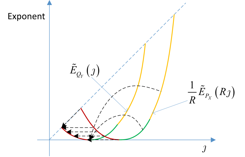
Figure 6: Illustration of the code used to prove the achievability for $\alpha\in[1,\infty]$ in Theorem 4 by using information spectrum exponents.

For this code, and for $0\leq s\leq 1$, we have (252)-(258) (given on page 252),

$$D_{1+s}(P_{Y^{n}}||Q_{Y}^{n}) =\frac{1}{s}\log\sum_{y^{n}}P_{Y^{n}}(y^{n})^{1+s}Q_{Y}^{n}(y^{n})^{-s}$$ (252)

$$\leq\frac{1}{s}\log\sum_{y^{n}}P_{Y^{n}}(y^{n})\Biggl{[}P_{X}^{k}(x_{i\left(y^{n}\right)}^{k})1\{P_{X}^{k}(x_{i\left(y^{n}\right)}^{k})\geq\widetilde{Q}_{Y^{n}}(y^{n})\}$$

$$\qquad+\left(\widetilde{Q}_{Y^{n}}(y^{n})+P_{X}^{k}(x_{i\left(y^{n}\right)}^{k})\right)1\{P_{X}^{k}(x_{i\left(y^{n}\right)}^{k})<\widetilde{Q}_{Y^{n}}(y^{n})\}\Biggr{]}^{s}Q_{Y}^{n}(y^{n})^{-s}$$ (253)

$$=\frac{1}{s}\log\sum_{y^{n}}P_{Y^{n}}(y^{n})\Biggl{[}\left(\frac{P_{X}^{k}(x_{i\left(y^{n}\right)}^{k})}{Q_{Y^{n}}(y^{n})}\right)^{s}1\{P_{X}^{k}(x_{i\left(y^{n}\right)}^{k})\geq\widetilde{Q}_{Y^{n}}(y^{n})\}$$

$$\qquad+\left(\frac{\widetilde{Q}_{Y^{n}}(y^{n})}{Q_{Y^{n}}(y^{n})}\right)^{s}\left(1+\frac{P_{X}^{k}(x_{i\left(y^{n}\right)}^{k})}{\widetilde{Q}_{Y^{n}}(y^{n})}\right)^{s}1\{P_{X}^{k}(x_{i\left(y^{n}\right)}^{k})<\widetilde{Q}_{Y^{n}}(y^{n})\}\Biggr{]}$$ (254)

$$\leq\frac{1}{s}\log\sum_{y^{n}}P_{Y^{n}}(y^{n})\Biggl{[}\left(\frac{P_{X}^{k}(x_{i\left(y^{n}\right)}^{k})}{Q_{Y^{n}}(y^{n})}\right)^{s}1\{P_{X}^{k}(x_{i\left(y^{n}\right)}^{k})\geq\widetilde{Q}_{Y^{n}}(y^{n})\}$$

$$\qquad+\left(\frac{\widetilde{Q}_{Y^{n}}(y^{n})}{Q_{Y^{n}}(y^{n})}\right)^{s}\left(1+\left(\frac{P_{X}^{k}(x_{i\left(y^{n}\right)}^{k})}{\widetilde{Q}_{Y^{n}}(y^{n})}\right)^{s}\right)1\{P_{X}^{k}(x_{i\left(y^{n}\right)}^{k})<\widetilde{Q}_{Y^{n}}(y^{n})\}\Biggr{]}$$ (255)

$$=\frac{1}{s}\log Q_{Y}^{n}(\mathcal{A})^{-s}\sum_{y^{n}}P_{Y^{n}}(y^{n})\left(\left(\frac{P_{X}^{k}(x_{i\left(y^{n}\right)}^{k})}{\widetilde{Q}_{Y^{n}}(y^{n})}\right)^{s}+1\{P_{X}^{k}(x_{i\left(y^{n}\right)}^{k})<\widetilde{Q}_{Y^{n}}(y^{n})\}\right)$$ (256)

$$\leq\frac{1}{s}\log Q_{Y}^{n}(\mathcal{A})^{-s}\sum_{y^{n}}P_{Y^{n}}(y^{n})\left(\left(\frac{P_{X}^{k}(x_{i\left(y^{n}\right)}^{k})}{\widetilde{Q}_{Y^{n}}(y^{n})}\right)^{s}+1\right)$$ (257)

$$\leq-\log Q_{Y}^{n}(\mathcal{A})+\frac{1}{s}Q_{Y}^{n}(\mathcal{A})^{-s}\sum_{y^{n}}P_{Y^{n}}(y^{n})\left(\frac{P_{X}^{k}(x_{i\left(y^{n}\right)}^{k})}{\widetilde{Q}_{Y^{n}}(y^{n})}\right)^{s}$$ (258)

where (255) follows from Lemma 6. To show $D_{1+s}(P_{Y^{n}}||Q_{Y}^{n})\to 0$, we only need to show both terms in (258) converge to zero. Obviously, the first term converges to zero since $Q_{Y}^{n}(\mathcal{A})\to 1$. Next we focus on the second term. We have (259)-(263) (given on page 259),

$$\sum_{y^{n}}P_{Y^{n}}(y^{n})\left(\frac{P_{X}^{k}(x_{i\left(y^{n}\right)}^{k})}{\widetilde{Q}_{Y^{n}}(y^{n})}\right)^{s}$$

$$\leq\sum_{y^{n}}\left(P_{Y^{n}}(y^{n})1\{P_{X}^{k}(x_{i\left(y^{n}\right)}^{k})\geq\widetilde{Q}_{Y^{n}}(y^{n})\}+\left(\widetilde{Q}_{Y^{n}}(y^{n})+P_{X}^{k}(x_{i\left(y^{n}\right)}^{k})\right)1\{P_{X}^{k}(x_{i\left(y^{n}\right)}^{k})<\widetilde{Q}_{Y^{n}}(y^{n})\}\right)\left(\frac{P_{X}^{k}(x_{i\left(y^{n}\right)}^{k})}{\widetilde{Q}_{Y^{n}}(y^{n})}\right)^{s}$$ (259)

$$\leq\sum_{y^{n}}\left(P_{Y^{n}}(y^{n})1\{P_{X}^{k}(x_{i\left(y^{n}\right)}^{k})\geq\widetilde{Q}_{Y^{n}}(y^{n})\}+2\widetilde{Q}_{Y^{n}}(y^{n})1\{P_{X}^{k}(x_{i\left(y^{n}\right)}^{k})<\widetilde{Q}_{Y^{n}}(y^{n})\}\right)\left(\frac{P_{X}^{k}(x_{i\left(y^{n}\right)}^{k})}{\widetilde{Q}_{Y^{n}}(y^{n})}\right)^{s}$$ (260)

$$\leq\sum_{x^{k}}P_{X}^{k}(x^{k})\left(\frac{P_{X}^{k}(x^{k})}{\widetilde{Q}_{Y^{n}}(y_{j(x^{k})}^{n})}\right)^{s}1\{P_{X}^{k}(x^{k})\geq\widetilde{Q}_{Y^{n}}(y_{j(x^{k})}^{n})\}+2\sum_{j=1}^{|\mathcal{A}|}\sum_{x^{k}\in\mathcal{B}_{j}}\frac{P_{X}^{k}(x^{k})}{\sum_{x^{n}\in\mathcal{B}_{j}}P_{X}^{k}(x^{k})}\widetilde{Q}_{Y^{n}}(y_{j}^{n})\left(\frac{P_{X}^{k}(x^{k})}{\widetilde{Q}_{Y^{n}}(y_{j}^{n})}\right)^{s}$$

$$\qquad\times 1\{P_{X}^{k}(x^{k})<\widetilde{Q}_{Y^{n}}(y_{j}^{n})\}$$ (261)

$$\leq\sum_{x^{k}}P_{X}^{k}(x^{k})\left(\frac{P_{X}^{k}(x^{k})}{\widetilde{Q}_{Y^{n}}(y_{j(x^{k})}^{n})}\right)^{s}1\{P_{X}^{k}(x^{k})\geq\widetilde{Q}_{Y^{n}}(y_{j(x^{k})}^{n})\}+4\sum_{x^{k}}P_{X}^{k}(x^{k})\left(\frac{P_{X}^{k}(x^{k})}{\widetilde{Q}_{Y^{n}}(y_{j(x^{k})}^{n})}\right)^{s}1\{P_{X}^{k}(x^{k})<\widetilde{Q}_{Y^{n}}(y_{j}^{n})\}$$ (262)

$$\leq 4\sum_{x^{k}}P_{X}^{k}(x^{k})\left(\frac{P_{X}^{k}(x^{k})}{\widetilde{Q}_{Y^{n}}(y_{j(x^{k})}^{n})}\right)^{s}$$ (263)

where $\mathcal{B}_{j}$ denotes the set of $x^{n}$ that are mapped to $y_{j}^{n}$, (261) follows since $P_{X}^{k}(x_{i\left(y^{n}\right)}^{k})\leq P_{X}^{k}(x^{k})$ for all $x^{n}$ that are mapped to $y^{n}$, and (262) follows since

$$\sum_{x^{k}\in\mathcal{B}_{j}}\frac{P_{X}^{k}(x^{k})}{\sum_{x^{k}\in\mathcal{B}_{j}}P_{X}^{k}(x^{k})}\widetilde{Q}_{Y^{n}}(y_{j}^{n})\left(\frac{P_{X}^{k}(x^{k})}{\widetilde{Q}_{Y^{n}}(y_{j}^{n})}\right)^{s}$$

$$=\sum_{x^{k}\in\mathcal{B}_{j}}\frac{P_{X}^{k}(x^{k})}{P_{Y^{n}}(y_{j}^{n})}\widetilde{Q}_{Y^{n}}(y_{j}^{n})\left(\frac{P_{X}^{k}(x^{k})}{\widetilde{Q}_{Y^{n}}(y_{j}^{n})}\right)^{s}$$ (264)

$$\leq\sum_{x^{k}\in\mathcal{B}_{j}}\frac{P_{X}^{k}(x^{k})}{\frac{1}{2}\widetilde{Q}_{Y^{n}}(y_{j}^{n})}\widetilde{Q}_{Y^{n}}(y_{j}^{n})\left(\frac{P_{X}^{k}(x^{k})}{\widetilde{Q}_{Y^{n}}(y_{j}^{n})}\right)^{s}$$ (265)

$$=2\sum_{x^{k}\in\mathcal{B}_{j}}P_{X}^{k}(x^{k})\left(\frac{P_{X}^{k}(x^{k})}{\widetilde{Q}_{Y^{n}}(y_{j}^{n})}\right)^{s}.$$ (266)

Next we prove $\sum_{x^{k}}P_{X}^{k}(x^{k})\left(\frac{P_{X}^{k}(x^{k})}{\widetilde{Q}_{Y^{n}}(y_{j(x^{k})}^{n})}\right)^{s}\to 0$.

Based on the notations defined in Appendix A-B, and using Lemma 9, we have

$$Q_{Y}^{n}\left(y_{j(x^{k})}^{n}\right)$$

$$=Q_{Y}^{n}\left(y_{G_{Y^{n}}^{-1}\left(G_{X^{k}}(i)\right)}^{n}\right)$$ (267)

$$\geq F_{Q_{Y}^{n}}^{-1}\left(F_{P_{X}^{k}}\left(-\frac{1}{k}\log P_{X}^{k}(x^{k})\right)\right)$$ (268)

$$=\exp\biggl{\{}-nE_{Q_{Y}}^{-1}\Bigl{(}-\frac{1}{n}\log\left\{e^{-k\left(E_{P_{X}}(-\frac{1}{k}\log P_{X}^{k}(x^{k}))+o(1)\right)}\right\}$$

$$\qquad+o(1)\Bigr{)}\biggr{\}}$$ (269)

$$=\exp\left\{-nE_{Q_{Y}}^{-1}\left(\frac{k}{n}\left(E_{P_{X}}(-\frac{1}{k}\log P_{X}^{k}(x^{k}))\right)+o(1)\right)\right\}$$ (270)

$$=\exp\Biggl{\{}-n\max_{t\in[0,\infty]}\biggl{\{}H_{1+t}(Q_{Y})-\frac{1}{t}$$

$$\times\left(\frac{k}{n}\max_{t^{\prime}\in[0,\infty]}\left\{t^{\prime}H_{1+t^{\prime}}(P_{X})+\frac{t^{\prime}}{k}\log P_{X}^{k}(x^{k})\right\}+o(1)\right)\biggr{\}}\Biggr{\}}$$ (271)

where $i$ (in (267)) denotes the index of $x^{n}$ in the sequence $x_{1}^{n},x_{2}^{n},...,x_{|\mathcal{X}|^{n}}^{n}$.

Therefore, we have (272)-(280) (given on page 272),

$$\limsup_{n\to\infty}\frac{1}{n}\log\sum_{x^{k}}P_{X}^{k}(x^{k})\left(\frac{P_{X}^{k}(x^{k})}{Q_{Y}^{n}(y_{j(x^{n})}^{n})}\right)^{s}$$

$$\leq\limsup_{n\to\infty}\frac{1}{n}\log\sum_{T_{X}}\sum_{x^{n}\in\mathcal{T}_{T_{X}}}e^{sn\max_{t\in[0,\infty]}\left\{H_{1+t}(Q_{Y})-\frac{1}{t}\left(\frac{k}{n}\max_{t^{\prime}\in[0,\infty]}\left\{t^{\prime}H_{1+t^{\prime}}(P_{X})+\frac{t^{\prime}}{k}\log P_{X}^{k}(x^{k})\right\}+o(1)\right)\right\}}$$

$$\qquad\times e^{\left(1+s\right)k\sum_{x}T_{X}(x)\log P_{X}(x)}$$ (272)

$$=\limsup_{n\to\infty}\max_{T_{X}}\frac{k}{n}\left(H(T_{X})+\left(1+s\right)\sum_{x}T_{X}(x)\log P_{X}(x)\right)$$

$$\qquad+s\max_{t\in[0,\infty]}\left\{H_{1+\frac{1}{t}}(Q_{Y})-t\left(\frac{k}{n}\max_{t^{\prime}\in[0,\infty]}\left\{t^{\prime}H_{1+t^{\prime}}(P_{X})+t^{\prime}\sum_{x}T_{X}(x)\log P_{X}(x)\right\}+o(1)\right)\right\}$$ (273)

$$=\limsup_{n\to\infty}\max_{\widetilde{P}_{X}\in\mathcal{P}\left(\mathcal{X}\right)}\frac{k}{n}\left(H(\widetilde{P}_{X})+\left(1+s\right)\sum_{x}\widetilde{P}_{X}(x)\log P_{X}(x)\right)$$

$$\qquad+s\max_{t\in[0,\infty]}\left\{H_{1+\frac{1}{t}}(Q_{Y})-t\left(\frac{k}{n}\max_{t^{\prime}\in[0,\infty]}\left\{t^{\prime}H_{1+t^{\prime}}(P_{X})+t^{\prime}\sum_{x}\widetilde{P}_{X}(x)\log P_{X}(x)\right\}+o(1)\right)\right\}$$ (274)

$$=\max_{\widetilde{P}_{X}\in\mathcal{P}\left(\mathcal{X}\right)}\frac{1}{R}\left(H(\widetilde{P}_{X})+\left(1+s\right)\sum_{x}\widetilde{P}_{X}(x)\log P_{X}(x)\right)$$

$$\qquad+s\max_{t\in[0,\infty]}\left\{H_{1+\frac{1}{t}}(Q_{Y})-\frac{t}{R}\max_{t^{\prime}\in[0,\infty]}\left\{t^{\prime}H_{1+t^{\prime}}(P_{X})+t^{\prime}\sum_{x}\widetilde{P}_{X}(x)\log P_{X}(x)\right\}\right\}$$ (275)

$$\leq\max_{t\in[0,\infty]}\min_{t^{\prime}\in[0,\infty]}\max_{\widetilde{P}_{X}\in\mathcal{P}\left(\mathcal{X}\right)}\frac{1}{R}\left(H(\widetilde{P}_{X})+\left(1+s\right)\sum_{x}\widetilde{P}_{X}(x)\log P_{X}(x)\right)$$ (276)

$$\qquad+s\left\{H_{1+\frac{1}{t}}(Q_{Y})-\frac{t}{R}\left\{t^{\prime}H_{1+t^{\prime}}(P_{X})+t^{\prime}\sum_{x}\widetilde{P}_{X}(x)\log P_{X}(x)\right\}\right\}$$ (277)

$$=\max_{t\in[0,\infty]}\min_{t^{\prime}\in[0,\infty]}-\frac{s}{R}H_{1+s-stt^{\prime}}(P_{X})+sH_{1+\frac{1}{t}}(Q_{Y})-\frac{stt^{\prime}}{R}\left(H_{1+t^{\prime}}(P_{X})-H_{1+s-stt^{\prime}}(P_{X})\right)$$ (278)

$$\leq\max_{t\in[0,\infty]}-\frac{s}{R}H_{1+\frac{s}{1+st}}(P_{X})+sH_{1+\frac{1}{t}}(Q_{Y})$$ (279)

$$=\max_{t^{\prime\prime}\in[0,1]}\left\{sH_{\frac{1}{1-t^{\prime\prime}}}(Q_{Y})-\frac{s}{R}H_{\frac{t^{\prime\prime}+s}{t^{\prime\prime}+s-st^{\prime\prime}}}(P_{X})\right\}$$ (280)

where (275) follows from Lemma 9, and (279) follows by choosing $t^{\prime}=\frac{s}{1+st}$.

Therefore, if

$$R<\min_{t^{\prime\prime}\in[0,1]}\frac{H_{\frac{t^{\prime\prime}+s}{t^{\prime\prime}+s-st^{\prime\prime}}}(P_{X})}{H_{\frac{1}{1-t^{\prime\prime}}}(Q_{Y})}$$ (281)

then

$$\limsup_{n\to\infty}\frac{1}{n}\log\sum_{x^{k}}P_{X}^{k}(x^{k})\left(\frac{P_{X}^{k}(x^{k})}{Q_{Y}^{n}(y_{j(x^{k})}^{n})}\right)^{s}<0.$$ (282)

Hence $\sum_{x^{k}}P_{X}^{k}(x^{k})\left(\frac{P_{X}^{k}(x^{k})}{Q_{Y}^{n}(y_{j(x^{k})}^{n})}\right)^{s}\to 0$. This completes the proof for $0\leq s\leq 1$. For other $s$, it can be proven similarly (by other inequalities in Lemma 6).

Appendix F Proof of Theorem 5

The equality in (36) follows from Theorem 2. For (37), the case $\alpha=0$ can be proven easily. The cases $\alpha\in(0,1]\cup\left\{\infty\right\}$ follow by showing the achievability parts for $\alpha=1$ and $\alpha=\infty$. Next we prove these.

Here we assume that both $P_{X}$ and $Q_{Y}$ are not uniform. The cases that $P_{X}$ is uniform or $Q_{Y}$ is uniform will be proven in Theorems 8 and 11, respectively.

Achievability part for $\alpha=1$: Define

$$\mathcal{A} :=\left\{x^{k}:e^{-k\left(H(P_{X})+\delta\right)}\leq P_{X}^{k}(x^{k})\leq e^{-k\left(H(P_{X})-\delta\right)}\right\}$$ (283)

$$\mathcal{B} :=\left\{y^{n}:e^{-n\left(H(Q_{Y})+\delta\right)}\leq Q_{Y}^{n}(y^{n})\leq e^{-n\left(H(Q_{Y})-\delta\right)}\right\}.$$ (284)

Here $\delta>0$ is a number such that $H(P_{X})+\delta<H_{0}(P_{X})$ and $\frac{1}{R}\left(H(P_{X})-\delta\right)>H(Q_{Y})+\delta$. We consider the following mapping.

1. Map the sequences in $\mathcal{A}^{c}$ to the sequences in $\mathcal{B}^{c}$ such that for each $y^{n}\in\mathcal{B}^{c}$, there exists at least one $x^{n}\in\mathcal{A}^{c}$ mapped to it. This is feasible since

   $$\liminf_{n\to\infty}\frac{1}{n}\log\left|\mathcal{A}^{c}\right|$$

   $$=\liminf_{n\to\infty}\frac{1}{n}\log\left(\left|\mathcal{X}\right|^{k}-\left|\mathcal{A}\right|\right)$$ (285)

   $$\geq\liminf_{n\to\infty}\frac{1}{n}\log\left(e^{kH_{0}(P_{X})}-e^{k\left(H(P_{X})+\delta\right)}\right)$$ (286)

   $$=\frac{H_{0}(P_{X})}{R}$$ (287)

   $$>H_{0}(Q_{Y})$$ (288)

   $$\geq\limsup_{n\to\infty}\frac{1}{n}\log\left|\mathcal{B}^{c}\right|,$$ (289)

   i.e., $\left|\mathcal{A}^{c}\right|>\left|\mathcal{B}^{c}\right|$ for sufficiently large $n$.

2. Use Mapping 1 given in Appendix I-E to map the sequences in $\mathcal{A}$ to the sequences in $\mathcal{B}$, where the distributions $P_{X}$ and $Q_{Y}$ are respectively replaced by $\frac{P_{X}^{k}(x^{k})1\left\{x^{k}\in\mathcal{A}\right\}}{P_{X}^{k}(\mathcal{A})}$ and $\frac{Q_{Y}^{n}(y^{n})1\left\{y^{n}\in\mathcal{B}\right\}}{Q_{Y}^{n}(\mathcal{B})}$. Observe that $\frac{1}{R}\left(H(P_{X})-\delta\right)>H(Q_{Y})+\delta$ implies that $\frac{P_{X}^{k}(x^{k})}{P_{X}^{k}(\mathcal{A})}\leq\frac{Q_{Y}^{n}(y^{n})}{Q_{Y}^{n}(\mathcal{B})}$ for $x^{k}\in\mathcal{A},y^{n}\in\mathcal{B}$ and sufficiently large $n$. Hence by the property of Mapping 1, for $m\in[1:|\mathcal{B}|]$, $\frac{P_{X}^{k}(\mathcal{A})Q_{Y}^{n}(y_{m}^{n})}{Q_{Y}^{n}(\mathcal{B})}-P_{X}^{k}(x_{k_{m}}^{k})\leq P_{Y^{n}}(y_{m}^{n})\leq\frac{P_{X}^{k}(\mathcal{A})Q_{Y}^{n}(y_{m}^{n})}{Q_{Y}^{n}(\mathcal{B})}+P_{X}^{k}(x_{k_{m}}^{k})$. By the asymptotic equipartition property [29], we know that this step can be roughly considered as mapping a uniform distribution (with a larger alphabet) to another one (with a smaller alphabet).

For this code, and for sufficiently large $n$, we have

$$D(Q_{Y}^{n}\|P_{Y^{n}})$$

$$=\sum_{y^{n}\in\mathcal{B}}Q_{Y}^{n}(y^{n})\log\frac{Q_{Y}^{n}(y^{n})}{P_{Y^{n}}(y^{n})}+\sum_{y^{n}\in\mathcal{B}^{c}}Q_{Y}^{n}(y^{n})\log\frac{Q_{Y}^{n}(y^{n})}{P_{Y^{n}}(y^{n})}$$ (290)

$$\leq\sum_{m\in[1:|\mathcal{B}|]}Q_{Y}^{n}(y_{m}^{n})\log\frac{Q_{Y}^{n}(y_{m}^{n})}{\frac{P_{X}^{k}(\mathcal{A})Q_{Y}^{n}(y_{m}^{n})}{Q_{Y}^{n}(\mathcal{B})}-P_{X}^{k}(x_{k_{m}}^{k})}$$

$$\qquad+\sum_{y^{n}\in\mathcal{B}^{c}}Q_{Y}^{n}(y^{n})\log\frac{\left(\max_{y}Q_{Y}(y)\right)^{n}}{\left(\min_{x}P_{X}(x)\right)^{k}}$$ (291)

$$=-\sum_{m\in[1:|\mathcal{B}|]}Q_{Y}^{n}(y_{m}^{n})\log\left(\frac{P_{X}^{k}(\mathcal{A})}{Q_{Y}^{n}(\mathcal{B})}-\frac{P_{X}^{k}(x_{k_{m}}^{k})}{Q_{Y}^{n}(y_{m}^{n})}\right)$$

$$\qquad+nQ_{Y}^{n}(\mathcal{B}^{c})\log\frac{\max_{y}Q_{Y}(y)}{\left(\min_{x}P_{X}(x)\right)^{\frac{1}{R}}}$$ (292)

$$\leq-Q_{Y}^{n}(\mathcal{B})\log\left(\frac{P_{X}^{k}(\mathcal{A})}{Q_{Y}^{n}(\mathcal{B})}-\max_{m\in[1:|\mathcal{B}|]}\frac{P_{X}^{k}(x_{k_{m}}^{k})}{Q_{Y}^{n}(y_{m}^{n})}\right)$$

$$\qquad+nQ_{Y}^{n}(\mathcal{B}^{c})\log\frac{\max_{y}Q_{Y}(y)}{\left(\min_{x}P_{X}(x)\right)^{\frac{1}{R}}}$$ (293)

$$\leq-Q_{Y}^{n}(\mathcal{B})\log\left(\frac{P_{X}^{k}(\mathcal{A})}{Q_{Y}^{n}(\mathcal{B})}-e^{-n\left(\frac{1}{R}\left(H(P_{X})-\delta\right)-\left(H(Q_{Y})+\delta\right)\right)}\right)$$

$$\qquad+nQ_{Y}^{n}(\mathcal{B}^{c})\log\frac{\max_{y}Q_{Y}(y)}{\left(\min_{x}P_{X}(x)\right)^{\frac{1}{R}}}$$ (294)

$$\rightarrow 0$$ (295)

where (295) follows from $\frac{1}{R}\left(H(P_{X})-\delta\right)>H(Q_{Y})+\delta$ and the fact $P_{X}^{n}(\mathcal{A}^{c}),Q_{Y}^{n}(\mathcal{B}^{c})\rightarrow 0$ exponentially fast, as shown in the following inequalities.

$$Q_{Y}^{n}(\mathcal{B}^{c}) =\sum_{y^{n}\in\mathcal{B}^{c}}Q_{Y}^{n}(y^{n})$$ (296)

$$=Q_{Y}^{n}\left\{y^{n}:-\frac{1}{n}\log Q_{Y}^{n}(y^{n})<H(Q_{Y})+\delta\right\}$$

$$\qquad+Q_{Y}^{n}\left\{y^{n}:-\frac{1}{n}\log Q_{Y}^{n}(y^{n})>H(Q_{Y})-\delta\right\}$$ (297)

$$\doteq e^{-nE_{Q_{Y}}(H(Q_{Y})-\delta)}+e^{-n\widehat{E}_{Q_{Y}}(H(Q_{Y})+\delta)}$$

$$\doteq e^{-nE},$$ (298)

where

$$E:=\min\left\{E_{Q_{Y}}(H(Q_{Y})-\delta),\widehat{E}_{Q_{Y}}(H(Q_{Y})+\delta)\right\}>0.$$ (299)

Achievability part for $\alpha=\infty$: Partition $\mathcal{X}{}^{k}$ into four parts:

$$\mathcal{A}_{1}:=\left\{x^{k}:P_{X}^{k}(x^{k})>e^{-k\left(H(P_{X})-\delta\right)}\right\},$$ (300)

$$\mathcal{A}_{2}:=\left\{x^{k}:e^{-k\left(H^{\mathrm{u}}(P_{X})-\delta\right)}<P_{X}^{k}(x^{k})\leq e^{-k\left(H(P_{X})-\delta\right)}\right\},$$ (301)

$$\mathcal{A}_{3}:=\left\{x^{k}:e^{-kH^{\mathrm{u}}(P_{X})}\leq P_{X}^{k}(x^{k})\leq e^{-k\left(H^{\mathrm{u}}(P_{X})-\delta\right)}\right\},$$ (302)

$$\mathcal{A}_{4}:=\left\{x^{k}:P_{X}^{k}(x^{k})<e^{-kH^{\mathrm{u}}(P_{X})}\right\}.$$ (303)

Define $E^{*}:=\widehat{E}_{Q_{Y}}^{-1}\left(\frac{1}{R}\left(\widehat{E}_{P_{X}}(H^{\mathrm{u}}(P_{X}))\right)\right)$. Partition $\mathcal{Y}^{n}$ into two parts:

$$\mathcal{B}_{1}:=\left\{y^{n}:Q_{Y}^{n}\left(y^{n}\right)\geq e^{-nE^{*}}\right\}$$ (304)

$$\mathcal{B}_{2}:=\left\{y^{n}:Q_{Y}^{n}\left(y^{n}\right)<e^{-nE^{*}}\right\}.$$ (305)

Consider the following code. This code is illustrated in Fig. 7.

1. Map the sequences in $\mathcal{A}_{1}\cup\mathcal{A}_{4}$ to those in $\mathcal{Y}^{n}$ in any way.

2. Use Mapping 1 given in Appendix I-E to map the sequences in $\mathcal{A}_{2}$ to the sequences in $\mathcal{B}_{1}$.

3. Use Mapping 2 given in Appendix I-E to map the sequences in $\mathcal{A}_{3}$ to the sequences in $\mathcal{B}_{2}$.

Figure 7: Illustration of the code used to prove the achievability for $\alpha=\infty$ in Theorem 5 by using information spectrum exponents.

Assume

$$R<\min_{t\in[0,\infty]}\frac{H_{\frac{1}{1+t}}(P_{X})}{H_{\frac{1}{1+t}}(Q_{Y})}.$$ (306)

By Lemma 11, we have

$$\frac{1}{R}\widehat{E}_{P_{X}}(R\jmath) <\widehat{E}_{Q_{Y}}(\jmath),\>\forall\jmath\in\frac{1}{R}[H(P_{X}),H^{\mathrm{u}}(P_{X})]$$ (307)

$$R <\frac{H_{0}(P_{X})}{H_{0}(Q_{Y})}.$$ (308)

We first prove $\log\max_{y^{n}\in\mathcal{B}_{1}}\frac{Q_{Y}^{n}(y^{n})}{P_{Y^{n}}(y^{n})}\rightarrow 0.$ Observe that $P_{X}^{k}(\mathcal{A}_{2}),Q_{Y}^{n}\left(\mathcal{B}_{1}\right)\to 1$ as $n\to\infty$. Define $\widetilde{P}_{X^{k}}\left(x^{k}\right):=\frac{P_{X}^{k}(x^{k})1\left\{x^{k}\in\mathcal{A}_{2}\right\}}{P_{X}^{k}(\mathcal{A}_{2})}$ and $\widetilde{Q}_{Y^{n}}\left(y^{n}\right):=\frac{Q_{Y}^{n}(y^{n})1\left\{y^{n}\in\mathcal{B}_{1}\right\}}{Q_{Y}^{n}(\mathcal{B}_{1})}$. To prove $\log\max_{j\in\mathcal{B}_{1}}\frac{Q_{Y}^{n}(y_{j}^{n})}{P_{Y^{n}}(y_{j}^{n})}\rightarrow 0$, we only need to prove $\log\max_{y^{n}\in\mathcal{B}_{1}}\frac{Q_{Y}^{n}(y^{n})}{P_{Y^{n}}(y^{n})}\rightarrow 0$, where $\widetilde{P}_{Y^{n}}(y^{n}):=\frac{P_{Y^{n}}(y^{n})}{P_{X}^{k}(\mathcal{A}_{2})}$. Define $\mathcal{J}_{1}:=\frac{1}{R}[H(P_{X})-\delta,H(P_{X}))$ and $\mathcal{J}_{2}:=\frac{1}{R}[H(P_{X}),H^{\mathrm{u}}(P_{X})-\delta)$. Then for $\jmath\in\mathcal{J}_{2}$, we have that

$$\lim_{k\to\infty}-\frac{1}{k}\log\left(1-F_{\widetilde{P}_{X^{k}}}(\jmath)\right)$$

$$=\lim_{k\to\infty}-\frac{1}{k}\log\widetilde{P}_{X^{k}}\left(x^{k}:-\frac{1}{k}\log\widetilde{P}_{X^{k}}(x^{k})\geq\jmath\right)$$ (309)

$$=\lim_{k\to\infty}-\frac{1}{k}\log\frac{P_{X}^{k}\left(x^{k}\in\mathcal{A}_{2}:-\frac{1}{k}\log\frac{P_{X}^{k}(x^{k})}{P_{X}^{k}(\mathcal{A}_{2})}\geq\jmath\right)}{P_{X}^{k}(\mathcal{A}_{2})}$$ (310)

$$=\lim_{k\to\infty}-\frac{1}{k}\log P_{X}^{k}\left(x^{k}\in\mathcal{A}_{2}:-\frac{1}{k}\log P_{X}^{k}(x^{k})\geq\jmath+o(1)\right)$$ (311)

$$=\widehat{E}_{P_{X}}(\jmath),$$ (312)

where (312) follows from Lemma 12. Similarly, for $\jmath\in[H_{\infty}(Q_{Y}),E^{*})$,

$$\lim_{n\to\infty}-\frac{1}{n}\log\left(1-F_{\widetilde{Q}_{Y^{n}}}(\jmath)\right)=\widehat{E}_{Q_{Y}}(\jmath),$$ (313)

Observe that by Lemma 9, $\widehat{E}_{Q_{Y}}(\jmath)$ is continuous. Hence (307) implies that there exists some $\epsilon>0$ such that for any $\jmath\in\mathcal{J}_{2}$,

$$\frac{1}{R}\widehat{E}_{P_{X}}(R\jmath)\leq\widehat{E}_{Q_{Y}}(\jmath-\epsilon)-\epsilon.$$ (314)

i.e.,

$$\limsup_{n\to\infty}\frac{1}{n}\log\sup_{\jmath\in\mathcal{J}_{2}}\frac{1-F_{\widetilde{Q}_{Y^{n}}}(\jmath-\epsilon)}{1-F_{\widetilde{P}_{X^{k}}}(R\jmath)} \leq-\epsilon.$$ (315)

or equivalently,

$$\liminf_{n\to\infty}\inf_{\theta\in F_{\widetilde{P}_{X^{k}}}(R\mathcal{J}_{2})}\left\{\frac{1}{R}F_{\widetilde{P}_{X^{k}}}^{-1}(\theta)-F_{\widetilde{Q}_{Y^{n}}}^{-1}(1-(1-\theta)e^{-n\epsilon})\right\}$$

$$\geq\epsilon.$$ (316)

Since $F_{\widetilde{Q}_{Y^{n}}}^{-1}(\theta)$ is nonincreasing in $\theta$, (316) implies

$$\liminf_{n\to\infty}\inf_{\theta\in F_{\widetilde{P}_{X^{k}}}(R\mathcal{J}_{2})}\left\{\frac{1}{R}F_{\widetilde{P}_{X^{k}}}^{-1}(\theta)-F_{\widetilde{Q}_{Y^{n}}}^{-1}(\theta)\right\} \geq\epsilon.$$ (317)

On the other hand, by choosing $\delta>0$ small enough, we have $H(Q_{Y})<\frac{1}{R}(H(P_{X})-\delta)$. This implies that for some $\epsilon>0$,

$$\liminf_{n\to\infty}\inf_{\theta\in F_{\widetilde{P}_{X^{k}}}(R\mathcal{J}_{1})}\left\{\frac{1}{R}F_{\widetilde{P}_{X^{k}}}^{-1}(\theta)-F_{\widetilde{Q}_{Y^{n}}}^{-1}(\theta)\right\} \geq\epsilon.$$ (318)

Combining (317) and (318) gives us that for some $\epsilon>0$,

$$\liminf_{n\to\infty}\inf_{\theta\in F_{\widetilde{P}_{X^{k}}}(R\left(\mathcal{J}_{1}\cup\mathcal{J}_{2}\right))}\left\{\frac{1}{R}F_{\widetilde{P}_{X^{k}}}^{-1}(\theta)-F_{\widetilde{Q}_{Y^{n}}}^{-1}(\theta)\right\} \geq\epsilon.$$ (319)

Observe that $F_{\widetilde{P}_{X^{k}}}^{-1}(\theta)$ is finite, hence (317) also holds if $R$ is replaced with $\frac{n}{k}$. Furthermore, similarly in Subsection I-E, we sort the elements in $\mathcal{A}_{2}$ as $x_{1}^{k},x_{2}^{k},...,x_{|\mathcal{A}_{2}|}^{k}$ such that $\widetilde{P}_{X^{k}}(x_{1}^{k})\geq\widetilde{P}_{X^{k}}(x_{2}^{k})\geq...\geq\widetilde{P}_{X^{k}}(x_{|\mathcal{A}_{2}|}^{k})$. Define $\widetilde{G}_{X^{k}}(i):=\widetilde{P}_{X^{k}}\left(x_{l}^{k}:l\leq i\right)$ and $\widetilde{G}_{X^{k}}^{-1}(\theta):=\max\left\{i\in\mathbb{N}:\widetilde{G}_{X^{k}}(i)\leq\theta\right\}$. Similarly, for $\widetilde{Q}_{Y^{n}}$, we define $\widetilde{G}_{Y^{n}}(j):=\widetilde{Q}_{Y^{n}}\left(y_{l}^{n}:l\leq j\right)$ and $\widetilde{G}_{Y^{n}}^{-1}(\theta):=\min\left\{j\in\mathbb{N}:\widetilde{G}_{Y^{n}}(j)\geq\theta\right\}$. Hence the mapping used here is $j=\widetilde{G}_{Y^{n}}^{-1}(\widetilde{G}_{X^{k}}(i))$. For each $i\in[1:|\mathcal{A}_{2}|]$, $\widetilde{G}_{X^{k}}(i)\in F_{\widetilde{P}_{X^{k}}}(\mathcal{J})$. Hence we have

$$\liminf_{n\to\infty}\min_{i\in[1:|\mathcal{A}_{2}|]}\frac{1}{n}\log\frac{\widetilde{Q}_{Y^{n}}(y_{j}^{n})}{\widetilde{P}_{X^{k}}(x_{i}^{k})}$$

$$=\liminf_{n\to\infty}\min_{i\in[1:|\mathcal{A}_{2}|]}\left\{\frac{k}{n}F_{\widetilde{P}_{X^{k}}}^{-1}(\widetilde{G}_{X^{k}}(i))-F_{\widetilde{Q}_{Y^{n}}}^{-1}(\widetilde{G}_{X^{k}}(i))\right\}$$ (320)

$$\geq\liminf_{n\to\infty}\inf_{\theta\in F_{\widetilde{P}_{X^{k}}}(R\left(\mathcal{J}_{1}\cup\mathcal{J}_{2}\right))}\left\{\frac{k}{n}F_{\widetilde{P}_{X^{k}}}^{-1}(\theta)-F_{\widetilde{Q}_{Y^{n}}}^{-1}(\theta)\right\}$$ (321)

$$\geq\epsilon,$$ (322)

where $j=\widetilde{G}_{Y^{n}}^{-1}(\widetilde{G}_{X^{k}}(i))$. Hence $\frac{\widetilde{Q}_{Y^{n}}(y_{j}^{n})}{\widetilde{P}_{X^{k}}(x_{i}^{k})}\to 0$ for any $i\in[1:|\mathcal{A}_{2}|]$. Therefore, we have

$$\log\max_{j\in[1:|\mathcal{B}_{1}|]}\frac{\widetilde{Q}_{Y^{n}}(y_{j}^{n})}{\widetilde{P}_{Y^{n}}(y_{j}^{n})}$$

$$\leq\log\max_{j\in[1:|\mathcal{B}_{1}|]}\frac{\widetilde{Q}_{Y^{n}}(y_{j}^{n})}{\widetilde{Q}_{Y^{n}}(y_{j}^{n})-\max_{i:\widetilde{G}_{Y^{n}}^{-1}(\widetilde{G}_{X^{k}}(i))=j}\widetilde{P}_{X^{k}}(x_{i}^{k})}$$ (323)

$$\rightarrow 0.$$ (324)

Hence $\log\max_{y^{n}\in\mathcal{B}_{1}}\frac{Q_{Y}^{n}(y^{n})}{P_{Y^{n}}(y^{n})}\rightarrow 0.$

We next prove $\log\max_{y^{n}\in\mathcal{B}_{2}}\frac{Q_{Y}^{n}(y^{n})}{P_{Y^{n}}(y^{n})}\leq 0.$ Observe that

$$\lim_{n\to\infty}-\frac{1}{n}\log Q_{Y}^{n}(\mathcal{B}_{2}) =\frac{1}{R}\left(\widehat{E}_{P_{X}}(H^{\mathrm{u}}(P_{X}))\right)$$ (325)

$$=\frac{1}{R}D(\mathrm{Unif}\left(\mathcal{X}\right)\|P_{X}),$$ (326)

$$\lim_{n\to\infty}-\frac{1}{n}\log\left(|\mathcal{Y}|^{n}p_{0}\right)$$

$$=\frac{1}{R}H^{\mathrm{u}}(P_{X})-H_{0}(Q_{Y})$$ (327)

$$=\frac{1}{R}H_{0}(P_{X})+\frac{1}{R}D(\mathrm{Unif}\left(\mathcal{X}\right)\|P_{X})-H_{0}(Q_{Y})$$ (328)

$$>\frac{1}{R}D(\mathrm{Unif}\left(\mathcal{X}\right)\|P_{X}),$$ (329)

and

$$\lim_{n\to\infty}\frac{1}{n}\log P_{X}^{k}(\mathcal{A}_{3}) =\frac{1}{R}\left(\widehat{E}_{P_{X}}(H^{\mathrm{u}}(P_{X})-\delta)\right)$$ (330)

$$<\frac{1}{R}D(\mathrm{Unif}\left(\mathcal{X}\right)\|P_{X}).$$ (331)

Hence for sufficiently large $n$, it holds that

$$Q_{Y}^{n}(\mathcal{B}_{2})+|\mathcal{Y}|^{n}p_{0}\leq P_{X}^{k}(\mathcal{A}_{3}),$$ (332)

which implies that by Mapping 2, $Q_{Y}^{n}(y^{n})\leq P_{Y^{n}}(y^{n})$ for $y^{n}\in\mathcal{B}_{2}$. That is, $\log\max_{y^{n}\in\mathcal{B}_{2}}\frac{Q_{Y}^{n}(y^{n})}{P_{Y^{n}}(y^{n})}\leq 0.$

Appendix G Proof of Theorem 6

By the equality $D_{\alpha}(Q\|P)=\frac{\alpha}{1-\alpha}D_{1-\alpha}(P\|Q)$ for $\alpha\in(0,1)$, the case $\alpha\in(0,1)$ has been proven in Theorem 4. Furthermore, it is easy to verify that the mapping used to prove for case $\alpha=0$ in Theorem 4 also satisfies $D_{0}(Q_{Y}^{n}\|P_{Y^{n}})\rightarrow 0$. So this proves the case $\alpha=0$. The case $\alpha=1$ can be proven by a proof similar to that in Appendix F. In the following, we consider the case $\alpha=\infty$.

We first prove the following bounds for the normalized and unnormalized Rényi conversion rates for general simulation problem (the seed and target distributions are not limited to product distributions). For general distributions $P_{X^{n}}$ and $Q_{Y^{n}}$, we use $P_{X^{n}}$ to approximate $Q_{Y^{n}}$. Define $F_{P_{X^{k}}}(\jmath):=P_{X^{k}}\left(x^{k}:-\frac{1}{k}\log P_{X^{k}}(x^{k})<\jmath\right)$ and $F_{P_{X^{k}}}^{-1}(\theta):=\sup\left\{\jmath:F_{P_{X^{k}}}(\jmath)\leq\theta\right\}$. For $Q_{Y^{n}}$, we define $F_{Q_{Y^{n}}}$ and $F_{Q_{Y^{n}}}^{-1}$ similarly. Then we have the following bounds.

Lemma 13.

$$\sup\biggl{\{}R:\sup_{\epsilon>0}\limsup_{n\to\infty}\frac{1}{n}\log\sup_{\jmath\geq 0}\frac{F_{P_{X^{k}}}(\frac{n}{k}(\jmath-\epsilon))}{F_{Q_{Y^{n}}}(\jmath)}\leq 0,$$

$$\qquad\sup_{\epsilon>0}\limsup_{n\to\infty}\frac{1}{n}\log\sup_{\jmath\geq 0}\frac{1-F_{Q_{Y^{n}}}(\jmath)}{1-F_{P_{X^{k}}}(\frac{n}{k}(\jmath-\epsilon))}\leq 0\biggr{\}}$$

$$\geq\sup\left\{R:\frac{1}{n}D_{\infty}^{\mathsf{max}}(P_{Y^{n}},Q_{Y^{n}})\rightarrow 0\right\}$$ (333)

$$\geq\sup\left\{R:D_{\infty}^{\mathsf{max}}(P_{Y^{n}},Q_{Y^{n}})\rightarrow 0\right\}$$ (334)

$$\geq\sup\left\{R:\liminf_{n\to\infty}\inf_{\theta\in[0,1)}\left\{\frac{k}{n}F_{P_{X^{k}}}^{-1}(\theta)-F_{Q_{Y^{n}}}^{-1}(\theta)\right\}>0\right\}.$$ (335)

Remark 21.

The upper bound can be rewritten as

$$\sup\biggl{\{}R:$$

$$\inf_{\epsilon>0}\liminf_{n\to\infty}\inf_{\theta\in[0,e^{-n\epsilon})}\left\{\frac{k}{n}F_{P_{X^{k}}}^{-1}(\theta e^{n\epsilon})-F_{Q_{Y^{n}}}^{-1}(\theta)\right\}\geq 0,$$

$$\inf_{\epsilon>0}\liminf_{n\to\infty}\inf_{\theta\in[0,1)}\left\{\frac{k}{n}F_{P_{X^{k}}}^{-1}(1-\left(1-\theta\right)e^{-n\epsilon})-F_{Q_{Y^{n}}}^{-1}(\theta)\right\}$$

$$\qquad\geq 0\biggr{\}},$$ (336)

and the lower bound can be further lower bounded by

$$\sup\biggl{\{}R:\inf_{\epsilon>0}\limsup_{n\to\infty}\sup_{\jmath\geq 0}\left\{F_{P_{X^{k}}}(\frac{n}{k}(\jmath+\epsilon))-F_{Q_{Y^{n}}}(\jmath)\right\}$$

$$\qquad<0\biggr{\}}.$$ (337)

Similar expressions for bounds on the conversion rate under the TV distance measure can be found in [30].

Remark 22.

By similar proofs, one can show a better upper bound and a better lower bound for the unnormalized Rényi conversion rate.

$$\sup\biggl{\{}R:\sup_{\epsilon>0}\limsup_{n\to\infty}\sup_{\jmath\geq 0}\left\{F_{P_{X^{k}}}(\frac{n}{k}(\jmath-\epsilon))-F_{Q_{Y^{n}}}(\jmath)\right\}$$

$$\qquad\leq 0\biggr{\}}$$

$$\geq\sup\left\{R:D_{\infty}^{\mathsf{max}}(P_{Y^{n}},Q_{Y}^{n})\rightarrow 0\right\}$$ (338)

$$\geq\sup\left\{R:\liminf_{n\to\infty}\inf_{\theta\in[0,1)}\left\{kF_{P_{X^{k}}}^{-1}(\theta)-nF_{Q_{Y^{n}}}^{-1}(\theta)\right\}=\infty\right\}.$$ (339)

Proof:

Achievability (Lower Bound): If $\liminf_{n\to\infty}\inf_{\theta\in[0,1)}\left\{\frac{k}{n}F_{P_{X^{k}}}^{-1}(\theta)-F_{Q_{Y^{n}}}^{-1}(\theta)\right\}>0$, then there exists a sufficiently small $\epsilon>0$ and a sufficiently large $K$ such that $\frac{k}{n}F_{P_{X^{k}}}^{-1}(\theta)-F_{Q_{Y^{n}}}^{-1}(\theta)>0$ for any $\theta\in[0,1)$ and for any $k\geq K$. Assume $x_{1}^{k},x_{2}^{k},...,x_{|\mathcal{X}|^{k}}^{k}$ is a sequence such that $P_{X^{k}}(x_{1}^{k})\geq P_{X^{k}}(x_{2}^{k})\geq...\geq P_{X^{k}}(x_{|\mathcal{X}|^{k}}^{k})$. Define $G_{X^{k}}(i)=P_{X^{k}}\left(x_{l}^{k}:l\leq i\right)$ and $G_{X^{k}}^{-1}(\theta):=\max\left\{i\in\mathbb{N}:F_{X^{k}}(i)\leq\theta\right\}$. Similarly, for $Q_{Y^{n}}$, we define $G_{Y^{n}}(j):=Q_{Y^{n}}\left(y_{l}:l\leq j\right)$ and $G_{Y^{n}}^{-1}:=\min\left\{j\in\mathbb{N}:G_{Y}(j)\geq\theta\right\}$. Use Mapping 1 given in Appendix I-E to map the sequences in $\mathcal{X}^{k}$ to the sequences in $\mathcal{Y}^{n}$, where the distributions $P_{X}$ and $Q_{Y}$ are respectively replaced by $P_{X^{k}}$ and $Q_{Y^{n}}$. That is, for each $i\in[1:|\mathcal{X}|^{k}]$, $x_{i}^{k}$ is mapped to $y_{j}^{n}$ where $j=G_{Y^{n}}^{-1}(G_{X^{k}}(i))$. This code is illustrated in Fig. 8.

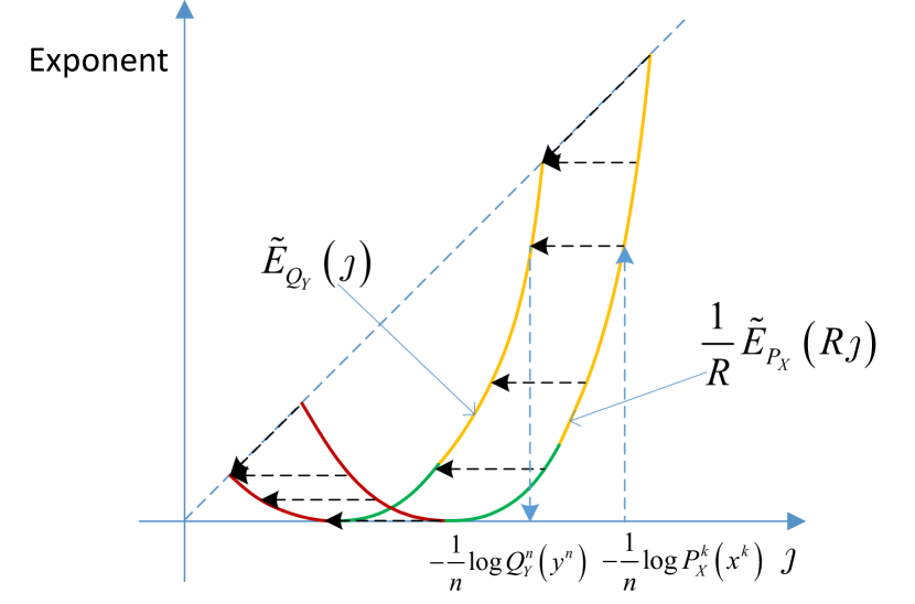
Figure 8: Illustration of the code used to prove the achievability for $\alpha=\infty$ in Theorem 6 (or Lemma 13) by using information spectrum exponents.

Hence for each $j\in[1:|\mathcal{Y}|^{n}]$,

$$Q_{Y^{n}}(y_{j}^{n})-P_{X^{k}}(x_{i}^{k})\leq P_{Y^{n}}(y_{j}^{n})\leq Q_{Y^{n}}(y_{j}^{n})+P_{X^{k}}(x_{i}^{k}).$$ (340)

where $i=G_{X^{n}}^{-1}(G_{Y^{k}}(j))$. By the assumption, we have $\frac{1}{n}\log\frac{P_{X^{k}}(x_{i}^{k})}{Q_{Y^{n}}(y_{j}^{n})}=F_{Q_{Y^{n}}}^{-1}(G_{X^{k}}(i))-\frac{k}{n}F_{P_{X^{k}}}^{-1}(G_{X^{k}}(i))<0$ for $i=G_{X^{n}}^{-1}(G_{Y^{k}}(j))$. Hence $\frac{P_{X^{k}}(x_{i}^{k})}{Q_{Y^{n}}(y_{j}^{n})}\to 0$. Therefore, we have

$$D_{\infty}(P_{Y^{n}}\|Q_{Y^{n}}) =\log\max_{j}\frac{P_{Y^{n}}(y_{j}^{n})}{Q_{Y^{n}}(y_{j}^{n})}$$ (341)

$$\leq\log\max_{j}\frac{Q_{Y^{n}}(y_{j}^{n})+P_{X^{k}}(x_{i}^{k})}{Q_{Y^{n}}(y_{j}^{n})}$$ (342)

$$\rightarrow 0,$$ (343)

and

$$D_{\infty}(Q_{Y^{n}}\|P_{Y^{n}}) =\log\max_{j}\frac{Q_{Y^{n}}(y_{j}^{n})}{P_{Y^{n}}(y_{j}^{n})}$$ (344)

$$\leq\log\max_{j}\frac{Q_{Y^{n}}(y_{j}^{n})}{Q_{Y^{n}}(y_{j}^{n})-P_{X^{k}}(x_{i}^{k})}$$ (345)

$$\rightarrow 0.$$ (346)

Converse (Upper Bound): By Lemma 1, $\frac{1}{n}D_{\infty}(P_{Y^{n}}\|Q_{Y^{n}})\leq\epsilon$ implies

$$\frac{1}{n}\log\sup_{\jmath\geq 0}\frac{P_{Y^{n}}\left(y^{n}:-\frac{1}{n}\log Q_{Y^{n}}(y^{n})<\jmath\right)}{F_{Q_{Y^{n}}}(\jmath)}$$

$$\leq\frac{1}{n}\log\sup_{y^{n}}\frac{P_{Y^{n}}(y^{n})}{Q_{Y^{n}}(y^{n})}\leq\epsilon.$$ (347)

Therefore,

$$P_{Y^{n}}\left(y^{n}:-\frac{1}{n}\log Q_{Y^{n}}(y^{n})<\jmath\right)$$

$$\geq P_{Y^{n}}\left(y^{n}:-\frac{1}{n}\log P_{Y^{n}}(y^{n})<\jmath-\epsilon\right)$$ (348)

$$=F_{P_{Y^{n}}}(\jmath-\epsilon).$$ (349)

Observe that $Y^{n}$ is a function of $X^{n}.$ By [30, Lemma 3.5] we have

$$F_{P_{X^{k}}}(\frac{n}{k}(\jmath-\epsilon))\leq F_{P_{Y^{n}}}(\jmath-\epsilon).$$ (350)

Therefore, combining this with (347) gives

$$\limsup_{n\to\infty}\frac{1}{n}\log\sup_{\jmath\geq 0}\frac{F_{P_{X^{k}}}(\frac{n}{k}(\jmath-\epsilon))}{F_{Q_{Y^{n}}}(\jmath)}\leq\epsilon.$$ (351)

On the other hand, (347) also implies

$$P_{Y^{n}}\left(y^{n}:-\frac{1}{n}\log Q_{Y^{n}}(y^{n})\geq\jmath\right)$$

$$\leq P_{Y^{n}}\left(y^{n}:-\frac{1}{n}\log P_{Y^{n}}(y^{n})\geq\jmath-\epsilon\right)$$ (352)

$$=1-F_{P_{Y^{n}}}(\jmath-\epsilon),$$ (353)

and $\frac{1}{n}D_{\infty}(Q_{Y^{n}}\|P_{Y^{n}})\leq\epsilon$ implies

$$\frac{1}{n}\log\sup_{\jmath\geq 0}\frac{1-F_{Q_{Y^{n}}}(\jmath)}{P_{Y^{n}}\left(y^{n}:-\frac{1}{n}\log Q_{Y^{n}}(y^{n})\geq\jmath\right)}$$

$$\leq\frac{1}{n}\log\sup_{y^{n}}\frac{Q_{Y^{n}}(y^{n})}{P_{Y^{n}}(y^{n})}\leq\epsilon.$$ (354)

Combining (353) and (354) gives

$$\limsup_{k\to\infty}\frac{1}{n}\log\sup_{\jmath\geq 0}\frac{1-F_{Q_{Y^{n}}}(\jmath)}{1-F_{P_{X^{k}}}(\frac{n}{k}(\jmath-\epsilon))}\leq\epsilon.$$ (355)

Since $\epsilon>0$ can be arbitrarily small,

$$\sup_{\epsilon>0}\limsup_{k\to\infty}\frac{1}{n}\log\sup_{\jmath\geq 0}\frac{F_{P_{X^{k}}}(\frac{n}{k}(\jmath-\epsilon))}{F_{Q_{Y^{n}}}(\jmath)}-\epsilon \leq 0,$$ (356)

$$\sup_{\epsilon>0}\limsup_{k\to\infty}\frac{1}{n}\log\sup_{\jmath\geq 0}\frac{1-F_{Q_{Y^{n}}}(\jmath)}{1-F_{P_{X^{k}}}(\frac{n}{k}(\jmath-\epsilon))}-\epsilon \leq 0.$$ (357)

These two inequalities are equivalent to

$$\sup_{\epsilon>0}\limsup_{k\to\infty}\frac{1}{n}\log\sup_{\jmath\geq 0}\frac{F_{P_{X^{k}}}(\frac{n}{k}(\jmath-\epsilon))}{F_{Q_{Y^{n}}}(\jmath)} \leq 0,$$ (358)

$$\sup_{\epsilon>0}\limsup_{k\to\infty}\frac{1}{n}\log\sup_{\jmath\geq 0}\frac{1-F_{Q_{Y^{n}}}(\jmath)}{1-F_{P_{X^{k}}}(\frac{n}{k}(\jmath-\epsilon))} \leq 0.$$ (359)

∎

Now we turn back to proving Theorem 6. We first focus on the converse part. Consider product distributions $P_{X}^{k}$ and $Q_{Y}^{n}$. Then $\sup_{\epsilon>0}\limsup_{n\to\infty}\frac{1}{n}\log\sup_{\jmath\geq 0}\frac{F_{P_{X}^{k}}(\frac{n}{k}(\jmath-\epsilon))}{F_{Q_{Y}^{n}}(\jmath)}\leq 0$ and $\sup_{\epsilon>0}\limsup_{n\to\infty}\frac{1}{n}\log\sup_{\jmath\geq 0}\frac{1-F_{Q_{Y}^{n}}(\jmath)}{1-F_{P_{X}^{k}}(\frac{n}{k}(\jmath-\epsilon))}\leq 0$ respectively imply

$$\frac{1}{R}E_{P_{X}}(R\jmath)\geq E_{Q_{Y}}(\jmath),\>\forall\jmath\in\frac{1}{R}[H_{\infty}(P_{X}),H(P_{X})]$$ (360)

$$\frac{1}{R}\widehat{E}_{P_{X}}(R\jmath)\leq\widehat{E}_{Q_{Y}}(\jmath),\>\forall\jmath\in\frac{1}{R}[H(P_{X}),H_{-\infty}(P_{X})].$$ (361)

By Lemma 11, $R\leq\min_{\beta\in[-\infty,\infty]}\frac{H_{\beta}(P_{X})}{H_{\beta}(Q_{Y})}$.

Now we prove the achievability part (lower bound). Assume $R<\min_{\beta\in[-\infty,\infty]}\frac{H_{\beta}(P_{X})}{H_{\beta}(Q_{Y})}$. Then by Lemma 11,

$$\frac{1}{R}E_{P_{X}}(R\jmath)>E_{Q_{Y}}(\jmath),\>\forall\jmath\in\frac{1}{R}[H_{\infty}(P_{X}),H(P_{X})]$$ (362)

$$\frac{1}{R}\widehat{E}_{P_{X}}(R\jmath)<\widehat{E}_{Q_{Y}}(\jmath),\>\forall\jmath\in\frac{1}{R}[H(P_{X}),H_{-\infty}(P_{X})].$$ (363)

Since $E_{Q_{Y}}(\jmath)$ and $\widehat{E}_{Q_{Y}}(\jmath)$ are continuous, there exists a value $\epsilon>0$ such that

$$\frac{1}{R}E_{P_{X}}(R\jmath)>E_{Q_{Y}}(\jmath-\epsilon)-\epsilon,\>\forall\jmath\in\frac{1}{R}[H_{\infty}(P_{X}),H(P_{X})]$$ (364)

$$\frac{1}{R}\widehat{E}_{P_{X}}(R\jmath)<\widehat{E}_{Q_{Y}}(\jmath-\epsilon)-\epsilon,\>\forall\jmath\in\frac{1}{R}[H(P_{X}),H_{-\infty}(P_{X})].$$ (365)

That is,

$$\limsup_{n\to\infty}\frac{1}{n}\log\sup_{\jmath\geq 0}\frac{F_{P_{X}^{k}}(R\jmath)}{F_{Q_{Y}^{n}}(\jmath-\epsilon)} \leq-\epsilon,$$ (366)

$$\limsup_{n\to\infty}\frac{1}{n}\log\sup_{\jmath\geq 0}\frac{1-F_{Q_{Y}^{n}}(\jmath-\epsilon)}{1-F_{P_{X}^{k}}(R\jmath)} \leq-\epsilon,$$ (367)

which in turn respectively imply

$$\liminf_{n\to\infty}\inf_{\theta\in[0,1)}\left\{\frac{1}{R}F_{P_{X}^{k}}^{-1}(\theta e^{-n\epsilon})-F_{Q_{Y}^{n}}^{-1}(\theta)\right\} \geq\epsilon,$$ (368)

$$\liminf_{n\to\infty}\inf_{\theta\in[0,1)}\left\{\frac{1}{R}F_{P_{X}^{k}}^{-1}(1-(1-\theta)e^{n\epsilon})-F_{Q_{Y}^{n}}^{-1}(\theta)\right\} \geq\epsilon.$$ (369)

Since $F_{P_{X}^{k}}^{-1}(\theta)$ is nondecreasing in $\theta$, we have both (368) and (369) imply

$$\liminf_{k\to\infty}\inf_{\theta\in[0,1)}\left\{\frac{1}{R}F_{P_{X}^{k}}^{-1}(\theta)-F_{Q_{Y}^{n}}^{-1}(\theta)\right\} \geq\epsilon.$$ (370)

Therefore, (370) always holds. Observe that $F_{P_{X}^{k}}^{-1}(\theta)\in[H_{\infty}(P_{X}),H_{-\infty}(P_{X})]$ is bounded for any $\theta\in[0,1)$, hence (370) also holds if $R$ is replaced with $\frac{n}{k}$. Combining this with Lemma 13 completes the proof for the lower bound.

Appendix H Proof of Theorem 7

Define $\mathcal{A}:=\left\{y^{n}:Q_{Y}^{n}(y^{n})\geq e^{-n\left(H(Q_{Y})+\delta\right)}\right\}$ for $\delta>0$. Define $P_{Y^{n}}(y^{n}):=\frac{1}{\mathsf{M}}\left\lceil\frac{Q_{Y}^{n}(y^{n})}{\frac{1}{\mathsf{M}}Q_{Y}^{n}(\mathcal{A})}\right\rceil$ or $\frac{1}{\mathsf{M}}\left\lfloor\frac{Q_{Y}^{n}(y^{n})}{\frac{1}{\mathsf{M}}Q_{Y}^{n}(\mathcal{A})}\right\rfloor$ for $y^{n}\in\mathcal{A}$; $0$ otherwise. Obviously, $P_{Y^{n}}$ is an $\mathsf{M}$-type distribution. Note that this mapping corresponds to Mapping 1 given in Appendix I-E. For this mapping, we have

$$D_{\infty}(P_{Y^{n}}\|Q_{Y}^{n})$$

$$=\log\max_{y^{n}}\frac{P_{Y^{n}}(y^{n})}{Q_{Y}^{n}(y^{n})}$$ (371)

$$\leq\log\max_{y^{n}\in\mathcal{A}}\frac{\frac{1}{\mathsf{M}}\left\lceil\frac{Q_{Y}^{n}(y^{n})}{\frac{1}{\mathsf{M}}Q_{Y}^{n}(\mathcal{A})}\right\rceil}{Q_{Y}^{n}(y^{n})}$$ (372)

$$\leq\log\max_{y^{n}\in\mathcal{A}}\frac{\frac{1}{\mathsf{M}}\left(\frac{Q_{Y}^{n}(y^{n})}{\frac{1}{\mathsf{M}}Q_{Y}^{n}(\mathcal{A})}+1\right)}{Q_{Y}^{n}(y^{n})}$$ (373)

$$\leq\log\left(\frac{1}{Q_{Y}^{n}(\mathcal{A})}+\frac{1}{\mathsf{M}}\max_{y^{n}\in\mathcal{A}}\frac{1}{Q_{Y}^{n}(y^{n})}\right)$$ (374)

$$\leq\log\left(\frac{1}{Q_{Y}^{n}(\mathcal{A})}+e^{n\left(H(Q_{Y})+\delta-\widetilde{R}\right)}\right).$$ (375)

By the fact that $Q_{Y}^{n}(\mathcal{A})\to 1$ at least exponentially fast as $n\to\infty$, we have that for $\widetilde{R}>H(Q_{Y})+\delta$, $D_{\infty}(P_{Y^{n}}\|Q_{Y}^{n})\to 0$ at least exponentially fast as $n\to\infty$. Since $\delta>0$ is arbitrary, we have for $\widetilde{R}>H(Q_{Y})$, $D_{\infty}(P_{Y^{n}}\|Q_{Y}^{n})\to 0$ at least exponentially fast as $n\to\infty$.

Appendix I Proof of Theorem 8

Define $\mathcal{A}:=\left\{y^{n}:Q_{Y}^{n}(y^{n})\geq e^{-n\left(H(Q_{Y})+\delta\right)}\right\}$. Set $P_{Y^{n}}(y^{n}):=\frac{1}{\mathsf{M}}\left\lceil\frac{Q_{Y}^{n}(y^{n})}{\frac{1}{\mathsf{M}}}\right\rceil$ for $y^{n}\notin\mathcal{A}$ (this mapping corresponds to Mapping 2 given in Appendix I-E); $P_{Y^{n}}(y^{n}):=\frac{1}{\mathsf{M}}\left\lceil\frac{pQ_{Y}^{n}(y^{n})}{\frac{1}{\mathsf{M}}Q_{Y}^{n}(\mathcal{A})}\right\rceil$ or $\frac{1}{\mathsf{M}}\left\lfloor\frac{pQ_{Y}^{n}(y^{n})}{\frac{1}{\mathsf{M}}Q_{Y}^{n}(\mathcal{A})}\right\rfloor$ for $y^{n}\in\mathcal{A}$, where $p=1-\sum_{y^{n}\notin\mathcal{A}}\frac{1}{\mathsf{M}}\left\lceil\frac{Q_{Y}^{n}(y^{n})}{\frac{1}{\mathsf{M}}}\right\rceil\geq Q_{Y}^{n}(\mathcal{A})-\frac{\left|\mathrm{supp}(Q_{Y})\right|^{n}}{\mathsf{M}}$ (this mapping corresponds to Mapping 1 given in Appendix I-E). Obviously, $P_{Y^{n}}$ is an $\mathsf{M}$-type distribution. For this mapping, we have

$$D_{\infty}(Q_{Y}^{n}\|P_{Y^{n}})$$

$$=\log\max_{y^{n}}\frac{Q_{Y}^{n}(y^{n})}{P_{Y^{n}}(y^{n})}$$ (376)

$$\leq\log\max_{y^{n}\in\mathcal{A}}\frac{Q_{Y}^{n}(y^{n})}{\frac{1}{\mathsf{M}}\left\lfloor\frac{pQ_{Y}^{n}(y^{n})}{\frac{1}{\mathsf{M}}Q_{Y}^{n}(\mathcal{A})}\right\rfloor}$$ (377)

$$\leq\log\max_{y^{n}\in\mathcal{A}}\frac{Q_{Y}^{n}(y^{n})}{\frac{pQ_{Y}^{n}(y^{n})}{Q_{Y}^{n}(\mathcal{A})}-\frac{1}{\mathsf{M}}}$$ (378)

$$\leq-\log\left(\frac{Q_{Y}^{n}(\mathcal{A})-\frac{\left|\mathrm{supp}(Q_{Y})\right|^{n}}{\mathsf{M}}}{Q_{Y}^{n}(\mathcal{A})}-\max_{y^{n}\in\mathcal{A}}\frac{1}{\mathsf{M}Q_{Y}^{n}(y^{n})}\right)$$ (379)

$$=-\log\left(1-\frac{\left|\mathrm{supp}(Q_{Y})\right|^{n}}{\mathsf{M}Q_{Y}^{n}(\mathcal{A})}-e^{n\left(H(Q_{Y})+\delta-\widetilde{R}\right)}\right).$$ (380)

By the fact that $Q_{Y}^{n}(\mathcal{A})\to 1$ at least exponentially fast as $n\to\infty$, we have that for $\widetilde{R}>\max\left\{H_{0}(Q_{Y}),H(Q_{Y})+\delta\right\}$, $D_{\infty}(Q_{Y}^{n}\|P_{Y^{n}})\to 0$ at least exponentially fast as $n\to\infty$. Since $\delta>0$ is arbitrary, we have for $\widetilde{R}>H_{0}(Q_{Y})$, $D_{\infty}(Q_{Y}^{n}\|P_{Y^{n}})\to 0$ at least exponentially fast as $n\to\infty$.

Appendix J Proof of Theorem 9

Define $\mathcal{A}:=\left\{y^{n}:Q_{Y}^{n}(y^{n})\geq e^{-n\left(\widetilde{R}-\delta\right)}\right\}$. Use the same mapping as the one in Appendix I. That is, set $P_{Y^{n}}(y^{n}):=\frac{1}{\mathsf{M}}\left\lceil\frac{Q_{Y}^{n}(y^{n})}{\frac{1}{\mathsf{M}}}\right\rceil$ for $y^{n}\notin\mathcal{A}$; $P_{Y^{n}}(y^{n}):=\frac{1}{\mathsf{M}}\left\lceil\frac{pQ_{Y}^{n}(y^{n})}{\frac{1}{\mathsf{M}}Q_{Y}^{n}(\mathcal{A})}\right\rceil$ or $\frac{1}{\mathsf{M}}\left\lfloor\frac{pQ_{Y}^{n}(y^{n})}{\frac{1}{\mathsf{M}}Q_{Y}^{n}(\mathcal{A})}\right\rfloor$ for $y^{n}\in\mathcal{A}$. Here $p:=1-\sum_{y^{n}\notin\mathcal{A}}\frac{1}{\mathsf{M}}\left\lceil\frac{Q_{Y}^{n}(y^{n})}{\frac{1}{\mathsf{M}}}\right\rceil$. Hence $Q_{Y}^{n}(\mathcal{A})-\frac{\left|\mathrm{supp}(Q_{Y})\right|^{n}}{\mathsf{M}}\leq p\leq Q_{Y}^{n}(\mathcal{A})$. For $\alpha=1+s\in(1,\infty)$,

$$D_{1+s}(P_{Y^{n}}\|Q_{Y}^{n})$$

$$=\frac{1}{s}\log\sum_{y^{n}}P_{Y^{n}}(y^{n})^{1+s}Q_{Y}^{n}(y^{n})^{-s}$$ (381)

$$\leq\frac{1}{s}\log\Biggl{\{}\sum_{y^{n}\in\mathcal{A}}P_{Y^{n}}(y^{n})\left(\frac{\frac{1}{\mathsf{M}}\left\lceil\frac{pQ_{Y}^{n}(y^{n})}{\frac{1}{\mathsf{M}}Q_{Y}^{n}(\mathcal{A})}\right\rceil}{Q_{Y}^{n}(y^{n})}\right)^{s}$$

$$\qquad+\sum_{y^{n}\notin\mathcal{A}}\left(\frac{\frac{1}{\mathsf{M}}\left\lceil\frac{Q_{Y}^{n}(y^{n})}{\frac{1}{\mathsf{M}}}\right\rceil}{Q_{Y}^{n}(y^{n})}\right)^{1+s}\Biggr{\}}$$ (382)

$$\leq\frac{1}{s}\log\Biggl{\{}P_{Y^{n}}(\mathcal{A})\left(1+\max_{y^{n}\in\mathcal{A}}\frac{1}{Q_{Y}^{n}(y^{n})\mathsf{M}}\right)^{s}$$

$$\qquad+\sum_{y^{n}:Q_{Y}^{n}(y^{n})\leq e^{-n\left(\widetilde{R}-\delta\right)}}\left(Q_{Y}^{n}(y^{n})+\frac{1}{\mathsf{M}}\right)^{1+s}Q_{Y}^{n}(y^{n})^{-s}\Biggr{\}}$$ (383)

$$\leq\frac{1}{s}\log\Biggl{\{}P_{Y^{n}}(\mathcal{A})\left(1+e^{-n\delta}\right)^{s}$$

$$\qquad+\sum_{y^{n}:Q_{Y}^{n}(y^{n})\leq e^{-n\left(R-\delta\right)}}\left(2e^{-n\left(\widetilde{R}-\delta\right)}\right)^{1+s}Q_{Y}^{n}(y^{n})^{-s}\Biggr{\}}$$ (384)

$$\leq\frac{1}{s}\log\biggl{\{}\left(1+e^{-n\delta}\right)^{s}$$

$$\qquad+2^{1+s}e^{-n\left(1+s\right)\left(\widetilde{R}-\delta\right)}\sum_{y^{n}}Q_{Y}^{n}(y^{n})^{-s}\biggr{\}}$$ (385)

$$=\frac{1}{s}\log\biggl{\{}\left(1+e^{-n\delta}\right)^{s}$$

$$\qquad+2^{1+s}e^{-n\left(1+s\right)\left(\widetilde{R}-\delta\right)+n\left(1+s\right)H_{-s}(Q_{Y})}\biggr{\}}.$$ (386)

Hence if

$$\widetilde{R}-\delta>H_{-s}(Q_{Y})$$ (387)

then (386) converges to zero.

On the other hand,

$$D_{1+s}(Q_{Y}^{n}\|P_{Y^{n}})$$

$$=\frac{1}{s}\log\sum_{y^{n}}Q_{Y}^{n}(y^{n})^{1+s}P_{Y^{n}}(y^{n})^{-s}$$ (388)

$$\leq\frac{1}{s}\log\biggl{\{}\sum_{y^{n}\in\mathcal{A}}\left(\frac{1}{\mathsf{M}}\left\lfloor\frac{pQ_{Y}^{n}(y^{n})}{\frac{1}{\mathsf{M}}Q_{Y}^{n}(\mathcal{A})}\right\rfloor\right)^{-s}Q_{Y}^{n}(y^{n})^{1+s}$$

$$\qquad+Q_{Y}^{n}(\mathcal{A}^{c})\biggr{\}}$$ (389)

$$\leq\frac{1}{s}\log\biggl{\{}\sum_{y^{n}\in\mathcal{A}}\left(\frac{pQ_{Y}^{n}(y^{n})}{Q_{Y}^{n}(\mathcal{A})}-\frac{1}{\mathsf{M}}\right)^{-s}Q_{Y}^{n}(y^{n})^{1+s}$$

$$\qquad+Q_{Y}^{n}(\mathcal{A}^{c})\biggr{\}}$$ (390)

$$=\frac{1}{s}\log\biggl{\{}\sum_{y^{n}\in\mathcal{A}}Q_{Y}^{n}(y^{n})\left(\frac{p}{Q_{Y}^{n}(\mathcal{A})}-\frac{1}{\mathsf{M}Q_{Y}^{n}(y^{n})}\right)^{-s}$$

$$\qquad+Q_{Y}^{n}(\mathcal{A}^{c})\biggr{\}}$$ (391)

$$\leq\frac{1}{s}\log\biggl{\{}Q_{Y}^{n}(\mathcal{A})\left(\frac{Q_{Y}^{n}(\mathcal{A})-\frac{\left|\mathrm{supp}(Q_{Y})\right|^{n}}{\mathsf{M}}}{Q_{Y}^{n}(\mathcal{A})}-\frac{1}{\mathsf{M}e^{-n\left(\widetilde{R}-\delta\right)}}\right)^{-s}$$

$$\qquad+Q_{Y}^{n}(\mathcal{A}^{c})\biggr{\}}$$ (392)

$$\rightarrow 0,$$ (393)

where the last line follows since $Q_{Y}^{n}(\mathcal{A}^{c})\to 0$ as $n\to\infty$.

Appendix K Proof of Theorem 10

Sort the sequences in $|\mathcal{X}|^{n}$ as $x_{1}^{n},x_{2}^{n},...,x_{|\mathcal{X}|^{n}}^{n}$ such that $P_{X}^{n}(x_{1}^{n})\geq P_{X}^{n}(x_{2}^{n})\geq...\geq P_{X}^{n}(x_{|\mathcal{X}|^{n}}^{n})$. Use Mapping 2 given in Appendix I-E to map the sequences in $\mathcal{X}{}^{n}$ to the numbers in $\mathcal{M}$, where the distributions $P_{X}$ and $Q_{Y}$ are respectively replaced by $P_{X}^{n}$ and $Q_{M_{n}}$. That is, denote $k_{m},m\in[1:L]$ with $k_{L}:=|\mathcal{X}|^{n}$ as a sequence of integers such that for $m\in[1:L-1]$, $\sum_{i=k_{m-1}+1}^{k_{m}-1}P_{X}^{n}(x_{i}^{n})<\frac{1}{\mathsf{M}}\leq\sum_{i=k_{m-1}+1}^{k_{m}}P_{X}^{n}(x_{i}^{n})$, and $\sum_{i=k_{L-1}+1}^{k_{L}}P_{X}^{n}(x_{i}^{n})\leq\frac{1}{\mathsf{M}}$ or $\sum_{i=k_{L-1}+1}^{k_{L}-1}P_{X}^{n}(x_{i}^{n})<\frac{1}{\mathsf{M}}\leq\sum_{i=k_{L-1}+1}^{k_{L}}P_{X}^{n}(x_{i}^{n})$. Map $x_{k_{m-1}+1}^{n},...,x_{k_{m}}^{n}$ to $m\in[1:L]$. Define $T_{X,m}$ as the type of $x_{k_{m}}^{n}$. Then for $s>0$, we have

$$D_{1+s}(P_{M_{n}}\|Q_{M_{n}})$$

$$=\frac{1}{s}\log\sum_{m}P_{M_{n}}(m)^{1+s}(\frac{1}{\mathsf{M}})^{-s}$$ (394)

$$\leq\frac{1}{s}\log\biggl{(}\sum_{m=1}^{L}\mathsf{M}^{s}P_{X}^{n}(x_{k_{m}}^{n})^{1+s}1\left\{P_{X}^{n}(x_{k_{m}}^{n})\geq\frac{1}{\mathsf{M}}\right\}$$

$$+\sum_{m=1}^{L}P_{M_{n}}(m)\left(1+\mathsf{M}P_{X}^{n}(x_{k_{m}}^{n})\right)^{s}1\left\{P_{X}^{n}(x_{k_{m}}^{n})<\frac{1}{\mathsf{M}}\right\}\biggr{)},$$ (395)

where (395) follows since $P_{M_{n}}(m)=P_{X}^{n}(x_{k_{m}}^{n})$ if $P_{X}^{n}(x_{k_{m}}^{n})\geq\frac{1}{\mathsf{M}}$, and $P_{M_{n}}(m)\leq\frac{1}{\mathsf{M}}+P_{X}^{n}(x_{k_{m}}^{n})$ if $P_{X}^{n}(x_{k_{m}}^{n})<\frac{1}{\mathsf{M}}$.

By Lemma 6, we have (396)-(403) (given on page 396) for $0\leq s\leq 1$.

$$D_{1+s}(P_{M_{n}}\|Q_{M_{n}}) \leq\frac{1}{s}\log\biggl{(}\sum_{m=1}^{L}\mathsf{M}^{s}P_{X}^{n}(x_{k_{m}}^{n})^{1+s}1\left\{P_{X}^{n}(x_{k_{m}}^{n})\geq\frac{1}{\mathsf{M}}\right\}$$

$$\qquad+\sum_{m=1}^{L}P_{M_{n}}(m)\left(1+\left(\mathsf{M}P_{X}^{n}(x_{k_{m}}^{n})\right)^{s}\right)1\left\{P_{X}^{n}(x_{k_{m}}^{n})<\frac{1}{\mathsf{M}}\right\}\biggr{)}$$ (396)

$$\leq\frac{1}{s}\log\biggl{(}1+\sum_{m=1}^{L}\mathsf{M}^{s}e^{n\left(1+s\right)\sum_{x}T_{X,m}(x)\log P_{X}(x)}1\left\{e^{n\sum_{x}T_{X,m}(x)\log P_{X}(x)}\geq\frac{1}{\mathsf{M}}\right\}$$

$$\qquad+\sum_{m=1}^{L}\frac{2}{\mathsf{M}}\left(\mathsf{M}e^{n\sum_{x}T_{X,m}(x)\log P_{X}(x)}\right)^{s}1\left\{e^{n\sum_{x}T_{X,m}(x)\log P_{X}(x)}<\frac{1}{\mathsf{M}}\right\}\biggr{)}$$ (397)

$$\leq\frac{1}{s}\log\biggl{(}1+\sum_{T_{X}}\left|\mathcal{T}_{T_{X}}\right|\mathsf{M}^{s}e^{n\left(1+s\right)\sum_{x}T_{X}(x)\log P_{X}(x)}1\left\{e^{n\sum_{x}T_{X}(x)\log P_{X}(x)}\geq\frac{1}{\mathsf{M}}\right\}$$

$$\qquad+\sum_{T_{X}}\frac{P_{X}^{n}(\mathcal{T}_{T_{X}})}{\frac{1}{\mathsf{M}}}\frac{2}{\mathsf{M}}\left(Me^{n\sum_{x}T_{X}(x)\log P_{X}(x)}\right)^{s}1\left\{e^{n\sum_{x}T_{X}(x)\log P_{X}(x)}<\frac{1}{\mathsf{M}}\right\}\biggr{)}$$ (398)

$$\leq\frac{1}{s}\log\biggl{(}1+\sum_{T_{X}}e^{nH(T_{X})+no\left(1\right)}\mathsf{M}^{s}e^{n\left(1+s\right)\sum_{x}T_{X}(x)\log P_{X}(x)}1\left\{e^{n\sum_{x}T_{X}(x)\log P_{X}(x)}\geq\frac{1}{\mathsf{M}}\right\}$$

$$\qquad+\sum_{T_{X}}\frac{e^{-nD(T_{X}\|P_{X})+no\left(1\right)}}{\frac{1}{\mathsf{M}}}\frac{2}{\mathsf{M}}\left(Me^{n\sum_{x}T_{X}(x)\log P_{X}(x)}\right)^{s}1\left\{e^{n\sum_{x}T_{X}(x)\log P_{X}(x)}<\frac{1}{\mathsf{M}}\right\}\biggr{)}$$ (399)

$$\leq\frac{1}{s}\log\left(1+2\sum_{T_{X}}e^{nH(T_{X})+n\left(1+s\right)\sum_{x}T_{X}(x)\log P_{X}(x)+no\left(1\right)}\mathsf{M}^{s}\right)$$ (400)

$$\leq\frac{1}{s}\log\left(1+2\max_{T_{X}}\left(e^{ns\widehat{R}+nH(T_{X})+n\left(1+s\right)\sum_{x}T_{X}(x)\log P_{X}(x)+no\left(1\right)}\right)\right)$$ (401)

$$=\frac{1}{s}\log\left(1+2\max_{\widetilde{P}_{X}\in\mathcal{P}\left(\mathcal{X}\right)}\left(e^{ns\widehat{R}+nH(\widetilde{P}_{X})+n\left(1+s\right)\sum_{x}\widetilde{P}_{X}(x)\log P_{X}(x)+no\left(1\right)}\right)\right)$$ (402)

$$=\frac{1}{s}\log\left(1+2e^{ns\left(\widehat{R}-H_{1+s}(P_{X})+o\left(1\right)\right)}\right)$$ (403)

Similarly, for $1\leq s\leq 2$,

$$D_{1+s}(P_{M_{n}}\|Q_{M_{n}})$$

$$\leq\frac{1}{s}\log\Bigl{\{}1+2e^{ns\left(\widehat{R}-H_{1+s}(P_{X})+o\left(1\right)\right)}$$

$$\qquad+2se^{ns\left(\widehat{R}-H_{2}(P_{X})+o\left(1\right)\right)}\Bigr{\}}$$ (404)

and for $s\geq 2$,

$$D_{1+s}(P_{M_{n}}\|Q_{M_{n}})$$

$$\leq\frac{1}{s}\log\Bigl{\{}1+2e^{ns\left(\widehat{R}-H_{1+s}(P_{X})+o\left(1\right)\right)}$$

$$\qquad+2s\left(2^{s-1}-1\right)e^{ns\left(\widehat{R}-H_{2}(P_{X})+o\left(1\right)\right)}\Bigr{\}}.$$ (405)

Therefore, no matter for $0\leq s\leq 1$, $1\leq s\leq 2$, or $s\geq 2$, $D_{1+s}(P_{M_{n}}\|Q_{M_{n}})\to 0$ if $\widehat{R}<H_{1+s}(P_{X})$.

Appendix L Proof of Theorem 11

We consider the following mapping. Sort the sequences in $|\mathcal{X}|^{n}$ as $x_{1}^{n},x_{2}^{n},...,x_{|\mathcal{X}|^{n}}^{n}$ such that $P_{X}^{n}(x_{1}^{n})\geq P_{X}^{n}(x_{2}^{n})\geq...\geq P_{X}^{n}(x_{|\mathcal{X}|^{n}}^{n})$. Assume $\delta>0$ is a number such that $\widehat{R}+\delta<H(P_{X})$. Define $\mathcal{A}:=\left\{x^{n}:P_{X}^{n}(x^{n})\geq\frac{e^{-n\delta}}{\mathsf{M}}\right\}$. Denote $k_{m},m\in[1:\mathsf{M}]$ as a sequence of integers such that for $m\in[1:L]$, $\sum_{i=k_{m-1}+1}^{k_{m}-1}P_{X}^{n}(x_{i}^{n})<\frac{1}{\mathsf{M}}\leq\sum_{i=k_{m-1}+1}^{k_{m}}P_{X}^{n}(x_{i}^{n})$, where $L$ is the maximum integer such that $P_{X}^{n}(x_{k_{L}}^{n})\geq\frac{e^{-n\delta}}{\mathsf{M}}$; and for $m\in[L+1:\mathsf{M}]$, $\sum_{i=k_{m-1}+1}^{k_{m}}P_{X}^{n}(x_{i}^{n})\leq\frac{p_{0}}{\mathsf{M}_{0}}<\sum_{i=k_{m-1}+1}^{k_{m}+1}P_{X}^{n}(x_{i}^{n})$. Here

$$p_{0}:=1-\sum_{i=1}^{k_{L}}P_{X}^{n}(x_{i}^{n})\geq P_{X}^{n}(\mathcal{A}^{c})\geq P_{X}^{n}(\mathcal{T}_{\epsilon}^{n})\to 1$$ (406)

for some $\epsilon>0$ such that $\widehat{R}+\delta<\left(1-\epsilon\right)H(P_{X})$, and

$$\mathsf{M}_{0}:=\mathsf{M}-L\geq\mathsf{M}-\frac{\sum_{i=1}^{k_{L}}P_{X}^{n}(x_{i}^{n})}{\frac{1}{\mathsf{M}}}=\mathsf{M}p_{0}.$$ (407)

Obviously, $\sum_{i=1}^{k_{\mathsf{M}}}P_{X}^{n}(x_{i}^{n})\leq 1$, hence $k_{\mathsf{M}}\leq|\mathcal{X}|^{n}$. We consider the following mapping.

Step 1: For each $m\in[1:\mathsf{M}]$, map $x_{k_{m-1}+1}^{n},...,x_{k_{m}}^{n}$ to $m$.

Step 2: Map $x_{k_{\mathsf{M}}+1}^{n},...,x_{|\mathcal{X}|^{n}}^{n}$ to $m\in[L+1:\mathsf{M}]$ such that the resulting $P_{M_{n}}(m),m\in[L+1:\mathsf{M}]$ satisfy $\sum_{i=k_{m-1}+1}^{k_{m}}P_{X}^{n}(x_{i}^{n})\leq P_{M_{n}}(m)\leq\sum_{i=k_{m-1}+1}^{k_{m}+1}P_{X}^{n}(x_{i}^{n})$.

Note that this mapping for $m\in[1:L]$ corresponds to Mapping 2 given in Appendix I-E, and for $m\in[L+1:\mathsf{M}]$ corresponds to Mapping 1 given in Appendix I-E. Hence for $m\in[1:L]$, $\frac{1}{\mathsf{M}}\leq P_{M_{n}}(m)<\frac{1}{\mathsf{M}}+P_{X}^{n}(x_{k_{m}}^{n})$, and for $m\in[L+1:\mathsf{M}]$, $\frac{p_{0}}{\mathsf{M}_{0}}-P_{X}^{n}(x_{k_{m}}^{n})\leq P_{M_{n}}(m)\leq\frac{p_{0}}{\mathsf{M}_{0}}+P_{X}^{n}(x_{k_{m}}^{n})$.

$$D_{\infty}(Q_{M_{n}}\|P_{M_{n}})$$

$$=\log\max_{m}\frac{\frac{1}{\mathsf{M}}}{P_{M_{n}}(m)}$$ (408)

$$\leq\log\max_{m\in[L+1:\mathsf{M}]}\frac{\frac{1}{\mathsf{M}}}{\frac{1}{\mathsf{M}_{0}}p_{0}-P_{X}^{n}(x_{k_{m}+1}^{n})}$$ (409)

$$=-\log\left(\frac{\mathsf{M}}{\mathsf{M}_{0}}p_{0}-\max_{m\in[L+1:\mathsf{M}]}\mathsf{M}P_{X}^{n}(x_{k_{m}+1}^{n})\right)$$ (410)

$$\leq-\log\left(\frac{\mathsf{M}}{\mathsf{M}_{0}}p_{0}-e^{-n\delta}\right)$$ (411)

$$\leq-\log\left(p_{0}-e^{-n\delta}\right)$$ (412)

$$\rightarrow 0.$$ (413)

By the fact that $P_{X}^{n}(\mathcal{T}_{\epsilon}^{n})\to 1$ at least exponentially fast as $n\to\infty$, we have that for $\widehat{R}+\delta<H(P_{X})$, $D_{\infty}(Q_{M_{n}}\|P_{M_{n}})\to 0$ at least exponentially fast as $n\to\infty$. Since $\delta>0$ is arbitrary, we have for $\widehat{R}<H(P_{X})$, $D_{\infty}(Q_{M_{n}}\|P_{M_{n}})\to 0$ at least exponentially fast as $n\to\infty$.

Appendix M Proof of Theorem 12

Consider the mapping given in Appendix L.

For $\alpha\in[1,\infty)$, we have

$$D_{1+s}(P_{M_{n}}\|Q_{M_{n}})$$

$$=\frac{1}{s}\log\sum_{m}P_{M_{n}}(m)^{1+s}(\frac{1}{\mathsf{M}})^{-s}$$ (414)

$$\leq\frac{1}{s}\log\Biggl{\{}\sum_{m}\mathsf{M}^{s}P_{X}^{n}(x_{k_{m}}^{n})^{1+s}1\left\{P_{X}^{n}(x_{k_{m}}^{n})\geq\frac{1}{\mathsf{M}}\right\}$$

$$\qquad+\sum_{m}P_{M_{n}}(m)\left(1+\mathsf{M}P_{X}^{n}(x_{k_{m}}^{n})\right)^{s}$$

$$\qquad\times 1\left\{\frac{e^{-n\delta}}{\mathsf{M}}\leq P_{X}^{n}(x_{k_{m}}^{n})<\frac{1}{M}\right\}$$

$$\qquad+\sum_{m}P_{M_{n}}(m)\left(\frac{\mathsf{M}}{\mathsf{M}_{0}}p_{0}+\mathsf{M}P_{X}^{n}(x_{k_{m}}^{n})\right)^{s}$$

$$\qquad\times 1\left\{P_{X}^{n}(x_{k_{m}}^{n})<\frac{e^{-n\delta}}{\mathsf{M}}\right\}\Biggr{\}}$$ (415)

$$\leq\frac{1}{s}\log\Biggl{\{}\sum_{m}\mathsf{M}^{s}P_{X}^{n}(x_{k_{m}}^{n})^{1+s}1\left\{P_{X}^{n}(x_{k_{m}}^{n})\geq\frac{1}{\mathsf{M}}\right\}$$

$$+\sum_{m}P_{M_{n}}(m)\left(1+\mathsf{M}P_{X}^{n}(x_{k_{m}}^{n})\right)^{s}1\left\{P_{X}^{n}(x_{k_{m}}^{n})<\frac{1}{\mathsf{M}}\right\}\Biggr{\}},$$ (416)

where (415) follows since $P_{M_{n}}(m)=P_{X}^{n}(x_{k_{m}}^{n})$ if $P_{X}^{n}(x_{k_{m}}^{n})\geq\frac{1}{\mathsf{M}}$; $P_{M_{n}}(m)\leq\frac{1}{\mathsf{M}}+P_{X}^{n}(x_{k_{m}}^{n})$ if $\frac{e^{-n\delta}}{\mathsf{M}}\leq P_{X}^{n}(x_{k_{m}}^{n})<\frac{1}{M}$; and $P_{M_{n}}(m)\leq\frac{p_{0}}{\mathsf{M}_{0}}+P_{X}^{n}(x_{k_{m}}^{n})$ if $P_{X}^{n}(x_{k_{m}}^{n})<\frac{e^{-n\delta}}{\mathsf{M}}$, and (416) follows from (407).

Then following steps similar to (396)-(405), we have $D_{\alpha}(P_{M_{n}}\|Q_{M_{n}})\to 0$ if $\widehat{R}<H_{1+s}(P_{X})$.

On the other hand,

$$D_{\infty}(Q_{M_{n}}\|P_{M_{n}})$$

$$=\log\max_{m}\frac{\frac{1}{\mathsf{M}}}{P_{M_{n}}(m)}$$ (417)

$$\leq\log\max_{m\in[L+1:\mathsf{M}]}\frac{\frac{1}{\mathsf{M}}}{\frac{1}{\mathsf{M}_{0}}p_{0}-P_{X}^{n}(x_{k_{m}}^{n})}$$ (418)

$$=-\log\left(\frac{\mathsf{M}}{\mathsf{M}_{0}}p_{0}-\max_{m\in[L+1:\mathsf{M}]}\mathsf{M}P_{X}^{n}(x_{k_{m}}^{n})\right)$$ (419)

$$=-\log\left(\frac{\mathsf{M}}{\mathsf{M}_{0}}p_{0}-e^{-n\delta}\right)$$ (420)

$$\rightarrow 0.$$ (421)

This implies $D_{\alpha}(Q_{M_{n}}\|P_{M_{n}})\to 0$.

Acknowledgements

The authors would like to thank the Associate Editor Prof. Vinod Prabhakaran and the two reviewers for their extensive, constructive and helpful feedback to improve the manuscript.

Lei Yu received the B.E. and Ph.D. degrees, both in electronic engineering, from University of Science and Technology of China (USTC) in 2010 and 2015, respectively. From 2015 to 2017, he was a postdoctoral researcher at the Department of Electronic Engineering and Information Science (EEIS), USTC. Currently, he is a research fellow at the Department of Electrical and Computer Engineering, National University of Singapore. His research interests lie in the intersection of information theory, probability theory, and combinatorics.

Vincent Y. F. Tan (S’07-M’11-SM’15) was born in Singapore in 1981. He is currently a Dean’s Chair Associate Professor in the Department of Electrical and Computer Engineering and the Department of Mathematics at the National University of Singapore (NUS). He received the B.A. and M.Eng. degrees in Electrical and Information Sciences from Cambridge University in 2005 and the Ph.D. degree in Electrical Engineering and Computer Science (EECS) from the Massachusetts Institute of Technology (MIT) in 2011. His research interests include information theory, machine learning, and statistical signal processing. Dr. Tan received the MIT EECS Jin-Au Kong outstanding doctoral thesis prize in 2011, the NUS Young Investigator Award in 2014, the NUS Engineering Young Researcher Award in 2018, and the Singapore National Research Foundation (NRF) Fellowship (Class of 2018). He is also an IEEE Information Theory Society Distinguished Lecturer for 2018/9. He has authored a research monograph on “Asymptotic Estimates in Information Theory with Non-Vanishing Error Probabilities” in the Foundations and Trends in Communications and Information Theory Series (NOW Publishers). He is currently serving as an Associate Editor of the IEEE Transactions on Signal Processing.

References

- [1] T. S. Han. Information-spectrum methods in information theory. Springer, 2003.
- [2] W. Kumagai and M. Hayashi. Second-order asymptotics of conversions of distributions and entangled states based on Rayleigh-normal probability distributions. IEEE Trans. Inf. Theory, 63(3):1829–1857, 2017.
- [3] T. Van Erven and P. Harremoës. Rényi divergence and Kullback-Leibler divergence. IEEE Trans. Inf. Theory, 60(7):3797–3820, 2014.
- [4] T. Han and S. Verdú. Approximation theory of output statistics. IEEE Trans. Inf. Theory, 39(3):752–772, 1993.
- [5] M. Hayashi. General nonasymptotic and asymptotic formulas in channel resolvability and identification capacity and their application to the wiretap channel. IEEE Trans. Inf. Theory, 52(4):1562–1575, 2006.
- [6] M. Hayashi. Exponential decreasing rate of leaked information in universal random privacy amplification. IEEE Trans. Inf. Theory, 57(6):3989–4001, 2011.
- [7] J. Liu, P. Cuff, and S. Verdú. -resolvability. IEEE Trans. Inf. Theory, 63(5):2629–2658, 2017.
- [8] L. Yu and V. Y. F. Tan. Rényi resolvability and its applications to the wiretap channel. arXiv preprint 1707.00810, 2017.
- [9] S. Vembu and S. Verdú. Generating random bits from an arbitrary source: Fundamental limits. IEEE Trans. Inf. Theory, 41(5):1322–1332, 1995.
- [10] A. Rényi. On measures of entropy and information. In Proceedings of the 4th Berkeley Symposium on Mathematical Statistics and Probability, pages 547–561. University of California Press, 1961.
- [11] I. Sason and S. Verdú. Arimoto–Rényi conditional entropy and Bayesian -ary hypothesis testing. IEEE Trans. Inf. Theory, 64(1):4–25, 2018.
- [12] H. Jeffreys. An invariant form for the prior probability in estimation problems. Proceedings of the Royal Society of London. Series A, Mathematical and Physical Sciences, pages 453–461, 1946.
- [13] P. Cuff and L. Yu. Differential privacy as a mutual information constraint. In Proceedings of the 2016 ACM SIGSAC Conference on Computer and Communications Security, pages 43–54. ACM, 2016.
- [14] C. T. Chubb, M. Tomamichel, and K. Korzekwa. Moderate deviation analysis of majorisation-based resource interconversion. arXiv preprint arXiv:1809.07778, 2018.
- [15] I. Mironov. Rényi differential privacy. In Computer Security Foundations Symposium (CSF), 2017 IEEE 30th, pages 263–275. IEEE, 2017.
- [16] C. Dwork. Differential privacy: A survey of results. In International Conference on Theory and Applications of Models of Computation, pages 1–19. Springer, 2008.
- [17] L. Yu and V. Y. F. Tan. Asymptotic coupling and its applications in information theory. IEEE Trans. Inf. Theory, 65, 2019.
- [18] F. du Pin Calmon and N. Fawaz. Privacy against statistical inference. In Communication, Control, and Computing (Allerton), 2012 50th Annual Allerton Conference on, pages 1401–1408. IEEE, 2012.
- [19] L. Yu. Beyond the central limit theorem: Universal and non-universal simulations of random variables by general mappings. arXiv preprint arXiv:1808.01750, 2018.
- [20] T. S. Han, H. Endo, and M. Sasaki. Reliability and secrecy functions of the wiretap channel under cost constraint. IEEE Trans. Inf. Theory, 60(11):6819–6843, 2014.
- [21] T. Routtenberg and J. Tabrikian. A general class of lower bounds on the probability of error in multiple hypothesis testing. In 2008 IEEE 25th Convention of Electrical and Electronics Engineers in Israel, pages 750–754. IEEE, 2008.
- [22] M. Hayashi and V. Y. F. Tan. Equivocations, exponents, and second-order coding rates under various Rényi information measures. IEEE Trans. Inf. Theory, 63(2):975–1005, 2017.
- [23] M. Hayashi. Second-order asymptotics in fixed-length source coding and intrinsic randomness. IEEE Trans. Inf. Theory, 54(10):4619–4637, 2008.
- [24] N. Merhav and E. Arikan. The Shannon cipher system with a guessing wiretapper. IEEE Trans. Inf. Theory, 45(6):1860–1866, 1999.
- [25] L. Yu and V. Y. F. Tan. On exact and -Rényi common informations. arXiv preprint arXiv:1810.00295, 2018.
- [26] R. G. Gallager. Information Theory and Reliable Communication, volume 2. Springer, 1968.
- [27] A. Dembo and O. Zeitouni. Large Deviations Techniques and Applications. Springer-Verlag, 2nd edition, 1998.
- [28] M. Sion. On general minimax theorems. Pacific J. Math, 8(1):171–176, 1958.
- [29] T. M. Cover and J. A. Thomas. Elements of Information Theory. Wiley-Interscience, 2nd edition, 2006.
- [30] Y. Altug and A. B. Wagner. Source and channel simulation using arbitrary randomness. IEEE Trans. Inf. Theory, 58(3):1345–1360, 2012.