Bending Waves in the Milky Way’s disc from halo substructure

Abstract

We use $N$-body simulations to investigate the excitation of bending waves in a Milky Way-like disc-bulge-halo system. The dark matter halo consists of a smooth component and a population of subhaloes while the disc is composed of thin and thick components. Also considered is a control simulation where all of the halo mass is smoothly distributed. We find that bending waves are more vigorously excited in the thin disc than the thick one and that they are strongest in the outer regions of the disc, especially at late times. By way of a Fourier decomposition, we find that the complicated pattern of bending across the disc can be described as a superposition of waves, which concentrate along two branches in the radius-rotational frequency plane. These branches correspond to vertical resonance curves as predicted by a WKB analysis. Bending waves in the simulation with substructure have a higher amplitude than those in the smooth-halo simulation, though the frequency-radius characteristics of the waves in the two simulations are very similar. A cross correlation analysis of vertical displacement and bulk vertical velocity suggests that the waves oscillate largely as simple plane waves. We suggest that the wave-like features in astrometric surveys such as the Second Data Release from Gaia may be due to long-lived waves of a dynamically active disc rather than, or in addition to, perturbations from a recent satellite-disc encounter.

1 Introduction

The Milky Way’s disc bends in and out of its midplane. The most conspicuous example of this is the large scale warp, which has been observed in Hi (Levine et al., 2006), dust (Freudenreich et al., 1994), and stars (Djorgovski & Sosin, 1989). It starts within the Solar Circle and increases in amplitude toward the edge of the disc (Drimmel & Spergel, 2001; López-Corredoira et al., 2002; Momany et al., 2006; Reylé et al., 2009; Schönrich & Dehnen, 2017). There is also evidence for short-wavelength ripples or corrugations in the disc (Xu et al., 2015; Schönrich & Dehnen, 2017) as well as a mix of localized bending and breathing motions in the Solar Neighbourhood (Widrow et al., 2012; Carlin et al., 2013; Williams et al., 2013, but also see Sun et al. 2015, Ferguson et al. 2017, Pearl et al. 2017, Carrillo et al. 2018, and Wang et al. 2018 for more recent developments). Further evidence for perturbations perpendicular to the disc midplane comes from North-South asymmetries in stellar number counts (Widrow et al., 2012; Yanny & Gardner, 2013; Ferguson et al., 2017). Finally, wave-like features have been seen in the Gaia Data Release 2 (GDR2) (Gaia Collaboration et al., 2018a; Antoja et al., 2018; Poggio et al., 2018). In particular, Antoja et al. (2018) found spiral-like structures in the $\{z,\mskip 3.0muv_{R},\mskip 3.0muv_{\phi},\mskip 3.0muv_{z}\}$ phase space distribution of stars within a circular arc at a Galactocentric radius just beyond the Solar Circle.

In this paper, we focus on the Milky Way’s stellar disc and adopt the view that the aforementioned phenomena can be understood as a superposition of bending waves. On the observational front, the Gaia space observatory (Perryman et al., 2001; Gaia Collaboration et al., 2016, but see Gaia Collaboration et al. 2018b for an overview of GDR2) will allow us to determine the bulk vertical velocity, $V_{z}$, and midplane displacement, $Z$, as a function of position in the disc plane across a substantial fraction of the disc (see Gaia Collaboration et al., 2018a). In principle, one might then try to decompose $Z$ and $V_{z}$ into waves that are defined by their azimuthal wave number, radial wavelength, and pattern speed. As with spiral structure, one might further attempt to determine whether bending waves are leading or trailing and whether they are prograde or retrograde with respect to the Galactic rotation.

Our aim in this paper is to study the physics of bending waves through $N$-body simulations of an isolated disc-bulge-halo system. Our work differs from previous simulation-based studies in several important respects. First, we follow the evolution of a model galaxy when a fraction of the halo mass is replaced by a system of subhaloes. For the most part, earlier simulations followed a single satellite as it plunged through the disc with the goal of connecting observations with specific disc-subhalo (or disc-satellite galaxy) events (Gómez et al., 2013; Widrow et al., 2014; Feldmann & Spolyar, 2015; de la Vega et al., 2015; D’Onghia et al., 2016; Gómez et al., 2016, 2017; Laporte et al., 2018). Indeed, some of the observed phenomena have been attributed to the Sagittarius dwarf galaxy and/or the Large Magellanic cloud (Gómez et al., 2013; Laporte et al., 2017).

We take the somewhat different viewpoint that the disc is continually perturbed by subhaloes and satellite galaxies. Local perturbations are sheared into circular arcs that then oscillate as self-gravitating waves. The key idea is that the vertical perturbations observed today may come more from long-lived waves than very recent disc-substructure interactions.

de la Vega et al. (2015) have suggested that the evolution of perturbations in the disc can be understood as purely kinematical. To make their case, they follow test-particle representions of disc perturbations in a time-independent unperturbed potential. Their perturbations therefore phase-mix but do not self-gravitate. The resulting structures are found to be qualitatively similar to the bending and breathing patterns seen in the Solar Neighbourhood. The viewpoint that perturbations evolve kinematically forms the basis of the analysis by Antoja et al. (2018) who use phase-mixing arguments to ‘date’ the event that produced the phase space features they found in GDR2. However, the inconsistent timescales between various phase-wrapping models (for example, Minchev et al. 2009, Antoja et al. 2018, and Monari et al. 2018) suggests the situation is more complex in that other dynamical processes, such as the bar or spiral structure (Kawata et al., 2018; Quillen et al., 2018), may also play a significant role in driving the evolution of features seen in the phase space distribution of stars.

Our view is that immediately after the disc encounters a satellite the resulting vertical perturbation may well evolve kinematically, but that once sheared into an extended arc, it will behave as a self-gravitating wave. This picture is supported by the good agreement between the results from linear perturbation theory, which includes self-gravity (Hunter & Toomre, 1969; Sparke, 1984; Sparke & Casertano, 1988; Nelson & Tremaine, 1995), and simulations (Chequers & Widrow, 2017). Eventually, the energy imparted to the disc by a passing subhalo or satellite is converted into random motions of the disc stars thereby vertically heating the disc (Lacey & Ostriker, 1985; Toth & Ostriker, 1992; Sellwood et al., 1998). Thus, the life-cycle of a perturbation involves excitation, phase-wrapping or shearing across the disc, self-gravitating wave-like action, and disc heating.

The challenge then is to see if one can disentangle these different processes. Adding to the complexity of the problem is the realization that vertical bending waves are excited even in simulations where, apart from the shot noise of the $N$-body distribution, the halo is smooth and axisymmetric (Chequers & Widrow, 2017). In what follows, we make direct comparisons between a control simulation, where the halo is smooth, and one run with a clumpy halo. Our set-up closely follows that of Gauthier et al. (2006) who considered an equilibrium disc-bulge-halo model for M31, which, when initialized with a smooth halo, was stable against bar formation for at least 10 Gyr. However, when $\sim$ 10 per cent of the halo mass was replaced by orbiting substructure, the disc developed more vigorous spiral structure and a strong bar (see also Dubinski et al. 2008 and Kazantzidis et al. 2008). Not surprisingly, halo substructure also excites vertical oscillations of the disc. We find that the amplitude of bending waves, including the warp, increases by a factor $\sim 5$ relative to the waves that arise in the smooth halo run.

Vertical perturbations can also be excited by internal mechanisms, such as a bar (Monari et al., 2015) and spiral structure (Debattista, 2014; Faure et al., 2014; Monari et al., 2016a; Monari et al., 2016b). Indeed, one expects that any time-dependent perturbing potential that sweeps through the disc will cause it to contract and expand in the direction perpendicular to the midplane. Bending waves require a perturbation that breaks symmetry about the midplane, as would occur with a buckling bar. Since the focus of this paper is on the effects of substructure, we consider a relatively low mass disc that is stable to bar formation for at least 10 Gyr. We stress that our goal is not to develop the most realistic model for the Milky Way but rather to study the physics of bending waves that are generated by halo substructure.

A second feature of our simulations is the inclusion of both thin and thick disc components. We use the Action-based Galaxy Modelling Architecture (agama, Vasiliev, 2018) code to generate initial conditions. Action-based methods do not rely on the epicycle approximation and are therefore particularly well-suited for models that include a thick disc component. One motivation for including two components in our model disc is the conjecture that dynamically distinct components will respond differently to a passing subhalo (Banik et al., 2017). In particular, we expect that the transfer of energy between a subhalo and disc is enhanced when the timescale for changes in the gravitational potential match (are in resonance with) the vertical epicyclic motions of the disc stars (Sellwood et al., 1998). Moreover, slow moving subhaloes tend to excite bending motions while fast moving ones excite compression and rarefaction. Since the vertical frequency for thick disc stars is larger than for thin disc stars, one might expect a preference for bending waves in the thin disc and breathing waves in the thick disc (Widrow et al., 2014).

As mentioned above, one might hope to use Gaia data to characterize bending waves in the Milky Way’s stellar disc according to properties such as wavelength and pattern speed. Ultimately, one might imagine decomposing disc perturbations into something akin to normal modes. The theoretical problem of determining the normal modes of a self-gravitating stellar dynamical disc is challenging even in highly idealized cases. Mathur (1990), Weinberg (1991), and Widrow & Bonner (2015), for example, worked out the vertical oscillations of a self-gravitating, isothermal sheet (Spitzer, 1942; Camm, 1950). Though these one-dimensional modes can be long-lived with respect to the timescale for the vertical epicyclic motions of the stars, they eventually decay due to phase mixing and Landau damping. Toomre (1966) and Araki (1985) stressed the difference between bending and density waves in a self-gravitating plane-symmetric system. With density waves, gravity causes overdense regions to collapse with velocity dispersion (i.e., kinematic pressure) providing the restoring force. By contrast, bending waves are enhanced by the centrifugal force as particles pass through a bend in the disc. In this case, gravity acts to restore a perturbed region of the disc to its equilibrium position.

A complementary approach is to ignore the velocity dispersion of the stars and focus instead on the dynamics of a rotating disc. In the pioneering work of Hunter & Toomre (1969), and subsequent analyses by Sparke (1984) and Sparke & Casertano (1988), the disc is treated as a set of concentric rings, which interact with one another gravitationally. The normal modes of the ‘$N$-ring’ system can then be found using standard eigenvalue methods. In the limit of large $N$, the modes form a continuum. Therefore any initial perturbation, which naturally involve a superposition of these modes, will disperse or phase mix.

With simulations, such as the ones described in this paper, we have the luxury of knowing the full phase space distribution function (DF), or at least an $N$-body sample of the DF of the stars, across the entire disc at all times. As described below, this allows us to analyse the perturbations using various mathematical tools. Here, we draw on previous studies of spiral density waves and consider representations of $Z$ and $V_{z}$ in terms of azimuthal wave number and/or frequency. This spectral analysis demonstrates a clear connection between results from linear theory and WKB analyses, on the one hand, and fully self-consistent, non-linear simulations on the other. In addition, we compute the cross-correlation between $Z$ and $V_{z}$ and find a rich structure in time and Galactocentric radius.

The outline of the paper is as follows: In Section 2 we describe the initial conditions and $N$-body parameters for our simulations. We focus on subhaloes and their interactions with the disc in Section 3. In Sections 4 and 5 we apply Fourier methods in the analysis of these simulations. We further explore the wave-like nature of bending waves by comparing midplane displacement and vertical bulk motion in Section 6. We discuss some implications of our results in Section 7 before concluding in Section 8.

2 Simulations

We simulate the evolution of a disc-bulge-halo model galaxy comprised of thin and thick disc components as well as a halo where 10 per cent of the halo mass is initially in subhaloes and the remaining 90 per cent is smoothly distributed. We also run a simulation where the halo is smooth. A comparison of the two simulations, which we refer to as the satellite and control/isolated simulations, allows us to quantify the effects of disc-subhalo interactions.

2.1 An action-based equilibrium model for the Galaxy

We construct an equilibrium model for a Milky Way-like galaxy using the action-based code agama (Vasiliev, 2018). The code employs an iterative scheme to find self-consistent forms for the DF of the different components and the gravitational potential. The general idea is to begin with an initial guess for the potential and expressions for the DFs in terms of a set of three integrals of motion. One then computes the density as a function of coordinates and solves Poisson’s equation to obtain a new approximation for the potential. The procedure is repeated until the density-potential pair converges. In our previous work, we used the galactics code where the DFs were chosen to be functions of the angular momentum about the symmetry axis of the galaxy, the total energy, and the vertical energy (Kuijken & Dubinski, 1995; Widrow et al., 2008). The latter is only approximately conserved in thin discs and not at all well conserved in thick ones. An action-based code avoids this problem since the actions are identically conserved. The price one pays is the computational challenge of computing the actions. agama uses an efficient and accurate implementation of the so-called ‘Stäckel fudge’ (Binney, 2012) to compute the action transformations for all galaxy components (Vasiliev, 2018, but see also Sanders & Binney 2016 for a review of approaches).

With agama, the input parameters explicitly determine the functional form of the DFs in action space and only implicitly determine the galaxy’s structure. Thus, a certain amount of trial and error is required to construct a model with the desired properties. In this section, we outline the properties of our ‘target’ model. The most important agama input file parameters are given in Table 1.

We assume that the density profiles of the bulge and halo are given, at least approximately, by the Hernquist (Hernquist, 1990) and NFW (Navarro et al., 1996) profiles, respectively. Both of these components can be modelled within agama by the double-power DF from Posti et al. (2015), which yields a system whose spherical density profile is given, to a good approximation, by

$$\rho(r)={\rho_{0}\over(r/r_{b})^{\alpha}(1+r/r_{b})^{\beta-\alpha}}~{}.$$ (1)

The disc components in agama are modelled using the pseudo-isothermal DF from Binney & McMillan (2011). In constructing these models one uses the fact that though the galactocentric radius $R$ of a star is not an integral of motion, its angular momentum $L_{z}$ is. One can therefore use $R_{c}$, the radius of a circular orbit with angular momentum $L_{z}$, as a proxy for $R$. For example, the factor in the disc DF that controls the vertical structure has the form

$$f\left(L_{z},\mskip 3.0muJ_{z}\right)={\nu_{z}\over\left(2\pi\sigma_{z}^{2}\right)^{1/2}}e^{-\nu_{z}J_{z}/\sigma_{z}^{2}}~{},$$ (2)

where $\nu_{z}$ is the vertical epicycle frequency and $J_{z}$ the vertical action. The quantity $\sigma_{z}$ is a function of $R_{c}$ (i.e., a function of $L_{z}$) and controls the radial profiles of the vertical scale height and velocity dispersion. In our models, $\sigma_{z}$ is assumed to be an exponentially descreasing function of $R_{c}$, which yields a disc with an approximately exponential vertical velocity dispersion profile.

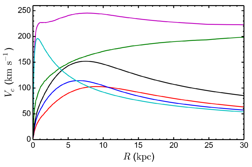
Figure 1: Circular speed curve decomposition for our Milky Way-like model. The solid magenta curve shows the total circular speed of the model. Also shown are the contributions to the circular speed curve from the bulge (cyan), halo (green), thin disc (blue), thick disc (red), and total disc (black).

Our choice of disc parameters is guided by the analysis of Bovy et al. (2012) and Bovy & Rix (2013) as well as our desire for a model that is stable against the formation of a bar for the duration of the simulation runtime. As discussed in Section 1, this model allows us to focus on the effect substructure, rather than a bar or large-amplitude spiral structure, has on vertical oscillations. The thin disc has a radial exponential scale length of $3.6\mskip 3.0mu{\rm kpc}$ and a mass of $2.6\times 10^{10}\mskip 3.0muM_{\odot}$. The corresponding quantities for the thick disc are $2.0\mskip 3.0mu{\rm kpc}$ and $2.2\times 10^{10}\mskip 3.0muM_{\odot}$. The total disc mass of $4.8\times 10^{10}\mskip 3.0muM_{\odot}$ is in accord with the total stellar disc mass for the Milky Way reported in the literature (Bovy & Rix 2013, but see also Courteau et al. 2014 for a review). The vertical structure of the discs are well-described by a ${\rm sech}^{2}(z/2\mskip 3.0muz_{d})$ profile with $z_{d}$ = $260\mskip 3.0mu{\rm pc}$ for the thin disc and $690\mskip 3.0mu{\rm pc}$ for the thick (Bovy et al., 2012).

Our bulge has a target density profile given by the Hernquist profile (equation 1 with $\left(\alpha,\mskip 3.0mu\beta\right)=\left(1,\mskip 3.0mu4\right)$) and a total mass of $2\times 10^{10}~{}M_{\odot}$, which is slightly higher (by about 5-10 per cent) than the current best estimates for the Milky Way’s bulge (see Bland-Hawthorn & Gerhard, 2016). The bulge scale radius is taken to be $600\mskip 3.0mu{\rm pc}$ as in the Bovy & Rix (2013) model and the velocity distribution is approximately isotropic.

The halo target density profile is given by the NFW profile (equation 1 with $\left(\alpha,\mskip 3.0mu\beta\right)=\left(1,\mskip 3.0mu3\right)$; see Navarro et al. 1996) with scale radius $r_{b}=22\mskip 3.0mu{\rm kpc}$ and $\rho_{0}=9\times 10^{6}M_{\odot}\mskip 3.0mu{\rm kpc}^{-3}$. The parameters for the DF are chosen so as to yield a total circular speed curve that is approximately flat with $V_{c}\simeq 220-250\mskip 3.0mu{\rm km\mskip 3.0mus^{-1}}$ for $2\mskip 3.0mu{\rm kpc}<R<30\mskip 3.0mu{\rm kpc}$ (see Fig. 1). Note as well that the total disc is submaximal. In particular, $V_{d}^{2}/V_{c}^{2}\approx 0.37$ at the peak of the total disc’s circular speed curve ($R\sim$7 kpc), where $V_{d}$ is the contribution to the circular speed from the total disc.

Fig. 2 shows the surface density profiles of the thin and thick discs. We note that, at small radii, the surface densities are supressed relative to a pure exponential. This effect is likely due to the presence of a cuspy bulge and the fact that in action-based modelling the resulting density law is only approximately equal to the target. Our Hernquist bulge causes the epicyclic frequencies to rapidly increase as $R\to 0$ and consequently the pseudo-isothermal DF is not well behaved in the central disc (Vasiliev, 2018).

The root-mean-square thicknesses of the discs in our model vary with $R$ by a factor of $\sim 2$ as seen in the middle panel of Fig. 2. The depression at small radii is, again, due to the inclusion of a cuspy bulge. The decrease in thickness at larger radii is presumably due to using an exponential vertical velocity dispersion profile, which would produce a constant scale height only for a thin disc in isolation.

The central radial dispersion was chosen to yield a relatively high Toomre $Q$ parameter (Toomre, 1964) across the disc, as can been seen in the bottom panel of Fig. 2. The fact that we have a submaximal disc with $Q>1.5$ indicates that very little structure will develop in the disc, at least in the absence of external perturbations.

In the top panel of Fig. 3 we show the vertical density profiles for the thin, thick, and total discs evaluated at $R=8\mskip 3.0mu{\rm kpc}$. On average, the density profiles roughly correspond to our target parameters. In the bottom panel we show the vertical velocity dispersion profile, and see that the thin and thick discs are roughly isothermal. The vertical profiles are shown for the Solar circle though the same general trends are observed at all other radii.

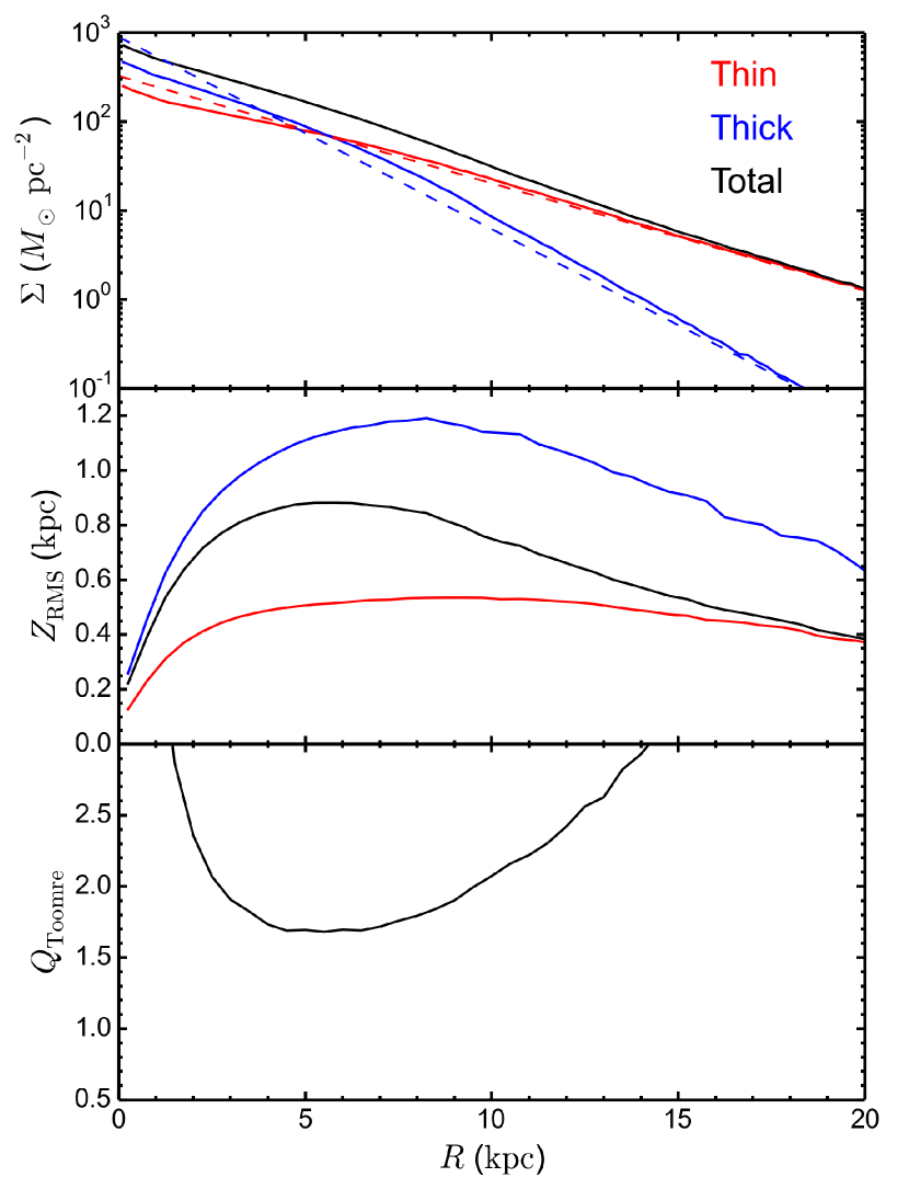
Figure 2: Radial properties of our Milky Way-like disc. The colour corresponds to the thin (red), thick (blue), and total (black) discs. Top panel: Surface density profiles. Solid lines correspond to our $N$-body model and dashed lines indicate the target profiles. Middle panel: Root-mean-square height profiles. Bottom panel: Toomre $Q$ parameter profile of the total disc.

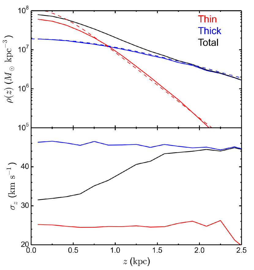
Figure 3: Vertical properties of our Milky Way-like disc evaluated at a galactocentric radius of 8 kpc. The colour corresponds to the thin (red), thick (blue), and total (black) discs. Top panel: Vertical density profiles. Solid lines correspond to our $N$-body model and dashed lines indicate the target profiles. Bottom panel: Vertical velocity dispersion as a function of distance from the midplane.

2.2 Halo substructure

For our satellite simulation we replace 10 per cent of the halo mass with 100 subhaloes by a scheme similar to the one presented in Gauthier et al. (2006). We randomly remove 10 per cent of the particles that characterize the smooth halo and insert an equivalent amount of mass in the form of spherical subhaloes. These subhaloes have initial center-of-mass positions and velocities drawn from the same DF as the original halo.

The initial cumulative distribution of subhaloes as a function of galactocentric radius is shown in Fig. 4. Note that while only a few subhaloes begin with an initial radius inside the region of the disc (i.e., $r\la 30\mskip 3.0mu{\rm kpc}$), $20$ or so subhaloes follow orbits with a perigalacticon less than $30\mskip 3.0mu{\rm kpc}$. Thus, most of the subhaloes that pass through the disc were initialized well outside the disc region.

We assume an initial subhalo mass function given by

$${dN_{\rm sat}\over dM_{\rm sat}}~{}=~{}\left\{\begin{array}[]{@{}l@{\quad}l@{}}AM_{\rm sat}^{-2}&\text{for}~{}M_{\rm min}\leq M_{\rm sat}\leq M_{\rm max}~{},\\ 0&\text{otherwise}~{},\end{array}\right.$$ (3)

where $A$ is a normalization constant. In addition, we assume that the total mass in subhaloes is one tenth of the virial mass of the halo and the maximum subhalo mass is $M_{\rm max}=0.1\left(M_{\rm disc}+M_{\rm bulge}\right)$. These two conditions allow us to determine $M_{\rm min}$ and $A$. Equation (3) is then sampled to determine initial virial masses for the subhaloes. We use galactics (Kuijken & Dubinski, 1995; Widrow et al., 2008) to generate $N$-body realizations of the subhaloes assuming that each has a truncated NFW density profile. galactics requires the specification of NFW mass in addition to scale and truncation radii. We compute scale radii for each subhalo as $c=r_{200}/a_{s}$, where $c$ is the halo concentration, $r_{200}$ is the radius in which the mean halo density is 200 times the critical density, and $a_{s}$ is the NFW scale radius. We adopt a constant value of $c=20$ for all of the subhaloes, which is in agreement with cosmological simulations for the mass range of our subhalo population over a significant look-back time ($\sim$10 Gyr) (Macciò et al., 2007; Zhao et al., 2009). A histogram of the subhaloes as a function of their virial mass is shown in Fig. 5.

We smoothly truncate the $N$-body subhaloes at their tidal radii which are numerically computed using the Jacobi approximation (Binney & Tremaine, 2008, section 8.3)

$$\bar{\rho}_{\rm sat}(r_{t})=3\bar{\rho}_{\rm halo}(r_{\rm sat}),$$ (4)

where $\bar{\rho}_{\rm sat}(r_{t})$ is the subhalo’s mean density inside the truncation radius $r_{t}$, and $\bar{\rho}_{\rm halo}$ is the mean density of the halo inside the initial radius, $r_{\rm sat}$, of the subhalo. Truncation is meant to take into account tidal stripping that may have occurred prior to the initial epoch of the simulation.

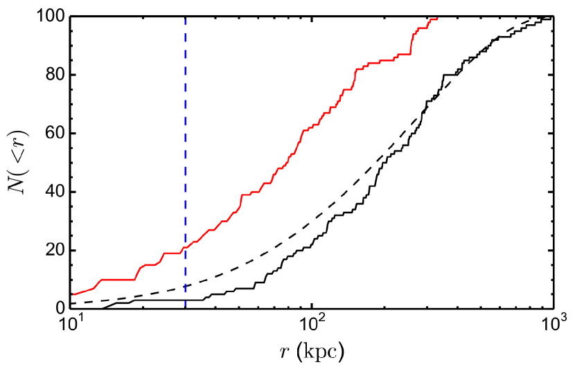
Figure 4: Cumulative number distribution of initial center-of-mass subhalo radius within the host halo (solid black). The dashed black curve is the normalized cumulative number distribution of particles in the smooth halo from which the positions of the subhalo system were sampled. The solid red line shows the cumulative distribution of initial pericentre distances of the subhalo population. The vertical dashed blue line references the initial edge of the disc.

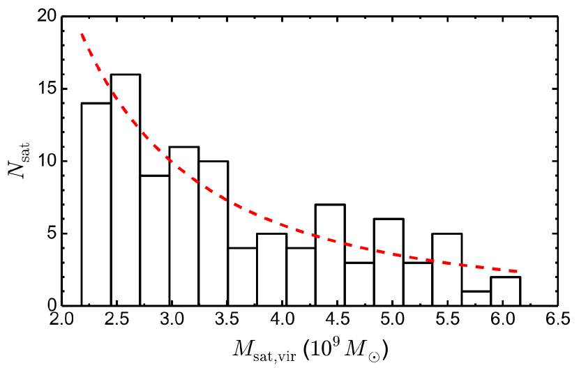
Figure 5: Number distribution of substructure virial mass. Solid black represents the distribution of the substructure population in our subhalo model. The dashed red curve corresponds to the number distribution derived from the mass spectrum from which our population was sampled (equation 3).

2.3 $N$-body simulations

Multidimensional sampling routines built into agama were used to generate an $N$-body realization of our model galaxy with $2.5M$ thin disc, $2.5M$ thick disc, $250k$ bulge, and $5M$ halo particles. When subhaloes were included, the smooth component of the halo had $4.5M$ particles while each subhalo had $25k$ particles. The initial conditions were evolved for $\sim 10\mskip 3.0mu{\rm Gyr}$ using gadget-3 (Springel, 2005) with softening lengths of $40$, $15$, $100$, and $80$ pc for the disc, bulge, halo, and subhalo particles, respectively. The maximum time step was set to $0.18\mskip 3.0mu{\rm Myr}$, which is $\sim$0.6 per cent of the galactic dynamical time defined at the radius of peak disc contribution to the rotation curve, $R\sim 7$ kpc. Total energy was conserved to within 0.06 per cent. The ratio of total kinetic to potential energy for the particle distributions comprising the thin and thick discs, bulge, and halo in the isolated model was $-0.503$, $-0.502$, $-0.505$, and $-0.503$, respectively, indicating that the initial conditions were sufficiently close to equilibrium. Indeed, in the first 250 Myr we observed a maximum increase in the vertical velocity dispersion and $Z_{RMS}$ profiles of only $\sim 1\mskip 3.0mu{\rm km}\mskip 3.0mu{\rm s}^{-1}$ and $\sim 60\mskip 3.0mu{\rm pc}$, respectively.

Over time the discs in our simulations rotate and drift about the global coordinate origin, particularly in the simulation with halo substructure. To account for this when analyzing our models we center and rotate all model components by the following scheme: We first iteratively compute the center of mass of disc particles within a cylinder of radius $20\mskip 3.0mu{\rm kpc}$ and height $2\mskip 3.0mu{\rm kpc}$. Next, we reorient the system so that the disc lies in the $x$-$y$ plane by using a two-dimensional Newton-Raphson scheme to find the orientation that minimizes the root mean square vertical displacement of disc particles within the same cylinder used to find the centre of mass.

3 Disc-Subhalo interactions

In this section we focus on the evolution of the subhalo population in our satellite simulation. We define the position and velocity of a particular subhalo as the average position and velocity of its 100 initially most energetically bound particles. This method does a good job at accurately tracking the phase space coordinates of a subhalo until it is completely disrupted. Computation of the bound mass within each subhalo has historically involved an iterative procedure concerning energy calculations (e.g. Benson et al., 2004). Here, we employ a simpler approach where the bound mass of each subhalo at each time output is taken to be the mass contained within the Jacobi sphere as defined in equation (4).

In Fig. 6 we show the temporal evolution of the mass bound in subhaloes relative to the total mass of the halo and subhalo population. Our initial total substructure mass fraction, $\sim 0.08$, is in rough agreement with that of Milky Way-like haloes found in cosmological simulations, such as the Aquarius Project (Springel et al., 2008, figure 12). If we consider only subhaloes initiated within a radius of 50 kpc, the substructure mass fraction decreases to $\sim 10^{-2}$. This value also agrees with that found by the Aquarius Project, although in the case of our simulation is due to the stochastic nature of sampling the initial positions and masses of only 100 subhaloes. This is supported by Fig.  4, where the inner galaxy contains fewer subhaloes than expected, and the fact that those subhaloes initiated within a radius of $\sim$ 90 kpc have masses from the lower end of the mass spectrum we sampled.

Our results can also be compared with those from Gauthier et al. (2006) who argued that the time-dependence of the mass in subhaloes could be described by two distinct phases. During the first $4\mskip 3.0mu{\rm Gyr}$ $f\propto\exp{\left(-t/\tau_{f}\right)}$ with $\tau_{f}\simeq 5.1\mskip 3.0mu{\rm Gyr}$, while from $4$ to $10\mskip 3.0mu{\rm Gyr}$ $\tau_{f}\simeq 13.4\mskip 3.0mu{\rm Gyr}$. We find a similar trend where the exponential decay rate of subhalo mass descreases with time, though our initial ‘rapid decay phase’ is shorter. The difference may be a simple reflection of the fact that our distribution extends to much larger radii and therefore a greater fraction of our subhaloes do not experience tidal disruption.

The amplitude and extent of a perturbation in the disc due to a passing subhalo will depend on the position at which the subhalo’s orbit crosses the disc plane, its mass and velocity, and the orientation of the orbital angular momentum vector with respect to that of the disc’s (i.e. prograde, retrograde, or vertical orbits; Gómez et al., 2013; Widrow et al., 2014; Feldmann & Spolyar, 2015). The two panels in Fig. 7 are meant to give a sense of which subhaloes will cause the most significant perturbations. In both panels we show the times and cylindrical radii at which a subhalo crosses the disc midplane. In the top panel we colour the points according to the ratio of subhalo surface density to the locally azimuthally averaged surface density of the disc at the time of impact. The restoring force of the disc is proportional to the disc surface density, so by comparing this with the corresponding quantity for the subhaloes we get a sense of how significantly a given interaction might perturb the vertical structure of the disc. In general, we see that the subhaloes that cross the disc plane with $R<10\mskip 3.0mu{\rm kpc}$ have relatively low surface densities, except perhaps during the first few ${\rm Gyr}$. The number of significant subhalo interactions (interactions where the subhalo surface density is comparable to or greater than that of the disc) increases significantly at larger radii, in part because the density of the disc decreases exponentially, and in part because subhaloes tend to be disrupted if their orbits take them close to the galactic centre.

In the bottom panel of Fig. 7 we show the subhalo’s vertical velocity as it passes through the disc midplane relative to the local vertical velocity dispersion of the disc as a function of $R$ and simulation time. We see that satellites that pass through the outer disc have speeds 10-100 times higher than the typical vertical velocities of the disc stars. In this region, the epicyclic motion can all but be ignored during a subhalo-disc interaction. Conversely, subhaloes passing through the disc at intermediate radii ($5\mskip 3.0mu{\rm kpc}<R<15\mskip 3.0mu{\rm kpc}$) have vertical velocities more typical of the vertical velocities in the disc. This sets up the possibility for resonant excitation of both vertical bending and breathing waves (Sellwood et al., 1998; Widrow et al., 2014).

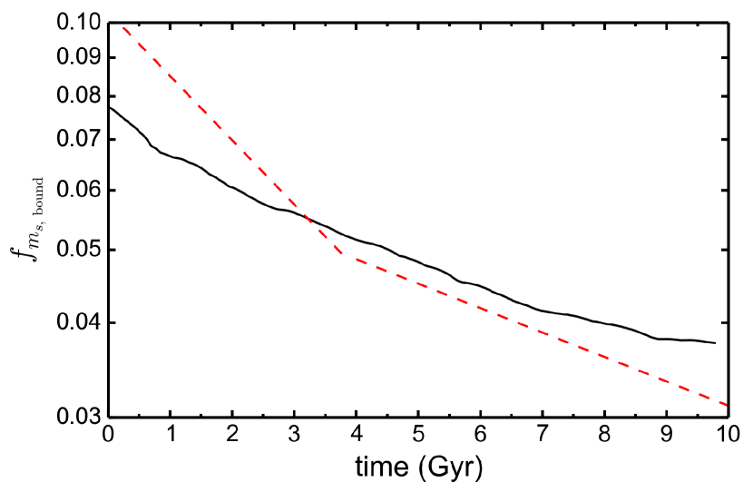
Figure 6: Mass bound to subhaloes relative to the total mass contained in the halo and subhalo population as a function of time (solid black). For comparison we also show the corresponding relation for the two distinct phases of subhalo mass loss in the Gauthier et al. (2006) simulation (dashed red).

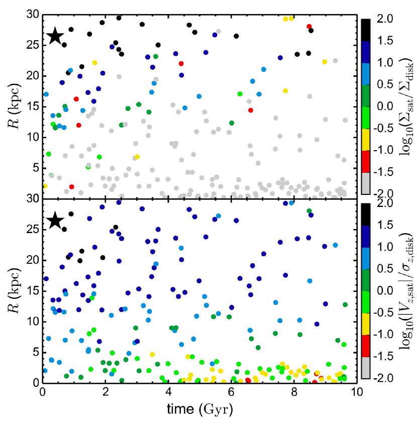
Figure 7: Time evolution of subhalo impacts on the disc. Each point represents the cylindrical radius and the time at which a subhalo crosses the $z=0$ plane. The star symbol indicates the specific impact event discussed in Section 4. Colour coding in the top panel corresponds to the ratio of projected subhalo surface density to that of the local disc at the time of impact - a proxy for the efficacy of each impact to produce vertical waves. In the bottom panel, the colour corresponds to the ratio of subhalo vertical velocity to the local vertical velocity dispersion of the disc at that time.

4 Fourier analysis of density and vertical waves

In Fig. 8 we show the normalized surface density in the disc, $\Sigma\left(R,\mskip 3.0mu\phi,\mskip 3.0mut\right)/\Sigma\left(R,\mskip 3.0mut_{0}\right)$, where $\Sigma\left(R,\mskip 3.0mut_{0}\right)$ is the initial surface density profile (see top panel Fig. 2). The normalization is chosen to highlight non-axisymmetric features that develop across the full range in $R$. Evidently, neither disc forms a bar. The disc in the control simulation develops tightly wrapped flocculent spiral arms with a density contrast that tends to be more pronounced at late times and toward the outer region of the disc. The spiral structure is considerably stronger in the satellite simulation. At early times the density features are more asymmetric and irregular. Note, in particular, what appears to be evidence of a single satellite interaction in the $t=500\mskip 3.0mu{\rm Myr}$ snapshot at $R\sim 20-25\mskip 3.0mu{\rm kpc}$ and roughly the ‘5-o’clock’ position of the disc. At later times large density contrasts survive only past $R\sim 10-15\mskip 3.0mu{\rm kpc}$ and extend in azimuthal angle around a large fraction of the disc. By the end of the simulation the disc develops a dominant $m=1$ spiral arm that is morphologically leading. We attribute these density enhancements and morphological differences to collisions or torques imparted from the orbiting subhalo system since they are not present in the control run (Gauthier et al., 2006; Dubinski et al., 2008).

In Fig. 9 we show vertical displacement, $Z\left(R,\mskip 3.0mu\phi,\mskip 3.0mut\right)$, across the disc at the same epochs as those shown in Fig. 8. The trends are similar to those seen in the surface density plot. Bending waves appear in both the control and satellite simulations though they have a higher amplitude by a factor of $\sim 5$ in the satellite case. In both cases, strength in the bending waves tends to migrate toward the edge of the disc over time.

At early times, there are localized bending waves in the satellite case. In particular, we see evidence of an apparent interaction event in the $500\mskip 3.0mu{\rm Myr}$ snapshot at the same location in the disc as seen in the surface density, and have identified the subhalo responsible for this event. This satellite plunged through the disc midplane at a radius of $\sim$ 26.5 kpc at $\sim$ 400 Myr (indicated by the star symbol in Fig. 7) on a prograde orbit with cylindrical velocities $(V_{R},V_{\phi},V_{z})\simeq(-160,\mskip 3.0mu50,\mskip 3.0mu210)\mskip 3.0mu{\rm km}\mskip 3.0mu{\rm s}^{-1}$. At the time of impact the satellite had a mass of $\sim 8\times 10^{8}\mskip 3.0muM_{\odot}$ within its 2.7 kpc radius Jacobi sphere. Despite crossing through the disc with such a large vertical velocity, the radial extent, surface density, and in-plane velocity of the satellite are significant, and therefore it is not surprising that the impact left such a clear and spatially extended mark in the disc, as seen in Figs. 8 and 9.

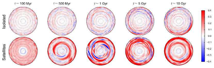
Figure 8: Surface overdensity for the control (top row) and satellite (bottom row) simulations at five epochs. The colour map indicates the logarithm (base 10) of the ratio of the local surface density at the time indicated to the azimuthally-average surface density of the initial conditions. Dotted concentric circles indicate increments of 5 kpc in radius. The rotation of the discs is counter-clockwise.

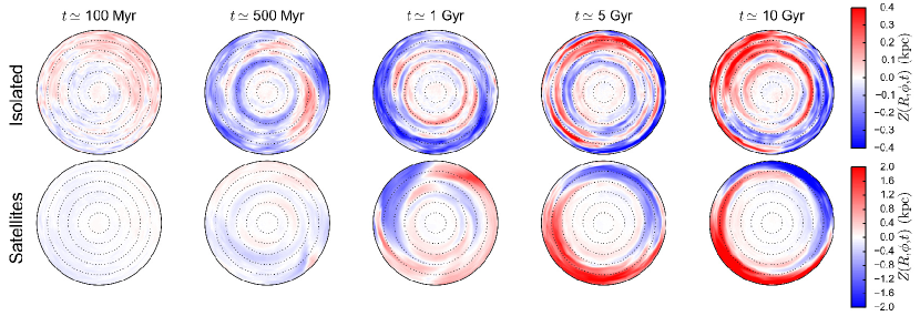
Figure 9: Face-on maps of mean vertical displacement $Z(R,\phi,t)$ for the isolated (top row) and satellite (bottom row) simulations at the same five epochs in Fig. 8. Dotted concentric circles indicate increments of 5 kpc in radius. The rotation of the discs is counter-clockwise.

We next consider the application of Fourier methods to the simulations. Formally, the DF of an $N$-body system can be expressed as the sum of six-dimensional $\delta$-functions centred on the phase space coordinates (positions and velocities) of the particles and weighted by their mass. The density is found by integrating over velocities while the surface density is found by further integrating over $z$. Thus, the surface density is given by

$$\Sigma\left(R,\mskip 3.0mu\phi,\mskip 3.0mut\right)=\sum_{j}m_{j}\mskip 3.0mu\delta\left(\phi-\phi_{j}(t)\right){\delta\left(R-R_{j}(t)\right)\over R}~{}.$$ (5)

(For the maps in Fig. 8 we effectively integrate over bins in a polar grid and divide by the area of each bin. In Fig. 9, we compute the average $z$ in each of these bins).

Beginning with the pioneering work of Sellwood & Athanassoula (1986) it has proved useful to consider various transforms of the surface density when studying the formation of warps, bars, and spiral structure. A Fourier series in $\phi$ yields a decomposition of $\Sigma$ in terms of azimuthal wave number $m$, with warps dominated by $m=1$ while bars and bisymmetric spiral structure are dominated by $m=2$. A Fourier transform in $t$ yields the surface density amplitude as a function of $\omega$, $R$, and $\phi$, or $\omega$, $R$, and $m$. The frequency $\omega$ can be used as a proxy for angular pattern speed. Sellwood & Athanassoula (1986) also consider a Fourier transform in $\ln{R}$.

In what follows, we apply Fourier methods to bending waves. We begin by dividing the disc into cencentric rings each labelled by $\alpha$ and centred on a radius $R_{\alpha}$ with width $\Delta R_{\alpha}$ and surface area $S_{\alpha}\equiv 2\pi R_{\alpha}\Delta R_{\alpha}$. The radially-smoothed surface density is then

$$\Sigma\left(R_{\alpha},\mskip 3.0mu\phi,\mskip 3.0mut\right)=2\pi\mskip 3.0muS_{\alpha}^{-1}\sum_{j\in\alpha}m_{j}\mskip 3.0mu\delta\left(\phi-\phi_{j}(t)\right)~{},$$ (6)

where $R_{\alpha}\rightarrow R$ in the limit of small $\Delta R_{\alpha}$ and the sum is over all particles in ring $\alpha$. The vertical displacement, $Z\left(R,\mskip 3.0mu\phi,\mskip 3.0mut\right)$, and vertical bulk motion, $V_{z}\left(R,\mskip 3.0mu\phi,\mskip 3.0mut\right)$, can be constructed by taking moments of the DF. In analogy with equation (6) we have

$$Q\left(R_{\alpha}\mskip 3.0mu\phi,\mskip 3.0mut\right)=2\pi\mskip 3.0muS_{\alpha}^{-1}\mskip 3.0mu\Sigma^{-1}\left(R_{\alpha},\mskip 3.0mu\phi,\mskip 3.0mut\right)\sum_{j\in\alpha}m_{j}\mskip 3.0muq_{j}(t)\mskip 3.0mu\delta\left(\phi-\phi_{j}(t)\right)~{},$$ (7)

where $Q=\left\{Z,\mskip 3.0muV_{z},\mskip 3.0mu\mathellipsis\mskip 3.0mu\right\}$ and $q_{j}=\left\{z_{j},\mskip 3.0muv_{z,j},\mskip 3.0mu\mathellipsis\mskip 3.0mu\right\}$, and the $\mathellipsis\mskip 3.0mu$ refer to any non-linear function of $z$ and $v_{z}$.

The Fourier series for the surface density is given by

$$\Sigma\left(R_{\alpha},\mskip 3.0mu\phi,\mskip 3.0mut\right)=\sum_{m=0}^{\infty}\Sigma_{m}(R_{\alpha},\mskip 3.0mut)e^{-im\phi}~{},$$ (8)

where

(9)

Likewise, the Fourier coefficients of $Q\left(R_{\alpha},\mskip 3.0mu\phi,\mskip 3.0mut\right)$ are

$$Q_{m}(R_{\alpha},\mskip 3.0mut)=S_{\alpha}^{-1}\sum_{j\in\alpha}{m_{j}\mskip 3.0muq_{j}\mskip 3.0mue^{-im\phi_{j}}\over\Sigma\left(R_{j},\mskip 3.0mu\phi_{j},\mskip 3.0mut\right)}~{},$$ (10)

where $\Sigma\left(R_{j},\mskip 3.0mu\phi_{j},\mskip 3.0mut\right)$ is the interpolated surface density at the position of the $j$th particle.

In Fig. 10 we plot $|\Sigma_{1}(R,\mskip 3.0mut)|\mskip 3.0mu/\mskip 3.0mu\Sigma(R,\mskip 3.0mut_{0})$, $|Z_{1}(R,\mskip 3.0mut)|$, and $|V_{z,1}(R,\mskip 3.0mut)|$. In particular, we show the separate contributions from the thin and thick discs, and compare the isolated and satellite simulations. Generally, we see that the thick disc is much less responsive by a factor of $4\sim 5$ and the subhaloes induce perturbations with peak amplitudes $\sim 5$ times greater than those in the control simulation.

Bending waves are strongest in the outer disc for both control and satellite runs. This result is expected for several reasons. First, the transition from a relatively quiet disc to one with stronger vertical waves occurs at $R\sim 15{\rm kpc}$, which roughly coincides with region where the surface density of the thick disc falls to negligible values. Thus, the increased gravity from a relatively warm component may make the inner disc less responsive to bending perturbations. Moreover, the higher surface density of the thin disc itself acts to stiffen the disc. The outer disc is dominated by the cooler thin disc though much of the gravitational field is from the halo, and it is therefore more prone to non-axisymmetric structure formation and bending waves. Finally, as noted in section 3 the strongest subhalo encounters occur in the outer disc.

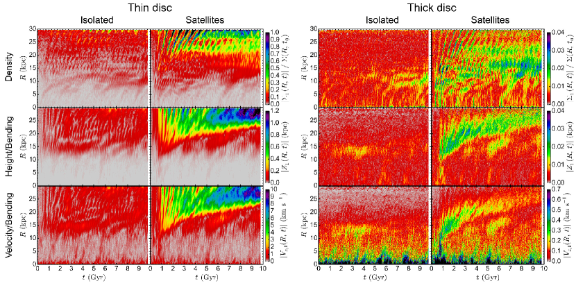
Figure 10: Time evolution of $m=1$ Fourier coefficients for in-plane density and bending waves in both the thin and thick discs of the isolated and satellite simulations, as indicated. Note the difference in colour scale between the thin and thick discs.

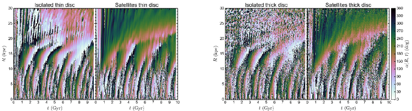
Figure 11: Time evolution of Fourier phase angle $\alpha(R,\mskip 3.0mut)$ for $m=1$ vertical displacement bending waves in the thin and thick discs of both simulations, as indicated.

To determine the morphology of $m=1$ bending waves we compute the complex phase for $Z_{1}$,

$$\alpha(R,\mskip 3.0mut)={\rm tan}^{-1}{\hbox{\frozen@everymath=0pt$\left[\vbox to0.0pt{}\right.$}}{{\rm Im}\{Z_{1}(R,\mskip 3.0mut)\}\over{\rm Re}\{Z_{1}(R,\mskip 3.0mut)\}}{\hbox{\frozen@everymath=0pt$\left]\vbox to0.0pt{}\right.$}}~{},$$ (11)

as a function of $R$ and $t$. In Fig. 11 we show $\alpha(R,\mskip 3.0mut)$ for the thin and thick discs in both simulations. Attention is immediately drawn to ridges of constant phase that arc outward in radius over time. Since the coordinate system in our simulations has the disc rotating counter-clockwise (i.e., in the direction of increasing $\alpha$), we conclude that the bending waves are either prograde and trailing or retrograde and leading. A distinction between the two cases is made when considering the behaviour of $\alpha$ over slices in $R$ and time. The signature of leading waves is for $\alpha$ to increase with increasing $R$ at fixed time. On the other hand, the signature for a retrograde bending wave is for $\alpha$ to decrease with time at fixed $R$. Indeed, we observe these very relationships in Fig. 11 and conclude that the dominant long-lived bending waves in our simulations are morphologically leading with patterns that rotate in a retrograde sense, as is expected for bending waves (see section 8.1 of Sellwood 2013). We note that though we only show $\alpha$ for vertical displacements the phase angle for bulk vertical motions displays the same behaviour as a function of $R$ and $t$, albeit with an offset.

5 Spectral wave Analysis

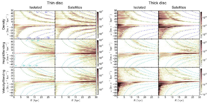
Figure 12: Frequency power spectra for $m=1$ in-plane density and bending waves in the thin and thick discs of both simulations over a time baseline of $0\leq t\lesssim 10\mskip 3.0mu{\rm Gyr}$. The layout of the figure is analogous to Fig. 10. The horizontal dashed red line references zero frequency while the dashed green curve corresponds to corotation. Overlaid as dashed blue and cyan curves are orbital resonances for kinematic density waves in a cold disc (see equation 15), as indicated, corresponding to the initial conditions.

The spectral methods developed by Sellwood & Athanassoula (1986) allow one to characterize density waves in terms of angular frequency and galactocentric radius. These methods provide valuable insight into disc dynamics and have been extended to the study of bending waves (see Chequers & Widrow, 2017).

Our spectral analysis for in-plane density waves and bending waves begins with the Fourier coefficients, $\Sigma_{m}(R,\mskip 3.0mut_{j})$ and $Q_{m}(R,\mskip 3.0mut_{j})$, for $N$ snapshots at times $t_{j}=j\mskip 3.0mu\Delta_{t}+t_{0}$, where $\Delta_{t}$ is the time between snapshots, $j=0\mathellipsis N-1$, and $N$ is even (see Fig. 10). We then perform a discrete Fourier transform on the time series to obtain the two-sided frequency coefficients (Press et al., 2007, Section 13.4) as

$$F_{m}(R,\mskip 3.0mu\omega_{k})=\left\{\begin{array}[]{@{}l@{\quad}l@{}}\Sigma^{-1}(R,\mskip 3.0mut_{0})\sum_{j=0}^{N-1}\Sigma_{m}(R,t_{j})\mskip 3.0muw(j)\mskip 3.0mue^{2\pi ijk/N},\\ \sum_{j=0}^{N-1}Q_{m}(R,t_{j})\mskip 3.0muw(j)\mskip 3.0mue^{2\pi ijk/N}~{}.\end{array}\right.$$ (12)

Here, $w(j)$ is a Gaussian window function with a standard deviation of $N/2^{5/2}$, which is introduced to diminish high-frequency spectral leakage. The discrete frequencies are given by

$$\omega_{k}={2\pi\over m}{k\over N\Delta_{t}}~{},$$ (13)

with $k=-N/2\mathellipsis N/2$. The frequency resolution is regulated by the length of the time baseline, $N\Delta_{t}$, while the Nyquist frequency, corresponding to $\omega_{k=\pm N/2}$, is derived from the time resolution, $\Delta_{t}$. The frequency power spectrum is then computed as

$$P_{m}(R,\mskip 3.0mu\omega_{k})={1\over W}\mskip 3.0mu|F_{m}(R,\mskip 3.0mu\omega_{k})|^{2}~{},$$ (14)

where $W=N\mskip 3.0mu\sum_{j=0}^{N-1}w(j)$ is the window function normalization.

In Fig. 12 we plot the frequency power spectra for $m=1$ density and bending waves over a time baseline of $0\leq t\lesssim 10\mskip 3.0mu{\rm\mskip 3.0muGyr}$. The general properties of relative frequency power between the isolated and satellite runs as well as the thin and thick discs is analogous to that of the time series of Fourier coefficient magnitude in Fig. 10 (Note the different scales used for power between the thin and thick discs).

Evidently, bending wave power follows one of a series of branches that arc across the $R$-$\omega$ plane and is concentrated in the outer disc at lower, or even counter-rotating, frequencies. These observations are in accord with our analysis in Section 4 where we concluded that the dominant waves in the disc were morphologically leading and propagate in a retrograde fashion compared to the rotation of the disc.

The power spectrum branches in Fig. 12 roughly coincide with the orbital resonance curves

$$\omega\mskip 3.0mu(R)=\left\{\begin{array}[]{@{}l@{\quad}l@{}}\Omega\mskip 3.0mu(R)+n\mskip 3.0mu\kappa\mskip 3.0mu(R),&\text{$m=1$ in-plane density waves},\\ \Omega\mskip 3.0mu(R)+n\mskip 3.0mu\nu\mskip 3.0mu(R),&\text{$m=1$ bending waves}~{}.\end{array}\right.$$ (15)

Here, $\Omega$ is the circular frequency, $\kappa$ is the total epicyclic frequency, and $\nu$ is the total vertical forcing frequency from the disc, bulge, and halo. The integer $n$ corresponds to the number of azimuthal periods an orbit takes to close during one radial oscillation period in a frame rotating with angular frequency $\omega$. The Lindblad resonances and their vertical analogs correspond to $n=\pm 1$.

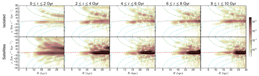
Figure 13: Time evolution of $m=1$ height/bending frequency power spectra evaluated over $\sim$ 2 Gyr intervals for the thin disc in both simulations, as indicated. The dashed curves correspond to the same quantities as in Fig. 12.

Many of the features in Fig. 12 can be understood by appealing to the WKB approximation, where one assumes that the waves (either density or bending) are tightly wound. In this approximation, and under the further assumption that the disc is cold and thin, the dispersion relations are (Binney & Tremaine, 2008, sections 6.2.1 and 6.6.1, and section 8.1 from Sellwood 2013)

$$(\omega-\Omega)^{2}=\left\{\begin{array}[]{@{}l@{\quad}l@{}}\kappa^{2}-4\pi^{2}G\Sigma/\lambda_{\rm d},&\text{for $m=1$ density waves},\\ \nu^{2}+4\pi^{2}G\Sigma/\lambda_{\rm b},&\text{for $m=1$ bending waves,}\end{array}\right.$$ (16)

where $\Sigma$ is the radial surface density and $\lambda_{\rm d}$ $(\lambda_{\rm b})$ is the wavelength of a density (bending) wave. From equation (16) we see that WKB density waves are ‘forbidden’ in the region outside the Lindblad resonances while bending waves are forbidden between the corresponding vertical resonances (equation 15). Indeed, we find that in the case of density waves power mainly lies between the Lindblad resonance curves whereas power lies outside the $n=\pm 1$ vertical resonances in the case of bending waves.

The Lindblad resonances and their vertical analogs emerge from equation (16) in the limit that the surface density terms (i.e. the terms that encode the forcing frequency due to the self-gravity of the perturbation) on the right hand side are negligible when compared to the $\kappa^{2}$ or $\nu^{2}$ terms. Thus, we can predict the degree to which power should align with the resonance curves by comparing the two terms on the right-hand side of equation (16). In general, we expect this alignment to be better at large radii since the surface density falls off exponentially while $\kappa$ and $\nu$ fall as as powers of $R$. Furthermore, following similar arguments to those found in Binney & Tremaine (2008, equation 3.89), one can show that

$${\nu^{2}\over\kappa^{2}}\simeq{3\over 2}{\rho\over\bar{\rho}}$$ (17)

where $\bar{\rho}$ is the mean density within a given radius and $\rho$ is the density of the galaxy in the midplane of the disc at that radius. Since the bulge and halo are nearly spherically symmetric with monotonically decreasing density profiles and the submaximal disc lies in the plane, we conclude that $\nu<\kappa$. Therefore the surface density term in equation (16) will play a larger role for bending waves than for density waves. It is therefore not surprising that bands in power are more closely aligned with the resonance curves in the density wave case than the bending wave one.

In Fig. 13 we show a time sequence of $m=1$ bending waves over $\sim$ 2 Gyr intervals for the thin disc. For each of the time intervals in the control simulation, power lies along branches just outside the $n=\pm 1$ resonance curves, as expected. The situation is more complicated in the case with satellites. At early times, there are numerous regions of power across the $R-\omega$ plane that are not particularly well correlated with the resonance curves. Over time, the positive frequencies diminish in power, although localized waves still exist, and the strength of low-frequency counter-rotating waves increases in strength and migrates outward. By the end of the simulation, the branches of power roughly mirror that of the isolated simulation, though the relative weighting of the waves localized in radius is quite different. These results make intuitive sense. Bending waves in the control simulation involve the growth of linear perturbations, which are well described by a WKB analysis. The satellite-provoked waves, on the other hand, are more random in nature, though over time, the most persistent ones also appear to coincide with predictions from linear theory.

6 Correlation between $Z$ and $V_{z}$

Simultaneous observations of bulk vertical motions and vertical displacement provide an avenue toward understanding wave dynamics in the Galactic disc. Roughly speaking the angular frequency of a wave will be given by the amplitude of its oscillations in velocity divided by the amplitude of its displacement oscillations. Xu et al. (2015) found evidence for corrugations in the disc with an amplitude of about $120\mskip 3.0mu{\rm pc}$ and a wavelength of $7\mskip 3.0mu{\rm kpc}$ at Galactocentric radii of $10-16\mskip 3.0mu{\rm kpc}$. On the other hand, Schönrich & Dehnen (2017) identified ripples in the velocity field of the Solar Neighbourhood with an amplitude of $\sim 0.8\mskip 3.0mu{\rm km\mskip 3.0mus^{-1}}$ and a wavelength of $2-2.5\mskip 3.0mu{\rm kpc}$. Of course, the wavelength and amplitude of a bending wave might change with Galactocentric radius. As noted in Schönrich & Dehnen (2017), the extent of their sample was not sufficient to detect such changes. In any case, if one assumes that the Xu et al. (2015) and Schönrich & Dehnen (2017) oscillations are related, then the inferred angular frequency is $\simeq 6.7\mskip 3.0mu{\rm km\mskip 3.0mus}^{-1}{\rm kpc}^{-1}$, which correponds to a period of about $920\mskip 3.0mu{\rm Myr}$. Obviously, the caveats mentioned above imply that this is only a ballpark value and valid only if the two observations are of the same wave-like structure.

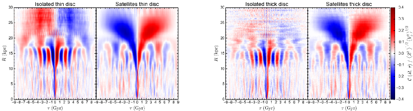
Figure 14: Normalized cross correlation (see equations 18 and 19) between $m=1$ velocity and displacement bending waves. The column titles indicate which disc and simulation each panel corresponds to.

The correlation between bulk vertical motion and midplane displacement in simulations has been discussed by Gómez et al. (2013), Gómez et al. (2016), Chequers & Widrow (2017), and Gómez et al. (2017). In both of our control and satellite simulations the bulk vertical motions follow the same general patterns as the displacements (c.f. Figs. 10-12) except for a phase offset. This behaviour is expected for wave-like motion and allows one to infer a rotational frequency from the respective amplitudes of each pattern.

To further explore the connection between velocity and displacement oscillations, we compute the azimuthally-averaged cross correlation function between $Z_{1}$ and $V_{z,1}$:

$$\mathcal{C}\mskip 3.0mu(R,\mskip 3.0mu\tau)={1\over 2\pi}\intop\nolimits_{0}^{2\pi}d\phi\mskip 3.0mu{1\over t_{f}}\intop\nolimits_{0}^{t_{f}}V_{z,1}(R,\mskip 3.0mu\phi,\mskip 3.0mut)\mskip 3.0muZ_{1}(R,\mskip 3.0mu\phi,\mskip 3.0mut+\tau)\mskip 3.0mudt~{},$$ (18)

where $\tau$ is the lag time between the signals. To highlight small amplitude wave-like features we normalize to the root-mean-square of $Z$ and $V_{z}$ at a given radius,

$$\langle Q^{2}\rangle^{1/2}=\sqrt{{1\over t_{f}}\intop\nolimits_{0}^{t_{f}}q^{2}(t)\mskip 3.0mudt}~{},$$ (19)

where $Q=\{Z,\mskip 3.0muV_{z}\}$ and $q=\{z,\mskip 3.0muv_{z}\}$, respectively.

For the highly idealized case of a linear one-dimensional monochromatic plane wave, the displacement, $z=D\mskip 3.0mu{\rm sin}(\omega t+\phi)$, is related to the velocity by $v=d\mskip 3.0muz/dt=D\mskip 3.0mu\omega\mskip 3.0mu{\rm cos}(\omega t+\phi)$. The displacement pattern will lag the velocity by an offset in phase of $\pi/2$ and a time $\pi/2\omega$. Thus, the cross correlation between the two waveforms, $\mathcal{C}\mskip 3.0mu(\tau)\propto{\rm sin}(\omega\mskip 3.0mu\tau)$, will display periodic peaks at $2p-1$ multiples of $\tau=\pi/2\omega$, where $p$ is an integer, that decreases in amplitude with increasing $|\tau|$.

In Fig. 14 we show the normalized cross correlation between the $m=1$ displacement and velocity patterns in our simulations and immediately notice large correlation amplitudes that are localized in $R$, periodic in $\tau$, and differ between the two simulations. We also note that the radii at which these peaks in correlation amplitude occur seem to correspond to radii that feature large frequency power as seen in the spectra in Fig. 12.

Of course, in the case of our simulations the situation is more complex than simple one-dimensional monochromatic waves since our discs comprise waves of varying frequency localized in radius. Quite remarkably, for a given $R$ the cross correlation patterns we see in Fig. 14 generally exhibit the exact behaviour that is expected for simple plane waves. In particular, we observe fluctuations in amplitude that are periodic in $\tau$ and are able to recover the localized frequency $\omega=\pi/2\tau$. More globally, we see intricate patterns of correlation amplitude that highlight the dominant long-lived waves themselves and the spatial transitions between them.

We note that in the case of the thin disc in our isolated galaxy simulation for $R\gtrsim 20$ kpc the correlation amplitude is negative and positive to the right and left of zero lag, respectively, which is interpreted as the displacement pattern leading the velocity. This behaviour may indicate non-linear dynamics or damping.

7 Discussion

There is now evidence for bending and breathing waves in the stellar disc of the Milky Way from numerous astrometric surveys including GDR2. Nevertheless, the origin of these waves remains uncertain. One attractive proposal is that they are excited by interactions between the disc and satellite galaxies or dark matter subhaloes. This proposal is a natural extension of the hypothesis that satellite-disc encounters heat and thicken the disc (Toth & Ostriker, 1992) and may also prompt the formation of a bar or spiral structure (Gauthier et al., 2006; Dubinski et al., 2008; Kazantzidis et al., 2008). In the simplest interpretation wave-like features in the disc can be associated with particular disc-satellite interactions. For example, Purcell et al. (2011) used $N$-body simulations to show that the passage of the Sagittarius dwarf galaxy through the disc may have been responsible for the Milky Way’s bar and spiral structure. Gómez et al. (2013) then showed that the same encounter could generate vertical waves similar to the ones seen in the data.

The numerical experiments by Gauthier et al. (2006) and Dubinski et al. (2008) paint a more complicated picture. They simulated a disc galaxy with a clumpy halo and found that halo substructure vigourously excited spiral density waves. Moreover, even though their equilibrium (i.e., smooth halo) model was stable to bar formation for at least 10 Gyr, subhaloes could trigger the formation of a bar – though the timing of this depended on the particulars of the subhalo distribution. The implication is that the Milky Way’s dynamical state may reflect both recent, singular encounters and the cumulative effect of many disc-satellite interactions over its lifetime.

A related question concerns the evolution of perturbations once they are excited. de la Vega et al. (2015) suggested that this evolution can be described as kinematic phase mixing and that the self-gravity of the waves can be ignored. If true, this approximation would greatly simplify the analysis of perturbations in the disc. Indeed, Antoja et al. (2018) used this idea to interpret the spiral structure they found in ${\bf v}-z$ phase space projections of the GDR2 data. Simple kinematics allowed them to ‘unwind’ these structures and hence ‘date’ the event that gave rise to them.

Of course, similar arguments, when applied to the problem of spiral structure, lead to the so-called winding problem wherein spiral arms become so tightly wound in just a few orbital periods that they would dissolve into the rest of the disc. In an attempt to resolve the winding problem it was proposed that spiral arms are density waves, which are amplified and maintained by self-gravity (Lin & Shu, 1964, but see also Lindblad 1963, Lin & Shu 1966, Lin et al. 1969, and Toomre 1969). Similar arguments have been made in the study of galactic warps. For example, the eigenmode analyses of bending waves by Hunter & Toomre (1969), Sparke (1984), and Sparke & Casertano (1988) explicitly include self-gravity by treating the disc as a system of gravitationally-coupled concentric rings. When one ring is displaced from its equilibrium position, it exerts a perturbing force on the unperturbed rings and also feels a restoring force due to them. It is the combination of these two effects that yields a continuum of bending waves, which could describe the waves seen by Xu et al. (2015) and Schönrich & Dehnen (2017).

The simulations described in this paper allow us to explore these issues in more detail. In particular, we compare the evolution of a stellar-dynamical disc embedded in a clumpy dark halo with one that evolves in a smooth halo. In analyzing our simulations we turn to the spectral techniques laid out in Sellwood & Athanassoula (1986), and extended to bending waves by Chequers & Widrow (2017) (c.f. Fig. 12). We find that the dominant long-lived waves for both in-plane and vertical disturbances with $m=1$ symmetries lie mainly on or around two main branches in the $R$-$\omega$ plane, which roughly coincide with the Lindblad resonances and their vertical counterparts, and is in agreement with predictions from a linear eigenmode analysis of bending waves (Hunter & Toomre, 1969; Sparke, 1984; Sparke & Casertano, 1988, but see Chequers & Widrow 2017). However, here we make a distinction between ‘modes’ of the disc and waves since the radial locations of the waves we observe in our simulations change over time (c.f Figs 8-11) and only some of the waves appear to have somewhat well-defined frequencies. Chequers & Widrow (2017) showed that bending waves on the upper frequency branch are trailing and rotate prograde to that of the disc while the lower branch corresponds to retrograde leading waves.

Rather astonishingly, we find the dominant waves to lie on these two branches for both the isolated and satellite simulations. Therefore, the long-lived waves that the subhalo collisions excite are not haphazard, but are the very same ones that arise in the absence of halo substructure. This implies that the location of waves on the $R$-$\omega$ plane is largely dictated by the structure of the disc, which is model dependent. The $m=1$ waves we observe in face-on maps of the galaxies (i.e. Figs. 8 and 9) manifest as a superposition of waves from the two frequency branches. Any differences in bending wave morphology between the galaxies is attributed to the relative weighting of the upper and lower branches.

8 Conclusions

In this paper, we explore the continual generation of bending waves by a system of satellites or dark matter subhaloes. (Though our focus here is on bending waves, we note that higher order waves, such as breathing waves, are also generated). In particular, we show that the long-lived bending waves that arise when the halo is clumpy are qualitatively similar to, though stronger in amplitude than, the waves that arise when the halo is smooth. Of course, the degree to which bending is excited depends on the characteristics of the subhalo distribution. Therefore, the study of vertical waves could provide insight into the properties of the Milky Way’s subhalo population.

One of the main objectives of this paper is to develop analytic tools to study wave-like perturbations of the stellar disc, including those that might be observed by Gaia (See, for example, Gaia Collaboration et al. 2018a). Indeed, soon after the release of GDR2 Antoja et al. (2018) presented evidence of intriguing spiral structures in various phase space projections of the data. In that paper, the authors work under the assumption that the vertical waves are kinematic and generated by a single disc-substructure encounter. These assumptions allow them to ‘unwind’ the structure and infer an approximate epoch for when the perturbation arose.

Our simulations suggest a more complicated scenario. Consider first a single satellite that passes through the disc. Initially, the satellite transfers momentum to the disc stars thereby imprinting a local perturbation on the disc. An example can be found in Figs. 8 and 9. The perturbation is then sheared into roughly circular arcs and begins to act as a bending wave, which can propagate through the disc. Over time, energy in the wave migrates to the edge of the disc causing a warp. Energy is also dissipated into the random motions of the disc stars thus heating and thickening the disc. Thus, the waves observed today will likely involve a superposition of kinematic waves from recent events and longer lived self-gravitating waves, which evolve on timescales much longer than kinematic phase wrapping.

Much of our analysis is based on the Fourier techniques developed by Sellwood & Athanassoula (1986) for the study of in-plane density waves, and later extended by Chequers & Widrow (2017) to the case of bending waves. The time series of bending waves in the $R-\omega$ plane (Fig. 13) supports our picture. In particular, at early times in the satellite simulation power is randomly distributed across the $R$-$\omega$ plane. These perturbations, which we interpret as a superposition of kinematic waves, quickly damp and shear. At late times, after most of the satellite interactions in the inner disc have occurred, the power is more closely aligned with the resonance curves indicating the existence of more organized bending waves.

Unsurprisingly, subhalo encounters excite bending waves to a larger degree than in the case of an isolated disc. However, the two cases display similar waves in that they tend to be tightly wound, morphologically leading, and rotate in a retrograde fashion compared to that of the disc, as is expected for bending waves (Sellwood, 2013). Generally, the bending waves are dominant in the outer disc, and in particular just outside the edge of the thick disc ($R\sim 15\mskip 3.0mu{\rm kpc}$ for our Milky Way-like model). We attribute this to the increased (radial and vertical) velocity dispersion and self-gravity in the inner disc that act to resist bending (Debattista & Sellwood, 1999).

A novel feature of our simulations is the inclusion of two dynamically distinct disc components. We find that vertical bending waves are significantly weaker in the kinematically hotter thick disc than the thin one. This observation has possible ramifications for dynamical studies of the Milky Way that assume vertical equilibrium. For example, the difference in response to compression and rarefaction (breathing wave) perturbations between the thin and thick discs could lead to systematic errors in an Oort-type analysis (e.g. Bovy & Rix, 2013) for the vertical force and local surface density (see Banik et al. 2017).

The bending waves in our simulations are realized as spatial vertical displacements as well as bulk vertical motions with a phase offset (Gómez et al., 2013, 2016; Chequers & Widrow, 2017; Gómez et al., 2017). We present a cross-correlation analysis between these two manifestations of bending and find that the waves are well described by simple plane waves, and therefore their rotational frequencies can be easily inferred from the amplitudes of spatial and velocity fluctuations as seen, for example, in Xu et al. (2015) and Schönrich & Dehnen (2017).

In summary, our simulations suggest that bending of the Milky Way’s stellar disc can be understood as a superposition of waves, which lend themselves to various analysis tools such as linear theory, the WKB approximation, and spectral methods. The challenge is then to link theory and simulations of vertical waves with observations. The promise of Gaia and future projects such as the Large Synoptic Survey Telescope is that we will be able to make this linkage and gain a better understanding of the Milky Way’s disc and the environment in which it lives.

Appendix A Model parameters

In Table 1 we present the agama model parameters used to construct the initial conditions of our Milky Way-like disc.

Table 1: The most sensitive agama input file parameters for each component’s distribution function.

Component	Parameter	Value
Thin disc	Central surface density $\Sigma_{0}$ [$M_{\odot}\mskip 3.0mu{\rm pc}^{-2}$]	326
	Exponential scale radius $R_{d}$ [kpc]	3.6
	Central radial velocity dispersion $\sigma_{R,0}$ [${\rm km}\mskip 3.0mu{\rm s}^{-1}$]	103
	Central vertical velocity dispersion $\sigma_{z,0}$ [${\rm km}\mskip 3.0mu{\rm s}^{-1}$]	90
	Radial velocity dispersion exponential scale radius $R_{\sigma_{R}}$ [kpc]	7.2
	Vertical velocity dispersion exponential scale radius $R_{\sigma_{z}}$ [kpc]	7.2
Thick disc	Central surface density $\Sigma_{0}$ [$M_{\odot}\mskip 3.0mu{\rm pc}^{-2}$]	897
	Exponential scale radius $R_{d}$ [kpc]	2.01
	Central radial velocity dispersion $\sigma_{R,0}$ [${\rm km}\mskip 3.0mu{\rm s}^{-1}$]	155
	Central vertical velocity dispersion $\sigma_{z,0}$ [${\rm km}\mskip 3.0mu{\rm s}^{-1}$]	171
	Radial velocity dispersion exponential scale radius $R_{\sigma_{R}}$ [kpc]	5.5
	Vertical velocity dispersion exponential scale radius $R_{\sigma_{z}}$ [kpc]	7
Bulge	Mass normalization $M_{0}$ [$M_{\odot}$]	8.2 $\times$ $10^{10}$
	Break action $J_{0}$ [${\rm kpc}\mskip 3.0mu{\rm km}\mskip 3.0mu{\rm s}^{-1}$]	380
	Inner power law slope $\Gamma$	1.5
	Outer power law slope B	5
	Inner radial action velocity anisotropy coefficient $h_{r}$	1.2
	Inner vertical action velocity anisotropy coefficient $h_{z}$	0.9
	Outer radial action velocity anisotropy coefficient $g_{r}$	1.25
	Outer vertical action velocity anisotropy coefficient $g_{z}$	0.9
	Suppression action $J_{\rm max}$ [${\rm kpc}\mskip 3.0mu{\rm km}\mskip 3.0mu{\rm s}^{-1}$]	2800
Halo	Mass normalization $M_{0}$ [$M_{\odot}$]	5.4 $\times$ $10^{12}$
	Break action $J_{0}$ [${\rm kpc}\mskip 3.0mu{\rm km}\mskip 3.0mu{\rm s}^{-1}$]	3.3 $\times$ $10^{4}$
	Inner power law slope $\Gamma$	1.5
	Outer power law slope B	3.3
	Inner radial action velocity anisotropy coefficient $h_{r}$	1.4
	Inner vertical action velocity anisotropy coefficient $h_{z}$	0.7
	Outer radial action velocity anisotropy coefficient $g_{r}$	1.15
	Outer vertical action velocity anisotropy coefficient $g_{z}$	0.9
	Suppression action $J_{\rm max}$ [${\rm kpc}\mskip 3.0mu{\rm km}\mskip 3.0mu{\rm s}^{-1}$]	8.2 $\times$ $10^{4}$

References

- Antoja et al. (2018) Antoja T., et al., 2018, preprint, (arXiv:1804.10196)
- Araki (1985) Araki S., 1985, PhD thesis, MASSACHUSETTS INSTITUTE OF TECHNOLOGY.
- Banik et al. (2017) Banik N., Widrow L. M., Dodelson S., 2017, MNRAS, 464, 3775
- Benson et al. (2004) Benson A. J., Lacey C. G., Frenk C. S., Baugh C. M., Cole S., 2004, MNRAS, 351, 1215
- Binney (2012) Binney J., 2012, MNRAS, 426, 1324
- Binney & McMillan (2011) Binney J., McMillan P., 2011, MNRAS, 413, 1889
- Binney & Tremaine (2008) Binney J., Tremaine S., 2008, Galactic Dynamics: Second Edition. Princeton University Press
- Bland-Hawthorn & Gerhard (2016) Bland-Hawthorn J., Gerhard O., 2016, ARA&A, 54, 529
- Bovy & Rix (2013) Bovy J., Rix H.-W., 2013, ApJ, 779, 115
- Bovy et al. (2012) Bovy J., Rix H.-W., Liu C., Hogg D. W., Beers T. C., Lee Y. S., 2012, ApJ, 753, 148
- Camm (1950) Camm G. L., 1950, MNRAS, 110, 305
- Carlin et al. (2013) Carlin J. L., et al., 2013, ApJ, 777, L5
- Carrillo et al. (2018) Carrillo I., et al., 2018, MNRAS, 475, 2679
- Chequers & Widrow (2017) Chequers M. H., Widrow L. M., 2017, MNRAS, 472, 2751
- Courteau et al. (2014) Courteau S., et al., 2014, Reviews of Modern Physics, 86, 47
- D’Onghia et al. (2016) D’Onghia E., Madau P., Vera-Ciro C., Quillen A., Hernquist L., 2016, ApJ, 823, 4
- de la Vega et al. (2015) de la Vega A., Quillen A. C., Carlin J. L., Chakrabarti S., D’Onghia E., 2015, MNRAS, 454, 933
- Debattista (2014) Debattista V. P., 2014, MNRAS, 443, L1
- Debattista & Sellwood (1999) Debattista V. P., Sellwood J. A., 1999, ApJ, 513, L107
- Djorgovski & Sosin (1989) Djorgovski S., Sosin C., 1989, ApJ, 341, L13
- Drimmel & Spergel (2001) Drimmel R., Spergel D. N., 2001, ApJ, 556, 181
- Dubinski et al. (2008) Dubinski J., Gauthier J.-R., Widrow L., Nickerson S., 2008, in Funes J. G., Corsini E. M., eds, Astronomical Society of the Pacific Conference Series Vol. 396, Formation and Evolution of Galaxy Disks. p. 321 (arXiv:0802.3997)
- Faure et al. (2014) Faure C., Siebert A., Famaey B., 2014, MNRAS, 440, 2564
- Feldmann & Spolyar (2015) Feldmann R., Spolyar D., 2015, MNRAS, 446, 1000
- Ferguson et al. (2017) Ferguson D., Gardner S., Yanny B., 2017, ApJ, 843, 141
- Freudenreich et al. (1994) Freudenreich H. T., et al., 1994, ApJ, 429, L69
- Gaia Collaboration et al. (2016) Gaia Collaboration et al., 2016, A&A, 595, A1
- Gaia Collaboration et al. (2018a) Gaia Collaboration et al., 2018a, preprint, (arXiv:1804.09380)
- Gaia Collaboration et al. (2018b) Gaia Collaboration Brown A. G. A., Vallenari A., Prusti T., de Bruijne J. H. J., Babusiaux C., Bailer-Jones C. A. L., et al. 2018b, preprint, (arXiv:1804.09365)
- Gauthier et al. (2006) Gauthier J.-R., Dubinski J., Widrow L. M., 2006, ApJ, 653, 1180
- Gómez et al. (2013) Gómez F. A., Minchev I., O’Shea B. W., Beers T. C., Bullock J. S., Purcell C. W., 2013, MNRAS, 429, 159
- Gómez et al. (2016) Gómez F. A., White S. D. M., Marinacci F., Slater C. T., Grand R. J. J., Springel V., Pakmor R., 2016, MNRAS, 456, 2779
- Gómez et al. (2017) Gómez F. A., White S. D. M., Grand R. J. J., Marinacci F., Springel V., Pakmor R., 2017, MNRAS, 465, 3446
- Hernquist (1990) Hernquist L., 1990, ApJ, 356, 359
- Hunter & Toomre (1969) Hunter C., Toomre A., 1969, ApJ, 155, 747
- Kawata et al. (2018) Kawata D., Baba J., Ciucǎ I., Cropper M., Grand R. J. J., Hunt J. A. S., Seabroke G., 2018, MNRAS,
- Kazantzidis et al. (2008) Kazantzidis S., Bullock J. S., Zentner A. R., Kravtsov A. V., Moustakas L. A., 2008, ApJ, 688, 254
- Kuijken & Dubinski (1995) Kuijken K., Dubinski J., 1995, MNRAS, 277, 1341
- Lacey & Ostriker (1985) Lacey C. G., Ostriker J. P., 1985, ApJ, 299, 633
- Laporte et al. (2017) Laporte C. F. P., Johnston K. V., Gómez F. A., Garavito-Camargo N., Besla G., 2017, preprint, (arXiv:1710.02538)
- Laporte et al. (2018) Laporte C. F. P., Gómez F. A., Besla G., Johnston K. V., Garavito-Camargo N., 2018, MNRAS, 473, 1218
- Levine et al. (2006) Levine E. S., Blitz L., Heiles C., 2006, ApJ, 643, 881
- Lin & Shu (1964) Lin C. C., Shu F. H., 1964, ApJ, 140, 646
- Lin & Shu (1966) Lin C. C., Shu F. H., 1966, Proceedings of the National Academy of Science, 55, 229
- Lin et al. (1969) Lin C. C., Yuan C., Shu F. H., 1969, ApJ, 155, 721
- Lindblad (1963) Lindblad B., 1963, Stockholms Observatoriums Annaler, 22
- López-Corredoira et al. (2002) López-Corredoira M., Cabrera-Lavers A., Garzón F., Hammersley P. L., 2002, A&A, 394, 883
- Macciò et al. (2007) Macciò A. V., Dutton A. A., van den Bosch F. C., Moore B., Potter D., Stadel J., 2007, MNRAS, 378, 55
- Mathur (1990) Mathur S. D., 1990, MNRAS, 243, 529
- Minchev et al. (2009) Minchev I., Quillen A. C., Williams M., Freeman K. C., Nordhaus J., Siebert A., Bienaymé O., 2009, MNRAS, 396, L56
- Momany et al. (2006) Momany Y., Zaggia S., Gilmore G., Piotto G., Carraro G., Bedin L. R., de Angeli F., 2006, A&A, 451, 515
- Monari et al. (2015) Monari G., Famaey B., Siebert A., 2015, MNRAS, 452, 747
- Monari et al. (2016a) Monari G., Famaey B., Siebert A., 2016a, MNRAS, 457, 2569
- Monari et al. (2016b) Monari G., Famaey B., Siebert A., Grand R. J. J., Kawata D., Boily C., 2016b, MNRAS, 461, 3835
- Monari et al. (2018) Monari G., et al., 2018, Research Notes of the American Astronomical Society, 2, 32
- Navarro et al. (1996) Navarro J. F., Frenk C. S., White S. D. M., 1996, ApJ, 462, 563
- Nelson & Tremaine (1995) Nelson R. W., Tremaine S., 1995, MNRAS, 275, 897
- Pearl et al. (2017) Pearl A. N., Newberg H. J., Carlin J. L., Smith R. F., 2017, ApJ, 847, 123
- Perryman et al. (2001) Perryman M. A. C., et al., 2001, A&A, 369, 339
- Poggio et al. (2018) Poggio E., et al., 2018, preprint, (arXiv:1805.03171)
- Posti et al. (2015) Posti L., Binney J., Nipoti C., Ciotti L., 2015, MNRAS, 447, 3060
- Press et al. (2007) Press W. H., Teukolsky S. A., Vetterling W. T., Flannery B. P., 2007, Numerical Recipes. The Art of Scientific Computing, 3rd edn. Cambridge University Press
- Purcell et al. (2011) Purcell C. W., Bullock J. S., Tollerud E. J., Rocha M., Chakrabarti S., 2011, Nature, 477, 301
- Quillen et al. (2018) Quillen A. C., et al., 2018, preprint, (arXiv:1805.10236)
- Reylé et al. (2009) Reylé C., Marshall D. J., Robin A. C., Schultheis M., 2009, A&A, 495, 819
- Sanders & Binney (2016) Sanders J. L., Binney J., 2016, MNRAS, 457, 2107
- Schönrich & Dehnen (2017) Schönrich R., Dehnen W., 2017, preprint, (arXiv:1712.06616)
- Sellwood (2013) Sellwood J. A., 2013, Dynamics of Disks and Warps. p. 923, doi:10.1007/978-94-007-5612-0_18
- Sellwood & Athanassoula (1986) Sellwood J. A., Athanassoula E., 1986, MNRAS, 221, 195
- Sellwood et al. (1998) Sellwood J. A., Nelson R. W., Tremaine S., 1998, ApJ, 506, 590
- Sparke (1984) Sparke L. S., 1984, ApJ, 280, 117
- Sparke & Casertano (1988) Sparke L. S., Casertano S., 1988, MNRAS, 234, 873
- Spitzer (1942) Spitzer Jr. L., 1942, ApJ, 95, 329
- Springel (2005) Springel V., 2005, MNRAS, 364, 1105
- Springel et al. (2008) Springel V., et al., 2008, MNRAS, 391, 1685
- Sun et al. (2015) Sun N.-C., et al., 2015, Research in Astronomy and Astrophysics, 15, 1342
- Toomre (1964) Toomre A., 1964, ApJ, 139, 1217
- Toomre (1966) Toomre A., 1966, in The Earth-Moon System.
- Toomre (1969) Toomre A., 1969, ApJ, 158, 899
- Toth & Ostriker (1992) Toth G., Ostriker J. P., 1992, ApJ, 389, 5
- Vasiliev (2018) Vasiliev E., 2018, preprint, (arXiv:1802.08239)
- Wang et al. (2018) Wang H., López-Corredoira M., Carlin J. L., Deng L., 2018, MNRAS,
- Weinberg (1991) Weinberg M. D., 1991, ApJ, 373, 391
- Widrow & Bonner (2015) Widrow L. M., Bonner G., 2015, MNRAS, 450, 266
- Widrow et al. (2008) Widrow L. M., Pym B., Dubinski J., 2008, ApJ, 679, 1239
- Widrow et al. (2012) Widrow L. M., Gardner S., Yanny B., Dodelson S., Chen H.-Y., 2012, ApJ, 750, L41
- Widrow et al. (2014) Widrow L. M., Barber J., Chequers M. H., Cheng E., 2014, MNRAS, 440, 1971
- Williams et al. (2013) Williams M. E. K., et al., 2013, MNRAS, 436, 101
- Xu et al. (2015) Xu Y., Newberg H. J., Carlin J. L., Liu C., Deng L., Li J., Schönrich R., Yanny B., 2015, ApJ, 801, 105
- Yanny & Gardner (2013) Yanny B., Gardner S., 2013, ApJ, 777, 91
- Zhao et al. (2009) Zhao D. H., Jing Y. P., Mo H. J., Börner G., 2009, ApJ, 707, 354