Homodyning the $g^{(2)}(0)$ of Gaussian states

Abstract

We suggest a method to reconstruct the zero-delay-time second-order correlation function $g^{(2)}(0)$ of Gaussian states using a single homodyne detector. To this purpose, we have found an analytic expression of $g^{(2)}(0)$ for single- and two-mode Gaussian states in terms of the elements of their covariance matrix and the displacement amplitude. In the single-mode case we demonstrate our scheme experimentally, and also show that when the input state is nonclassical, there exist a threshold value of the coherent amplitude, and a range of values of the complex squeezing parameter, above which $g^{(2)}(0)<1$. For amplitude squeezing and real coherent amplitude, the threshold turns out to be a necessary and sufficient condition for the nonclassicality of the state. Analogous results hold also for two-mode squeezed thermal states.

1 Introduction

Gaussian states, namely, states with a Gaussian Wigner functions, are fully characterised by the first two moments of the canonical variables. As a consequence, the full information about their quantum state is conveyed by the vector of the average values and by their covariance matrix [1]. This class of states, which includes coherent, squeezed and two-mode squeezed states, plays a leading role in continuous-variable quantum information processing [2, 3, 4] and high-precision sensing [5].

The main tool for the experimental characterisation of Gaussian states is homodyne detection [6, 7, 8, 9, 10, 11, 12], which allows one to detect a fixed field-quadrature on the input state. The set of data obtained by measuring the quadratures at different phase may be then exploited for the tomographic reconstruction the quantum state, i.e. the reconstruction of the elements of the density matrix, or any other quantity, including those not corresponding to a feasible detection scheme [13, 14, 15]. For Gaussian state, it is thus natural to seek analytic expressions for any relevant quantity in terms on the first and second moments [16], which, in turn, may be reliably reconstructed by quantum tomography, e.g. by sampling the corresponding kernel pattern-function or by maximum-likelihood methods [17, 18].

In this paper we focus attention on the zero-delay time second-order correlation function which, for a single-mode field, may be expressed as

$$g^{(2)}(0)=\frac{\langle(\hat{a}^{{\dagger}}\hat{a})^{2}\rangle-\langle\hat{a}^{{\dagger}}\hat{a}\rangle}{\langle\hat{a}^{{\dagger}}\hat{a}\rangle^{2}}\,,$$ (1)

The $g^{(2)}(0)$ correlation function was originally introduced to discriminate non-classical anti-bunched light from classical thermal one, and currently it continues to play a major role in the characterisation of a light source [19]. In Eq. (1) $\hat{a}$ and $\hat{a}^{\dagger}$ denote the field operators, $[\hat{a},\hat{a}^{\dagger}]={\mathbbm{I}}$, and $\langle\cdots\rangle={\rm Tr}[\varrho\cdots]$, $\varrho$ being the density operator describing the quantum state of the single-mode field.

In particular, we address single-mode Gaussian states and obtain an analytic expression of $g^{(2)}(0)$ for a generic Gaussian state in terms of the elements of its covariance matrix and of the displacement amplitude. Similar problems has been addressed before [20], but our approach has a clear practical advantage, since the covariance matrix and the first moment vector are quantities that can be accessed by means of a single homodyne detector [21], thus reducing the level of complexity of the setups, i.e. without the need of full tomography, photon-resolving detectors or double-homodyne detectors [22, 23].

In principle, second-order correlation functions may be obtained from the photon-number statistics of the input state [24, 25]. However, the photon-number distribution may not be directly accessible, i.e. measuring the distribution experimentally may be challenging, or even impossible, in several situations. This is the case, for instance, of continuous-variable states obtained using sub-threshold optical parametric oscillators. Those are quite relevant schemes for quantum technology, since they allow one to generate entanglement and/or squeezed coherent light through amplitude and phase modulation of a signal encoded into spectral sideband modes [26, 27].

The paper is structured as follows. In Section 2 we review how to extract information about the moments of the photon-number distribution of an optical Gaussian states from the first two moments of suitable quadrature operators. Though our interest is mostly on single-mode states, for the sake of completeness, we develop the theory in the more general scenario of two-mode Gaussian states. The analytic results that we report in this section may be indeed useful to investigate the performance of interferometric setups [29, 30, 31]. In Section 3 we start with single-mode Gaussian states and seek a convenient expression for their zero-delay time second-order correlation function. In particular, starting form the results of section 2, we obtain an analytic expression of $g^{(2)}(0)$ as a function of the relevant parameters of the state, i.e. the coherent amplitude, the squeezing parameter and the mean number of thermal photons. Then, we turn the attention to two-mode Gaussian states, and show that also the class of symmetric displaced squeezed thermal states can exhibit a (two-mode) $g^{(2)}(0)<1$. Remarkably, in both the two mentioned cases we find the same threshold value on the coherent amplitude leading to $g^{(2)}(0)<1$. The threshold value depends on the other involved parameters, i.e. the single- or two-mode complex squeezing parameter and the thermal contribution. In section 4 we describe the apparatus used to verify our theoretical predictions for the single-mode Gaussian states and report the experimental results based on the analysis of the homodyne traces. Section 5 closes the paper with some concluding remarks, also about future developments concerning two-mode Gaussian states.

2 Moments of the photon-number distribution

A Gaussian state is fully characterised by its covariance matrix (CM) $\boldsymbol{\sigma}$ and first moments vector $\boldsymbol{X}$. For a single-mode Gaussian state $\varrho$ the $2\times 2$ CM elements are given by

$$[\boldsymbol{\sigma}]_{qq} =\langle\hat{q}^{2}\rangle-\langle\hat{q}\rangle^{2}\,,\quad[\boldsymbol{\sigma}]_{pp}=\langle\hat{p}^{2}\rangle-\langle\hat{p}\rangle^{2}\,,$$ (2a)

$$[\boldsymbol{\sigma}]_{qp} =\frac{1}{2}\langle\hat{q}\hat{p}+\hat{p}\hat{q}\rangle-\langle\hat{q}\rangle\langle\hat{p}\rangle\,,$$ (2b)

and first moments vector $\boldsymbol{X}=(\langle\hat{q}\rangle,\langle\hat{p}\rangle)$, where we introduced the canonically conjugate operators $q=\hat{x}_{0}$ and $p=\hat{x}_{\pi/2}$, $\hat{x}_{\theta}=(\hat{a}^{\dagger}\,e^{i\theta}+\hat{a}\,e^{-i\theta})/\sqrt{2}$ being the field-quadrature operator. All the elements appearing in $\boldsymbol{\sigma}$ and $\boldsymbol{X}$ can be obtained by measuring suitable quadrature, e.g. by means of a single homodyne detector. In particular, whereas it is clear how to obtain $\langle\hat{q}\rangle$, $\langle\hat{p}\rangle$, $\sigma_{qq}$ and $\sigma_{pp}$ from the measurement of single quadrature moments, we note that $\langle\hat{q}\hat{p}+\hat{p}\hat{q}\rangle=\langle\hat{x}_{\pi/4}^{2}\rangle-\langle\hat{x}_{-\pi/4}^{2}\rangle$.

Similar results can be obtained via a single homodyne detector for two-mode Gaussian states [15, 21] also for sideband modes [26, 27]. In this case, $\boldsymbol{\sigma}$ is the $4\times 4$ matrix CM, with

$$[\boldsymbol{\sigma}]_{hk}=\frac{1}{2}\langle\hat{R}_{h}\hat{R}_{k}+\hat{R}_{k}\hat{R}_{h}\rangle-\langle\hat{R}_{h}\rangle\langle\hat{R}_{k}\rangle\,,$$ (3)

and $\boldsymbol{X}={\rm Tr}[\varrho\hat{\boldsymbol{R}}]$, where $\hat{\boldsymbol{R}}=(\hat{q}_{1},\hat{p}_{1},\hat{q}_{2},\hat{p}_{2})$, with $\hat{q}_{k}=(\hat{a}_{k}^{\dagger}+\hat{a}_{k})/\sqrt{2}$, $\hat{p}_{k}=i(\hat{a}_{k}^{\dagger}-\hat{a}_{k})/\sqrt{2}$, and $\hat{a}_{k}$ is the annihilation operator of the $k$-th mode, $[\hat{a}_{h},\hat{a}_{k}^{{\dagger}}]=\delta_{hk}$. The single-mode case is a particular case of the two-mode one, therefore in the following we develop the theory by focusing on the two-mode scenario. Furthermore, considering the two-mode case will allow us to obtain more general formula for intensity correlations useful for high precision, quantum-enhanced sensing [28, 29, 30, 32].

Usually, the characterisation of optical quantum states or the measurement of tiny phase fluctuations in interferometers may require to calculate the expectation values of the products of the powers of the number operators, namely: $(\hat{N}_{1})^{n}(\hat{N}_{2})^{m}$, where $\hat{N}=\hat{a}_{k}^{{\dagger}}\hat{a}_{k}$. These quantities can be expressed as linear combinations of the symmetrically ordered products $[(\hat{a}_{k}^{\dagger})^{n}\hat{a}_{k}^{m}]_{\rm s}$ as follows (we stop at the 4-th order that is relevant in the most of practical cases [30, 32]):

$$\hat{N}_{k} =[\hat{a}_{k}^{\dagger}\hat{a}_{k}]_{\rm s}-\frac{1}{2}\,,$$ (4a)

$$(\hat{N}_{k})^{2} =[(\hat{a}_{k}^{\dagger})^{2}\hat{a}_{k}^{2}]_{\rm s}-[\hat{a}_{k}^{\dagger}\hat{a}_{k}]_{\rm s}\,,$$ (4b)

$$(\hat{N}_{k})^{3} =[(\hat{a}_{k}^{\dagger})^{3}\hat{a}_{k}^{3}]_{\rm s}-\frac{1}{2}\left\{3[(\hat{a}_{k}^{\dagger})^{2}\hat{a}_{k}^{2}]_{\rm s}+[\hat{a}_{k}^{\dagger}\hat{a}_{k}]_{\rm s}-\frac{1}{2}\right\}\,,$$ (4c)

$$(\hat{N}_{k})^{4} =[(\hat{a}_{k}^{\dagger})^{4}\hat{a}_{k}^{4}]_{\rm s}$$

$$\qquad-2\left\{[(\hat{a}_{k}^{\dagger})^{3}\hat{a}_{k}^{3}]_{\rm s}+[(\hat{a}_{k}^{\dagger})^{2}\hat{a}_{k}^{2}]_{\rm s}+[\hat{a}_{k}^{\dagger}\hat{a}_{k}]_{\rm s}\right\}\,,$$ (4d)

where $[(\hat{a}_{k}^{\dagger})^{n}\hat{a}_{k}^{m}]_{\rm s}$ may be obtained as [33]:

$$[(\hat{a}_{k}^{\dagger})^{n}\hat{a}_{k}^{m}]_{\rm s}=\left.\frac{\partial^{n}_{x}\partial^{m}_{y}(x\,\hat{a}_{k}^{{\dagger}}+y\,\hat{a}_{k})^{n+m}}{(n+m)!}\right|_{x=y=0}.$$ (5)

Starting from the Eqs. (4), we can write the quantity $(\hat{N}_{1})^{n}(\hat{N}_{2})^{m}$ as a linear combination of the products $[(\hat{a}_{1}^{\dagger})^{h}\hat{a}_{1}^{h}]_{\rm s}[(\hat{a}_{2}^{\dagger})^{k}\hat{a}_{2}^{k}]_{\rm s}$. Therefore, the problem is now to connect the expectations of the symmetrically ordered products to the CM $\boldsymbol{\sigma}$ and the first moments vector $\boldsymbol{X}$. This can be achieved by using the characteristic function of the state $\varrho$, namely,

$$\chi(\lambda_{1},\lambda_{2})={\rm Tr}[D(\lambda_{1})D(\lambda_{2})\varrho]\,,$$ (6)

with $D(\lambda_{k})=\exp(\lambda_{k}\hat{a}_{k}^{{\dagger}}-\lambda_{k}^{*}\hat{a}_{k})$, $\lambda_{k}\in{\mathbbm{C}}$, which can be recast in the following Gaussian form:

$$\chi(\boldsymbol{\Lambda})=\exp\left\{-\mbox{$\frac{1}{2}$}\boldsymbol{\Lambda}^{T}\boldsymbol{\sigma}\,\boldsymbol{\Lambda}+i\boldsymbol{\Lambda}^{T}\boldsymbol{X}\right\}\,,$$ (7)

where $\boldsymbol{\Lambda}^{T}=({\sf x}_{1},{\sf y}_{1},{\sf x}_{2},{\sf y}_{2})$. Now we can use $\chi(\boldsymbol{\Lambda})$ as the moment-generating function to calculate the moments by using the following identity [4]:

$$\langle[(\hat{a}_{1}^{\dagger})^{h}\hat{a}_{1}^{h}]_{\rm s}[(\hat{a}_{2}^{\dagger})^{k}\hat{a}_{2}^{k}]_{\rm s}\rangle=\partial_{\lambda_{1}}^{k}\partial_{\lambda_{1}^{*}}^{k}\partial_{\lambda_{2}}^{h}\partial_{\lambda_{2}^{*}}^{h}\,\chi(\lambda_{1},\lambda_{2})\Big{|}_{\lambda_{1}=\lambda_{2}=0}\,.$$ (8)

For the sake of clarity, it is useful to rewrite the $4\times 4$ CM $\boldsymbol{\sigma}$ and the mean values vector $\boldsymbol{X}$ as follows (we highlighted the upper-left and lower-right $2\times 2$ blocks which refer to the CM matrices of the reduced single-mode states $\varrho_{h}={\rm Tr}_{k}[\varrho]$, $h\neq k$, of mode $\hat{a}_{h}$, $h,k=1,2$):

$$\boldsymbol{\sigma}=\left(\begin{array}[]{cc|cc}a&c&e&f\\ c&b&g&h\\ \hline\cr e&g&A&C\\ f&h&C&B\end{array}\right)\,,\quad\boldsymbol{X}^{T}=(X_{1},Y_{1},X_{2},Y_{2}).$$ (9)

Therefore, the characteristic function in Eq. (7) can be expressed in the complex notation as [37]:

$$\chi(\lambda_{1},\lambda_{2})=\, \exp\Big{\{}-{\mathscr{A}}|\lambda_{1}|^{2}-{\mathscr{B}}|\lambda_{2}|^{2}$$

$$-{\mathscr{C}}\lambda_{1}^{2}-{\mathscr{C}}^{*}{\lambda_{1}^{*}}^{2}-{\mathscr{D}}\lambda_{2}^{2}-{\mathscr{D}}^{*}{\lambda_{2}^{*}}^{2}$$

$$-{\mathscr{E}}\lambda_{1}\lambda_{2}-{\mathscr{E}}^{*}\lambda_{1}^{*}\lambda_{2}^{*}-{\mathscr{F}}\lambda_{1}\lambda_{2}^{*}-{\mathscr{F}}^{*}\lambda_{1}^{*}\lambda_{2}$$

$$+i\big{[}{\mathscr{U}}^{*}\lambda_{1}+{\mathscr{U}}\lambda_{1}^{*}+{\mathscr{V}}^{*}\lambda_{2}+{\mathscr{V}}\lambda_{2}^{*}\big{]}\Big{\}},$$ (10)

where:

$${\mathscr{A}}=\frac{a+b}{2},\quad{\mathscr{C}}=\frac{a-b-2ic}{4},\quad{\mathscr{U}}=\frac{X_{1}+iY_{1}}{\sqrt{2}},$$ (11a)

$${\mathscr{B}}=\frac{A+B}{2},\quad{\mathscr{D}}=\frac{A-B-2iC}{4},\quad{\mathscr{V}}=\frac{X_{2}+iY_{2}}{\sqrt{2}},$$ (11b)

$${\mathscr{E}}=\frac{e-h-i(f+g)}{2},\quad{\mathscr{F}}=\frac{e+h+i(f-g)}{2}.$$ (11c)

By using Eqs. (10) and (8) we can obtain the expressions for the symmetrically ordered moments up to the 2-nd order which we will use in the next section (the analytic formulas for higher orders are cumbersome and are not reported here):

$$\langle[a_{1}^{\dagger}a_{1}]_{\rm s}\rangle={\mathscr{A}}+|{\mathscr{U}}|^{2}\,,$$ (12a)

$$\langle[(a_{1}^{\dagger})^{2}a_{1}^{2}]_{\rm s}\rangle=2{\mathscr{A}}^{2}+4{\mathscr{A}}|{\mathscr{U}}|^{2}+|{2\mathscr{C}}+{\mathscr{U}}^{2}|^{2}\,,$$ (12b)

which refer to mode 1 while, analogously, for the mode 2 we have:

$$\langle[a_{2}^{\dagger}a_{2}]_{\rm s}\rangle={\mathscr{B}}+|{\mathscr{V}}|^{2}\,,$$ (13a)

$$\langle[(a_{2}^{\dagger})^{2}a_{2}^{2}]_{\rm s}\rangle=2{\mathscr{B}}^{2}+4{\mathscr{B}}|{\mathscr{V}}|^{2}+|{2\mathscr{D}}+{\mathscr{V}}^{2}|^{2}\,,$$ (13b)

and

$$\langle[a_{1}^{\dagger}a_{1}]_{\rm s}[a_{2}^{\dagger}a_{2}]_{\rm s}\rangle=\, |{\mathscr{E}}|^{2}+|{\mathscr{F}}|^{2}+|{\mathscr{U}}|^{2}\,|{\mathscr{V}}|^{2}$$

$$+{\mathscr{A}}|{\mathscr{V}}|^{2}+{\mathscr{B}}|{\mathscr{U}}|^{2}+{\mathscr{A}}{\mathscr{B}}$$

$$+{\mathscr{U}}^{*}{\mathscr{V}}^{*}{\mathscr{E}}+{\mathscr{U}}{\mathscr{V}}{\mathscr{E}}^{*}$$

$$+{\mathscr{V}}^{*}{\mathscr{U}}{\mathscr{F}}+{\mathscr{F}}^{*}{\mathscr{U}}^{*}{\mathscr{V}}\,.$$ (14)

that is connected to the correlations between the modes.

3 Second-order correlation function

3.1 Single-mode Gaussian states

In this section we apply the analytic results obtained above to study the zero-delay time second-order correlation function of a single-mode Gaussian state, namely:

$$g^{(2)}(0) =\frac{\langle\hat{a}^{{\dagger}}\hat{a}^{{\dagger}}\hat{a}\hat{a}\rangle}{\langle\hat{a}^{{\dagger}}\hat{a}\rangle^{2}}\,$$ (15a)

$$=\frac{\langle(\hat{a}^{{\dagger}}\hat{a})^{2}\rangle-\langle\hat{a}^{{\dagger}}\hat{a}\rangle}{\langle\hat{a}^{{\dagger}}\hat{a}\rangle^{2}}\,$$ (15b)

$$=\,\frac{2\left(2\langle[(\hat{a}^{\dagger})^{2}\hat{a}^{2}]_{\rm s}\rangle-4\langle[(\hat{a}^{\dagger})\hat{a}]_{\rm s}\rangle+1\right)}{\left(2\langle[(\hat{a}^{\dagger})\hat{a}]_{\rm s}\rangle-1\right)^{2}}\,,$$ (15c)

where $\hat{a}$ is the considered boson field mode. It is thus clear that Eq. (15c) can be evaluated just starting from the CM elements and mean values of the (Gaussian) input state.

The density operator of the most general single-mode Gaussian state (sGs) can be always written as [34, 4]:

$$\varrho=D(\alpha)S(\xi)\,\nu(N_{\rm th})\,S^{{\dagger}}(\xi)D^{{\dagger}}(\alpha)\,,$$ (16)

where $D(\alpha)$ is the displacement operator introduced above, $S(\xi)=\exp[\frac{1}{2}\xi(\hat{a}^{{\dagger}})^{2}-\frac{1}{2}\xi^{*}\hat{a}^{2}]$ is the squeezing operator and $\nu(N_{\rm th})=(N_{\rm th})^{\hat{a}^{\dagger}\hat{a}}/(1+N_{\rm th})^{\hat{a}^{\dagger}\hat{a}+1}$ is a “thermal” state with $N_{\rm th}$ mean photons. The explicit expressions of the CM elements associated with $\varrho$ as functions of $N_{\rm th}$ and $\xi=r\,e^{i\psi}$ are:

$$\sigma_{qq} =\frac{1+2N_{\rm th}}{2}\>\Big{[}\!\cosh(2r)-\sinh(2r)\cos\psi\Big{]}\>,$$ (17a)

$$\sigma_{pp} =\frac{1+2N_{\rm th}}{2}\>\Big{[}\!\cosh(2r)+\sinh(2r)\cos\psi\Big{]}\>,$$ (17b)

$$\sigma_{qp} =\sigma_{21}=\frac{1+2N_{\rm th}}{2}\>\sinh(2r)\sin\psi\>,$$ (17c)

while the first-moments vector is $\boldsymbol{X}=\sqrt{2}(\Re\mbox{e}[\alpha],\Im\mbox{m}[\alpha])$. Without loss of generality we can assume $\alpha\in{\mathbbm{R}}$. By using Eqs. (11a) and (12) for the mode $\hat{a}$, Eq. (15c) leads to the following expression for the second order correlation function:

$$g^{(2)}_{\rm sGs}(0)=\, 2+\Big{\{}(1+2N_{\rm th})\sinh(2r)$$

$$\times\Big{[}(1+2N_{\rm th})\sinh(2r)+4\alpha^{2}\cos\psi\Big{]}-4\alpha^{4}\Big{\}}$$

$$\times\Big{[}(1+2N_{\rm th})\cosh(2r)+2\alpha^{2}-1\Big{]}^{-2}\,.$$ (18)

It is worth noting that $g^{(2)}_{\rm sGs}(0)$ can assume values lass than 1 and, in particular, we focus on the dependence of $g^{(2)}_{\rm sGs}(0)$ on the displacement amplitude $\alpha$, in fact, the state (16) can be always seen as the result of the interference of between a squeezed vacuum and a coherent state at a beam splitter with suitable transmissivity (where only a single output port is considered).

Straightforward calculations show that there is a threshold value $\alpha_{\rm Th}(r,\psi,N_{\rm th})$ such that $g^{(2)}_{\rm sGs}(0)=1$, and it reads:

$$\alpha_{\rm Th}(r,\psi,N_{\rm th})=$$

$$\frac{1}{2}\sqrt{\frac{(1+2N_{\rm th})^{2}\sinh^{2}(2r)+\left[(1+2N_{\rm th})\cosh(2r)-1\right]^{2}}{{\cal T}(r,N_{\rm th})-(1+2N_{\rm th})\sinh(2r)(1+\cos\psi)}}\,,$$ (19)

where we introduced ${\cal T}(r,N_{\rm th})=1-(1+2N_{\rm th})e^{-2r}$: if ${\cal T}(r,N_{\rm th})>0$, then ${\cal T}(r,N_{\rm th})$ corresponds to the nonclassical depth of the state (16) [35, 36], namely, a measure of the nonclassicality of the state. Since we assumed $\alpha$ to be real, the previous threshold exist iff its denominator is positive.

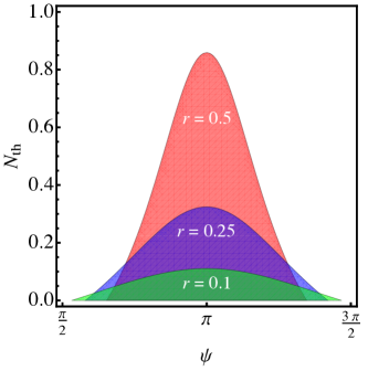
Figure 1: The threshold condition on the coherent amplitude of a single-mode Gaussian state to have $g^{(2)}_{\rm sGs}(0)<1$. The shaded areas (each one corresponding to a different value of the squeezing parameter $r$) are the regions of the $\psi$–$N_{\rm th}$ plane where a threshold $\alpha_{\rm Th}(r,\psi,N_{\rm th})$ exists. For values of $\psi$ and $N_{\rm th}$ outside those regions we have $g^{(2)}_{\rm sGs}(0)>1$.

In Fig. 1, we show the regions of the $\psi$–$N_{\rm th}$ plane where this positivity condition is satisfied. When $\alpha_{\rm Th}(r,\psi,N_{\rm th})$ exists, we have (for a given set of parameters $\{r,\psi,N_{\rm th}$) that $g^{(2)}_{\rm sGs}(0)<1$ if $\alpha>\alpha_{\rm Th}(r,\psi,N_{\rm th})$ and vice versa. If, on the other hand, the threshold does not exists, then the second-order correlation function is always greater than 1. The threshold, for a given $r$, may exist only if $\pi/2\leq\psi\leq 3\pi/2$ and, as the value of $r$ increases, the shaded region becomes more and more peaked around $\psi=\pi$ (see Fig. 1).

It is worth noting that for $\psi=\pi$ (amplitude squeezing), Eq. (19) reduces to:

$$\alpha_{\rm Th}(r,\pi,N_{\rm th})=$$

$$\frac{1}{2}\sqrt{\frac{(1+2N_{\rm th})^{2}\sinh^{2}(2r)+\left[(1+2N_{\rm th})\cosh(2r)-1\right]^{2}}{{\cal T}(r,N_{\rm th})}}\,,$$ (20)

therefore, in the presence of amplitude squeezing and real displacement, the zero-delay second-order correlation function can be less the 1 iff the state is nonclassical, namely, exhibits a non-null nonclassical depth ${\cal T}(r,N_{\rm th})$. Otherwise, $\alpha_{\rm Th}(r,\pi,N_{\rm th})$ does not exist (we recall that, according to our choice of the parameters, this threshold should be real). In the this case ($\psi=\pi$), the minimum (if exists!) occurs at (see also [20, 31]):

$$\alpha_{\rm min}(r,\pi,N_{\rm th}) =\sqrt{(1+2N_{\rm th})\sinh(2r)}$$

$$\hskip 28.45274pt\times\sqrt{\frac{(1+2N_{\rm th})\sinh(2r)}{{\cal T}(r,N_{\rm th})}-\frac{1}{2}}\,.$$ (21)

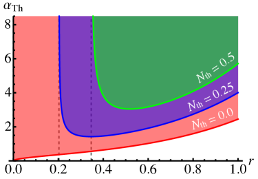
Figure 2: The threshold on the amplitude $\alpha_{\rm Th}(r,\pi,N_{\rm th})$ (for $\psi=\pi$) as a function of $r$ for different values of $N_{\rm th}$. In the shaded regions $g^{(2)}_{\rm sGs}(0)<1$. The dashed vertical lines correspond to $r_{\rm Th}(N_{\rm th})=\frac{1}{2}\log(1+2N_{\rm th})$: if $r\leq r_{\rm Th}(N_{\rm th})$ the single-mode Gaussian state is classical (it has zero nonclassical depth) and $\alpha_{\rm Th}$ does not exist.

In Fig. 2 we plot the threshold $\alpha_{\rm Th}(r,\pi,N_{\rm th})$ and highlight the regions in which $g^{(2)}_{\rm sGs}(0)<1$: we can see that as the value of $N_{\rm th}$ increases, thus reducing the purity $\mu[\varrho]=(1+2N_{\rm th})^{-1}$ of the state (16), $\alpha_{\rm Th}(r,\pi,N_{\rm th})$ increases as well.

3.2 Two-mode Gaussian states

Now we consider the second-order correlation function of two-mode Gaussian states, which, using Eqs. (4), can be written as:

$$g^{(2)}_{\rm TM}(0)= \frac{\langle\hat{a}^{{\dagger}}\hat{a}^{{\dagger}}\hat{a}\hat{a}\rangle+\langle\hat{b}^{{\dagger}}\hat{b}^{{\dagger}}\hat{b}\hat{b}\rangle+2\langle\hat{a}^{{\dagger}}\hat{a}\,\hat{b}^{{\dagger}}\hat{b}\rangle}{\left(\langle\hat{a}^{{\dagger}}\hat{a}\rangle+\langle\hat{b}^{{\dagger}}\hat{b}\rangle\right)^{2}}\,$$ (22a)

$$= \,\frac{\langle[(\hat{a}^{\dagger})^{2}\hat{a}^{2}]_{\rm s}\rangle+\langle[(\hat{b}^{\dagger})^{2}\hat{b}^{2}]_{\rm s}\rangle}{\left[\langle[(\hat{a}^{\dagger})\hat{a}]_{\rm s}\rangle+\langle[(\hat{b}^{\dagger})\hat{b}]_{\rm s}\rangle-1\right]^{2}}$$

$$\hskip 14.22636pt-\frac{3\left(\langle[\hat{a}^{\dagger}\hat{a}]_{\rm s}\rangle+\langle[\hat{b}^{\dagger}\hat{b}]_{\rm s}\rangle-\frac{1}{2}\right)}{\left[\langle[(\hat{a}^{\dagger})\hat{a}]_{\rm s}\rangle+\langle[(\hat{b}^{\dagger})\hat{b}]_{\rm s}\rangle-1\right]^{2}}$$

$$\hskip 14.22636pt+\frac{2\langle[\hat{a}^{\dagger}\hat{a}]_{\rm s}[\hat{b}^{\dagger}\hat{b}]_{\rm s}\rangle}{\left[\langle[(\hat{a}^{\dagger})\hat{a}]_{\rm s}\rangle+\langle[(\hat{b}^{\dagger})\hat{b}]_{\rm s}\rangle-1\right]^{2}}\,,$$ (22b)

where $\hat{a}=\hat{a}_{1}$ and $\hat{b}=\hat{a}_{2}$ are the two involved modes. Here, for the sake of clarity, we restrict or analysis to the class of the two-mode squeezed thermal states (TMSTS) which we can generate and manipulate with the current technology [21, 27]. The density operator associated with a TMSTS can be written as:

$$\varrho_{ab}=D_{ab}(\alpha,\beta)\,S_{2}(\xi)\ \nu_{a}(N_{\rm th,1})\otimes\nu_{b}(N_{\rm th,2})\,S_{2}^{{\dagger}}(\xi)D_{ab}^{{\dagger}}(\alpha,\beta)\,,$$ (23)

where $D_{ab}(\alpha,\beta)=D_{a}(\alpha)\otimes D_{b}(\beta)$, with $D_{k}(z)=\exp(z\hat{k}^{\dagger}-z^{*}\hat{k})$, $S_{2}(\xi)=\exp(\xi\hat{a}^{\dagger}\hat{b}^{\dagger}-\xi^{*}\hat{a}\hat{b})$ is the two-mode squeezing operator ($\xi=r\,e^{i\psi}$ is now the two-mode squeezing parameter) and $\nu_{k}(N)=N^{\hat{k}^{\dagger}\hat{k}}/(1+N)^{\hat{k}^{\dagger}\hat{k}+1}$ is the “thermal” state of mode $\hat{k}$ with $N$ mean photons. The corresponding $4\times 4$ CM has the following block matrix form [4]:

$$\boldsymbol{\sigma}=\frac{1}{2}\left(\begin{array}[]{cc}A\,\mathbb{I}_{2}&C\,\boldsymbol{R}_{\xi}\\[4.30554pt] C\,\boldsymbol{R}_{\xi}&B\,\mathbb{I}_{2}\end{array}\right)$$ (24)

where $\mathbb{I}$ is the $2\times 2$ identity matrix,

$$\boldsymbol{R}_{\xi}=\sinh r\,\left(\begin{array}[]{cc}\cos\psi&\sin\psi\\[4.30554pt] \sin\psi&-\cos\psi\end{array}\right)$$ (25)

and:

$$A =\cosh(2r)+2\left(N_{\rm th,1}\cosh^{2}r+N_{\rm th,2}\sinh^{2}r\right)\,,$$ (26a)

$$B =\cosh(2r)+2\left(N_{\rm th,1}\sinh^{2}r+N_{\rm th,2}\cosh^{2}r\right)\,,$$ (26b)

$$C =(1+N_{\rm th,1}+N_{\rm th,2})\sinh(2r)\,.$$ (26c)

Given the CM (24) it is straightforward to calculate the second-order correlation function $g^{(2)}_{\rm TM}(0)$ of the corresponding state $\varrho_{ab}$ in Eq. (23). The analytical formula is clumsy and it is not reported explicitly in its general form. However, the results are similar to those obtained in the case of the single-mode Gaussian states discussed above. In particular, if we set $\psi=\pi$ we can still find the threshold values of the coherent amplitudes $\alpha$ and $\beta$ and of the thermal contributions $N_{\rm th,1}$ and $N_{\rm th,2}$, in order to have $g^{(2)}_{\rm TM}<1$. This is not possible if we choose $\psi=0$ instead.

Figure 3: Contour plot of the the second-order correlation function $g^{(2)}_{\rm TM}$ of two-mode Gaussian states as a function of the displacement amplitudes $\alpha$ and $\beta$ in the case of the TMSTS given in Eq. (23) with $N_{\rm th,1}=N_{\rm th,2}=0$ (left panel) and $N_{\rm th,1}=N_{\rm th,2}=0.15$ (right panel). In both the panels we set $r=0.5$ and $\psi=\pi$, where $\xi=r\,e^{i\psi}$ is the two-mode squeezing parameter, see the text for details. Only the region for $g^{(2)}_{\rm TM}<1$ is shown (note that for $\psi=0$ one has $g^{(2)}_{\rm TM}>1$, $\forall\alpha,\beta\geq 0$).

In Fig. 3 we report the region of the plane $(\alpha,\beta)$ leading to $g^{(2)}_{\rm TM}<1$ for two values of the thermal contribution (for the sake of simplicity we set $N_{\rm th,1}=N_{\rm th,2}$) and $r=0.5$ (with $\psi=\pi$, as mentioned above) that is a typical value we can easily reach in the experiments. Figure 4 shows the region of the plane $(N_{\rm th,1},N_{\rm th,2})$ for which $g^{(2)}_{\rm TM}<1$ when we fix $\alpha=\beta=2$ and use two values of the two-mode squeezing parameter (its phase $\psi$ is still set equal to $\pi$).

Figure 4: Contour plot of the the second-order correlation function $g^{(2)}_{\rm TM}$ of two-mode Gaussian states as a function of the thermal contributions $N_{\rm th,1}$ and $N_{\rm th,2}$ in the case of the TMSTS given in Eq. (23) with $\alpha=\beta=2$ and two-mode squeezing parameter $r=0.5$ (left panel) and $r=0.2$ (right panel), where $\xi=r\,e^{i\psi}$ and we set $\psi=\pi$ in both the panels, see the text for details. Only the region for $g^{(2)}_{\rm TM}<1$ is shown (note that for $\psi=0$ one has $g^{(2)}_{\rm TM}>1$, $\forall N_{\rm th,1},N_{\rm th,2}\geq 0$).

From the Figs. 3 and 4 its is clear that the best working regime is obtained in the presence of a symmetric configuration, namely, for $\alpha=\beta$ and $N_{\rm th,1}=N_{\rm th,2}$. This is usually the regime achieved in actual experiments involving sideband modes [27]. In this case, it is possible to write a more compact analytical expression for the two-mode second-order correlation function and we can find the following threshold of $\alpha$ such that $g^{(2)}_{\rm TM}(0)=1$, namely:

$$\tilde{\alpha}_{\rm Th}(r,\psi,N_{\rm th})=$$

$$\frac{1}{2}\sqrt{\frac{(1+2N_{\rm th})^{2}\sinh^{2}(2r)+\left[(1+2N_{\rm th})\cosh(2r)-1\right]^{2}}{\frac{1}{2}\left[{\cal T}(r,N_{\rm th})+{\cal T}(-r,N_{\rm th})\right]-(1+2N_{\rm th})\sinh(2r)\cos\psi}}\,,$$ (27)

where ${\cal T}(\pm r,N_{\rm th})$ was introduced in Eq. (19). Note that for $\psi=\pi$, the threshold $\tilde{\alpha}_{\rm Th}(r,\pi,N_{\rm th})$ reduces to the same threshold obtained for the single-mode Gaussian states given in Eq. (20).

Up to now, we have studied $g^{(2)}(0)$ as a function of the relevant parameters characterising the single- or two-mode Gaussian state under investigation. However, if we focus on the single-mode states, thanks to Eqs. (11a) and (12) we can retrieve the value of $g^{(2)}_{\rm sGs}(0)$ by acquiring the information about the covariance matrix and the first moment vector. These quantities straightforwardly follow from the measurement of the four quadratures $\hat{q}$, $\hat{p}$ and $\hat{x}_{\pm\pi/4}$ as mentioned in the section 2 and they can be experimentally obtained by a single homodyne detector, as we are going to demonstrate in the next section. Similar results can be obtained for two-mode Gaussian states [15, 27], and they are worth to be thoroughly investigated in future works.

4 Experimental apparatus and single-mode state results

In order to test the theoretical previsions, we built an experimental setup to generate and manipulate displaced-squeezed states. In particular, our scheme allows controlling both the coherent amplitude and the squeezing parameter of the states as well as their relative phase. Therefore we can process the two families of amplitude and phase squeezed states.

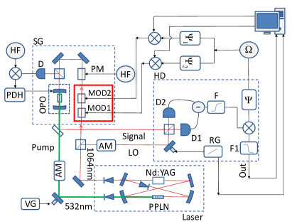
Figure 5: (Color online) Schematic diagram of the experimental setup to generate squeezed states. The principal radiation source is provided by a home made Nd:YAG Laser internally-frequency-doubled. One laser output (@ 532 nm) pumps the MgO:LiNbO₃ crystal (length 10 mm) of the optical parametric oscillator (OPO) whereas the other output (@ 1064 nm) is sent to a polarising beam splitter to generate the local oscillator (LO) as well as the seed signal for the OPO. The power of the LO is set by an amplitude modulator (AM). The phase modulators (PM) generates the sidebands @ 110 MHz for the active stabilisation of the OPO cavity. Whereas the two modulators (MOD1, MOD2) generate the sidebands @ 3 MHz for the seed state generation, in particular by exploiting these two modulators we can set the values of $\alpha$ and $\psi$ by the computer. The length of the OPO cavity is actively controlled by a piezo connected to its rear mirror. The homodyne detector consists of a 50:50 beam splitter, two low noise detectors (D1, D2) and a differential amplifier. The relative phase between the pump @ 532 nm and the radiation @ 1064 nm is set by a piezo connected with a voltage generator (VG).

Figure 5 shows the scheme of our experimental apparatus. It consists of three stages: Laser, signal generator (SG) and homodyne detector (HD) (see more details in [38]). In particular continuous-wave squeezed light is generated by a sub-threshold optical parametric oscillator (OPO). The OPO input seed (1064 nm) and the OPO pump beam (532 nm) arise from a home-made internally frequency doubled Nd:YAG laser. The output at 1064 nm is split into two beams by using a polarising beam splitter (PBS): one is used as the local oscillator (LO) for the homodyne detector and the other is sent into the OPO. A phase modulator (PM) generates a signal at frequency of 110 MHz (HF) used as active stabilisation of the OPO cavity via the Pound-Drever-Hall (PDH) technique [27]. In order to generate the coherent squeezed states our strategy is to exploit the combined effect of two optical modulators (MOD1, MOD2) placed before the OPO. By properly chosen the modulation amplitudes [38], it is possible to generate arbitrary coherent states on the sidebands @ 3 MHz for seeding the OPO [27, 38]. In this way we can set both the value of the phase $\psi$ and the value of $\alpha$ on demand by the computer.

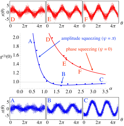
Figure 6: Experimental $g^{(2)}_{\rm sGs}(0)$ (dots) obtained through Eq. (15c) in the case of amplitude ($r=0.5\pm 0.05$ and $N_{\rm th}=0.14\pm 0.04$) and phase squeezing ($r=0.46\pm 0.04$ and $N_{\rm th}=0.16\pm 0.03$) for different values of the (real) amplitude $\alpha$. The solid lines correspond to the theoretical previsions. The insets show the experimental homodyne traces processed in order to obtain the value of $g^{(2)}_{\rm sGs}(0)$ (marked with the corresponding capital letters) according to the theory presented in section 3.

After collecting the homodyne traces for a given state we first checked the Gaussianity of the input state by assessing the Kurtosis of the data sample as well as a more comphrensive battery of Gaussianity test [15, 39]. Then, we evaluated the needed expectations by using the pattern function tomography, which allows one to reconstruct the moments of a given quadratures upon exploiting the whole data sample, thus reducing the statistical errors. The results are reported in Fig. 6, where we show the experimentally obtained values of $g^{(2)}_{\rm sGs}(0)$ (dots) as a function of the displacement (real) amplitude $\alpha$ for both phase and amplitude squeezing together with the theoretical predictions (solid lines). According to the theoretical results, in the presence of amplitude squeezing we find a threshold on $\alpha$ above which $g^{(2)}_{\rm sGs}(0)<1$, whereas the phase squeezed states always lead to a positive second-order correlation function. In the same figure we also report the raw homodyne traces corresponding to some of the experimental points: features of amplitude squeezing (A, B and C) or phase squeezing (D, E and F) are clearly seen.

5 Conclusions

In conclusion, we have suggested and demonstrated a reconstruction scheme for the zero-delay-time second-order correlation function $g^{(2)}(0)$ of Gaussian states and we have proved it experimentally for single-mode states. Our scheme is based on a single homodyne detector and the quantum state reconstruction of Gaussian state by pattern function tomography. The results are based on the analytic expression of the correlation function $g^{(2)}(0)$ in terms of the elements of covariance matrix and the displacement amplitude of the Gaussian state, which also show that when the input state is nonclassical, there exists a threshold value of the coherent amplitude, and a range of values of the complex squeezing parameter, above which $g^{(2)}(0)<1$. For amplitude squeezing and real coherent amplitude, the threshold is a necessary and sufficient condition for the nonclassicality of the state. Our technique allows us to reliably characterise photon-number nonclassicality of Gaussian states without the need of photon-resolving detectors. Eventually, the recent achievements we obtained in the experimental reconstruction of symmetric two-mode squeezed thermal states [27] pave the way for further investigation of the second-order correlation function beyond the single-mode case, which will be thoroughly addressed in future works.

References

References

• [1] S. Olivares, Quantum optics in the phase space, Eur. Phys. J. Special Topics 203, 3-24 (2012)
• [2] C. Weedbrook, S. Pirandola, R. García-Patrón, N. J. Cerf, T. C. Ralph, J. H. Shapiro, and S. Lloyd, Gaussian quantum information, Rev. Mod. Phys. 84, 621-669 (2012).
• [3] G. Adesso, S. Ragy, and A. R. Lee, Continuous Variable Quantum Information: Gaussian States and Beyond, Open Syst. Inf. Dyn. 21, 1440001 (2014).
• [4] A. Ferraro, S. Olivares and M. G. A. Paris, Gaussian States in Quantum Information (Bibliopolis, Napoli, 2005).
• [5] S. Olivares, High-precision innovative sensing with continuous-variable optical states, Riv. Nuovo Cim. 41, 341-382 (2018).
• [6] H. P. Yuen, and W. S. Chan, Noise in homodyne and heterodyne detection, Opt.Lett. 8,177 (1983).
• [7] B. L. Schumaker, Noise in homodyne detection, Opt.Lett. 9, 189 (1984).
• [8] A. Zavatta, M. Bellini, P. L. Ramazza, F. Marin, and F. T. Arecchi, Time-domain analysis of quantum states of light: noise characterization and homodyne tomography , J. Opt. Soc. Am. B 19, 1189 (2002).
• [9] S. Grandi, A. Zavatta, M. Bellini, M. G. A. Paris, Experimental quantum tomography of a homodyne detector, New J. Phys. 19, 053015 (2017).
• [10] L. S. Madsen, A. Berni, M. Lassen, and U. L. Andersen, Experimental investigation of the evolution of Gaussian quantum discord in an open system, Phys. Rev. Lett. 109, 030402 (2012).
• [11] R. Blandino, M. G. Genoni, J. Etesse, M. Barbieri, M. G. A. Paris, P. Grangier, R. Tualle-Brouri, Homodyne estimation of Gaussian quantum discord, Phys. Rev. Lett 109, 180402 (2012).
• [12] V. Chille, N. Quinn, C. Peuntinger, C. Croal, L. Mista, Jr., Ch. Marquardt, G. Leuchs, N. Korolkova, Quantum nature of Gaussian discord: Experimental evidence and role of system-environment correlations, Phys. Rev. A 91, 050301(R) (2015).
• [13] G. M. D’Ariano, M. G. A. Paris, and M. F. Sacchi, Quantum tomography, Advances in Imaging and Electron Physics 128, 206-309 (Academic Press, 2003); G. M. d’Ariano, C Macchiavello, M. G. A Paris, Phys. Letters A 195, 31 (1994).
• [14] M. Esposito, F. Benatti, R. Floreanini, S. Olivares, F. Randi, K. Titimbo, M. Pividori, F. Novelli, F. Cilento, F. Parmigiani, and D. Fausti, Pulsed homodyne Gaussian quantum tomography with low detection efficiency, New. J. Phys. 16, 043004 (15 pages) (2014).
• [15] D. Buono, G. Nocerino, V. D’Auria, A. Porzio, S. Olivares, and M. G. A. Paris, Quantum characterization of bipartite Gaussian states, J. Opt. Soc. Am. B 27, A110-A118 (2010).
• [16] A. Serafini, F. Illuminati, and S. De Siena, Symplectic invariants, entropic measures and correlations of Gaussian states, J. Phys. B: At. Mol. Opt. Phys. 37, L21-L28 (2004).
• [17] Z. Hradil, J. Rehacek, J. Fiurasek, M. Jezek, Maximum-Likelihood Methods in Quantum Mechanics, Lect. Notes Phys. 649, 59?112 (2004).
• [18] J. Park, S.-W. Ji, J. Lee, and H. Nha Gaussian states under coarse-grained continuous variable measurements, Phys. Rev. A 89, 042102 (2014).
• [19] R. Glauber, Nobel lecture: 100 years of light quanta, Rev. Mod. Phys. 78, 1267 (2006).
• [20] M. Alexanian, Temporal second-order coherence function for displaced-squeezed thermal states, J. Mod. Opt. 63, 961 (2016).
• [21] V. D’Auria, S. Fornaro, A. Porzio, S. Solimeno, S. Olivares and M. G. A. Paris, Full characterization of Gaussian bipartite entangled states by a single homodyne detector, Phys. Rev. Lett. 102, 020502 (2009).
• [22] B. Qi, P. Lougovski, and B. P. Williams, Characterizing photon number statistics using conjugate optical homodyne detection, eprint arXiv:1702.02558 [quant-ph].
• [23] Y. S. Teo, C. R. Muller, H. Jeong, Z. Hradil, J. Rehacek, and L. L. Sanchez-Soto, Superiority of heterodyning over homodyning: An assessment with quadrature moments, Phys. Rev. A 95, 042322 (2017).
• [24] A. Allevi, S. Olivares, and M. Bondani, Measuring high-order photon-number correlations in experiments with multimode pulsed quantum states Phys. Rev. A 85, 063835 (2012).
• [25] M. Bina, and S. Olivares, Intensity correlations from linear interactions, Quantum Meas. Quantum Metrol. 2, 50 (2014).
• [26] F. A. S. Barbosa, A. S. Coelho, K. N. Cassemiro, P. Nussenzveig, C. Fabre, A. S. Villar, and M. Martinelli, Quantum state reconstruction of spectral field modes: Homodyne and resonator detection schemes, Phys. Rev. A 88, 052113 (2013)
• [27] S. Cialdi, C. Porto, D. Cipriani, S. Olivares, and M. G. A. Paris, Full quantum state reconstruction of symmetric two-mode squeezed thermal states via spectral homodyne detection and a state-balancing detector, Phys. Rev. A 93, 043805 (2016).
• [28] I. Ruo Berchera, I. P. Degiovanni, S. Olivares, N. Samantaray, P. Traina, and M. Genovese, One- and two-mode squeezed light in correlated interferometry, Phys. Rev. A 92, 053821 (2015).
• [29] C. Sparaciari, S. Olivares, and M. G. A. Paris, Bounds to precision for quantum interferometry with Gaussian states and operations, J. Opt. Soc. Am. B 32, 1354-1359 (2015); Phys. Rev. A 93, 023810 (2016).
• [30] I. Ruo Berchera, I. P. Degiovanni, S. Olivares, and M. Genovese Quantum light in coupled interferometers for quantum gravity tests, Phys. Rev. Lett. 110, 213601 (2013).
• [31] J. S. Pedernales, R. Di Candia, I. L. Egusquiza, J. Casanova, and E. Solano, Efficient Quantum Algorithm for Computing n-time Correlation Functions, Phys. Rev. Lett. 113, 020505 (2014).
• [32] E. D. Lopaeva, I. Ruo Berchera, I. P. Degiovanni, S. Olivares, G. Brida, and M. Genovese, Experimental realization of quantum illumination, Phys. Rev. Lett. 110, 153603 (2013).
• [33] K. E. Cahill and R. J. Glauber, Ordered Expansions in Boson Amplitude Operators, Phys. Rev. 77, 1857 (1969).
• [34] G. Adam, Density Matrix Elements and Moments for Generalized Gaussian State Fields, J. Mod. Opt. 42, 1311-1328 (1995).
• [35] C. T. Lee, Measure of the nonclassicality of nonclassical states, Phys. Rev. A 44, R2775 (1991).
• [36] M. Brunelli, C. Benedetti, S. Olivares, A. Ferraro and M. G. A. Paris, Single- and two-mode quantumness at a beam splitter, Phys. Rev. A 91, 062315 (2015).
• [37] S. Olivares and M. G. A. Paris, Optimized interferometry with Gaussian states, Opt. Spectrosc. 103, 231 (2007).
• [38] A. Mandarino, M. Bina, C. Porto, S. Cialdi, S. Olivares, M. G. A. Paris, Assessing the significance of fidelity as a figure of merit in quantum state reconstruction of discrete and continuous variable systems, Phys. Rev. A 93, 062118 (2016).
• [39] J. Řeháček, S. Olivares, D. Mogilevtsev, Z. Hradil, M. G. A. Paris, S. Fornaro, V. D’Auria, A. Porzio, S. Solimeno, Effective method to estimate multidimensional Gaussian states, Phys. Rev. A 79, 032111 (2009).