Bulk View of Teleportation and Traversable Wormholes

Dongsu Bak,${}^{\,\tt a}$ Chanju Kim,${}^{\,\tt b}$ Sang-Heon Yi${}^{\,\tt a}$

a) Physics Department, University of Seoul, Seoul 02504 KOREA

b) Department of Physics, Ewha Womans University, Seoul 03760 KOREA

(dsbak@uos.ac.kr, cjkim@ewha.ac.kr, shyi704@uos.ac.kr)

ABSTRACT

We construct detailed AdS₂ gravity solutions describing the teleportation through a traversable wormhole sending a state from one side of the wormhole to the other. The traversable wormhole is realized by turning on a double trace interaction that couples the two boundaries of an eternal AdS₂ black hole. The horizon radius or the entropy of the black hole is reduced consistently with the boundary computation of the energy change, confirming the black hole first law. To describe teleportee states traveling through the wormhole, we construct Janus deformations which make the Hamiltonians of left-right boundaries differ from each other by turning on exact marginal operators. Combining explicitly the traversable wormhole solution and the teleportee states, we present a complete bulk picture of the teleportation in the context of ER=EPR. The traversability of the wormhole is not lost to the leading order of the deformation parameter. We also consider solutions where the teleportee meets the matter thrown from the other side during teleportation, in accordance with the assertion that the bulk wormhole is experimentally observable.

1 Introduction

There are some renewed interests in AdS₂ space, inspired by the proposal for its correspondence with the four-Fermi random interaction model, known as the SYK model [1] (See [2] for a review). Historically, AdS₂ space has received the attention as the essential part in the near horizon of the extremal black holes. Since the temperature of extremal black holes vanishes and those black holes do not emit the Hawking radiation, those are regarded as stable objects with mass gap, providing an ideal test ground for various methodologies of the microscopic counting of black hole entropy. One might anticipate the concrete realization of ideas or analytic computations on black holes in the context of AdS₂/CFT₁ correspondence. On the contrary, it turns out to be a bit twisted to construct a meaningful gravity theory on two-dimensional spacetime, since pure Einstein theory becomes topological on two dimensions. Recent developments in the correspondence utilize the freedom in the boundary degrees in the two-dimensional gravity, and so the nearly-AdS₂ space is taken as the bulk background.

Another interesting aspect of AdS₂ space is that it has two boundaries different from the single boundary in its higher dimensional cousins, which may put a hurdle on the direct adaptation of methods in higher dimensional case. However, even in higher dimensional AdS case, it has been known that the eternal AdS black holes provide two boundaries and can naturally be identified with the highly-entangled, so-called, thermo field double states (TFD) in the finite temperature field theory [3, 4]. Recently, this aspect of the existence of two boundaries in eternal AdS black holes and its correspondence with TFD has led to an interesting bulk realization of quantum teleportation: traversable wormhole [5, 6, 7, 8, 9, 10]. By turning on the double trace interaction between two boundaries with a negative energy, it is explicitly shown that the average null-energy condition in the bulk is violated and so wormholes could be traversable. This bulk geometry is argued to be interpreted as the gravity realization of the quantum teleportation in the dual theory. Though the turned-on interaction between two boundaries is taken to be very small admitting its perturbative treatment, it is argued that the bulk deformation caused by the back-reaction renders wormholes as traversable ones.

In this paper, we consider the two-dimensional Einstein-dilaton model with a scalar field and investigate the concrete bulk dilaton dynamics. In this model, one can show by the explicit computation that the dilaton dynamics by the boundary interaction cause the position of the singularity of black holes is moved in a way that the wormhole becomes traversable. One can also show that the horizon radius or the entropy of black holes is reduced consistently with the black hole 1st law. Furthermore, we consider the thermalization and Janus deformation of black holes and show that it could be combined with the two boundary interaction consistently. This could be regarded as the complete bulk realization of the quantum teleportation.

Although this bulk description can be made fully consistent in its own right, there is in general an extra back-reaction effect in identification of its corresponding boundary system. Once there are any excitations from an AdS₂ black hole, identification of the left-right (L-R) boundary time coordinates $t_{L/R}$ as a function of the bulk time coordinate $t$ at regulated L-R boundaries becomes nontrivial. Without any excitations above the thermal vacuum, one has simply $t(t_{L/R})=t_{L/R}$. On the other hand, if the system is excited, this (reparameterization) dynamics becomes nontrivial as was emphasized in Ref. [11]. In this note, we shall show the consistency of our bulk description with that of the boundary side only to the leading order. Of course the full identification of the correspondence requires the formulation introduced in Ref. [11], which we shall not attempt to do in this note. See also Refs. [8, 10] for the account of teleportation in this direction.

This paper is organized as follows. In Section 2, we present our model and summarize basic black hole solutions and their basic properties. In Section 3, we consider the scalar field perturbation of black holes and its thermalization. In Section 4, we provide a specific time-dependent Janus deformation of AdS₂ black holes and show that one cannot send signal from one boundary to the other in this case. In Sections 5 and 6, we consider the double trace deformation between two boundaries and show that it renders the wormhole to be traversable with the explicit entropy/temperature reduction. In Section 7, we combine our results in previous sections and provide the complete bulk picture dual to the quantum teleportation. We conclude in Section 8 with some discussion. Various formulae are relegated to Appendices.

2 Two-dimensional dilaton gravity

We begin with the 2d dilaton gravity in Euclidean space [12, 13, 14]

$$I=I_{top}-{1\over 16\pi G}\int_{M}d^{2}x\sqrt{g}\,\phi\left(R+\frac{2}{\ell^{2}}\right)+I_{M}(g,\chi)\,,$$ (2.1)

where

$$I_{top} =-{\phi_{0}\over 16\pi G}\int_{M}d^{2}x\sqrt{g}R\,,$$

$$I_{M} =\frac{1}{2}\int_{M}d^{2}x\sqrt{g}\left(\nabla\chi\cdot\nabla\chi+m^{2}\chi^{2}\right)\,.$$ (2.2)

Below we shall evaluate the above action on shell, which would diverge if the boundary is taken at infinity. For its regularization, we introduce a cutoff surface $\partial M$ near infinity. This requires adding surface terms

$$I_{surf}=-{1\over 8\pi G}\int_{\partial M}\sqrt{\gamma}\,(\phi_{0}+\phi)\,K\,,$$ (2.3)

where $\gamma_{ij}$ and $K$ denote the induced metric and the extrinsic curvature. Then the renormalized action (obtained by adding the counter terms) corresponds to the free energy multiplied by $\beta$,

$$I_{ren}=\beta F=-\log Z\,,$$ (2.4)

where $Z$ is the partition function of the dual quantum mechanical system.

The corresponding Lorentzian action takes the form

$$I=I_{top}+{1\over 16\pi G}\int_{M}d^{2}x\sqrt{-g}\,\phi\left(R+\frac{2}{\ell^{2}}\right)+I_{M}(g,\chi)\,,$$ (2.5)

where

$$I_{top} ={\phi_{0}\over 16\pi G}\int_{M}d^{2}x\sqrt{-g}\,R\,,$$

$$I_{M} =-\frac{1}{2}\int_{M}d^{2}x\sqrt{-g}\left(\nabla\chi\cdot\nabla\chi+m^{2}\chi^{2}\right)\,.$$ (2.6)

The equations of motion read

$$R+\frac{2}{\ell^{2}}=0\,,$$

$$\nabla^{2}\chi-m^{2}\chi=0\,,$$

$$\nabla_{a}\nabla_{b}\phi-g_{ab}\nabla^{2}\phi+g_{ab}\phi=-8\pi GT_{ab}\,,$$ (2.7)

where

$$T_{ab}=\nabla_{a}\chi\nabla_{b}\chi-\frac{1}{2}g_{ab}\left(\nabla\chi\cdot\nabla\chi+m^{2}\chi^{2}\right)\,.$$ (2.8)

Any AdS₂ space can be realized by the global AdS space whose metric is given by

$$ds^{2}=\frac{\ell^{2}}{\cos^{2}\mu}\left(-d\tau^{2}+d\mu^{2}\right)\,,$$ (2.9)

where $\mu$ is ranged over $[-\frac{\pi}{2},\frac{\pi}{2}]$. The most general vacuum solution for the dilaton field is given by

$$\phi=\frac{1}{\cos\mu}\left(\alpha_{0}\cos\tau+\alpha_{1}\sin\tau\right)+\alpha_{2}\frac{\sin\mu}{\cos\mu}\,.$$ (2.10)

Using the translational isometry along $\tau$ direction, one may set $\alpha_{1}$ to zero without loss of generality. We shall parameterize the dilaton field by

$$\phi=\phi_{BH}(L,b,\tau_{B})\equiv\bar{\phi}\,L\,\,\frac{(b+b^{-1})\cos(\tau-\tau_{B})-(b-b^{-1})\sin\mu}{2\cos\mu}\,,$$ (2.11)

where we choose $b\geq 0$. By the coordinate transformation

$$\frac{r}{L} =\frac{(b+b^{-1})\cos(\tau-\tau_{B})-(b-b^{-1})\sin\mu}{2\cos\mu}\,,$$

$$\tanh\frac{tL}{\ell^{2}} =\frac{2\sin(\tau-\tau_{B})}{(b+b^{-1})\sin\mu-(b-b^{-1})\cos(\tau-\tau_{B})}\,,$$ (2.12)

one is led to the corresponding AdS black hole metric

$$ds^{2}=-\frac{r^{2}-L^{2}}{\ell^{2}}dt^{2}+\frac{\ell^{2}}{r^{2}-L^{2}}dr^{2}\,,$$ (2.13)

with

$$\phi=\bar{\phi}\,r\,.$$ (2.14)

The Penrose diagram for the above black hole with $b=1$ is depicted in Figure 1. They in general describe two-sided AdS black holes. The location of singularity is defined by the curve $\Phi^{2}\equiv\phi_{0}+\phi=0$ in the above dilaton gravity where $\Phi^{2}$ might be viewed as characterizing the size of “transverse space” [14]. In the figure, we set $\phi_{0}=0$ for definiteness.

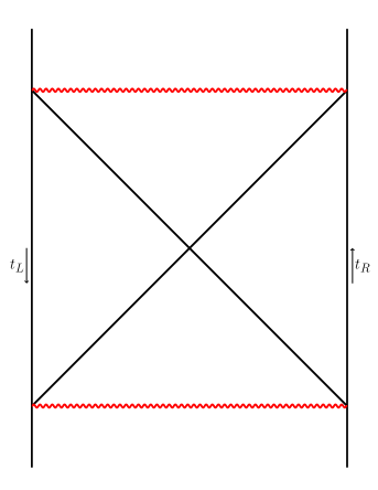
Figure 1: We draw the Penrose diagram for the AdS₂ black hole with $b=1$ in $(\tau,\mu)$ space where the wiggly red lines represent the location of singularity.

We now compute the free energy. For this, we go to the Euclidean space where the AdS solution read

$$ds^{2}=\frac{r^{2}-L^{2}}{\ell^{2}}dt_{E}^{2}+\frac{\ell^{2}}{r^{2}-L^{2}}dr^{2}$$ (2.15)

with

$$\phi=\bar{\phi}\,r\,.$$ (2.16)

The Gibbons-Hawking temperature can be identified as

$$T=\frac{1}{2\pi}\frac{L}{\ell^{2}}\,.$$ (2.17)

Note that the Euler number is defined by

$$\chi=\frac{1}{4\pi}\left[\,\int_{M}d^{2}x\sqrt{g}R+2\int_{\partial M}dx\sqrt{\gamma}K\,\right]\,,$$ (2.18)

which does not require any counter term. The (renormalized) topological term can be evaluated as

$$I^{top}_{ren}=-\frac{\phi_{0}}{4G}\,,$$ (2.19)

where we used the fact that $\chi=1$ for the thermal disk geometry. For the evaluation of the rest terms, we cutoff the bulk at

$$\frac{r}{L}=\frac{1}{\delta}\,.$$ (2.20)

Note that the second term in (2.1) is zero on-shell. Then the remaining term becomes

$$\Delta I_{reg}=-{1\over 8\pi G}\int_{\partial M}\sqrt{\gamma}\,\phi\,K=-\frac{\bar{\phi}}{8\pi G}\beta\frac{L^{2}}{\ell^{2}}\frac{1}{\delta^{2}}\,.$$ (2.21)

For the renormalization one has to go to the Fefferman-Graham coordinates. The metric in (2.15) becomes

$$ds^{2}=\frac{\ell^{2}}{z^{2}}dz^{2}+\frac{r^{2}(z)-L^{2}}{\ell^{2}}dt_{E}^{2}\,,$$ (2.22)

where

$$\frac{r}{L}=\frac{1+z^{2}}{2z}\,.$$ (2.23)

Therefore the cutoff $\epsilon$ in $z$ coordinate is related to $\delta$ by

$$\delta=\frac{2\epsilon}{1+\epsilon^{2}}\,,$$ (2.24)

and then

$$\Delta I_{reg}=-\frac{\bar{\phi}}{8\pi G}\beta\frac{L^{2}}{\ell^{2}}\frac{(1+\epsilon^{4}+2\epsilon^{2})}{4\epsilon^{2}}\,.$$ (2.25)

Subtracting the divergent term from $\Delta I_{reg}$ by a counter term $\sim\int_{z=\epsilon}\sqrt{\gamma}\,\phi$, one has

$$\Delta I_{ren}=-\frac{\bar{\phi}}{16\pi G}\beta\frac{L^{2}}{\ell^{2}}=-\frac{{\cal C}}{2}T\,,$$ (2.26)

where

$${\cal C}=\frac{\pi\bar{\phi}\ell^{2}}{2G}\,.$$ (2.27)

Thus the free energy becomes

$$F=-S_{0}T-\frac{{\cal C}}{2}T^{2}\,,$$ (2.28)

with

$$S_{0}=\frac{\phi_{0}}{4G}\,.$$ (2.29)

The entropy and energy are then

$$S =S_{0}+{\cal C}T\,,$$ (2.30)

$$E =\frac{1}{2}{\cal C}T^{2}\,.$$ (2.31)

We note that the deformation in $b$ does not play any role in the thermodynamics. In addition, note that the entropy can be written as a Beckenstein formula

$$S=\frac{\phi_{0}+\bar{\phi}\,L}{4G}\,.$$ (2.32)

As alluded earlier, we shall ignore the effect of $\phi_{0}$ by setting it to zero since we are not interested in this part of the black hole physics in the following. Below we shall focus on the $b=1$ case as our initial unperturbed system in constructing wormhole solutions. Of course, this can be relaxed to a general value of $b$.

The above two-sided black hole in the AdS₂ spacetime is dual to the so-called thermofield double [15] of CFT₁, which can be generalized to higher dimensions [4]. Without deformation of L-R coupling, the left and the right systems of $CFT_{L}\otimes CFT_{R}$ are decoupled from each other with Hamiltonians $H_{L}=H_{l}\otimes 1$ and $H_{R}=1\otimes H_{r}$ and the corresponding two time parameters $t_{L}$ and $t_{R}$, respectively. For the thermofield double of CFT, $H_{l}=H_{r}=H$ where $H$ is the Hamiltonian of a CFT. The left boundary time $t_{L}$ runs downward while $t_{R}$ runs upward in the AdS space. This identification is consistent with the coordinate system (2.12) since the orientation of time direction of $t$ in the left side is reversed from that of the right side. Since the orientation of $t_{L}$ is reverse to that of $t_{R}$, the time evolution of the full system is given by the operator $e^{iH_{L}t_{L}-iH_{R}t_{R}}$. When we view the full system embedded in a spacetime with extra dimensions with single time evolution, we may choose $t_{R}=-t_{L}=t$ with (undeformed) Hamiltonian

$$H_{tfd}=H_{L}+H_{R}=H\otimes 1+1\otimes H\,.$$ (2.33)

This single time evolution is also relevant when the left and the right systems are coupled, which is indeed the case with our teleportation protocol described below. The initial unperturbed thermal vacuum state is given by a particularly prepared entangled state [4]

$$|\Psi(0)\rangle=\frac{1}{\sqrt{Z}}\sum_{n,n^{\prime}}\,\langle n|{\cal U}|n^{\prime}\rangle\,|n^{\prime}\rangle\otimes|n\rangle=\frac{1}{\sqrt{Z}}\sum_{n}\,e^{-\frac{\beta}{2}E_{n}}\,|n\rangle\otimes|n\rangle\,,$$ (2.34)

with a Euclidean evolution operator ${\cal U}={\cal U}_{0}\equiv e^{-\frac{\beta}{2}H}$ and $Z$ denoting the normalization factor. The left-right entanglement here is maximal for a given temperature $T$.

3 Thermalization

In this section we shall construct various full back-reacted solutions describing thermalization of initial perturbations of black holes and investigate their general properties. It will be later on used to understand the dynamics of teleportee through the bulk. We will set $\ell=1$ in this and the next section.

In particular, we would like to solve the equations of motion in (2). The matter field $\chi$ with mass $m$ is dual to a scalar primary operator $O_{\Delta}(t)$, where its dimension is related to the mass by

$$\Delta=\frac{1}{2}\left(1+\sqrt{1+4m^{2}}\right)\,,$$ (3.1)

when $m^{2}\geq 0$. When $0>m^{2}>-1/4$, both possibilities of operator dimensions,

$$\Delta=\Delta_{\pm}=\frac{1}{2}\left(1\pm\sqrt{1+4m^{2}}\right)\,,$$ (3.2)

may be realized.

The scalar field equation can be solved by [16]

$$\chi=\sum^{\infty}_{n=0}c_{n}\,{\cal N}_{n}\cos^{\Delta}\mu\,C_{n}^{\Delta}(\sin\mu)\,e^{-i(n+\Delta)\tau}+{\rm c.c.}$$ (3.3)

where

$${\cal N}_{n}=2^{\Delta-1}\Gamma(\Delta)\sqrt{\frac{\Gamma(n+1)}{\pi\Gamma(n+2\Delta)}}\,,$$ (3.4)

and $C^{\Delta}_{n}(x)$ denotes the Gegenbauer polynomial defined in [17]. This bulk solution is dual to the deformation of thermofield initial state with a Euclidean evolution operator

$${\cal U}=e^{-\frac{\beta}{4}H}e^{-\sum_{n}c_{n}O_{n}^{\Delta}}e^{-\frac{\beta}{4}H}\,,$$ (3.5)

where we add a linear combination of operators $O_{n}^{\Delta}$ at the mid-point of the Euclidean evolution where $O_{n}^{\Delta}$’s denote the primary operator $O_{\Delta}$ and its descendants [18]. The Hamiltonian of the boundary system is undeformed on the other hand.

To see what this deformation describes, we need to look at the dilaton part whose identification will complete the fully back-reacted gravity solution of (2). Here we shall consider only $n=0$ case for the sake of an illustration. One may write the $n=0$ scalar solution as

$$\chi=\gamma\cos^{\Delta}\mu\cos\Delta(\tau+\tau_{C})\,,$$ (3.6)

without loss of generality. The corresponding dilaton solution can be found as

$$\phi =\bar{\phi}\,\tilde{L}\,\,\frac{(b+b^{-1})}{2}\frac{\cos\tau}{\cos\mu}-\frac{2\pi G\gamma^{2}\Delta}{1+2\Delta}\cos^{2\Delta}\mu\cos 2\Delta(\tau+\tau_{C})$$

$$~{}~{}~{}-2\pi G\gamma^{2}\Delta\cos^{2\Delta}\mu\,\,F\Big{(}\Delta,1\,;\,\frac{1}{2}\,\Big{|}\,\sin^{2}\mu\Big{)}\,,$$ (3.7)

where $\tilde{L}=L+\delta L$, $b=1+\delta b$ and $F(a,b\,;\,c\,|\,z)$ denotes the hypergeometric function [17]. We have added here a homogeneous solution that is consistent with the symmetry of the perturbation under $\mu\rightarrow-\mu$. To see its asymptotic structure in the region $\mu\rightarrow\pm\frac{\pi}{2}$, we shall use the following relation

$$F\Big{(}\Delta,1\,;\,\frac{1}{2}\,\Big{|}\,\sin^{2}\mu\Big{)}=\frac{1}{1+2\Delta}\,\,F\Big{(}\Delta,1\,;\,\Delta+\frac{3}{2}\,\Big{|}\,\cos^{2}\mu\Big{)}+\frac{\Gamma(\frac{1}{2})\Gamma(\Delta+\frac{1}{2})}{\Gamma(\Delta)\cos^{2\Delta}\mu}|\tan\mu|\,.$$ (3.8)

In the asymptotic region, the solution becomes

$$\phi=\bar{\phi}\,\tilde{L}\,\,\frac{(b+b^{-1})}{2}\frac{\cos\tau}{\cos\mu}-2\pi G\gamma^{2}\frac{\Delta\Gamma(\frac{1}{2})\Gamma(\Delta+\frac{1}{2})}{\Gamma(\Delta)}\frac{|\sin\mu|}{\cos\mu}+{\cal O}(\cos^{2\Delta}\mu)\,,$$ (3.9)

which will be compared to the black hole solution (2.11). This black hole is symmetric under the exchange of the left and the right as illustrated in Figure 2. The new temperature of the system is given by

$$\tilde{T}=\frac{1}{2\pi}\frac{\tilde{L}}{\ell^{2}}\,,$$ (3.10)

and the parameter $b$ on the right side can be determined by

$$\frac{b-b^{-1}}{2}=\frac{2\pi G\gamma^{2}}{\bar{\phi}\tilde{L}}\frac{\Delta\Gamma(\frac{1}{2})\Gamma(\Delta+\frac{1}{2})}{\Gamma(\Delta)}\,,$$ (3.11)

leading to

$$\delta b=\frac{2\pi G\gamma^{2}}{\bar{\phi}L}\frac{\Delta\Gamma(\frac{1}{2})\Gamma(\Delta+\frac{1}{2})}{\Gamma(\Delta)}+{\cal O}(G^{2}\gamma^{4})\,,$$ (3.12)

where we assume that $\delta L$ is of order $G\gamma^{2}$. Finally the shifts of the singularity in $\tau$ coordinate at the L-R boundaries can be identified as

$$\delta\tau_{L}^{\pm}=\delta\tau_{R}^{\pm} =\mp\arcsin\left[\frac{4\pi G\gamma^{2}}{\bar{\phi}\tilde{L}(b+b^{-1})}\frac{\Delta\Gamma(\frac{1}{2})\Gamma(\Delta+\frac{1}{2})}{\Gamma(\Delta)}\right]$$

$$=\mp\frac{2\pi G\gamma^{2}}{\bar{\phi}L}\frac{\Delta\Gamma(\frac{1}{2})\Gamma(\Delta+\frac{1}{2})}{\Gamma(\Delta)}+{\cal O}(G^{2}\gamma^{4})\,,$$ (3.13)

where $+/-$ respectively denotes the upper/lower singularities in the Penrose diagram. Therefore as illustrated in Figure 2, the corresponding Penrose diagram is given roughly by a rectangular shape where the length of the horizontal side is larger than the vertical size. Hence the right side is causally further away from the left side and of course the L-R boundaries are causally disconnected from each other completely. As will be illustrated further below explicitly, the vev of operators $\langle O_{\Delta}(t)\rangle_{R}$ can be identified. Here and below, $L/R$ in the expectation value represents that the operator of interest is acting on the left/right side Hilbert space. One finds in general that any initial perturbations of states will decay away exponentially in time. As was noted previously for the other dimensions [18], these solutions are describing thermalization of excited states above the thermal vacuum. This late-time exponential decay implies that the classical gravity description is inevitably coarse-grained [18], whose nature in the context of the AdS/CFT correspondence is explored in [19].

Figure 2: We depict the deformation of the Penrose diagram with initial perturbation of thermal vacuum.

3.1 $\Delta=1$ ($m^{2}=0$) case

The bulk matter field is dual to the operator of dimension $\Delta=1$. Its solution reads

$$\chi=\gamma\cos\mu\cos\tau\,,$$ (3.14)

where we set $\tau_{C}=0$ for simplicity. Then the vev can be identified as

$$\langle O_{1}(t)\rangle_{R}=\frac{\gamma}{\cosh^{2}\frac{2\pi}{\beta}t}\,,$$ (3.15)

which is describing the thermalization with the dissipation time scale $t_{d}=\frac{\beta}{2\pi}$. The metric remains to be AdS₂ while the dilaton becomes

$$\phi=\bar{\phi}\tilde{L}\frac{(b+b^{-1})\cos\tau}{2\cos\mu}-8\pi G\gamma^{2}\left[\frac{1}{12}\cos^{2}\mu\cos 2\tau+\frac{1}{4}(1+\mu\tan\mu)\right]\,.$$ (3.16)

3.2 $\Delta=\frac{3}{2}$ ($m^{2}=\frac{3}{4}$) case

The bulk matter field is dual to the operator of dimension $\Delta=\frac{3}{2}$. Its solution reads

$$\chi=\gamma\cos^{\frac{3}{2}}\mu\cos\frac{3}{2}\tau\,,$$ (3.17)

where we set $\tau_{C}=0$ for simplicity. Then the vev can be identified as

$$\langle O_{\frac{3}{2}}(t)\rangle_{R}=\frac{\gamma}{\cosh^{3}\frac{2\pi}{\beta}t}\left[\cosh\frac{\pi}{\beta}t-\sinh\frac{2\pi}{\beta}t\sinh\frac{\pi}{\beta}t\right]\,,$$ (3.18)

which is describing the thermalization with the dissipation time scale $t_{d}=\frac{\beta}{2\pi}$. The dilaton becomes

$$\phi=\bar{\phi}\tilde{L}\frac{(b+b^{-1})\cos\tau}{2\cos\mu}+8\pi G\gamma^{2}\left[-\frac{3}{32}\cos^{3}\mu\cos 3\tau+\frac{3}{8}\cos\mu-\frac{3}{4}\frac{1}{\cos\mu}\right]\,.$$ (3.19)

3.3 $\Delta=2$ ($m^{2}=2$) case

This matter is dual to the scalar operator of dimension $\Delta=2$. The solution reads

$$\chi=\gamma\cos^{2}\mu\cos 2\tau\,,$$ (3.20)

by setting $\tau_{C}=0$ again. The vev then becomes

$$\langle O_{2}(t)\rangle_{R}=\frac{\gamma}{\cosh^{4}\frac{2\pi}{\beta}t}\left(2-\cosh^{2}\frac{2\pi}{\beta}t\right)\,,$$ (3.21)

which describes the thermalization of an initial excitation. The dilaton becomes

$$\phi=\bar{\phi}\tilde{L}\frac{(b+b^{-1})\cos\tau}{2\cos\mu}+8\pi G\gamma^{2}\left[-\frac{1}{10}\cos^{4}\mu\cos 4\tau+\frac{1}{4}\cos^{2}\mu-\frac{3}{4}(1+\mu\tan\mu)\right].~{}~{}~{}$$ (3.22)

4 Janus two-sided black holes

In this section, we shall describe Janus deformations [20, 21, 22] of AdS₂ black holes. These deformations basically make the Hamiltonians of the left-right boundaries differ from each other by turning on an exactly marginal operator. The bulk scalar field $\chi$ with $m^{2}=0$ is dual to the exactly marginal operator denoted by $O_{1}$.

4.1 Eternal Janus

We begin with a simple Janus deformation given by

$$\chi=\gamma\left(\mu-\kappa_{0}\right)\,,$$

$$\phi=\bar{\phi}\tilde{L}\frac{(b+b^{-1})}{2}\frac{\cos\tau}{\cos\mu}-4\pi G\gamma^{2}(1+\mu\tan\mu)\,,$$ (4.1)

where $\tilde{L}$ is arbitrary and $b$ will be fixed as a function of $\tilde{L}$ and the deformation parameter $\gamma$ later on. From the asymptotic values of the scalar field, we find that the L-R Lagrangians are deformed as

$${\cal L}_{L/R}(t_{L/R})={\cal L}_{0}(t_{L/R})+s_{L/R}(t_{L/R})O_{1}(t_{L/R})\,,$$ (4.2)

with source terms

$$s_{L}=-\gamma\left(\frac{\pi}{2}+\kappa_{0}\right)\,,$$

$$s_{R}=\ \ \gamma\left(\frac{\pi}{2}-\kappa_{0}\right)\,.$$ (4.3)

Further using the standard dictionary of AdS/CFT correspondence, the vev of operators $O_{1}$ can be identified as

$$\langle O_{1}\rangle_{L/R}=\pm\frac{\gamma}{\cosh\frac{2\pi}{\beta}t}\,,$$ (4.4)

with the temperature given by

$$T=\frac{1}{2\pi}\frac{\tilde{L}}{\ \ell^{2}}\,.$$ (4.5)

The dilaton part of the solution is left-right symmetric under the exchange of $\mu\leftrightarrow-\mu$. The parameter $b$ can be identified as

$$b-b^{-1}=\pm\frac{4\pi^{2}G}{\ \bar{\phi}\tilde{L}}\gamma^{2}\,,$$ (4.6)

where $-/+$ signature is the left/right side respectively. The corresponding Penrose diagram is depicted on the left of Figure 3 where the deformation of the singularity ($\phi=0$ trajectory) is denoted by wiggly red lines. It is clear that the L-R systems are still causally disconnected from each other completely.

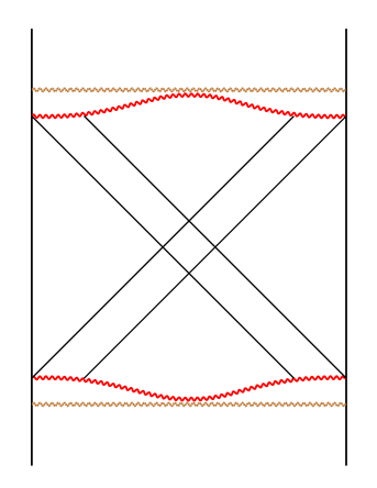
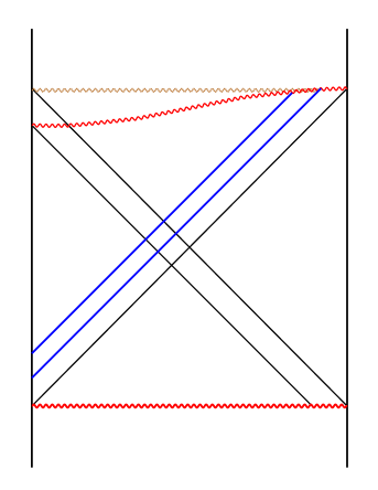
Figure 3: Penrose diagram of the Janus deformed black hole is depicted on the left. On the right, we depict the deformation of AdS₂ black hole where only $H_{l}$ is deformed in a time dependent manner.

Using the AdS/CFT dictionary developed in [21, 22], the corresponding thermofield initial state can be constructed with a Euclidean evolution

$${\cal U}_{J}=e^{-\frac{\beta}{4}H_{r}}e^{-\frac{\beta}{4}H_{l}}\,,$$ (4.7)

where $H_{l/r}$ denotes the CFT Hamitonian obtained from ${\cal L}_{L/R}$ respectively. It is straightforward to check that the vev of the operator $O_{1}$, obtained from the field theory side using the thermofield initial state and its time evolution, does indeed agree with the gravity computation in (4.4). Now by taking $\kappa_{0}=\frac{\pi}{2}$, only $H_{l}$ on the left side is deformed while the Hamiltonian on the right side remains undeformed. We introduce the reduced density matrix

$$\rho_{R}(t_{R})={\rm tr}_{L}|\Psi(t_{L},t_{R})\rangle\langle\Psi(t_{L},t_{R})|\,,$$ (4.8)

where we trace over the left-side Hilbert space. Without Janus deformation, one has $\rho_{R}(t)=\frac{1}{Z}e^{-\beta H}$, which is the usual time independent thermal density matrix. With the Janus deformation of $H_{l}$, one can view that the initial density matrix $\rho_{R}(0)$ is excited above the thermal vacuum. The deformation also makes the left-right entanglement non-maximal. This excitation is relaxed away exponentially in late time, which is basically describing thermalization of initial excitations. This explains the late time exponential decays of the vev in (4.4). The relevant time scale here is the dissipation time scale $t_{d}=\frac{\beta}{2\pi}$. Finally note that the scale $\tilde{L}$ is arbitrary. One can view that this scale is set to be there from the outset $t_{R/L}=-/+\infty$. Hence, although there is a time dependence in the vev, the system itself defined by $H_{l/r}$ is certainly time independent.

4.2 Excited black holes

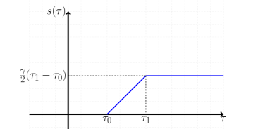
Figure 4: The source term of the operator $O_{1}$ as a function of $\tau$ is depicted. We turn on the deformation only for the left side with $s_{L}=s(\tau)$.

We would like to consider a solution that describes a change of system, beginning with a thermal state which is in equilibrium, and see its subsequent time evolution. To be definite, we shall only perturb the left side system at the moment by turning on the source term of an exactly marginal operator $O_{1}$ at some global time $\tau=\tau_{0}$. In particular we shall consider a source term given by

$$s_{L}(\tau)=\left\{\begin{array}[]{cl}0,&\ \ \ \ \ \,\tau<\tau_{0}\\ \frac{\gamma}{2}(\tau-\tau_{0}),&\ \ \ \ \ \,\tau_{0}<\tau<\tau_{1}\\ \frac{\gamma}{2}(\tau_{1}-\tau_{0}),&\ \ \ \ \ \,\tau_{1}<\tau\end{array}\right.$$ (4.10)

while $s_{R}(\tau)$ remains unperturbed in this example. We depict the functional form of the source term in Figure 4. The corresponding scalar solution reads

$$\chi=\gamma(v-v_{0})\Theta(v-v_{0})-\gamma(v-v_{1})\Theta(v-v_{1})\,,$$ (4.11)

where we introduce global null coordinates $u=\frac{1}{2}(\tau+\mu)$ and $v=\frac{1}{2}(\tau-\mu)$ and the initial/final values by $v_{0/1}=\frac{1}{2}\tau_{0/1}+\frac{\pi}{4}$. As depicted on the right side of Figure 3, only the left boundary is initially deformed, whose effect is propagating through the bulk in a causally consistent manner. The resulting bulk perturbation falls into the horizon and ends up with hitting future singularity which makes the dilaton part back-react. It never reaches the right-side boundary as dictated by the bulk causality. This is also clear from the field theory side since there is no interaction at all between the L-R systems and then no way to send any signal from one side to the other in this manner. To see the changes in the global structure of the spacetime, we turn to the description of the resulting changes in the dilaton field. We shall denote its extra contribution produced by the perturbation by $\varphi$ and thus the full dilaton field becomes

$$\phi=\bar{\phi}L\frac{\cos\tau}{\cos\mu}+\varphi\,.$$ (4.12)

Initially one has $\varphi=0$ until $v$ becomes $v_{0}$, so everything happens after $v_{0}$. For $v_{0}\leq v\leq v_{1}$, the corresponding bulk stress tensor is nonvanishing and the resulting dilaton solution reads

$$\varphi=\frac{2\pi G\gamma^{2}}{\cos\mu}\left[\,\,2(v-v_{0})\sin\mu-\cos\mu+\cos(2v_{0}-\tau)\,\,\right]\,.$$ (4.13)

For $v>v_{1}$, the bulk stress tensor vanishes and the dilaton solution becomes

$$\varphi=\frac{4\pi G\gamma^{2}}{\cos\mu}\left[\,\,(v_{1}-v_{0})\sin\mu\right.\,,$$

$$\ \ \ \left.-\sin(v_{1}-v_{0})\cos(v_{1}+v_{0})\sin\tau+\sin(v_{1}-v_{0})\sin(v_{1}+v_{0})\cos\tau\,\,\right]\,,$$ (4.14)

which takes the form of the homogeneous one in (2.10). Therefore the full solution in this region becomes the form of pure AdS₂ black hole described by

$$\phi=\phi_{BH}(\tilde{L},b,\tau_{B})$$ (4.15)

where

$${\tilde{L}}^{2} =L^{2}\Big{[}{\cal K}^{2}-g_{\gamma}^{2}(v_{1}-v_{0})^{2}\Big{]}\,,$$

$$b^{2} =\frac{{\cal K}-g_{\gamma}(v_{1}-v_{0})}{{\cal K}+g_{\gamma}(v_{1}-v_{0})}\,,$$

$$\tan\tau_{B} =-\frac{g_{\gamma}\sin(v_{1}-v_{0})\cos(v_{1}+v_{0})}{1+g_{\gamma}\sin(v_{1}-v_{0})\sin(v_{1}+v_{0})}\,.$$ (4.16)

Here, $g_{\gamma}$ is our perturbation parameter defined by $g_{\gamma}=\frac{4\pi G\gamma^{2}}{\bar{\phi}L}$ and ${\cal K}$ denotes

$${\cal K}^{2}=1+2g_{\gamma}\sin(v_{1}-v_{0})\sin(v_{1}+v_{0})+g_{\gamma}^{2}\sin^{2}(v_{1}-v_{0})\,.$$ (4.17)

One finds $\tilde{L}\geq L$ at least to the leading order in $g_{\gamma}$ where we used the fact $0\leq v_{0},v_{1}\leq\frac{\pi}{2}$. Hence the Beckenstein-Hawking temperature of the resulting black hole increases after the perturbation. Though the scalar perturbation parameter $\gamma$ can take either signs, the dilaton perturbation parameter $g_{0}$ is always non-negative definite. Thus the change in temperature ought to be independent of the signatures of the scalar perturbation parameter $\gamma$. This perhaps reflects the fact the dual field theory side has to be strongly coupled to have a gravity description. In the gravity side, the black hole solution is independent of turning on a constant moduli parameter described by the constant part of the scalar field. This is consistent with the fact that our dilaton gravity description corresponds to the strong coupling limit of the boundary quantum system. We shall not explore any further details of the above aspect in this note, since we are more concerned in the other aspects such as teleportation.

One finds $b\neq 1$ due to the perturbation and the shift parameter of the singularity is nonvanishing only in the left side. It can be identified as

$$\Delta\tau_{L}=\tau_{B}-\arcsin\frac{g_{\gamma}(v_{1}-v_{0})}{{\cal K}}\,,$$ (4.18)

which is certainly negative definite as expected. Thus we conclude that one cannot send a signal from one side to the other using the above perturbation since the L-R sides are causally disconnected with each other. This is quite consistent with the field theory side since no interaction between the left and the right boundaries is turned on. We depict the resulting global structure on the right of Figure 3.

Finally one may consider more general form of perturbation where the scalar solution takes the form

$$\chi=\chi_{L}=\sum^{n_{L}}_{i=0}\gamma^{L}_{i}\,(v-v_{i})\Theta(v-v_{i})\,,$$ (4.19)

where $\sum_{i}\gamma_{i}^{L}=0$ and we order $v_{i}$ such that $v_{i+1}>v_{i}$. Of course one may consider the perturbation

$$\chi=\chi_{R}=\sum^{n_{L}}_{i=0}\gamma^{R}_{i}\,(u-u_{i})\Theta(u-u_{i})\,,$$ (4.20)

where again $\sum_{i}\gamma_{i}^{R}=0$ and we order $u_{i}$ such that $u_{i+1}>u_{i}$. This is describing the perturbation where the signal is sent from the right boundary. The only changes is we flip the L-R sides by the transformation $\mu\leftrightarrow-\mu$. The corresponding dilaton perturbations can be identified straightforwardly for the both types. When the both perturbations are present, interestingly one can get the corresponding solution by a simple linear superposition

$$\chi=\chi_{L}+\chi_{R}\,,$$

$$\varphi=\varphi_{L}+\varphi_{R}\,,$$ (4.21)

where $\varphi_{L/R}$ is denoting the dilaton solution with the scalar field $\chi_{L/R}$ respectively. Thus the solutions in the above describe rather general perturbations of the black hole system. We shall use these constructions to describe teleportees in later sections.

5 Double trace deformation and stress tensor

In this section we consider the back-reaction in the dialton field by the 1-loop stress tensor of the bulk scalar field $\chi$ with the boundary condition which is related to the double trace deformation of the boundary theory. The bulk free scalar field $\chi$ in AdS space can have the asymptotic behavior $r^{-\Delta_{\pm}}$ along the radial direction $r$ where the fall-off power $\Delta_{\pm}$ is given by (3.2). When $-1/4<m^{2}<0$, both modes of the power $\Delta_{\pm}$ become normalizable and their duals may be realized as unitary scalar operators. In particular $\Delta_{-}$ is ranged over $(0,\frac{1}{2})$, which allows us to consider the double trace deformation in the dual boundary theory [24, 25, 26]. In the following we set $\Delta\equiv\Delta_{-}$ and then $\Delta_{+}=d-\Delta$. In this case, one may consider a general mixed boundary condition such that the boundary values of two modes become proportional.

In our context for the coupling between the left and right boundary operators, the asymptotic behavior of the scalar field in the right/left wedges in the Penrose diagram is given by

$$\chi(t,r)|_{R/L}=\frac{\alpha_{R/L}}{r^{\Delta}}+\cdots+\frac{\beta_{R/L}}{r^{1-\Delta}}+\cdots\,,$$ (5.1)

and the mixed boundary condition corresponds to

$$\beta_{L}(t)=h(-t)\alpha_{R}(-t)\,,\qquad\beta_{R}(t)=h(t)\alpha_{L}(-t)\,.$$ (5.2)

According to the AdS/CFT correspondence for the double trace deformation [25], this solution corresponds to the deformation of the Hamiltonian in the boundary theory given by

$$\delta H(t)=-h(t){\cal O}_{R}(t){\cal O}_{L}(-t)\,,$$ (5.3)

where $\mathcal{O}_{R,L}$ are scalar operators of dimension $\Delta$ dual to $\chi$. This is a relavant deformation of dimension $2\Delta$ and the coupling $h(t)$ has dimension $1-2\Delta$.

Now suppose that $h(t)=0$ when $t<t_{0}$ so that we turn on the deformation at $t=t_{0}$. Then, as in the BTZ case [27, 7], the leading correction to the bulk 2-point function is expressed in the interaction picture as

$$G \equiv F(t,t^{\prime})+F(t^{\prime},t)$$

$$=i\int^{t}_{t_{0}}d\tilde{t}\left\langle[\delta H(\tilde{t}),\chi_{R}(t)],\chi_{R}(t^{\prime})\right\rangle+i\int^{t^{\prime}}_{t_{0}}d\tilde{t}\left\langle\chi_{R}(t)[\delta H(\tilde{t}),\chi_{R}(t^{\prime})]\right\rangle\,,$$ (5.4)

where the coordinate $r$ is suppressed for simplicity. Here we are interested in the violet-colored right wedge in Figure 5 which is the intersection of the spacelike region of the point $t_{L}=-t_{0}$ at the left boundary and the timelike region of the point $t=t_{R}=t_{0}$ at the right boundary. In particular, we are not interested in the green-colored region deep inside the horizon which is timelike from both boundary points at $t_{R/L}=\pm t_{0}$. Then we can calculate $F(t,t^{\prime})$ in the large $N$ limit by noting that $\mathcal{O}_{L}$ commutes with $\chi_{R}$ due to causality,

$$F(t,t^{\prime})\simeq-i\int_{t_{0}}^{t}d\tilde{t}h(\tilde{t})\langle\chi_{R}(t^{\prime})\mathcal{O}_{L}(-\tilde{t})\rangle\langle[\mathcal{O}_{R}(\tilde{t}),\chi_{R}(t)]\rangle\,.$$ (5.5)

The first correlation function containing $\mathcal{O}_{L}$ may be expressed in terms of the bulk-boundary propagator (B.1) in the appendix by use of the KMS condition [28, 29, 30, 15]

$$\langle\mathcal{O}_{R}(t)\mathcal{O}_{L}(t^{\prime})\rangle_{\textrm{tfd}}=\langle\mathcal{O}_{R}(t)\mathcal{O}_{R}(t^{\prime}+i\beta/2)\rangle_{\textrm{tfd}}\,,$$ (5.6)

and the second factor yields the retarded function (B). Thus,

$$F(t,t^{\prime})=2\sin\pi\Delta\int_{t_{0}}^{t}d\tilde{t}h(\tilde{t})K_{\Delta}(t^{\prime}+\tilde{t}-i\beta/2)K_{\Delta}^{r}(t-\tilde{t})\,.$$ (5.7)

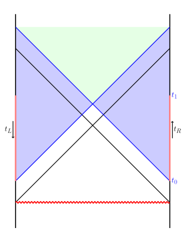
Figure 5: The deformation $\delta H(t)$ is turned on at $t_{R/L}=\pm t_{0}$ and turned off at $t_{R/L}=\pm t_{1}$. The violet-colored right wedge is the intersection of the spacelike region of the point $t_{L}=-t_{0}$ at the left boundary and the timelike region of the point $t_{R}=t_{0}$ at the right boundary.

The 1-loop stress tensor can be computed through the bulk 2-point function $G(x,x^{\prime})$ as

$$T_{ab}=\lim_{x^{\prime}\rightarrow x}\Big{[}\partial_{a}\partial^{\prime}_{b}G(x,x^{\prime})-\frac{1}{2}g_{ab}g^{\rho\sigma}\partial_{\rho}\partial^{\prime}_{\sigma}G(x,x^{\prime})-\frac{1}{2}g_{ab}m^{2}G(x,x^{\prime})\Big{]}\,,$$ (5.8)

where we have to subtract the singular expressions in the coincident limit. As in the BTZ case [7], the zeroth order term in $h$ gives a vanishing contribution to $\int dUT_{UU}$ on the horizon $V=0$. A nonvanishing result is obtained with the first order correction (5). In the following, we assume that $h(t)$ is a nonvanishing constant only in the interval $[t_{0},t_{1}]$,

$$h(t)=\begin{cases}h(\frac{2\pi}{\beta})^{1-2\Delta},&\quad t_{0}\leq t\leq t_{1},\\ 0,&\quad\text{otherwise}~{}~{}\,,\end{cases}$$ (5.9)

where $h$ is constant. In Kruskal coordinates, we find

$$T_{UU}(U,V)=2\lim_{U^{\prime},V^{\prime}\rightarrow U,V}\partial_{U^{\prime}}\partial_{U}F(U,U^{\prime})\,,$$ (5.10)

where $F(U,U^{\prime})$ is given by

$$F(U,U^{\prime})=hN_{\Delta}\int^{U_{f}}_{U_{0}}\frac{d{\cal S}}{{\cal S}}\left[\frac{1+U^{\prime}V^{\prime}}{U^{\prime}{\cal S}-V/{\cal S}+1-U^{\prime}V^{\prime}}\right]^{\Delta}\left[\frac{1+UV}{U/{\cal S}-V{\cal S}-(1-UV)}\right]^{\Delta}\,,$$ (5.11)

with

$$N_{\Delta}\equiv\frac{1}{2\pi}~{}\frac{2^{2\Delta-2}\Gamma^{3}(\Delta)}{\Gamma^{2}(2\Delta)\Gamma(1-\Delta)}\,,\qquad\qquad U_{f}\equiv\left\{\begin{array}[]{ll}U\,,&\quad\quad U_{0}\leq U<U_{1},\\ U_{1}\,,&\quad\quad~{}~{}~{}~{}U\geq U_{1}~{}~{}~{}\,.\end{array}\right.$$ (5.12)

6 Traversable wormholes

In this section we compute the back-reacted deformation of the dilaton field through the 1-loop stress tensor by the coupling between the left and right boundary operators. We will follow closely the steps in Ref. [7] while some aspects could be addressed more concretely. One can see the reduction of the horizon radius and the uplift of the position of the singularity compared before the deformation. As a result, one can check that the thermodynamic 1st law holds in our setup, in addtion that wormholes become traversable. Some formulae are relegated to Appendices for readability.

On the initial condition of infalling matters such that $T_{UV}(U,V)=0$ for any value in the range of $U\leq U_{0}$, the solution to (2) of dilaton field $\phi$, sourced by the stress tensor $T_{ab}$, can be shown to become (see Appendix A)

$$\phi = \bar{\phi}L\frac{\cos\tau}{\cos\mu}+\varphi\,,$$

$$\varphi = -\frac{1}{1+UV}\int^{U}_{U_{0}}dP~{}(U-P)(1+PV)T_{UU}(P,V)\,.$$ (6.1)

Note that, in terms of the global null coordinates with the change of a variable $P=\tan p$, the dilaton field solution could also be written as

$$\varphi(u,v)=\frac{1}{\cos(u-v)}\int^{u}_{u_{0}}dp~{}\sin(p-u)\cos(p-v)~{}T_{uu}(p,v)\,.$$ (6.2)

By inserting the expression of $T_{UU}$ in (5.10) to (6), one can show, after some calculation, that the deformation of the dilation field $\phi$ is given by (see Appendix B)

$$\varphi(U,V)=2h\Delta N_{\Delta}\int^{U_{f}}_{U_{0}}d{\cal S}\frac{{\cal S}^{2\Delta-1}}{(1+{\cal S}^{2})^{2\Delta}}\Big{[}w^{1-\Delta}(1-w)^{2\Delta-1}+\Delta\frac{1+w}{1-w}B_{w}(1-\Delta,2\Delta)\Big{]}\,,$$ (6.3)

where $w$ is defined by

$$w\equiv\frac{({\cal S}-V)(U-{\cal S})}{(1+{\cal S}V)(1+{\cal S}U)}\,,$$

and $U_{f}$ is defined in Eq. (5.12). Through the change of a variable $\tan s\equiv\frac{1}{2}({\cal S}-1/{\cal S})$, the above solution can also be written as

$$\varphi(u,v)=\frac{h\Delta N_{\Delta}}{2^{2\Delta-1}}\int^{s_{f}}_{s_{0}}ds\,(\cos s)^{2\Delta-1}\Big{[}w^{1-\Delta}(1-w)^{2\Delta-1}+\Delta\frac{1+w}{1-w}B_{w}(1-\Delta,2\Delta)\Big{]}\,,$$ (6.4)

where $w$ and $s_{f/0/1}$ are given by

$$w=\frac{\sin(u+v-s)-\cos(u-v)}{\sin(u+v-s)+\cos(u-v)}\,,\quad\tan s_{f}=\frac{1}{2}(U_{f}-\frac{1}{U_{f}})\,,\quad\tan s_{0/1}=\frac{1}{2}(U_{0/1}-\frac{1}{U_{0/1}})\,.$$

Now, let us consider the near boundary region $\mu\simeq\pi/2$ after turning off the L-R coupling $h$, at which the singularity meets the right boundary of AdS₂. Note that this limit corresponds to $w=1$ in the incomplete Beta function $B_{w}(a,b)$. By using the expansion of $B_{w}(a,b)$ around $w=1$, the deformed dilaton field in the above limit becomes

$$\varphi(\tau,\mu)=\frac{8\pi G}{\cos\mu}\Big{[}h\alpha_{s}\sin\tau+h\alpha_{c}\cos\tau\Big{]}+O(\cos^{2\Delta}\mu)\,,$$ (6.5)

where $\alpha_{s}$ and $\alpha_{c}$ are given by

$$\alpha_{s} =2\Delta^{2}N_{\Delta}B(1-\Delta,2\Delta)~{}\left[B_{z_{0}}(\Delta+\frac{1}{2},\Delta+\frac{1}{2})-B_{z_{1}}(\Delta+\frac{1}{2},\Delta+\frac{1}{2})\right]\,,$$

$$\alpha_{c} =-\Delta N_{\Delta}B(1-\Delta,2\Delta)~{}\Big{[}z_{0}^{\Delta}(1-z_{0})^{\Delta}-z_{1}^{\Delta}(1-z_{1})^{\Delta}\Big{]}\,,\quad\quad z_{i}\equiv\frac{1}{1+U^{2}_{i}}\,.\qquad$$ (6.6)

Combined with the homogeneous part of the solution, the full solution becomes

$$\phi(\tau,\mu)=\bar{\phi}L\frac{\cos\tau}{\cos\mu}+\frac{8\pi G}{\cos\mu}\Big{[}h\alpha_{s}\sin\tau+h\alpha_{c}\cos\tau\Big{]}+O(\cos^{2\Delta}\mu)\,.$$ (6.7)

We would like to understand the deformation of this geometry and the structure of the singularity in the asymptotic region of our interest. We compare this with the general form of the static black hole solution

$$\phi=\phi_{BH}(L+\delta L,1+\delta b,\delta\tau_{B})\,,$$ (6.8)

where $\delta L$, $\delta b$ and $\delta\tau_{B}$ are describing deformation of the black hole due to the L-R coupling. This leads to the identification of parameters

$$\left(1+\frac{\delta L}{L}\right)^{2} =\left(1+\frac{8\pi G}{\bar{\phi}L}h\alpha_{c}\right)^{2}+\left(\frac{8\pi G}{\bar{\phi}L}h\alpha_{s}\right)^{2}\,,$$

$$\delta\tau_{B} =\arctan\frac{\frac{8\pi G}{\bar{\phi}L}h\alpha_{s}}{1+\frac{8\pi G}{\bar{\phi}L}h\alpha_{c}}\,,$$

$$\delta b =0\,.$$ (6.9)

These parameters could also be read from (B.44) and (C.2) in Kruskal coordinates directly which we have done to the linear order in $Gh$. Since the static black hole is characterized by the temperature only as we discussed in section 2, one relevant physical parameter is $\delta L$ that is related to the temperature $T+\delta T$ with $\delta T=\frac{1}{2\pi}\frac{\delta L}{\ell^{2}}$. The other relevant physical parameter is the shift of singularity identified as

$$\Delta\tau^{R}_{+}=\delta\tau_{B}\sim\frac{8\pi G}{\bar{\phi}L}h\alpha_{s}+O(G^{2}h^{2})\,.$$ (6.10)

This expression may take either signs. We shall choose $h$ positive where the shift becomes positive-definite. It then tells us that the wormhole becomes traversable since the position of the singularity is uplifted in the right wedge as can be seen from Figure 6 by the amount $\Delta\tau^{R}_{+}$. Since our configuration is left-right symmetric under the exchange of $\mu\leftrightarrow-\mu$, one has $\Delta\tau^{R}_{+}=\Delta\tau^{L}_{+}$ both of which are denoted as $\Delta\tau$ in Figure 6. Note also that the expression of $\alpha_{s}$ is effectively identical to the expression of the averaged null energy condition violation $\int^{\infty}_{U_{0}}dU\,T_{UU}$. In this manner, one can send a signal from one side to the other through the wormhole now.

Figure 6: Penrose diagram of the traversable wormhole is depicted in this figure. The left-right boundaries are now causally connected as the wormhole becomes traversable. The shape of the upper singularity is not precise as it is curved in general.

This wormhole parameter is monotonically increasing as a function of $z_{0}\in[0,1]$. This implies that the earlier the L-R interaction starts, the bigger the traversable gap opens up, which is in accordance with our physical intuition. Its maximum is attained at $z_{0}/z_{1}=1/0$ corresponding to $U_{0}/U_{1}=0/\infty$ or $t_{0}/t_{1}=-/+\infty$.

In our two-dimensional model of black holes, the energy $E_{R}$ could be identified with the black hole mass $M$, and the black hole entropy change can be read from the change of horizon area as

$$\delta S_{BH}=\frac{\bar{\phi}}{4G}\delta L={\cal C}\delta T\,$$ (6.11)

to the leading order in $Gh$ taking the small variation limit. Note that, once $t_{0}\geq 0$, the horizon radius is reduced by the amount $\delta L=\frac{8\pi G}{\bar{\phi}L}\alpha_{c}<0$ and the Beckenstein-Hawking temperature will be reduced accordingly as well. This reduction of the horizon radius is consistent with the entropy reduction in the measurement process during the quantum teleportation, which is argued to be dual to the traversable wormhole.

To see the consistency of this change of the horizon radius, let us return to the energy change by the deformed Hamiltonian in the boundary theory. Using expression for the black hole energy (or mass) in (2.31), the change in energy is identified as

$$\delta E={\cal C}T\delta T=\frac{L}{\ell^{2}}h\alpha_{c}\,.$$ (6.12)

In fact this expression can be confirmed directly from the boundary computation as follows. Note that, along the method in the Ref. [7], the change of energy by the Hamiltonian deformation is given by

$$\delta E_{R} =-i\int^{t_{1}}_{t_{0}}dt^{\prime}\langle\Psi(t^{\prime})|[\delta H(t^{\prime}),H_{R}]|\Psi(t^{\prime})\rangle$$

$$=\int^{t_{1}}_{t_{0}}dt^{\prime}h(t^{\prime})\langle\Psi(t^{\prime})|\dot{\cal O}_{R}{\cal O}_{L}(t^{\prime})|\Psi(t^{\prime})\rangle$$

$$=h\Big{(}\frac{2\pi}{\beta}\Big{)}^{1-2\Delta}\int^{t_{1}}_{t_{0}}dt^{\prime}~{}\frac{1}{2}\partial_{t^{\prime}}\Big{[}\lim_{r^{\prime}\rightarrow\infty}\Big{(}\frac{r^{\prime}}{\ell^{2}}\Big{)}^{\Delta}K_{\Delta}(2t^{\prime}-\frac{i}{2}\beta)\Big{]}$$

$$=h\Big{(}\frac{L}{\ell^{2}}\Big{)}\frac{\Gamma^{2}(\Delta)}{8\pi\Gamma(2\Delta)}\Big{[}\frac{1}{(\cosh\frac{Lt_{1}}{\ell^{2}})^{2\Delta}}-\frac{1}{(\cosh\frac{Lt_{0}}{\ell^{2}})^{2\Delta}}\Big{]}\,,$$ (6.13)

where we use the undeformed thermofield initial state defined in (2.34) with ${\cal U}={\cal U}_{0}$. Further noting $U_{i}=e^{Lt_{i}/\ell^{2}}$ in the right boundary, it is then obvious that the first law holds in our limit

$$\delta E_{R}=\delta M=T\delta S\,.$$ (6.14)

We find that $\delta E_{R}$ or $\delta S$ becomes positive if $0\geq t_{1}>t_{0}$ but the wormhole is still traversable. This behavior is related to thermalization of perturbation as suggested by the time dependence in (6) shows exponential decaying behaviours with the dissipation time scale given by $t_{d}=\frac{\beta}{2\pi}$. This earlier perturbation still makes wormhole traversable while the perturbation is allowed to be thermalized enough to have an increased total entropy of the system. Of course by the first law, the corresponding change of energy should be positive. The overall picture here is nothing new. We just make its bulk description direct and quantitative.

Finally one may show that, to the leading in $h$, our traversable wormhole solution in this section is indeed consistent with that from the boundary reparametrization dynamics in [8, 10]. See Appendix E for the detailed comparison.

7 Full bulk teleportation

In this section, we shall present a simple teleportation model in the boundary side and various bulk solutions which include a traversable wormhole and a teleportee state traveling through the wormhole from the left to the right boundaries.

Teleportation is sending a quantum state to a remote place via EPR entanglement channel. Let us give its elementary introduction here. Alice on the left side would like to teleport a qubit

$$|T\rangle=c_{0}|0\rangle_{T}+c_{1}|1\rangle_{T}\,,$$ (7.1)

from the left to the right boundaries. We model the L-R entanglement by an EPR pair

$$|\Psi\rangle_{LR}=\frac{1}{\sqrt{2}}\sum^{1}_{i=0}|i\rangle_{L}|i\rangle_{R}\,,$$ (7.2)

where $i,j,k,\theta_{1},\theta_{2}=0,1$. This $|T\rangle$ is added to the left side at some point. One then represents the left side system in a new basis spanned by

$$|\theta_{1}\theta_{2}\rangle_{M}=\frac{1}{\sqrt{2}}\left[\,|\theta_{1}0\rangle_{TL}+(-)^{\theta_{2}}|1-\theta_{1}~{}~{}1\rangle_{TL}\right]\,,$$ (7.3)

each of which is maximally entangled. With this new basis, the full system can be represented by

$$|T\rangle|\Psi\rangle_{LR}=\frac{1}{2}\sum_{\theta_{1},\theta_{2},i,k}|\theta_{1}\theta_{2}\rangle_{M}(U^{-1}_{\{\theta_{1}\theta_{2}\}})_{ik}c_{k}|i\rangle_{R}\,,$$ (7.4)

where $U_{\{\theta_{1}\theta_{2}\}}=\sigma^{\theta_{1}}_{1}\sigma^{\theta_{2}}_{3}$ with $\sigma_{1,2,3}$ denoting the standard Pauli matrices. Now Alice makes a measurement in the $M$ basis ending up with a particular state $|\theta_{1}\theta_{2}\rangle_{M}$ and sends its result $\{\theta_{1},\theta_{2}\}$ to Bob on the right side via an extra classical channel. This classical channel is completely independent of our bulk. At this stage the total state becomes

$$\sum_{i,k}|\theta_{1}\theta_{2}\rangle_{M}(U^{-1}_{\{\theta_{1}\theta_{2}\}})_{ik}c_{k}|i\rangle_{R}\,.$$ (7.5)

Once Bob gets the message, he performs a unitary transform of his state by the action $V_{\theta}=U_{\{\theta_{1}\theta_{2}\}}$ and then the resulting state becomes

$$|\theta_{1}\theta_{2}\rangle_{M}\sum_{k}c_{k}|k\rangle_{R}\,.$$ (7.6)

This completes the quantum teleportation of $|T\rangle$ from the left to the right. Of course one can consider more general setup where one has an L-R entanglement involving many qubits and teleports more than one qubit. In particular when one uses our Einstein-Rosen bridge as the L-R entanglement based on the so called ER=EPR relation [31], there will be in general a thermailzation of $|T\rangle$ state after its inclusion to the left side. Measurement can be made by picking up an arbitrary qubit of $L$ system and forming a maximally entangled basis where we assume $|T\rangle$ is one qubit. After the measurement, Alice again sends the result of measurement to Bob. Bob then recovers the $|T\rangle$ by the action of an appropriate unitary transformation. For more detailed discussions, we refer to Ref. [9].

A few comments are in order. First of all, the measurement in general makes the L-R entanglement reduced and the L-T system entangled instead. The second essential feature is the L-R coupling by the measurement $M^{\theta}_{L}$ on the left side and the recovery action $V^{\theta}_{R}$ on the right side. This coupling basically makes the wormhole traversable as we verified in the previous section.

We now turn to our bulk description. We shall basically combine the traversable wormhole in (6.3) and the bulk-traveling solution (4.12). As was done in Ref. [8], we would like to suppress any higher loop corrections in our computation. For this purpose, we shall introduce $K_{\theta}$ dimension $\Delta$ and $K_{T}$ dimension one operators respectively for the L-R coupling of the traversable wormhole and the teleportee degrees and excite them altogether coherently. We shall fix parameters ${\bar{\gamma}}^{2}$ and $\bar{h}$ which are defined by

$${\bar{\gamma}}^{2} =\frac{4\pi G}{\bar{\phi}L}K_{T}\gamma^{2}\,,$$

$${\bar{h}}\ =\frac{8\pi G}{\bar{\phi}L}K_{\theta}h\,,$$ (7.7)

while taking large $K_{T,\theta}$ limit. This then makes any possible higher loop corrections suppressed. The combined solutions can be presented in the form

$$\phi=\frac{\bar{\phi}L}{\cos\mu}\left[\,Q_{\mu}\sin\mu+Q_{s}\sin\tau+(1+Q_{c})\cos\tau\,\right]+O(\cos^{2\Delta}\mu)\,,$$ (7.8)

in near right-boundary region where the L-R coupling and boundary interactions are not present or were already turned off. The wormhole opening parameter of the right boundary is given by

$$\Delta\tau^{+}_{R}=\arctan\frac{Q_{s}}{1+Q_{c}}$$ (7.9)

and the traversability condition of the resulting wormhole requires $Q_{s}>0$ which leads to positive $\Delta\tau^{+}_{R}$. Let us begin with a minimal one.

Solution $A$ : For $v_{0}>v\geq 0$ and $u\geq\frac{1}{2}\left(s_{1}+\frac{\pi}{2}\right)$, one has

$$Q_{s}=\bar{h}\alpha_{s}\,,\qquad Q_{c}=\bar{h}\alpha_{c}\,,$$ (7.10)

with $Q_{\mu}=0$. On the other hand, for $v\geq v_{1}$ and $u\geq\frac{1}{2}\left(s_{1}+\frac{\pi}{2}\right)$,

$$Q_{\mu}={\bar{\gamma}}^{2}(v_{1}-v_{0})\,,$$

$$Q_{s}=\bar{h}\alpha_{s}-{\bar{\gamma}}^{2}\sin(v_{1}-v_{0})\cos(v_{1}+v_{0})\,,$$

$$Q_{c}=\bar{h}\alpha_{c}+{\bar{\gamma}}^{2}\sin(v_{1}-v_{0})\sin(v_{1}+v_{0})\,.$$ (7.11)

Since $\bar{h}\alpha_{s}$ is positive definite with our choice $h>0$, the wormhole becomes traversable. Then one may send a signal from the left to the right while the wormhole is traversable. Therefore the $|T\rangle$ state added to the left side will appear on the right side which is the teleportation from the left to the right boundaries. One finds that the wormhole opening parameter $\Delta\tau^{+}_{R}$ is dependent in general on the degrees and details of the teleportee. We would like to take $v_{1}\leq\frac{\Delta\tau^{+}_{R}}{2}$ such that no information is lost into the singularity behind the horizon. Since the added contribution to $Q_{c}$ by the teleportee is given by

$${\bar{\gamma}}^{2}\sin(v_{1}-v_{0})\sin(v_{1}+v_{0})\,.$$ (7.12)

which is always positive definite. Then there is a corresponding increase of the black hole entropy and mass, which may be used as a criterion about how many qubits are transported.

Let us now turn to the case where Bob also throws a matter into the horizon from the right. In our case, this matter wave is again described by the massless scalar field introduced in Section 4.2. Namely, we consider the left-moving wave

$$\chi_{R}=\gamma_{R}(u-u_{0})\Theta(u-u_{0})-\gamma_{R}(u-u_{1})\Theta(u-u_{1})$$ (7.13)

in addition to the L-R coupling and the teleportee of Solution A. Here of course we take $u_{1}\geq u_{0}$ with $u_{i}\in[0,\frac{\pi}{2}]$. The resulting full system is described by the following.

Solution B: For the region $v_{0}\geq v\geq 0$ and $u\geq{\rm max}\left(u_{1},\frac{1}{2}\left(s_{1}+\frac{\pi}{2}\right)\right)$, the dilaton is described by

$$Q_{\mu}=-{\bar{\gamma}_{R}}^{2}(u_{1}-u_{0})\,,$$

$$Q_{s}=\bar{h}\alpha_{s}-{\bar{\gamma}}_{R}^{2}\sin(u_{1}-u_{0})\cos(u_{1}+u_{0})\,,$$

$$Q_{c}=\bar{h}\alpha_{c}+{\bar{\gamma}}_{R}^{2}\sin(u_{1}-u_{0})\sin(u_{1}+u_{0})\,.$$ (7.14)

For the region $v\geq v_{1}$ and $u\geq{\rm max}\left(u_{1},\frac{1}{2}\left(s_{1}+\frac{\pi}{2}\right)\right)$, the dilaton parameters are given by

$$Q_{\mu}={\bar{\gamma}}^{2}(v_{1}-v_{0})-{\bar{\gamma}_{R}}^{2}(u_{1}-u_{0})\,,$$

$$Q_{s}=\bar{h}\alpha_{s}-{\bar{\gamma}}^{2}\sin(v_{1}-v_{0})\cos(v_{1}+v_{0})-{\bar{\gamma}}_{R}^{2}\sin(u_{1}-u_{0})\cos(u_{1}+u_{0})\,,$$

$$Q_{c}=\bar{h}\alpha_{c}+{\bar{\gamma}}^{2}\sin(v_{1}-v_{0})\sin(v_{1}+v_{0})+{\bar{\gamma}}_{R}^{2}\sin(u_{1}-u_{0})\sin(u_{1}+u_{0})\,.$$ (7.15)

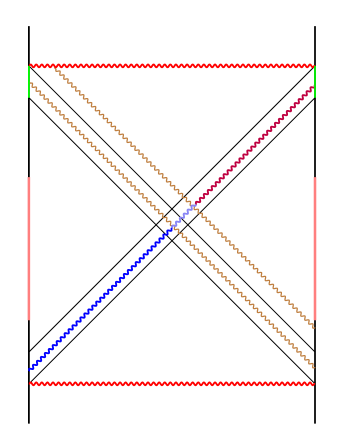
Figure 7: The full bulk teleportation with additional matters thrown into the horizon from the right side. The teleportee will be affected by this bulk encounter. Again the shape of the upper singularity is not precise as it may be curved in general.

When the perturbation from the right side is too strong such that

$${\bar{\gamma}}_{R}^{2}\sin(u_{1}-u_{0})\cos(u_{1}+u_{0})\geq\bar{h}\alpha_{s}\,,$$ (7.16)

the wormhole is no longer traversable since $\Delta\tau^{+}_{R}$ of the solution in (7) becomes non positive. Of course, one has then a usual two-sided black hole system where any perturbations thrown into horizon hit the future singularity inevitably. If the extra matter thrown into the black hole from the right side is not too big such that the condition (7.16) is violated, the wormhole remains traversable and the teleportee can be sent from the left to the right sides through the wormhole. It is clear that the teleportee will meet the matter from the right side while transported. It can record and report this encounter to Bob on the right side. Hence one may conclude that the bulk wormhole is experimentally observable, which was emphasized in Ref. [9].

As was mentioned in the introduction, in this note we have ignored any possible back-reaction effect caused by the bulk excitations. Once there are any excitations, identification of the time coordinate $t_{L/R}$ of the boundary system as a function of the bulk time coordinate $t$ becomes nontrivial. Without any excitations, one has an identification $t(t_{L/R})=t_{L/R}$ for the AdS black holes of Section 2. With excitations, the reparametrization dynamics $t(t_{L/R})$ can be nontrivial, which is one of the main points of Refs. [11, 8]. Indeed the presence of the bulk teleportee will make the $t(t_{L/R})$ dynamically nontrivial. Hence this back-reaction effect has to be taken into account. In order to fix the action of the L-R interactions in the presence of this back-reaction effect, one then has to modify the L-R coupling strength $h$ in an appropriate manner. For a given L-R interaction specified by the boundary time $t_{L/R}$, one may ask if there is a limit in the number of qubits that can be teleported [8]. In our formulation, we are not able to show this limit which requires the identification of $t(t_{L/R})$.

Alternatively one may ask the following to see the above limitation in our formulation. Namely one may effectively makes $\bar{h}$ together with the number of qubits of the teleportee state small enough such that the above back-reaction effect is negligible. In this situation, one might be able to see the above limitation. For this, we take $\bar{h}\ll 1$. Then clearly $\Delta\tau^{R}_{+}$ is of $O(\bar{h})$. Then $v_{0},v_{1}\sim O(\bar{h})$ since $v_{1}\leq\frac{1}{2}\Delta\tau^{R}_{+}$. The resulting change in the entropy due to the presence of the teleportee will be of $O(\bar{\gamma}^{2}{\bar{h}}^{2})$ since

$$\Delta S\propto{\bar{\gamma}}^{2}\sin(v_{1}-v_{0})\sin(v_{1}+v_{0})\sim O(\bar{\gamma}^{2}{\bar{h}}^{2})\,.$$ (7.17)

Since Solution A has the dependence on the parameter ${\bar{\gamma}}^{2}(v_{1}-v_{0})$, which we would like to keep as small as $O(\bar{h})$ to control the approximation. (The entropy change is the order of the back-reaction effect $O({\bar{h}}^{2})$ which we have ignored in our approximation.) At any rate, the teleported bits are too small and it is not possible to see any limitation in this manner. Further study in this direction is required.

8 Conclusions

In this note, we have described a complete bulk picture of the quantum teleportation through a traversable wormhole in the two-dimensional dilaton gravity with a scalar field. First, we have constructed various full back-reacted solutions describing perturbation of a black hole and its thermalization. To realize a teleportee state, we have considered a specific time-dependent Janus deformation of AdS₂ black hole where only the left boundary is initially deformed but the effect is propagating through the bulk obeying the causality. This solution by itself cannot be used to send signal from one boundary to the other because the dilaton back reacts in the way that the signal hits the future singularity before reaching the other side of the boundary. This is consistent with the field theory side since L-R systems are completely decoupled from each other and hence there is no way to send any signal from one side to the other.

The situation, however, changes if we turn on the double trace interaction between two boundaries which violates the average null-energy condition in the bulk. It renders the wormhole traversable and, to the leading order, the traversability can be maintained in the presence of the teleportee state. We have solved of the equation of motion for the dilaton for a general stress tensor. It allows us to identify the relevant parameters which are responsible for the transversability and the change of the horizon area. The entropy is changed consistently with the black hole first law. Our solutions have then further be extended to include extra matter thrown into the the black hole from the boundary that the teleportee would reach. The teleportee would meet the matter during transportation, which shows that the bulk wormhole is experimentally observable.

In this note, we have not attempted to include any possible back reactions in identification of the boundary time coordinates $t_{L/R}$ as a function of the bulk time coordinate $t$. Though our bulk solutions are fully consistent in their own right, we need a precise identification of $t(t_{L/R})$ in order to have their proper boundary interpretation. Indeed it is clear that the naive identification $t(t_{L/R})=t_{L/R}$ for the AdS black hole should be modified in the presence of the bulk teleportee and other bulk interactions. This would require the formulation of Ref. [11] and further study is needed in this direction.

Appendix A Coordinates and dilaton solution

In this appendix, we would like to solve the equation of motion (2) in the presence of the energy-momentum tensor $T_{ab}$. In the Kruskal coordinates of AdS₂, the metric is given by

$$ds^{2}=-\frac{4\ell^{2}dUdV}{(1+UV)^{2}}\,.$$ (A.1)

The Kruskal and global coordiantes for AdS₂ are related by

$$U=\tan\frac{\tau+\mu}{2}\,,\qquad V=\tan\frac{\tau-\mu}{2}\,,$$ (A.2)

and in the Kruskal coordinates, (2) becomes

$$\frac{1}{(1+UV)^{2}}\partial_{U}\left[(1+UV)^{2}\partial_{U}\phi\right] =-8\pi GT_{UU}$$

$$\frac{1}{(1+UV)^{2}}\partial_{V}\left[(1+UV)^{2}\partial_{V}\phi\right] =-8\pi GT_{VV}$$

$$-\partial_{U}\partial_{V}\phi-\frac{2}{(1+UV)^{2}}\phi =-8\pi GT_{UV}$$ (A.3)

where the energy-momentum tensor $T_{ab}$ satisfies the conservation $\nabla^{a}T_{ab}=0$. Explicitly,

$$(1+UV)^{2}\partial_{V}T_{UU}+\partial_{U}\left[(1+UV)^{2}T_{UV}\right] =0\,,$$

$$(1+UV)^{2}\partial_{U}T_{VV}+\partial_{V}\left[(1+UV)^{2}T_{UV}\right] =0\,.$$ (A.4)

(A) can readily be integrated to obtain the general solution of $\phi(U,V)$. In the following we will set $8\pi G=1$. Due to the conservation equation (A), there are several different ways to express the solution. One way is to express it in a symmetric way with respect to $U$ and $V$,

$$\phi(U,V)=-\frac{1}{1+UV} \left[\int_{U_{0}}^{U}(U-t)(1+tV)T_{UU}(t,V_{0})\,dt+\int_{V_{0}}^{V}(V-s)(1+sU)T_{VV}(U_{0},s)\,ds\right.~{}~{}~{}$$

$$\left.-\int_{V_{0}}^{V}\int_{U_{0}}^{U}\frac{2(tV+sU)+(1-UV)(1-st)}{1+st}T_{UV}(t,s)\,dt\,ds\right]\,,$$ (A.5)

where we have omitted the homogeneous solution $\phi_{hom}$ without the source $T_{ab}$. This homogeneous solution may be given, for constants $\alpha_{i}$, as

$$\phi_{hom}(U,V)=\alpha_{0}\,\frac{1-UV}{1+UV}+\alpha_{1}\,\frac{U+V}{1+UV}+\alpha_{2}\,\frac{U-V}{1+UV}\,,$$ (A.6)

which is the same expression in (2.10) rewritten in the Kruskal coordinates. Note that two of constants $\alpha_{i}$ could be set to zero by using the $SL(2,{\bf R})$ isometry of AdS₂ space. In the following, we will set $\alpha_{0}=\bar{\phi}L$, $\alpha_{1}=\alpha_{2}=0$, which corresponds to $b=1$ and $\tau_{B}=0$ in (2.11) and $\bar{\phi}$ is taken as unity, $\bar{\phi}=1$, just for brevity. It is straightforward to check that this solution satisfies (A).

Now, we present an asymmetric form of the dilation solution, which contains a single integral. Note that a component of the conservation equation $\nabla^{a}T_{ab}=0$ is given by

$$\partial_{s}T_{UU}(t,s)+\partial_{t}T_{UV}(t,s)+\frac{2s}{1+ts}T_{UV}(t,s)=0\,,$$ (A.7)

whose integration leads to

$$T_{UU}(t,V_{0})-T_{UU}(t,V)=\int^{V}_{V_{0}}ds\Big{[}\partial_{t}T_{UV}(t,s)+\frac{2s}{1+ts}T_{UV}(t,s)\Big{]}\,.$$ (A.8)

By multiplying $(U-t)(1+tV)$, one can see that

$$(U-t)(1+tV)\Big{[}T_{UU}(t,V_{0})-T_{UU}(t,V)\Big{]}$$

$$= \int^{V}_{V_{0}}ds~{}\left\{\partial_{t}[(U-t)(1+tV)T_{UV}(t,s)]+\frac{2(tV+sU)+(1-UV)(1-st)}{1+ts}T_{UV}(t,s)\right\}\,.$$

Inserting the above expression of $(U-t)(1+tV)T_{UU}(t,V_{0})$ into the previous symmetric form of the dilaton solution and then integrating over $t$-variable, one can see that the dilaton solution is also written in a single integral expression as follows:

$$\phi(U,V)=-\frac{1}{1+UV} \left[\int^{U}_{U_{0}}dt(U-t)(1+tV)T_{UU}(t,V)+\int^{V}_{V_{0}}ds(V-s)(1+sU)T_{VV}(U_{0},s)\right.$$

$$\left.-\int^{V}_{V_{0}}ds(U-U_{0})(1+U_{0}V)T_{UV}(U_{0},s)\right]\,.$$ (A.9)

Note that, by taking the initial condition such that $T_{ab}(U,V)=0$ for any $U\leq U_{0}$, the solution of dilaton field $\phi$ in (A) reduces to

$$\phi(U,V)=-\frac{1}{1+UV}\int^{U}_{U_{0}}dP~{}(U-P)(1+PV)T_{UU}(P,V)\,,$$ (A.10)

where we have dropped the homogeneous part $\phi_{hom}(U,V)$ as before.

Appendix B Some formulae

In the AdS₂ space, the bulk-to-boundary propagator $K_{\Delta}$ for conformal dimension $\Delta$ is given by [16]

$$K_{\Delta}(t,r|t^{\prime})=\langle\chi_{R}(t,r)\mathcal{O}_{R}(t^{\prime})\rangle=\frac{2^{\Delta-2}\Gamma^{2}(\Delta)}{\pi\Gamma(2\Delta)}\Big{(}\frac{2\pi}{\beta}\Big{)}^{\Delta}\Big{[}\frac{r}{L}-\sqrt{\Big{(}\frac{r}{L}\Big{)}^{2}-1}\,\cosh\frac{2\pi}{\beta}(t-t^{\prime})\Big{]}^{-\Delta}\,,$$ (B.1)

when $(r,t)$ is spacelike separated from $t^{\prime}$ at the boundary. For timelike separation, $t-t^{\prime}$ should be changed by $t-t^{\prime}-i\epsilon$ in this expression.

It is also useful to rewrite $K_{\Delta}$ in the global coornates. First we introduce a distance function

$$\sigma(r,t|r^{\prime},t^{\prime}) =\frac{r}{L}\frac{r^{\prime}}{L}-\sqrt{\Big{(}\frac{r}{L}\Big{)}^{2}-1}\sqrt{\Big{(}\frac{r^{\prime}}{L}\Big{)}^{2}-1}\cosh\frac{2\pi}{\beta}(t-t^{\prime})$$

$$=\frac{\cos(\tau-\tau^{\prime})-\sin\mu\sin\mu^{\prime}}{\cos\mu\cos\mu^{\prime}}\,.$$ (B.2)

The expression appearing inside the square bracket of (B.1) can be obtained by taking $r^{\prime}$ to the right boundary

$$\lim_{r^{\prime}\rightarrow\infty}\frac{L}{r^{\prime}}\sigma(r,t|r^{\prime},t^{\prime}) =\lim_{\mu^{\prime}\rightarrow\pi/2}\frac{\cos\mu^{\prime}}{\cos\tau^{\prime}}\sigma(r,t|r^{\prime},t^{\prime})$$

$$=\frac{\cos(\tau-\tau^{\prime})-\sin\mu}{\cos\mu\cos\tau^{\prime}}\,,$$ (B.3)

giving

$$K_{\Delta}(t,r|t^{\prime})=\frac{2^{\Delta-2}\Gamma^{2}(\Delta)}{\pi\Gamma(2\Delta)}\Big{(}\frac{2\pi}{\beta}\Big{)}^{\Delta}\left[\frac{\cos(\tau-\tau^{\prime})-\sin\mu}{\cos\mu\cos\tau^{\prime}}\right]^{-\Delta}\,.$$ (B.4)

In order to calculate the propagator $\langle\chi_{R}(t,r)\mathcal{O}_{L}(-t^{\prime})\rangle$ with the KMS condition (5.6), we need to consider

$$\lim_{r^{\prime}\rightarrow\infty}\frac{L}{r^{\prime}}\sigma(r,t|r^{\prime},-t^{\prime}+i\beta/2)=\frac{\cos(\tau-\tau^{\prime})+\sin\mu}{\cos\mu\cos\tau^{\prime}}\,.$$ (B.5)

Then

$$K_{\Delta}(t,r|-t+i\beta/2)=\frac{2^{\Delta-2}\Gamma^{2}(\Delta)}{\pi\Gamma(2\Delta)}\Big{(}\frac{2\pi}{\beta}\Big{)}^{\Delta}\left[\frac{\cos(\tau-\tau^{\prime})+\sin\mu}{\cos\mu\cos\tau^{\prime}}\right]^{-\Delta}\,.$$ (B.6)

For timelike separation, $\langle[\mathcal{O}_{R}(t_{1}),\chi_{R}(t,r)]\rangle$ in (5.5) becomes

$$\langle[\mathcal{O}_{R}(t_{1}),\chi_{R}(t,r)]\rangle =K_{\Delta}(t+i\epsilon,r|t_{1})-K_{\Delta}(t-i\epsilon,r|t_{1})$$

$$=2i\sin\pi\Delta K_{\Delta}^{r}(t-t_{1})\,.$$ (B.7)

where $K^{r}_{\Delta}$ is the retarded function

$$K^{r}_{\Delta}(t,r|t^{\prime}) =|K_{\Delta}(t,r)|\theta(t)\theta\left(\sqrt{\left(\frac{r}{L}\right)^{2}-1}\cosh\frac{2\pi t}{\beta}-\frac{r}{L}\right)$$

$$=\frac{2^{\Delta-2}\Gamma^{2}(\Delta)}{\pi\Gamma(2\Delta)}\Big{(}\frac{2\pi}{\beta}\Big{)}^{\Delta}\left[\frac{\sin\mu-\cos(\tau-\tau^{\prime})}{\cos\mu\cos\tau^{\prime}}\right]^{-\Delta}\theta(\tau-\tau^{\prime})\theta\Big{(}\sin\mu-\cos(\tau-\tau^{\prime})\Big{)}\,.$$ (B.8)

By using the formula of the one-loop expectation value of stress tensor [32] from the 2-point function $G(x,x^{\prime})$

$$T_{ab}=\lim_{x^{\prime}\rightarrow x}\Big{[}\partial_{a}\partial^{\prime}_{b}G(x,x^{\prime})-\frac{1}{2}g_{ab}g^{\rho\sigma}\partial_{\rho}\partial^{\prime}_{\sigma}G(x,x^{\prime})-\frac{1}{2}g_{ab}M^{2}G(x,x^{\prime})\Big{]}\,,$$ (B.9)

it is tedious but straightforward to obtain $T_{UU}$ for the expression (A.10). Explicitly, the steps go as follows. Firstly, using the following trick [7]

$$\lim_{U^{\prime},V^{\prime}\rightarrow U,V}\partial_{U^{\prime}}\partial_{U}F(U,U^{\prime})=\partial_{U}\Big{\{}\lim_{U^{\prime}\rightarrow U}\partial_{U^{\prime}}F(U,U^{\prime})\Big{\}}-\lim_{U^{\prime}\rightarrow U}\partial^{2}_{U^{\prime}}F(U,U^{\prime})\,,$$ (B.10)

one may set

$$T_{UU}(P,V)=\partial_{P}H_{1}(P)-H_{2}(P)\,,$$ (B.11)

where $H_{1,2}(U)$ are defined by

$$H_{1}(U)\equiv 2\lim_{U^{\prime}\rightarrow U}\partial_{U^{\prime}}F(U,U^{\prime})\,,\qquad H_{2}(U)\equiv 2\lim_{U^{\prime}\rightarrow U}\partial^{2}_{U^{\prime}}F(U,U^{\prime})\,.$$ (B.12)

A straightforward computation from equation (5.11) leads to

$$H_{1}(U) =-\int^{U}_{U_{0}}d{\cal S}~{}{\cal G}(U,{\cal S})\,,$$ (B.13)

$$H_{2}(U) =\int^{U}_{U_{0}}d{\cal S}~{}{\cal G}(U,{\cal S})\frac{1}{1+UV}\Big{[}(\Delta+1)\frac{{\cal S}-V}{U{\cal S}+1}+2V\Big{]}\,,$$ (B.14)

where ${\cal G}$ is defined by

$${\cal G}(U,{\cal S}) \equiv 2h\Delta N_{\Delta}\frac{{\cal S}^{\Delta-1}(1+UV)^{2\Delta-1}({\cal S}-V)^{1-\Delta}}{(U{\cal S}+1)^{\Delta+1}(1+{\cal S}V)^{\Delta}(U/{\cal S}-1)^{\Delta}}\,.$$ (B.15)

Now, one may note that the dilaton field in (A.10) becomes

$$\varphi(U,V) =\frac{1}{1+UV}\int^{U}_{U_{0}}dP(1+PV)(U-P)\Big{[}-\partial_{P}H_{1}(P)+H_{2}(P)\Big{]}$$

$$=\frac{1}{1+UV}\int^{U}_{U_{0}}dP\Big{[}(1+PV)(U-P)H_{2}(P)+\Big{\{}V(U-P)-(1+PV)\Big{\}}H_{1}(P)\Big{]}\,,$$

where we used $H_{1}(U_{0})=0$. Inserting the expressions of $H_{1,2}(P)$ in (B.13) and (B.14) to the above expression of the dilaton field, one can show that

$$\varphi(U,V)=\frac{1}{1+UV}\,\phi_{1}(U,V)+\phi_{2}(U,V)\,,$$ (B.16)

where

$$\phi_{1} =(\Delta+1)\int^{U}_{U_{0}}dP\int^{P}_{U_{0}}d{\cal S}~{}{\cal G}(P,{\cal S})\frac{(U-P)({\cal S}-V)}{P{\cal S}+1}\,,$$

$$\phi_{2} =\int^{U}_{U_{0}}dP\int^{P}_{U_{0}}d{\cal S}~{}{\cal G}(P,{\cal S})\,.$$ (B.17)

One can further simplify the above expression by noting that $\phi_{1,2}$ could be organized as

$$\phi_{1} =2h\Delta(\Delta+1)N_{\Delta}\int^{U}_{U_{0}}dP\int^{P}_{U_{0}}d{\cal S}~{}\frac{{\cal S}^{\Delta-1}({\cal S}-V)^{2-\Delta}}{(1+{\cal S}V)^{\Delta}}{\cal I}_{1}({\cal S},P)\,,$$

$$\phi_{2} =2h\Delta N_{\Delta}\int^{U}_{U_{0}}dP\int^{P}_{U_{0}}d{\cal S}~{}\frac{{\cal S}^{\Delta-1}({\cal S}-V)^{1-\Delta}}{(1+{\cal S}V)^{\Delta}}{\cal I}_{2}({\cal S},P)\,,$$ (B.18)

where we have defined

$${\cal I}_{1} \equiv\frac{(U-P)(1+PV)^{2\Delta-1}}{(P{\cal S}+1)^{\Delta+2}(P/{\cal S}-1)^{\Delta}}\,,$$

$${\cal I}_{2} \equiv\frac{(1+PV)^{2\Delta-1}}{(P{\cal S}+1)^{\Delta+1}(P/{\cal S}-1)^{\Delta}}\,.$$ (B.19)

Let us compute $\phi_{2}$, firstly. By changing the integration order as

$$\int^{U}_{U_{0}}dP\int^{P}_{U_{0}}d{\cal S}=\int^{U}_{U_{0}}d{\cal S}\int^{U}_{{\cal S}}dP\,,$$ (B.20)

and then by the change of a variable

$$\eta\equiv\frac{1/P-1/U}{1/{\cal S}-1/U}\,,$$ (B.21)

and one can show that

$$\int^{U}_{{\cal S}}dP~{}{\cal I}_{2}({\cal S},P)= ~{}\textstyle{\big{[}\frac{1}{{\cal S}}-\frac{1}{U}\big{]}^{1-\Delta}\big{[}\frac{1}{U}+{\cal S}\big{]}^{-\Delta-1}\big{[}\frac{1}{U}+V\big{]}^{2\Delta-1}}$$

$$\times\textstyle{\int^{1}_{0}d\eta~{}[1-\eta]^{-\Delta}\big{[}1-\frac{1-U/{\cal S}}{1+UV}\eta\big{]}^{2\Delta-1}\big{[}1-\frac{1-U/{\cal S}}{1+U{\cal S}}\eta\big{]}^{-\Delta-1}}$$

$$= ~{}\textstyle{\big{[}\frac{1}{{\cal S}}-\frac{1}{U}\big{]}^{1-\Delta}\big{[}\frac{1}{U}+{\cal S}\big{]}^{-\Delta-1}\big{[}\frac{1}{U}+V\big{]}^{2\Delta-1}}$$

$$\times\textstyle{\frac{\Gamma(1-\Delta)}{\Gamma(2-\Delta)}F_{1}(1\,;\,1-2\Delta,1+\Delta\,;\,2-\Delta\,|\,\frac{1-U/{\cal S}}{1+UV},\frac{1-U/{\cal S}}{1+U{\cal S}})}\,,$$ (B.22)

where $F_{1}(\alpha\,;\,\beta,\beta^{\prime}\,;\,\gamma\,|\,x,y)$ denotes the Appell hypergeometric function (See [33] for a brief introduction of Appell functions). One may note the relation of the Appell hypergeometric function to the ordinary hypergeometric function, which holds when its arguments satisfy $\beta+\beta^{\prime}=\gamma$, as

$$F_{1}(\alpha\,;\,\beta,\beta^{\prime}\,;\,\beta+\beta^{\prime}\,|\,x,y)=\frac{1}{(1-y)^{\alpha}}F\Big{(}\alpha,\beta\,;\,\beta+\beta^{\prime}\,\Big{|}\,\frac{x-y}{1-y}\Big{)}\,.$$ (B.23)

As a result, one can see that

$$\phi_{2}=2h\Delta N_{\Delta}\int^{U}_{U_{0}}d{\cal S}\frac{{\cal S}^{2\Delta-1}}{(1+{\cal S}^{2})^{2\Delta}}\frac{w^{1-\Delta}}{1-\Delta}F(1-\Delta,1-2\Delta\,;\,2-\Delta\,|\,w)\,,$$ (B.24)

where $w$ is defined by

$$w\equiv\frac{({\cal S}-V)(U-{\cal S})}{(1+{\cal S}V)(1+{\cal S}U)}\,.$$ (B.25)

Note that $w$ is symmetric under the exchange of $U$ and $V$.

By the same change of the integration order in (B.20) and the change of a variable in (B.21), one obtains

$$\int^{U}_{{\cal S}}dP~{}{\cal I}_{1}({\cal S},P)= \textstyle{\frac{{\cal S}^{\Delta-2}U^{2}(U-{\cal S})^{2-\Delta}}{(1+UV)^{1-2\Delta}(1+U{\cal S})^{\Delta+2}}}$$

$$\times\textstyle{\frac{\Gamma(1-\Delta)}{\Gamma(3-\Delta)}~{}F_{1}\Big{(}2\,;\,1-2\Delta,2+\Delta\,;\,3-\Delta\,\Big{|}\,\frac{1-U/{\cal S}}{1+UV},\frac{1-U/{\cal S}}{1+U{\cal S}}\Big{)}}$$

$$= \textstyle{\frac{(U-{\cal S})^{2-\Delta}}{(1+UV)^{1-2\Delta}(1+U{\cal S})^{\Delta}}\frac{\Gamma(1-\Delta)}{\Gamma(3-\Delta)}\frac{{\cal S}^{\Delta}}{(1+{\cal S}^{2})^{2}}}F\Big{(}2,1-2\Delta\,;\,3-\Delta\,\Big{|}\,-\frac{({\cal S}-V)(U-{\cal S})}{(1+UV)(1+{\cal S}^{2})}\Big{)}\,,$$

where we have used the relation in (B.23). By using the property of the hypergeometric function

$$F(a,b\,;\,c\,|\,z)=(1-z)^{-b}F\Big{(}c-a,b\,;\,c\,\Big{|}\,\frac{z}{z-1}\Big{)}\,,$$ (B.26)

one can show that

$$\int^{U}_{{\cal S}}dP~{}{\cal I}_{1}({\cal S},P) =\frac{{\cal S}^{\Delta}}{(1+{\cal S}^{2})^{2\Delta+1}}\frac{(U-{\cal S})^{2-\Delta}}{(1+U{\cal S})^{1-\Delta}(1+{\cal S}V)^{1-2\Delta}}$$

$$\times\frac{\Gamma(1-\Delta)}{\Gamma(3-\Delta)}F(1-\Delta,1-2\Delta\,;\,3-\Delta\,|\,w)\,,$$ (B.27)

where $w$ has been introduced in (B.25). Now, one can see that

$$\phi_{1} =2h\Delta(\Delta+1)N_{\Delta}(1+UV)$$

$$\times\int^{U}_{U_{0}}d{\cal S}\frac{{\cal S}^{2\Delta-1}}{(1+{\cal S}^{2})^{2\Delta}}\frac{\Gamma(1-\Delta)}{\Gamma(3-\Delta)}\frac{w^{2-\Delta}}{1-w}F(1-\Delta,1-2\Delta\,;\,3-\Delta\,|\,w)\,.$$ (B.28)

Inserting the resultant expressions of $\phi_{1,2}$ given in (B) and (B.24) into the expression of the dilaton field $\varphi$ in (B.16) and using the following relation among hypergeometric functions given by

$$c(c-1)(w-1)F(a,b\,;\,c-1\,|\,w)+c[c-1-(2c-a-b-1)w]F(a,b\,;\,c\,|\,w)$$

$$+(c-a)(c-b)wF(a,b\,;\,c+1\,|\,w)=0\,,$$ (B.29)

one obtains, finally,

$$\varphi(U,V)=2h\Delta N_{\Delta}\int^{U}_{U_{0}}d{\cal S}\frac{{\cal S}^{2\Delta-1}}{(1+{\cal S}^{2})^{2\Delta}}\Big{[}w^{1-\Delta}(1-w)^{2\Delta-1}+\Delta\frac{1+w}{1-w}B_{w}(1-\Delta,2\Delta)\Big{]}\,,$$ (B.30)

where $w$ is given in (B.25) and $B_{w}(a,b)$ denotes the incomplete Beta function [17]

$$B_{w}(a,b)=\int^{w}_{0}dt~{}t^{a-1}(1-t)^{b-1}=\frac{w^{a}}{a}F(a,1-b\,;\,1+a\,|\,w)\,.$$

We would like to emphasize that the integrand in the above expression of $\varphi(U,V)$ is symmetric in $U$ and $V$ because $w$ is symmetric in those variables. The asymmetry in $U$ and $V$ comes from the integration, which corresponds to the initial condition in our setup. When the left-right boundary interaction is turned off at $t=t_{1}(t_{1}\geq t_{0})$, one can take the integration range over $[U_{0},U_{1}]$ instead of $[U_{0},U]$ in the above expression as can be inferred from the fact that the turn-off effect could be incorporated as the subtraction of the same integral expression over the range $[U_{1},U]$ if $U>U_{1}$. In the following, we focus on this case for definiteness.

Noting the identity of the incomplete Beta function

$$B_{w}(a,b)-B(a,b)=-B_{1-w}(b,a)\,,$$ (B.31)

one may observe that the integrand for the dilaton field expression could be written as

$$w^{1-\Delta}(1-w)^{2\Delta-1}+\Delta\frac{1+w}{1-w}B_{w}(1-\Delta,2\Delta)$$

$$=\Delta B(1-\Delta,2\Delta)\frac{1+w}{1-w}+w^{1-\Delta}(1-w)^{2\Delta-1}-\Delta\frac{1+w}{1-w}B_{1-w}(2\Delta,1-\Delta)\,.$$ (B.32)

From the definition of $w$ in (B.25), it is also useful to note that

$$\frac{1+w}{1-w}=\frac{U+V}{1+UV}\,\frac{2{\cal S}}{1+{\cal S}^{2}}+\frac{1-UV}{1+UV}\,\frac{1-{\cal S}^{2}}{1+{\cal S}^{2}}\,.$$ (B.33)

Using the above observations, one can see that the dilaton field expression is given by

$$\varphi=2h\Delta N_{\Delta}\big{[}\varphi_{1}+\varphi_{2}+\varphi_{3}\big{]}\,,$$ (B.34)

where $\varphi_{i}$’s are defined by

$$\varphi_{1} \equiv\Delta B(1-\Delta,2\Delta)\frac{U+V}{1+UV}\int^{U_{f}}_{U_{0}}d{\cal S}~{}\frac{2{\cal S}^{2\Delta}}{(1+{\cal S}^{2})^{2\Delta+1}}\,,$$

$$\varphi_{2} \equiv\Delta B(1-\Delta,2\Delta)\frac{1-UV}{1+UV}\int^{U_{f}}_{U_{0}}d{\cal S}~{}\frac{{\cal S}^{2\Delta-1}(1-{\cal S}^{2})}{(1+{\cal S}^{2})^{2\Delta+1}}\,,$$

$$\varphi_{3} \equiv\int^{U_{f}}_{U_{0}}d{\cal S}~{}\frac{{\cal S}^{2\Delta-1}}{(1+{\cal S}^{2})^{2\Delta}}\Big{[}w^{1-\Delta}(1-w)^{2\Delta-1}-\Delta\frac{1+w}{1-w}B_{1-w}(2\Delta,1-\Delta)\Big{]}\,.$$ (B.35)

Here, $U_{f}=U_{1}$ if $U\geq U_{1}$ and $U_{f}=U$ if $U_{1}>U\geq U_{0}$. By using the integral representation of the incomplete Beta function

$$\int^{\infty}_{U}d{\cal S}\frac{{\cal S}^{2\Delta+m-1}}{(1+{\cal S}^{2})^{2\Delta+n-1}}=\frac{1}{2}B_{z}(\Delta-\frac{m}{2}+n-1,\Delta+\frac{m}{2})\,,\qquad z\equiv\frac{1}{1+U^{2}}\,,$$ (B.36)

one can see that $\varphi_{1,2}$ are given by the closed forms as follows

$$\varphi_{1} =\Delta B(1-\Delta,2\Delta)\,\frac{U+V}{1+UV}\Big{[}B_{z_{0}}(\Delta+\frac{1}{2},\Delta+\frac{1}{2})-B_{z_{f}}(\Delta+\frac{1}{2},\Delta+\frac{1}{2})\Big{]}\,,$$

$$\varphi_{2} =\frac{1}{2}\Delta B(1-\Delta,2\Delta)\,\frac{1-UV}{1+UV}\Big{[}\Big{\{}B_{z_{0}}(1+\Delta,\Delta)-B_{z_{f}}(1+\Delta,\Delta)\Big{\}}$$

$$\qquad\qquad\qquad\qquad\qquad\qquad-\Big{\{}B_{z_{0}}(\Delta,1+\Delta)-B_{z_{f}}(\Delta,1+\Delta)\Big{\}}\Big{]}\qquad$$

$$=\frac{1}{2}B(1-\Delta,2\Delta)\,\frac{1-UV}{1+UV}\Big{[}z^{\Delta}_{f}(1-z_{f})^{\Delta}-z^{\Delta}_{0}(1-z_{0})^{\Delta}\Big{]}\,,\qquad$$ (B.37)

where in the last equality we have used the incomplete Beta function relation given by

$$B_{x}(\Delta,1+\Delta)-B_{x}(1+\Delta,\Delta)=\frac{1}{\Delta}x^{\Delta}(1-x)^{\Delta}\,.$$ (B.38)

In summary, one obtains

$$\varphi(U,V)=h\alpha_{s}~{}\frac{U+V}{1+UV}+h\alpha_{c}~{}\frac{1-UV}{1+UV}+2h\Delta N_{\Delta}\,\varphi_{3}(U,V)\,,$$ (B.39)

where $\varphi_{3}$ is given in (B.35) and, $\alpha_{s}$ and $\alpha_{c}$ are defined by

$$\alpha_{s} =2\Delta^{2}N_{\Delta}B(1-\Delta,2\Delta)~{}\Big{[}B_{z_{0}}\Big{(}\Delta+\frac{1}{2},\Delta+\frac{1}{2}\Big{)}-B_{z_{f}}\Big{(}\Delta+\frac{1}{2},\Delta+\frac{1}{2}\Big{)}\Big{]}$$

$$=\frac{1}{2\pi}\frac{2^{2\Delta-1}\Delta\Gamma^{2}(\Delta)}{\Gamma(2\Delta)}~{}\Big{[}B_{z_{0}}\Big{(}\Delta+\frac{1}{2},\Delta++\frac{1}{2}\Big{)}-B_{z_{f}}\Big{(}\Delta+\frac{1}{2},\Delta+\frac{1}{2}\Big{)}\Big{]}\,,$$ (B.40)

$$\alpha_{c} =\Delta N_{\Delta}B(1-\Delta,2\Delta)~{}\Big{[}z^{\Delta}_{f}(1-z_{f})^{\Delta}-z^{\Delta}_{0}(1-z_{0})^{\Delta}\Big{]}$$

$$=\frac{1}{2\pi}\frac{2^{2\Delta-2}\Gamma^{2}(\Delta)}{\Gamma(2\Delta)}~{}\left[\bigg{(}\frac{U_{f}}{1+U^{2}_{f}}\bigg{)}^{2\Delta}-\bigg{(}\frac{U_{0}}{1+U^{2}_{0}}\bigg{)}^{2\Delta}\right]\,.$$ (B.41)

Here, we would like to emphasize that $\alpha_{s}$ is always positive semi-definite, while $\alpha_{c}$ could be negative.

Let us consider the region where $UV\simeq-1$, the expansion of $1-w$ is given by

$$1-w=\frac{1+UV}{U}\frac{1+{\cal S}^{2}}{{\cal S}}\bigg{[}1+\Big{(}\frac{1}{{\cal S}U}+{\cal S}V+\frac{V}{U}\Big{)}+\cdots\bigg{]}\,,$$ (B.42)

and so, through the expansion of the incomplete Beta function $B_{x}(a,b)$ around $x=0$, the integrand of $\varphi_{3}$ could be expanded as

$$w^{1-\Delta}(1-w)^{2\Delta-1}-\Delta\frac{1+w}{1-w}B_{1-w}(2\Delta,1-\Delta)=-\frac{1}{2\Delta(1+2\Delta)}(1-w)^{2\Delta}+\cdots\,.$$ (B.43)

Now, one can notice that the integrand expression for $\varphi_{3}$ becomes very small in the limit and so $\varphi_{3}$ term could be ignored. As a result, one can write

$$\varphi(U,V)=h\alpha_{s}~{}\frac{U+V}{1+UV}+h\alpha_{c}~{}\frac{1-UV}{1+UV}+{\cal O}\Big{[}\,(1+UV)^{2\Delta}\Big{]}\,.$$ (B.44)

Finally, note that the higher order corrections can be written as

$${\cal O}(\cos^{2\Delta}\mu)$$ (B.45)

by using the fact $(1+UV)\propto\cos\mu$.

Appendix C Dilaton Deformation in Kruskal coordinates

In this appendix we consider the position of the singularity on the left/right wedges in the Kruskal coordinates. Recall that the position of the black hole singularity could read from $\phi(U,V)=0$. Before the deformation, it is given by $UV=1$, as can be seen from the expressions of the homogeneous solution $\phi_{hom}(U,V)$ in Kruskal coordinates

$$\phi_{hom}(U,V)=L\bigg{[}\frac{1-UV}{1+UV}\bigg{]}\,.$$ (C.1)

By adding the back-reacted deformation effect on the dilaton field, one obtains

$$\phi_{hom}(U,V)+\varphi(U,V)=\Big{(}L+h\alpha_{c}\Big{)}\bigg{[}\frac{1-(U-h\alpha_{s}/L)(V-h\alpha_{s}/L)}{1+UV}\bigg{]}+{\cal O}(h^{2})\,,$$ (C.2)

where $\alpha_{s}$ and $\alpha_{c}$ could be read from (B.41). Now, one can see that the position of singularity in the left/right wedges is determined by $1-(U-\alpha_{c}/L)(V-\alpha_{s}/L)=0$. If we focus on the position of the singularity on the left/right boundary, we can see that it is given by $(U\simeq h\alpha_{s}/L,~{}V\rightarrow\infty)_{L}$ / $(U\rightarrow\infty,~{}V\simeq h\alpha_{s}/L)_{R}$. This shows us that the position of the singularity is moved upward slightly as far as $h>0$, compared to the undeformed cases which are given by $(U=0,~{}V\rightarrow\infty)_{L}$ / $(U\rightarrow\infty,~{}V=0)_{R}$, respectively.

Appendix D The case of $b\neq 0$ and $\tau_{B}\neq 0$

The relation bewteen the Kruskal coordinates and the global ones in the case of $b\neq 0$ $\tau_{B}\neq 0$ is given by

$$\frac{1-UV}{1+UV} =\frac{r}{L}=\frac{b+b^{-1}}{2}\frac{\cos(\tau-\tau_{B})}{\cos\mu}-\frac{b-b^{-1}}{2}\tan\mu\,,$$

$$\frac{U+V}{1+UV} =\sqrt{\frac{r^{2}}{L^{2}}-1}~{}\sinh\frac{L}{\ell^{2}}t=\frac{\sin(\tau-\tau_{B})}{\cos\mu}\,,$$ (D.1)

which leads to the following form of the backreaction to the dilaton field

$$\varphi(\tau,\mu)=\frac{1}{\cos\mu}\Big{[}h\alpha_{s}\sin(\tau-\tau_{B})+\frac{b+b^{-1}}{2}\,h\alpha_{c}\cos(\tau-\tau_{B})-\frac{b-b^{-1}}{2}\,h\alpha_{c}\sin\mu\Big{]}+\cdots\,.$$ (D.2)

Appendix E Relation to the boundary action

In this section, we will set $\ell=L=8\pi G=1$. The effective boundary action corresponding the bulk action is known to be given by [8, 10]

$$S=\int d\tilde{u}\bigg{[}-\phi_{l}\Big{\{}\tan\frac{\tau_{l}(\tilde{u})}{2},\tilde{u}\Big{\}}-\phi_{r}\Big{\{}\tan\frac{\tau_{r}(\tilde{u})}{2},\tilde{u}\Big{\}}+\frac{g}{2^{2\Delta}}\bigg{(}\frac{\tau^{\prime}_{l}(\tilde{u})\tau^{\prime}_{r}(\tilde{u})}{\cos^{2}\frac{\tau_{l}(\tilde{u})-\tau_{r}(\tilde{u})}{2}}\bigg{)}\bigg{]}\,,$$ (E.1)

where $\phi_{l}=\phi_{r}$ can be identified with $\bar{\phi}$ in the bulk. In the following, we would like to clarify the relation of the boundary time $\tilde{u}$ and the bulk Rindler wedge time $t$ in Eq. (2.13). More correctly, there are left/right Rindler wedge times $t_{l/r}$, while $\tilde{u}$ denotes the simultaneous intrinsic boundary time in both boundaries. In our setup, one may set $t(\tilde{u})\equiv t_{r}(\tilde{u})=-t_{l}(\tilde{u})+{\cal O}(g)$. By using the relation between the global time $\tau$ and $t$, one can see that the equations of motion is given, up to the relevant order, by

$$\bar{\phi}\bigg{[}\frac{1}{t^{\prime}}\Big{(}\frac{t^{\prime\prime}}{t^{\prime}}\Big{)}^{\prime}-t^{\prime}\bigg{]}^{\prime}-\frac{g\Delta(2\Delta-1)}{2^{2\Delta}}\bigg{[}\frac{t^{\prime 2\Delta-2}t^{\prime\prime}-t^{\prime 2\Delta}\tanh t}{\cosh^{2\Delta}t}\bigg{]}=0\,,$$ (E.2)

where ${}^{{}^{\prime}}\equiv\frac{d}{d\tilde{u}}$. As in the bulk, the coupling $g$ is chosen such that $g=g_{0}\Big{[}\theta(t-t_{0})-\theta(t-t_{1})\Big{]}$, and then the coupling $g_{0}$ could be identified with the bulk parameter $h$ with an appropriate numerical factor. For $t<t_{0}$, the solution of the above equations of motion is given by $t(\tilde{u})=\tilde{u}$. Since the coupling is taken as $g_{0}\ll 1$, it would be sufficient to consider the perturbative solution, for the range $t_{0}<t<t_{1}$, as

$$t^{\prime}(\tilde{u})=1+g_{0}F(\tilde{u})+{\cal O}(g^{2}_{0})\,.$$ (E.3)

Inserting this ansatz to Eq. (E.2), one obtains

$$\Big{[}\bar{\phi}(F^{\prime\prime}-F)-\frac{2\Delta-1}{2^{2\Delta+1}}\frac{1}{\cosh^{2\Delta}t}\Big{]}^{\prime}=0\,,$$ (E.4)

where one may exchange $t(\tilde{u})$ with $\tilde{u}$ since their difference resides in higher orders in $g$. Now, one can show that the solution of $F$ is given by

$$\bar{\phi}F(\tilde{u})=A\sinh t+B\,,$$ (E.5)

where

$$A \equiv\Delta\Big{[}B_{z_{0}}\Big{(}\Delta+\frac{1}{2},\Delta+\frac{1}{2}\Big{)}-B_{z}\Big{(}\Delta+\frac{1}{2},\Delta+\frac{1}{2}\Big{)}\Big{]}\,,\qquad z=\frac{1}{1+U^{2}}=\frac{1}{1+e^{2t(\tilde{u})}}\,,$$

$$B =\frac{1}{2^{2\Delta+1}}\bigg{[}\frac{1}{\cosh^{2\Delta}t}-\frac{1}{\cosh^{2\Delta}t_{0}}\bigg{]}\,.$$

The constants in $A$ and $B$ are chosen in such a way that $t^{\prime}(\tilde{u})$ becomes $t^{\prime}(\tilde{u})=1$ at $t=t_{0}$.

By recalling the cut-off at the right boundary taken as

$$ds^{2}\Big{|}_{bd} =-\frac{1}{\epsilon^{2}}d\tilde{u}^{2}=-r^{2}t^{\prime 2}(\tilde{u})+{\cal O}(1)\,,$$

$$\phi\Big{|}_{bd} =\frac{\bar{\phi}}{\epsilon}=r\Big{[}\bar{\phi}+h\alpha_{c}+h\alpha_{s}\sinh t\Big{]}+{\cal O}\Big{(}\frac{1}{r^{2\Delta}}\Big{)}\,,$$

one obtains the bulk time $t$ in terms of the boundary time $\tilde{u}$

$$t^{\prime}(\tilde{u})=1+\frac{1}{\bar{\phi}}\Big{[}h\alpha_{c}+h\alpha_{s}\sinh t\Big{]}+{\cal O}(\epsilon)\,.$$ (E.6)

By choosing

$$g_{0}=2h\Delta N_{\Delta}B(1-\Delta,2\Delta)=\frac{h}{2\pi}\frac{2^{2\Delta-1}\Gamma^{2}(\Delta)}{\Gamma(2\Delta)}\,,$$ (E.7)

one can check that the expressions in Eq. (E.5) and Eq. (E.6) from the boundary and the bulk, respectively, match completely.

References

-
[1]
A. Kitaev, “A simple model of quantum holography.”
http://online.kitp.ucsb.edu/online/entangled15/kitaev/, http://online.kitp.ucsb.edu/online/entangled15/kitaev2/. Talks at KITP, April 7, 2015 and May 27, 2015. - [2] G. Sárosi, “AdS2 holography and the SYK model,” PoS Modave 2017, 001 (2018) [arXiv:1711.08482 [hep-th]].
- [3] W. Israel, “Event horizons in static vacuum space-times,” Phys. Rev. 164, 1776 (1967).
- [4] J. M. Maldacena, “Eternal black holes in anti-de Sitter,” JHEP 0304, 021 (2003) [hep-th/0106112].
- [5] L. Susskind, “ER=EPR, GHZ, and the consistency of quantum measurements,” Fortsch. Phys. 64, 72 (2016) [arXiv:1412.8483 [hep-th]].
- [6] L. Susskind, “Copenhagen vs Everett, Teleportation, and ER=EPR,” Fortsch. Phys. 64, no. 6-7, 551 (2016) [arXiv:1604.02589 [hep-th]].
- [7] P. Gao, D. L. Jafferis and A. Wall, “Traversable Wormholes via a Double Trace Deformation,” JHEP 1712, 151 (2017) [arXiv:1608.05687 [hep-th]].
- [8] J. Maldacena, D. Stanford and Z. Yang, “Diving into traversable wormholes,” Fortsch. Phys. 65, no. 5, 1700034 (2017) [arXiv:1704.05333 [hep-th]].
- [9] L. Susskind and Y. Zhao, “Teleportation Through the Wormhole,” arXiv:1707.04354 [hep-th].
- [10] J. Maldacena and X. L. Qi, “Eternal traversable wormhole,” arXiv:1804.00491 [hep-th].
- [11] J. Maldacena, D. Stanford and Z. Yang, “Conformal symmetry and its breaking in two dimensional Nearly Anti-de-Sitter space,” PTEP 2016, no. 12, 12C104 (2016) [arXiv:1606.01857 [hep-th]].
- [12] R. Jackiw, “Lower Dimensional Gravity,” Nucl. Phys. B 252, 343 (1985).
- [13] C. Teitelboim, “Gravitation and Hamiltonian Structure in Two Space-Time Dimensions,” Phys. Lett. 126B, 41 (1983).
- [14] A. Almheiri and J. Polchinski, “Models of AdS2 backreaction and holography,” JHEP 1511, 014 (2015) [arXiv:1402.6334 [hep-th]].
- [15] Y. Takahasi and H. Umezawa, “Thermo field dynamics,” Collect. Phenom. 2, 55 (1975).
- [16] M. Spradlin and A. Strominger, “Vacuum states for AdS(2) black holes,” JHEP 9911, 021 (1999) [hep-th/9904143].
- [17] I.S. Gradshteyn and I.M. Ryzhik - Table of integrals, series, and products (2007, Academic Press) eBook ISBN: 9780080471112 Hardcover ISBN: 9780123736376
- [18] D. Bak, C. Kim, K. K. Kim and J. P. Song, “Holographic Micro Thermofield Geometries of BTZ Black Holes,” JHEP 1706, 079 (2017) [arXiv:1704.01030 [hep-th]].
- [19] D. Bak, “Information and Coarse-Graining in Eternal Black Holes,” arXiv:1711.02259 [hep-th].
- [20] D. Bak, M. Gutperle and S. Hirano, “A Dilatonic deformation of AdS(5) and its field theory dual,” JHEP 0305, 072 (2003) [hep-th/0304129].
- [21] D. Bak, M. Gutperle and S. Hirano, “Three dimensional Janus and time-dependent black holes,” JHEP 0702, 068 (2007) [hep-th/0701108].
- [22] D. Bak, M. Gutperle and A. Karch, “Time dependent black holes and thermal equilibration,” JHEP 0712, 034 (2007) [arXiv:0708.3691 [hep-th]].
- [23] D. Bak, “Information metric and Euclidean Janus correspondence,” Phys. Lett. B 756, 200 (2016) [arXiv:1512.04735 [hep-th]].
- [24] I. R. Klebanov and E. Witten, “AdS / CFT correspondence and symmetry breaking,” Nucl. Phys. B 556, 89 (1999) [hep-th/9905104].
- [25] E. Witten, “Multitrace operators, boundary conditions, and AdS / CFT correspondence,” hep-th/0112258.
- [26] M. Berkooz, A. Sever and A. Shomer, “’Double trace’ deformations, boundary conditions and space-time singularities,” JHEP 0205, 034 (2002) [hep-th/0112264].
- [27] M. Banados, C. Teitelboim and J. Zanelli, “The Black hole in three-dimensional space-time,” Phys. Rev. Lett. 69, 1849 (1992) [hep-th/9204099].
- [28] P. C. Martin and J. S. Schwinger, “Theory of many particle systems. 1.,” Phys. Rev. 115, 1342 (1959).
- [29] J. S. Schwinger, “Brownian motion of a quantum oscillator,” J. Math. Phys. 2, 407 (1961).
- [30] K. T. Mahanthappa, “Multiple production of photons in quantum electrodynamics,” Phys. Rev. 126, 329 (1962).
- [31] J. Maldacena and L. Susskind, “Cool horizons for entangled black holes,” Fortsch. Phys. 61, 781 (2013) [arXiv:1306.0533 [hep-th]].
- [32] N. D. Birrell and P. C. W. Davies, “Quantum Fields in Curved Space,” doi:10.1017/CBO9780511622632
- [33] M. J. Schlosser, “Multiple Hypergeometric Series: Appell Series and Beyond,” doi:10.1007/978-3-7091-1616-6-13