Abstract

Using a Bayesian methodology, we introduce the maximum a posteriori probability (MAP) estimator for quantum state and process tomography. We show that the maximum likelihood, the hedged maximum likelihood, and the maximum likelihood-maximum entropy estimator, and estimators of this general type, can be viewed as special cases of the MAP estimator. The MAP, like the Bayes’ mean estimator includes prior knowledge. For cases of interest to tomography MAP can take advantage of convex optimization tools making it numerically tractable. We show how the MAP and other Bayesian quantum state estimators can be corrected for noise produced if the quantum state passes through a noisy quantum channel prior to measurement. Numerical simulations on a single qubit indicate that on average, including these corrections significantly improve the estimate even when the measurement data are modestly large.

1 Introduction

The task of quantum state tomography is to estimate a quantum state or density operator by performing measurements. Its classical analogue is to estimate the parameters of a probability distribution by sampling from it several times. Quantum process tomography deals with the estimation of a noisy quantum channel or completely positive trace preserving map; its classical analogue is the estimation of a conditional probability distribution.

An estimator is a procedure which uses the data from measurements to construct an estimate of the object of interest called the estimand. A point estimator provides a single best guess of the estimand, for example guessing the bias of a coin by flipping it several times, or locating a point in the qubit Bloch ball by measuring many identically prepared qubits. An interval estimator, more generally a set estimator, provides a set of plausible values for the estimand, for example a confidence interval for the bias of a coin, or a confidence region in the Bloch ball for a qubit state. In general, interval estimates provide more information, such as error bars, but are harder to construct than point estimates. For the latter error bars must be constructed independently. A lot of effort has been devoted to constructing good estimators for quantum states. Various point estimators [1, 2, 3, 4, 5] and interval estimators [6, 7, 8, 9] have been proposed.

Maximum A Posteriori (MAP) point estimators are widely used in statistics, and have been applied in various fields of physics [10, 11]. In this work we introduce the MAP estimator for quantum state and channel tomography. One begins with a prior probability density on the set of quantum states or channels, and using the measurement data the prior is updated to obtain a posterior density. The maximum of the posterior density gives the MAP estimate. The mean of the posterior density gives what is called the Bayes’ mean estimator (BME) [12]. We show that in many cases of interest in quantum tomography the MAP estimator can be computed efficiently using convex optimization tools [13], some of these tools have been tailored for quantum information [14, 15, 16]. Obtaining the MAP estimate may be computationally simpler than computing the BME, which is evaluated by numerically integrating over the set of density operators.

Several well known estimators, in particular the maximum likelihood estimator (MLE) [1], the hedged maximum likelihood estimator (HMLE) [2], and the maximum likelihood-maximum entropy (MLME) estimator [3], can be viewed as special cases of the MAP estimator corresponding to particular choices of the prior probability density. Thus, the MAP estimator provides a systematic framework for discussing estimators of this general type, and casts them in a new light. In addition we show how MAP estimators can be applied to quantum process tomography.

Experimental setups are noisy, and it is useful to be able to correct the experimental data for noise. The MAP approach provides an easy way to do this if the noise can be represented by a noisy quantum channel with known parameters (that may have been determined in a separate experiment), through which the system of interest passes on its way to the measurement device.

The rest of this paper is organised as follows. Section 2 is devoted to a general discussion of quantum state tomography and the linear inversion estimator; the material here is not new, but helps understand the later material. Section 3 introduces Bayesian estimators and the MAP estimator for quantum state and process tomography. In Sec. 4 we discuss how the simple noise model mentioned above can be incorporated in the MAP estimation framework, and present results from simulations that evaluate the effect of incorporating the noise model. Section 5 is a brief summary, and is followed by an appendix illustrating the use of convex optimization tools for minimizing convex functions over qubit density operators.

2 Quantum State Tomography

Let ${\mathcal{H}}$ be a $d$-dimensional Hilbert space, and ${\mathcal{L}}({\mathcal{H}})$ be the space of operators on ${\mathcal{H}}$. The set ${\mathcal{S}}$ of quantum states i.e. density operators forms a convex subset of ${\mathcal{L}}({\mathcal{H}})$. Measurements on quantum systems can be described using a POVM (positive operator-valued measure), a collection of positive operators that sum to the identity in ${\mathcal{H}}$. Let $\{\Lambda_{i}\}$ be a POVM, and $\rho$ be a density operator. The probability $p_{i}$ of observing an outcome corresponding to the operator $\Lambda_{i}$ is

$$p_{i}={\rm Tr}(\rho\Lambda_{i}).$$ (1)

One simple measurement scheme for doing quantum state tomography is to prepare $N$ quantum systems, each corresponding to density operator $\rho$, and independently measure each using the same POVM $\{\Lambda_{i}\}_{i=1}^{k}$. The measurements yield a data set $\delta=\{n_{1},n_{2},\dots,n_{k}\}$, where $n_{i}$ is the number of measurement outcomes corresponding to $\Lambda_{i}$, and $\sum_{i}n_{i}=N$. The probability $\Pr(\delta|\rho)$ of observing the data set $\delta$ given the density operator $\rho$ is

$$\Pr(\delta|\rho)=C_{\delta}\overset{k}{\underset{i=1}{\prod}}p_{i}^{n_{i}},$$ (2)

where $C_{\delta}=N/(n_{1}!)\dots(n_{k}!)$ is a normalization constant, which depends only on $\delta$.

The linear inversion estimator $\hat{\rho}_{\text{inv}}$ is a simple method for estimating a system’s density operator $\rho$ when the measurement data are related to $\rho$ by a set of invertible linear equations. An example of this general strategy is the measurement scheme discussed above when the POVM $\{\Lambda_{i}\}_{i=1}^{d^{2}}$ forms a basis of ${\mathcal{L}}({\mathcal{H}})$. The dual basis $\{\bar{\Lambda}_{i}\}$ is defined by

$$\langle\bar{\Lambda}_{i},\Lambda_{j}\rangle=\delta_{ij},\quad i,j\in\{1,\dots,d^{2}\},$$ (3)

where $\langle\rho,\sigma\rangle={\rm Tr}(\rho^{{\dagger}}\sigma)$ is the Frobenius inner product. The set of invertible linear equations,

$${\rm Tr}(\hat{\rho}_{\text{inv}}\Lambda_{i})=\hat{p}_{i}:=n_{i}/N,\quad i=1,\dots,d^{2},$$ (4)

where $\hat{p}_{i}$ is an estimate of $p_{i}$, can be solved to obtain the linear inversion estimate

$$\hat{\rho}_{\text{inv}}=\sum_{i=1}^{d^{2}}\hat{p}_{i}\bar{\Lambda}_{i}.$$ (5)

The estimate $\hat{p}_{i}$ has a variance of $p_{i}(1-p_{i})/N$, so one expects this strategy to work well when $N$ is large. The linear inversion estimator generalises in an obvious way when $\{\Lambda_{i}\}$ is a Hermitian basis of the operator space but not a POVM.

The linear inversion estimator is quite special as it requires a set of invertible equations of the form (4). Note that estimates constructed using (5) may not be valid quantum states. While they have unit trace, they may have negative eigenvalues.

3 Bayesian Estimators

3.1 Bayes’ Rule

For Bayesian estimators one chooses a prior probability for the estimand, and a model that relates observed data to the estimand. Using Bayes’ rule (discussed below), the prior is updated to obtain a posterior probability, and the latter is used to construct point or set estimates. We will be focusing on point estimates.

Let $\Pr(\rho)$ be a prior probability measure on ${\mathcal{S}}$. It represents the belief or uncertainty about the quantum system prior to the measurement. For quantum state tomography, measurements are performed on many copies of a quantum system to generate a discrete data set $\delta$. A model $\Pr(\delta|\rho)$ is chosen, it relates $\delta$ to $\rho$ (see Eq. (2) for an example) and represents the probability of obtaining the data given the quantum state. In the literature, $\Pr(\delta|\rho)$ for a fixed $\delta$ is often viewed as a non-negative function of $\rho$ called the likelihood function (for more examples see [17, 18]). The posterior probability measure $\Pr(\rho|\delta)$ on ${\mathcal{S}}$ given the data are obtained from Bayes’ rule

$$\Pr(\rho|\delta)=k\Pr(\delta|\rho)\Pr(\rho),$$ (6)

where $k$, which depends on $\delta$, not $\rho$, is a normalization constant.

As $\rho$ varies continuously, a useful way to express $\Pr(\rho)$ is by making $\rho$ a smooth one to one function $\rho(\textbf{x})$ of a collection of real variables $X$, and introducing a non-negative prior probability density $p(\rho)$ such that

$$\Pr(\rho\in{\mathcal{A}})=\int_{\mathit{A}}p(\rho(\mathbf{x}))d\mathbf{x},$$ (7)

where ${\mathcal{A}}\subseteq{\mathcal{S}}$ is some subset of density operators, and $\mathit{A}\subseteq X$ the corresponding subset of parameters. The posterior probability density

$$p(\rho|\delta)=k\Pr(\delta|\rho)p(\rho),$$ (8)

uses the same parametrization $X$ as before, and is related to the measure $\Pr(\rho|\delta)$ in a manner similar to (7). Note that for a given probability measure $\Pr(\rho)$ the density $p(\rho)$ depends on the choice of parametrization $\rho(\textbf{x})$. Conversely, if $p(\rho)$ is held fixed, a different parametrization will lead to a different measure $\Pr(\rho)$. The same is true for the relationship between $\Pr(\rho|\delta)$ and $p(\rho|\delta)$.

The Bayes’ mean estimator $\hat{\rho}_{\text{BME}}$ [12] is the expectation of $\rho$ in the posterior probability measure $\Pr(\rho|\delta)$, and can be written using the density $p(\rho|\delta)$ as

$$\hat{\rho}_{\text{BME}}=\int\rho(\mathbf{x})p(\rho(\mathbf{x})|\delta)d\mathbf{x}.$$ (9)

While the terms in the integrand depend on the parametrization $X$ used for $\rho(\textbf{x})$, the integral itself is independent of the parametrization, if $\Pr(\rho|\delta)$ is held fixed. If instead $p(\rho|\delta)$ is fixed, changing the parametrization may change $\Pr(\rho|\delta)$ (see comments following (8)) and alter $\hat{\rho}_{\text{BME}}$. Evaluating the integral (9) numerically can be cumbersome as for $n$ qubits $X$ consists of $2^{2n}-1$ variables.

3.2 MAP estimate

The maximum a posteriori probability (MAP) estimate $\hat{\rho}_{\text{MAP}}$, is the density operator $\rho$ for which the posterior probability density is maximum. Its advantage is that in many cases it can be easily computed. When the data set is large, one expects for a suitable prior that $\hat{\rho}_{\text{BME}}$ and $\hat{\rho}_{\text{MAP}}$ are close.

Maximizing $p(\rho|\delta)$ is equivalent to maximizing $\log p(\rho|\delta)$, and since $k$ is independent of $\rho$ it follows from (8) that

$$\hat{\rho}_{\text{MAP}}=\underset{\rho\in{\mathcal{S}}}{\text{argmax}}\;[\log\Pr(\delta|\rho)+\log p(\rho)].$$ (10)

Notice that for a given $\Pr(\rho)$, and thus $\Pr(\rho|\delta)$ as given by (6), $\hat{\rho}_{\text{MAP}}$ will depend on the parametrization $X$ for $\rho(\textbf{x})$. See the comments above in connection with (7). Conversely, if $p(\rho)$, and thus $p(\rho|\delta)$ as given by (8), is held fixed, changing the parametrization may change $\Pr(\rho)$ and $\Pr(\rho|\delta)$ without altering $\hat{\rho}_{\text{MAP}}$.

It is often the case in quantum tomography that $\log\Pr(\delta|\rho)$ is concave in $\rho$ (see Eq. (2) for an example). If in addition, as is the case for a number of priors (see below), $\log p(\rho)$ is a concave function of $\rho$ then the same is true for the objective function on the right hand side of (10), and $\hat{\rho}_{\text{MAP}}$ can be efficiently computed using tools of convex optimization.

If one knows that $\rho$ belongs to a discrete set of possibilities, the above discussion is modified in an obvious way; $\hat{\rho}_{\text{BME}}$ is the weighted average of finitely many density operators computed with respect to the left side of (6), and $\hat{\rho}_{\text{MAP}}$ is the density operator for which the left side of (6) is maximum.

The MLE, HMLE, and MLME estimators can be viewed as MAP estimators using suitable prior probability densities. The maximum likelihood estimate (MLE)

$$\hat{\rho}_{\text{MLE}}=\underset{\rho\in{\mathcal{S}}}{\text{argmax}}\;\log\Pr(\delta|\rho),$$ (11)

coincides with $\hat{\rho}_{\text{MAP}}$ in (10) when the prior probability density $p(\rho)$ is independent of $\rho$. While MLE and the MAP estimate are the same for this special choice of prior, note that: the former is the density operator for which the data are most likely, and the latter is the most probable density operator given the data and the prior probability density.

The hedged maximum likelihood estimate (HMLE)

$$\hat{\rho}_{\text{HMLE}}=\underset{\rho\in{\mathcal{S}}}{\text{argmax}}\;\{\log\Pr(\delta|\rho)+\log[\det(\rho)]^{\beta}\},\quad\beta>0,$$ (12)

is of the MAP form, where the prior $p(\rho)\propto[\det(\rho)]^{\beta}$ is called the hedging function; it guarantees a full rank estimate. When $\beta$ is an integer, this prior probability density can be viewed as a special case of an induced measure (see Eq. (3.5) in [19]) obtained by choosing an ancillary system of dimension $k=\beta+d$, defining the Haar measure on a $d\times k$ dimensional Hilbert space, then tracing out the ancillary system to induce a distribution on the space of $d$ dimensional density operators. The function $\log[\det(\rho)]^{\beta}$ is concave in $\rho$ for $\beta>0$, and when $\log\Pr(\delta|\rho)$ is concave the HMLE can be efficiently computed.

The maximum likelihood maximum entropy (MLME) estimate

$$\hat{\rho}_{\text{MLME}}=\underset{\rho\in\mathbf{{\mathcal{S}}}}{\text{argmax}}\;[\log\Pr(\delta|\rho)+\lambda S(\rho)],\quad\lambda\geq 0,$$ (13)

is a MAP estimate with a prior which is exponential in the von-Neumann entropy $S(\rho)=-{\rm Tr}(\rho\log\rho)$. Since $S(\rho)$ is concave in $\rho$, when $\Pr(\delta|\rho)$ is concave the MLME can be efficiently computed. Other possible advantages of the MLME estimator have been discussed in [3].

3.3 MAP and quantum process tomography

Let ${\mathcal{H}}_{a},{\mathcal{H}}_{a^{\prime}}$ and ${\mathcal{H}}_{b}$ be finite dimensional Hilbert spaces with dimensions $d_{a}=d_{a^{\prime}}=d$ and $d_{b}$, respectively. Let ${\mathcal{N}}:{\mathcal{L}}({\mathcal{H}}_{a^{\prime}})\mapsto{\mathcal{L}}({\mathcal{H}}_{b})$ be a quantum channel, and ${\mathcal{I}}_{a}:{\mathcal{L}}({\mathcal{H}}_{a})\mapsto{\mathcal{L}}({\mathcal{H}}_{a})$ be the identity map on operators. Let $\{|a_{i}\rangle\}$ and $\{|a^{\prime}_{i}\rangle\}$ be orthonormal basis of ${\mathcal{H}}_{a}$ and ${\mathcal{H}}_{a^{\prime}}$ respectively, and $|\phi\rangle=\sum_{i}|a_{i}\rangle|a^{\prime}_{i}\rangle/\sqrt{d}$ be a maximally entangled bipartite state. The channel ${\mathcal{N}}$ can be completely characterised by a bipartite quantum state, sometimes called the Choi matrix or the dynamical operator:

$$\Upsilon=({\mathcal{I}}\otimes{\mathcal{N}})|\phi\rangle\langle\phi|,\quad\Upsilon\in{\mathcal{L}}({\mathcal{H}}_{ab}).$$ (14)

The channel ${\mathcal{N}}$ is completely positive if and only if the operator $\Upsilon$ is positive semi-definite ([20], see [21] for a diagrammatic proof), and ${\mathcal{N}}$ is trace preserving if

$${\rm Tr}_{b}(\Upsilon)=\mathbb{I}_{a}/d,$$ (15)

where ${\rm Tr}_{b}$ is the partial trace over ${\mathcal{H}}_{b}$, and $\mathbb{I}_{a}$ is the identity operator on ${\mathcal{H}}_{a}$. For any $A\in{\mathcal{L}}({\mathcal{H}}_{a^{\prime}})$, one can show that

$${\mathcal{N}}(A)=d\,{\rm Tr}_{a}[(A^{T}\otimes\mathbb{I}_{b})\Upsilon],$$ (16)

where $A^{T}$ denotes the transpose of $A$ in the $\{|a_{i}\rangle\}$ basis. So ${\mathcal{N}}$ is determined by the Choi matrix $\Upsilon$. Equation (14) gives a one to one correspondence between ${\mathcal{M}}_{ab}$: the convex set of quantum channels mapping ${\mathcal{L}}({\mathcal{H}}_{a})$ to ${\mathcal{L}}({\mathcal{H}}_{b})$, and ${\mathcal{T}}_{ab}$: the convex set of density operators in ${\mathcal{L}}({\mathcal{H}}_{ab})$ with partial trace on ${\mathcal{H}}_{b}$ equaling $\mathbb{I}_{a}/d$. This correspondence can be used to construct a MAP estimator for a quantum channel as follows.

Suppose measurements are performed with the aim of characterising the quantum channel ${\mathcal{N}}$ (see [22, 23] for examples) and data $\delta$ are collected. As in Sec. 3.2, let $p(\Upsilon)$ be a prior probability density on ${\mathcal{T}}_{ab}$, and $\Pr(\delta|\Upsilon)$ the probability of obtaining $\delta$ given $\Upsilon$. The MAP estimator for the Choi matrix

$$\hat{\Upsilon}_{\text{MAP}}=\underset{\Upsilon\in{\mathcal{T}}_{ab}}{\text{argmax}}\;[\log\Pr(\delta|\Upsilon)+\log p(\Upsilon)],$$ (17)

becomes a MAP estimate $\hat{\mathcal{N}}_{\text{MAP}}$ for the quantum channel when $\hat{\Upsilon}_{\text{MAP}}$ is inserted in Eq. (16). When the objective function on the right hand side of Eq. (17) is concave in $\Upsilon$, $\hat{\Upsilon}_{\text{MAP}}$ can be efficiently computed using tools of convex optimization.

4 Modelling Noise

Noise is present in any experimental setup. If its effect upon a tomographic measurement can be modeled by assuming a known noisy channel ${\mathcal{N}}$ (whose parameters have been determined by previous calibration measurements) preceding the final measurement as in Fig. 1, then

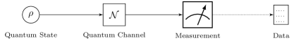
Figure 1: Schematic diagram of a quantum state $\rho$ passing through a quantum channel ${\mathcal{N}}$ prior to being measured.

Bayesian estimators for $\rho$ can be obtained by replacing $\Pr(\delta|\rho)$ with $\Pr(\delta|{\mathcal{N}}(\rho))$ in (6) and (8). The MAP estimate in (10) becomes

$$\hat{\rho}_{\text{MAP}}=\underset{\rho\in{\mathcal{S}}}{\text{argmax}}\;[\log p(\delta|{\mathcal{N}}(\rho))+\log p(\rho)],$$ (18)

In addition the MAP estimate of the state coming out of the channel can be shown to be,

$$\hat{\sigma}_{\text{MAP}}={\mathcal{N}}(\hat{\rho}_{\text{MAP}}).$$ (19)

The above construction is quite general. There is no restriction on ${\mathcal{N}}$, the form of $\Pr(\delta|\rho)$, $p(\rho)$, or the size of the quantum system $d$. Because ${\mathcal{N}}$ is a linear map, if $\log\Pr(\delta|\rho)$ is concave in $\rho$ so is $\log\Pr(\delta|{\mathcal{N}}(\rho))$. Thus when the tools of convex optimization allow an efficient calculation of the MAP estimate in (10) the same will be true of (18). Since the MLE, MLME, and the HMLE are special cases of MAP, they can likewise be adapted to the the noisy setting.

Note that the Gaussian noise models considered in [17, 18] are quite different: they are not based on a noisy channel, but instead on a special form of $\Pr(\delta|\rho)$.

4.1 Example

Let $\{\sigma_{s}\}_{s\in\{x,y,z\}}$ be the Pauli matrices. A qubit density operator can be expressed in the Bloch parametrization,

$$\rho(\textbf{r})=\frac{1}{2}(\mathbb{I}+\textbf{r}.\vec{\sigma}):=\frac{1}{2}(\mathbb{I}+r_{x}\sigma_{x}+r_{y}\sigma_{y}+r_{z}\sigma_{z}),$$ (20)

where the Bloch vector $\textbf{r}=(r_{x},r_{y},r_{z})$, with norm $|\textbf{r}|$, belongs to the set of real variables $R=\{\textbf{r}\;||\textbf{r}|\leq 1\}$ called the Bloch ball. For doing tomography suppose $3N$ measurements, $N$ each in the eigenbasis $\{|+\rangle_{s},|-\rangle_{s}\}$ of $\{\sigma_{s}\}_{s\in\{x,y,z\}}$, are performed on identically prepared quantum systems, each described by the density operator $\rho$. The probability of observing $|+\rangle_{s}$,

$$p_{s}={\rm Tr}(\rho[+]_{s})=(1+r_{s})/2,\quad s\in\{x,y,z\},$$ (21)

where $[+]_{s}$ denotes the projector on $|+\rangle_{s}$. The measurement data set $\delta=\{n_{s},N-n_{s}\}_{s\in\{x,y,z\}}$, where $n_{s}$ denotes the number of times $|+\rangle_{s}$ is observed, has a probability

$$\Pr(\delta|\rho)=C_{\delta}\underset{s\in\{x,y,z\}}{\prod}p_{s}^{n_{s}}(1-p_{s})^{N-n_{s}},$$ (22)

where $C_{\delta}=(3N)!/(\prod_{s}n_{s}!(N-n_{s})!)$. Using (11) and (20), a simple MLE estimate

$$\hat{\rho}_{\text{MLE}}=\underset{\textbf{r}\in R}{\text{argmax}}\;\log\Pr(\delta|\rho(\textbf{r}))$$ (23)

can be obtained. However most tomography setups have noise. For example, when discussing noise in a nuclear magnetic resonance (NMR) experiment [24, 25, 26] one may use the model described in Fig. 1, where the channel ${\mathcal{N}}$, acting over time $t$ represents the combined action of two channels, the generalized amplitude damping ($T_{1}$) channel,

$${\mathcal{A}}(\rho)=\sum_{i}A_{i}\rho A_{i}^{{\dagger}},$$ (24)

where,

$$A_{0}=\sqrt{p}\begin{pmatrix}1&0\\ 0&\sqrt{1-\gamma}\end{pmatrix},A_{1}=\sqrt{p}\begin{pmatrix}0&\sqrt{\gamma}\\ 0&0\end{pmatrix},A_{2}=\sqrt{1-p}\begin{pmatrix}\sqrt{1-\gamma}&0\\ 0&1\end{pmatrix},A_{3}=\sqrt{1-p}\begin{pmatrix}0&0\\ \sqrt{\gamma}&0\end{pmatrix},$$ (25)

$p\in[0,1]$, is the probability of finding the qubit in the $|0\rangle$ state as $t\mapsto\infty$, $\gamma=1-e^{-t/T_{1}}$, $T_{1}$ is a time constant, and the phase damping ($T_{2}$) channel,

$${\mathcal{B}}(\rho)=\sum_{j}B_{j}\rho B_{j}^{\dagger},$$ (26)

where,

$$B_{0}=\begin{pmatrix}1&0\\ 0&\sqrt{1-\lambda}\end{pmatrix},B_{1}=\begin{pmatrix}0&0\\ 0&\sqrt{\lambda}\end{pmatrix},$$ (27)

$\lambda=1-e^{-t/T_{2}}$, and $T_{2}$ is a time constant, and ${\mathcal{N}}={\mathcal{A}}\circ{\mathcal{B}}={\mathcal{B}}\circ{\mathcal{A}}$ .

A MAP estimate which accounts for the noise, assuming a prior probability density independent of r (under this probability density function, equal volumes of the Bloch ball have equal probability), can be obtained by using (18) and (20),

$$\hat{\rho}_{\text{MAP}}=\underset{\textbf{r}\in R}{\text{argmax}}\;\log\Pr(\delta|{\mathcal{N}}(\rho(\textbf{r}))).$$ (28)

We perform numerical simulations to test performance of MLE and MAP in (23) and (28) respectively. There is no unique metric to assess how close an estimate $\hat{\rho}$ is to the actual $\rho$. The fidelity ${\mathcal{F}}(\rho,\hat{\rho})\equiv{\rm Tr}(\sqrt{\sqrt{\rho}\hat{\rho}\sqrt{\rho}})$ and trace distance ${\mathcal{D}}(\rho,\hat{\rho})\equiv\frac{1}{2}||\rho-\hat{\rho}||_{1}$ are, however popular choices. Various parameter choices for ${\mathcal{A}}$ and ${\mathcal{B}}$ are used in the simulation by fixing $p=1/2$, $T_{1}/T_{2}=10$ [26], $t=kT_{2}$ and varying $k\in\{0.25,.5,.75,1.0,1.5,2.0,2.5\}$. For any fixed $k$, we choose $2.5\times 10^{3}$ qubit states uniformly in the Bloch ball. For each state we simulate the construction of the MLE and MAP estimates for various $N$ values. By averaging over all qubit states we arrive at the average log-infidelity ($\log_{10}[1-{\mathcal{F}}(\rho,\hat{\rho})]$) and log-trace distance ($\log_{10}[{\mathcal{D}}(\rho,\hat{\rho})]$) of the MAP and MLE estimators (see Appendix for numerical techniques). For a fixed $k$, under both log-infidelity and log-trace distance, the behaviour of MAP and MLE estimators with the number of measurements ($3N$) is shown in Fig. 2.

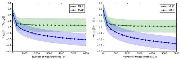
Figure 2: (Color online) Plot of the average log-infidelity and log-trace distance between the true and estimated state, against the number of measurements at $k=0.5$. The error bars represent one standard deviation. If the quantum channel ${\mathcal{N}}$ was perfect and the number of measurements was infinite, the log infidelity and log trace distance would be negative infinity for MAP and MLE. As the ordinate of the graph increases the performance of the estimator becomes worse.

Under both metrics, MAP and MLE show qualitatively different behaviour. As the number of measurements increases from a small value, for both metrics, the average MAP value decreases and the average MLE value decreases but settles to a fixed number. Thus, on average the MAP estimate always improves with the number of measurements while the MLE improves up to a point and then ceases to change. ${\mathcal{N}}$ becomes more noisy as $k$ increases and this causes both the MAP and MLE curves in each of the plots in Fig. 2 to shift upwards. The upward shift implies that for a fixed $N$ with increasing $k$, on average the MAP and MLE estimates become worse under both metrics. In the case of MAP this effect of increasing $k$ can be mitigated by increasing the number of measurements which on average improves the estimate, however this is not always possible for MLE whose average value, under both metrics becomes fixed beyond a certain number of measurements and this fixed value also increases with $k$. Under both metrics and for all $k$ values tested, when the number of measurements is modestly large (roughly greater than $300$ in our case), on average MAP outperforms MLE. As the number of measurements increases further the average MAP value becomes an order of magnitude better than average MLE value, and eventually the error bars (one standard deviation about the average value) on the MAP and MLE curves cease to overlap. Thus numerical evidence on qubits shows, that except when the number of measurements are low, on average there is an advantage of using a MAP estimator which accounts for noise over a standard MLE.

5 Conclusion

The maximum a posteriori probability (MAP) estimation framework for quantum state and process tomography introduced here combines a number of previous quantum state estimators, in particular the maximum likelihood, hedged maximum likelihood, and maximum likelihood-maximum entropy estimator, in a single framework using Bayesian methodology. In several cases of interest to quantum state tomography the MAP estimator becomes a convex optimization problem which should be numerically more tractable than the Bayes’ Mean Estimator. Using the Choi-Jamiołlkowski isomorphism, MAP estimation of quantum states can be extended to quantum channels, and the extension is expected to have similar advantages as the MAP estimate for quantum states. When the experimental noise can be represented by a known noisy channel preceding the measurement, the MAP estimator can be modified to take it into account and can be computed efficiently as long as the posterior probability density is log concave. Numerical results on qubits indicate that on average, such modifications can vastly improve estimates. Having a measure of reliability for any estimate is of significant value, and it would be interesting to construct such measures for the MAP estimate.

Appendix A Appendix. Convex Optimization over qubit density operators

Projected gradient descent is a very general iterative algorithm, used extensively for minimizing functions defined over convex sets. When the function is convex, successive function values obtained during the algorithm approach the global minimum. For some special convex sets, tools from convex analysis can be used to compute a bound on how close a given function value is to the global minimum. We provide an exposition of the projected gradient descent algorithm for minimizing any differentiable convex function over the set of qubit density operators, and illustrate a technique for checking how far a given function value is from the global minimum. Let $f:R\mapsto\mathbb{R}$ be a differentiable convex function, then

$$f(\textbf{x}^{*})=f^{*}=\underset{\textbf{x}\in R}{\min}\;f(\textbf{x}),$$ (29)

is called the optimization problem, with objective function $f$, optimal $\textbf{x}^{*}$ and optimum value $f^{*}$. Projected gradient descent begins with some point inside $R$, then iteratively takes steps to move to a new point with a lower function value. The algorithm halts when some stopping criterion is met. New points are chosen by moving along the negative gradient direction by an amount called the step size, such movements may take one outside the set $R$, in which case we project onto the boundary of the set. If x is a vector in $\mathbb{R}^{3}$ then its projection onto $R$,

$$P_{R}(\textbf{x})=\begin{cases}\textbf{x}/|\textbf{x}|\quad\text{if}\quad|\textbf{x}|>1\\ \textbf{x}\quad\text{otherwise}\end{cases}.$$ (30)

A pseudo code for projected gradient descent is given in algorithm 1.

Input : $\textbf{x}\in R$

Output : $\tilde{\textbf{x}}$ and $\tilde{f}$

1 while not stopping criterion do

2       $\textbf{d}=\nabla f(\textbf{x})$

3       $\textbf{y}_{t}=\textbf{x}-t\textbf{d}$

4       $\textbf{x}^{+}(t)=P_{R}(\textbf{y}(t))$

5       Choose step size $t^{*}$

6       $\textbf{x}=\textbf{x}^{+}(t^{*})$

7 end while

8return $\textbf{x},f(\textbf{x})$

Algorithm 1 Projected gradient descent

There are several different ways of choosing a step size and a stopping criterion. We select the step size by using a method called backtracking line search. Let

$$G_{t}(\textbf{x})\equiv(\textbf{x}-\textbf{x}^{+}(t))/t$$ (31)

be the generalized gradient at x for step size $t$. A pseudo code for backtracking, to be used as a subroutine in algorithm 1 is provided in algorithm 2.

Input : $\beta\in(0,1)$

Output : $t^{*}$

1 Let $t=1$

2 while $f(\textbf{x}^{+}(t))>f(\textbf{x})-t\langle\textbf{d},G_{t}(\textbf{x})\rangle+\frac{t}{2}|G_{t}(\textbf{x})|^{2}$ do

3       $t=\beta t$

4      

5 end while

6return $t$

Algorithm 2 Backtracking line search

Backtracking line search ensures that the function decreases by at least $t^{*}|G_{t^{*}}(\textbf{x})|^{2}/2$ in each iteration [29]. One possible stopping criterion is to check whether the function hasn’t decreased appreciably over the past few iterations or $|G_{t^{*}}(\textbf{x})|$ is greater than a small constant. At any point $\textbf{x}\in R$, the surrogate duality gap [30]

$$g(\textbf{x})=\underset{\textbf{r}\in R}{\max}\;\langle\nabla f(\textbf{x}),\textbf{x}-\textbf{r}\rangle$$ (32)

upper bounds $|f(\textbf{x})-f^{*}|$ and provides a measure of how close a function value at x is to the global minimum value. Due to the simple structure of the set of qubit density operators, the surrogate duality gap can be easily computed. Let $\nabla F(\textbf{x})=\nabla f(\textbf{x}).\vec{\sigma}$ be a matrix, $\lambda_{\min}(\nabla F(\textbf{x}))$ be its smallest eigenvalue, then

$$g(\textbf{x})=\langle\nabla f(\textbf{x}),\textbf{x}\rangle-\lambda_{\min}(\nabla F(\textbf{x})).$$ (33)

Given the ease of computing $g(\textbf{x})$, checking whether its value is greater that a small constant also serves as a good stopping criterion. Once algorithm 1 converges and returns some $(\tilde{\textbf{x}},f(\tilde{\textbf{x}}))$, computing $g(\tilde{\textbf{x}})$ gives an estimate of how far $f(\tilde{\textbf{x}})$ is from $f^{*}$.

The projected gradient algorithm discussed above can be used to solve optimization problems in Eq. (23) and (28) to obtain $\hat{\rho}_{\text{MLE}}$ and $\hat{\rho}_{\text{MAP}}$ respectively. The gradient of the objective function in these optimization problems can be computed analytically. Let $\textbf{r}=(r_{x},r_{y},r_{z})$ be a Bloch vector for a qubit density operator $\rho$, then upto local unitaries at the input and output of a qubit channel ${\mathcal{N}}$, the Bloch vector $\textbf{r}^{\prime}$ for ${\mathcal{N}}(\rho)$ can always be written as $\textbf{r}^{\prime}=(l_{x}r_{x}+t_{x},l_{y}r_{y}+t_{y},l_{z}r_{z}+t_{z})$ [31]. When ${\mathcal{N}}={\mathcal{I}}$

$$l_{s}=1,t_{s}=0,\;s\in\{x,y,z\},$$ (34)

when ${\mathcal{N}}={\mathcal{A}}\circ{\mathcal{B}}$ (see Eq. (24) and (26))

$$l_{x}=l_{y}=\sqrt{(1-\lambda)(1-\gamma)},\;l_{z}=1-\gamma,t_{x}=t_{y}=0,\;\text{and}\;t_{z}=\gamma(2p-1).$$ (35)

The gradient of the function on the right hand side in Eq. (28) can be obtained using

$$\frac{\partial}{\partial r_{s}}\log\Pr(\delta|{\mathcal{N}}(\rho(\textbf{r})))=\frac{l_{s}}{2}\big{(}\frac{n_{s}}{p_{s}}-\frac{N-n_{s}}{1-p_{s}}\big{)},\quad s\in\{x,y,z\}.$$ (36)

Choosing ${\mathcal{N}}={\mathcal{I}}$ gives the gradient of the function in the right side of Eq. (23). A python implementation of projected gradient descent and surrogate duality gap computation over qubits, including a code that simulates the tomography reconstruction and generates plots for Fig. 2 is publicly available [32].

References

- [1] Z. Hradil. Quantum-state estimation. Phys. Rev. A, 55:R1561–R1564, Mar 1997.
- [2] Robin Blume-Kohout. Hedged maximum likelihood quantum state estimation. Phys. Rev. Lett., 105:200504, Nov 2010.
- [3] Yong Siah Teo, Huangjun Zhu, Berthold-Georg Englert, Jaroslav Řeháček, and Zden ěk Hradil. Quantum-state reconstruction by maximizing likelihood and entropy. Phys. Rev. Lett., 107:020404, Jul 2011.
- [4] David Gross, Yi-Kai Liu, Steven T. Flammia, Stephen Becker, and Jens Eisert. Quantum state tomography via compressed sensing. Phys. Rev. Lett., 105:150401, Oct 2010.
- [5] Yong Siah Teo. Introduction to Quantum-State Estimation. World Scientific, 2015.
- [6] Robin Blume-Kohout. Robust error bars for quantum tomography. arXiv:1202.5270, 2012
- [7] Christopher Ferrie and Robin Blume-Kohout. Minimax Quantum Tomography: Estimators and Relative Entropy Bounds. Physical Review Letters, 116(9):090407, mar 2016.
- [8] Matthias Christandl and Renato Renner. Reliable quantum state tomography. Physical Review Letters, 109(12), 2012.
- [9] Philippe Faist and Renato Renner. Practical and reliable error bars in quantum tomography. Phys. Rev. Lett., 117:010404, Jul 2016.
- [10] Aaron C. Chan, Kazuhiro Kurokawa, Shuichi Makita, Young-Joo Hong, Arata Miyazawa, Masahiro Miura, and Yoshiaki Yasuno, Quantitative optical coherence tomography by maximum a-posteriori estimation of signal intensity Proc. SPIE 9697, Optical Coherence Tomography and Coherence Domain Optical Methods in Biomedicine XX, 96971W (8 March 2016)
- [11] Doga Gürsoy, Tekin Biçer, Jonathan D. Almer, Raj Kettimuthu, Stuart R. Stock, and Francesco De Carlo. Maximum a posteriori estimation of crystallographic phases in x-ray diffraction tomography. Philosophical transactions. Series A, 373(2043):20140392, Jun 2015.
- [12] Robin Blume-Kohout. Optimal, reliable estimation of quantum states. New Journal of Physics, 12(4):043034, Apr 2010.
- [13] Stephen Boyd and Lieven Vandenberghe. Convex Optimization. Cambridge University Press, 2004.
- [14] Jiangwei Shang, Zhengyun Zhang, and Hui Khoon Ng. Superfast maximum-likelihood reconstruction for quantum tomography. Phys. Rev. A, 95:062336, Jun 2017.
- [15] Eliot Bolduc, George C. Knee, Erik M. Gauger, and Jonathan Leach. Projected gradient descent algorithms for quantum state tomography. npj Quantum Information, 3(1):44, 2017.
- [16] George C. Knee, Eliot Bolduc, Jonathan Leach, and Erik M. Gauger. Quantum process tomography via completely positive and trace-preserving projection. Phys. Rev. A, 98:062336, Dec 2018.
- [17] John A. Smolin, Jay M. Gambetta, and Graeme Smith. Efficient Method for Computing the Maximum-Likelihood Quantum State from Measurements with Additive Gaussian Noise. Physical Review Letters, 108(7):070502, Feb 2012.
- [18] Harpreet Singh, Arvind, and Kavita Dorai. Constructing valid density matrices on an NMR quantum information processor via maximum likelihood estimation. Physics Letters A, 380(38):3051–3056, Sep 2016.
- [19] Karol Zyczkowski and Hans-Jürgen Sommers. Induced measures in the space of mixed quantum states. Journal of Physics A: Mathematical and General, 34(35):7111, 2001.
- [20] Man-Duen Choi. Completely positive linear maps on complex matrices. Linear Algebra and its Applications, 10(3):285 – 290, 1975.
- [21] Patrick J. Coles, Li Yu, Vlad Gheorghiu, and Robert B. Griffiths. Information-theoretic treatment of tripartite systems and quantum channels. Phys. Rev. A, 83:062338, Jun 2011.
- [22] Debbie W. Leung. Choi’s proof as a recipe for quantum process tomography. Journal of Mathematical Physics, 44(2):528–533, 2003.
- [23] Isaac L.Chuang and M. A. Nielsen. Prescription for experimental determination of the dynamics of a quantum black box. Journal of Modern Optics, 44(11-12):2455–2467, 1997.
- [24] Lieven M. K. Vandersypen, Matthias Steffen, Gregory Breyta, Costantino S. Yannoni, Mark H. Sherwood, and Isaac L. Chuang. Experimental realization of shor’s quantum factoring algorithm using nuclear magnetic resonance. Nature, 414:883, Dec 2001.
- [25] M. S. Anwar, J. A. Jones, D. Blazina, S. B. Duckett, and H. A. Carteret. Implementation of nmr quantum computation with parahydrogen-derived high-purity quantum states. Phys. Rev. A, 70:032324, Sep 2004.
- [26] Harpreet Singh, Arvind, and Kavita Dorai. Evolution of tripartite entangled states in a decohering environment and their experimental protection using dynamical decoupling. Phys. Rev. A, 97:022302, Feb 2018.
- [27] J. Towns, T. Cockerill, M. Dahan, I. Foster, K. Gaither, A. Grimshaw, V. Hazlewood, S. Lathrop, D. Lifka, G. D. Peterson, R. Roskies, J. R. Scott, and N. Wilkins-Diehr. Xsede: Accelerating scientific discovery. Computing in Science & Engineering, 16(5):62–74, Sept.-Oct. 2014.
- [28] Nicholas A. Nystrom, Michael J. Levine, Ralph Z. Roskies, and J. Ray Scott. Bridges: A uniquely flexible hpc resource for new communities and data analytics. In Proceedings of the 2015 XSEDE Conference: Scientific Advancements Enabled by Enhanced Cyberinfrastructure, XSEDE ’15, pages 30:1–30:8, New York, NY, USA, 2015. ACM.
- [29] Larry Armijo. Minimization of functions having lipschitz continuous first partial derivatives. Pacific J. Math., 16(1):1–3, 1966.
- [30] Martin Jaggi. Revisiting frank-wolfe: Projection-free sparse convex optimization. In Sanjoy Dasgupta and David McAllester, editors, Proceedings of the 30th International Conference on Machine Learning, volume 28 of Proceedings of Machine Learning Research, pages 427–435, Atlanta, Georgia, USA, 17–19 Jun 2013. PMLR.
- [31] Robert B. Griffiths. Quantum computation and quantum information theory course notes: Quantum channels, kraus operators, povms. http://quantum.phys.cmu.edu/QCQI/index.html, Oct 2013.
- [32] Vikesh Siddhu. Python implementation of map estimation over qubits density operators. https://github.com/vsiddhu/MAPqubit.git, January 2018.