A General Convergence Result for
Mirror Descent with Armijo Line Search

Abstract

Existing convergence guarantees for the mirror descent algorithm require the objective function to have a bounded gradient or be smooth relative to a Legendre function. The bounded gradient and relative smoothness conditions, however, may not hold in important applications, such as quantum state tomography and portfolio selection. In this paper, we propose a local version of the relative smoothness condition as a generalization of its existing global version, and prove that under this local relative smoothness condition, the mirror descent algorithm with Armijo line search always converges. Numerical results showed that, therefore, the mirror descent algorithm with Armijo line search was the fastest guaranteed-to-converge algorithm for quantum state tomography, empirically on real data-sets.

1 Introduction

Consider a constrained convex optimization problem:

$$f^{\star}=\min_{x}\set{f(x)}{x\in\mathcal{X}},$$ (P)

where $f$ is a convex differentiable function, and $\mathcal{X}$ is a convex closed set in $\mathbb{R}^{d}$. We assume that $f^{\star}>-\infty$.

The mirror descent algorithm is standard for solving such a constrained convex optimization problem [6, 32]. Given an initial iterate $x_{0}\in\mathcal{X}$, the mirror descent algorithm iterates as

$$x_{k+1}=\operatorname*{\arg\min}_{x}\Set{\braket{\nabla f(x_{k}),x-x_{k}}+\alpha_{k}D_{h}(x,x_{k})}{x\in\mathcal{X}}\,,\quad\forall k\in\mathbb{N}\,,$$ (1)

for some convex differentiable function $h$ and a properly chosen sequence of step sizes $\set{\alpha_{k}}$, where $D_{h}$ denotes the Bregman divergence induced by $h$:

$$D_{h}(z_{2},z_{1}):=h(z_{2})-\left[h(z_{1})+\braket{\nabla h(z_{1}),z_{2}-z_{2}}\right],\quad\forall(z_{2},z_{2})\in\operatorname{\mathrm{dom}}h\times\operatorname{\mathrm{dom}}\nabla h\,.$$

With a proper choice of the funciton $h$, the mirror descent algorithm can have an almost dimension-independent convergence rate guarantee, or lower per-iteration computational complexity. A famous example is the exponentiated gradient method, which enjoys both benefits [25, 26]. The exponentiated gradient method corresponds to the mirror descent algorithm with $h$ being the negative Shannon entropy.

Convergence of the mirror descent algorithm has been established under the following two conditions on the objective function.

1. Bounded gradient: There exists some $L>0$, such that

   $$\|\nabla f(x)\|\leq L,\quad\forall x\in\mathcal{X},$$

   for some norm $\|\cdot\|$ [6, 32]

2. Relative smoothness: There exist some $L>0$ and a convex differentiable function $h$, such that

   $$f(y)\leq f(x)+\braket{\nabla f(x),y-x}+LD_{h}(y,x),\quad\forall x,y\in\mathcal{X},$$

   where $D_{h}$ denotes the Bregman divergence induced by $h$ [2, 3, 31].

These conditions may not hold, or introduce undesirable computational burdens for some applications. Quantum state tomography is one such instance.

Example 1

Quantum state tomography (QST) is the task of estimating the state of qubits (quantum bits) given measurement outcomes [36]; this task is essential to calibrating quantum computation devices. Numerically, it corresponds to minimizing the function

$$f_{\text{QST}}(x):=-\sum_{i=1}^{n}\log\operatorname{\mathrm{Tr}}(M_{i}x),$$

for given positive semi-definite matrices $M_{i}$, on the set of quantum density matrices

$$\mathcal{D}:=\Set{x\in\mathbb{C}^{d\times d}}{x\geq 0,\operatorname{\mathrm{Tr}}(x)=1}.$$ (2)

The dimension $d$ equals $2^{q}$, where $q$ is the number of qubits (quantum bits). _□

Notice that the diagonal of a density matrix in $\mathbb{R}^{d\times d}$ must belong to the probability simplex in $\mathbb{R}^{d}$; therefore, a density matrix can be viewed as a matrix analogue of a probability distribution. Regarding this observation, it is natural to consider the matrix version of the exponentiated gradient method, for which the Shannon entropy is replaced by its matrix analogue called the von Neumann entropy [11, 40]. Unfortunately, the following is easily checked.

Proposition 1

The gradient of the function $f_{\text{QST}}$ is not bounded. The function $f_{\text{QST}}$ is not smooth relative to the von Neumann entropy. _□

A proof is given in Section A.

Another popular choice of the function $h$ is Burg’s entropy. The resulting mirror descent algorithm iterates as

$$x_{k+1}=\left(x_{k}^{-1}+\alpha_{k}\nabla f(x_{k})\right)^{-1}\,,\quad\forall k\in\mathbb{N}\,,$$

where $\alpha_{k}$ is chosen such that $\operatorname{\mathrm{Tr}}(x_{k+1})=1$ [28]. The numerical search for $\alpha_{k}$ yields high per-iteration computational complexity of the mirror descent algorithm.

We note that in terms of the objective functions and constraint sets, positron emission tomography, optimal portfolio selection, and non-negative linear inverse problems are essentially vector analogues of QST [12, 14, 41]. The same issues we have discussed above remain in these applications, though the computational burden due to the Burg entropy may be relatively minor in these vector analogues.

To address “non-standard” applications like QST, we relax the condition on the objective function. Specifically, we propose a novel localized version of the relative smoothness condition. The local relative smoothness condition does not involve any parameter, in comparison to the bounded gradient and (global) relative smoothness conditions. Therefore, we do not seek for a closed-form expression for the step sizes; instead, we consider selecting the step sizes adaptively by Armijo line search.

1.1 Related work

The mirror descent algorithm was introduced in [32]. The formulation (1) was proposed in [6], which is equivalent to the original one under standard assumptions. The interior gradient method studied in [2] is also of the form (1); the difference lies in the technical conditions. Standard convergence analyses of the mirror descent, as discussed above, assume either bounded gradient or relative smoothness [2, 3, 6, 31, 32]. The exponentiated gradient method was proposed in [26]; it is also known as the entropic mirror descent [6].

For quantum state tomography, there are few guaranteed-to-converge optimization algorithms. The $R\rho R$ algorithm was proposed as an analogue of the expectation maximization (EM) algorithm [23], but does not always converge [42]. The diluted $R\rho R$ algorithm is a variant of the $R\rho R$ algorithm; it guarantees convergence by exact line search [42]. The Frank-Wolfe algorithm converges with a step size selection rule slightly different from the standard one [35]. The SCOPT algorithm proposed in [39], a proximal gradient method for composite self-concordant minimization, also converges, as the logarithmic function is a standard instance of a self-concordant function. The numerical results in Section 6, unfortunately, showed that the convergence speeds of the diluted $R\rho R$, Frank-Wolfe, and SCOPT algorithms are not satisfactory on real data-sets.

For the vector analogues of QST mentioned above, the standard approach is the EM algorithm [14, 18, 41]. The algorithm is also known as the Richardson-Lucy (RL) algorithm in astronomy and microscopy (see, e.g., [7]). The numerical results in Section 6 showed that the EM algorithm is slow on real data-sets for portfolio selection. There are faster accelerated versions of the EM algorithm based on line search, but they lack convergence guarantees [7]. Guranteed-to-converge variable metric methods with line search were proposed in [9, 10], but they involve an infinite number of parameters to be properly tuned.

Armijo line search was proposed in [1], for minimizing functions with Lipschitz gradients. The formulation of Armijo line search studied in this paper is the generalized version proposed in [8].

1.2 Contributions

We propose a novel local relative smoothness condition, and show that the condition is satisfied by a large class of objective functions. The main result is Theorem 1, which establishes convergence of the mirror descent algorithm with Armijo line search under the local relative smoothness condition. Numerical results showed that, because of Theorem 1, the exponentiated gradient method with Armijo line search was the fastest guaranteed-to-converge algorithm for QST, empirically on real data-sets. To the best of our knowledge, even for globally relatively smooth objective functions, convergence of mirror descent with Armijo line search has not been proven; Theorem 1 provides the first convergence guarantee for this setup.

2 Mirror Descent with Armijo Line Search

Let $h$ be a convex differentiable function strictly convex on $\mathcal{X}$. The corresponding Bregman divergence is given by

$$D_{h}(z_{2},z_{1}):=h(z_{2})-\left[h(z_{1})+\braket{\nabla h(z_{1}),z_{2}-z_{2}}\right],\quad\forall(z_{2},z_{2})\in\operatorname{\mathrm{dom}}h\times\operatorname{\mathrm{dom}}\nabla h.$$

Because of the strict convexity of $h$, it holds that $D_{h}(z_{2},z_{1})\geq 0$, and $D_{h}(z_{2},z_{1})=0$ if and only if $z_{2}=z_{1}$.

Define $\tilde{\mathcal{X}}:=\mathcal{X}\cap\operatorname{\mathrm{dom}}\nabla f\cap\operatorname{\mathrm{dom}}\nabla h$. The corresponding mirror descent algorithm starts with some $x_{0}\in\tilde{\mathcal{X}}$, and iterates as

$$x_{k}=x_{k-1}(\alpha_{k}):=\operatorname*{\arg\min}_{x}\Set{\alpha_{k}\braket{\nabla f(x_{k-1}),x-x_{k-1}}+D_{h}(x,x_{k-1})}{x\in\mathcal{X}},\quad\forall k\in\mathbb{N},$$

where $\alpha_{k}$ denotes the step size. To ensure that the mirror descent algorithm is well-defined, we will assume the following throughout this paper.

Assumption 1

For every $x\in\tilde{\mathcal{X}}$ and $\alpha\geq 0$, $x(\alpha)$ is uniquely defined and lies in $\tilde{\mathcal{X}}$.

There are several sufficient conditions that guarantee Assumption 1, but in practice, it is typically easier to directly check Assumption 1. The interested reader is referred to, e.g., [3, 4] for the details.

Algorithm 1 Mirror Descent with Armijo Line Search

1:$\bar{\alpha}>0$, $r\in(0,1)$, $\tau\in(0,1)$, $x_{0}\in\mathcal{X}_{h}$

2:for $k=1,2,\ldots$ do

3:     $\alpha_{k}\leftarrow\bar{\alpha}$

4:     while $\tau\Braket{\nabla f(x_{k-1}),x_{k-1}(\alpha_{k})-x_{k-1}}+f(x_{k-1})<f(x_{k-1}(\alpha_{k}))$ do

5:         $\alpha_{k}\leftarrow r\alpha_{k}$

6:     end while

7:     $x_{k}\leftarrow x_{k-1}(\alpha_{k})$

8:end for

We consider choosing the step sizes by the Armijo rule. Let $\bar{\alpha}>0$ and $r,\tau\in(0,1)$. The Armijo rule outputs $\alpha_{k}=r^{j}\bar{\alpha}$ for every $k$, where $j$ is the least non-negative integer such that

$$f(x_{k-1}(r^{j}\bar{\alpha}))\leq f(x_{k-1})+\tau\braket{\nabla f(x_{k-1}),x_{k-1}(r^{j}\bar{\alpha})-x_{k-1}}.$$

The Armijo rule can be easily implemented by a while-loop, as shown in Algorithm 1.

3 Local Relative Smoothness

In this section, we introduce the local relative smoothness condition, and provide a detailed discussion. In particular, we provide some practical approaches to checking the local relative smoothness condition, alone with concrete examples illustrating when the practical approaches can and cannot be applied.

Roughly speaking, the local relative smoothness condition asks that for every point, there exists a neighborhood on which $f$ is relatively smooth.

Definition 1

We say that $f$ is locally smooth relative to $h$ on $\mathcal{X}$, if for every $x\in\mathcal{X}\cap\operatorname{\mathrm{dom}}f$, there exist some $L_{x}>0$ and $\varepsilon_{x}>0$, such that

$$f(z_{2})\leq f(z_{1})+\braket{\nabla f(z_{1}),z_{2}-z_{1}}+L_{x}D_{h}(z_{2},z_{1}),\quad\forall z_{1},z_{2}\in\mathcal{B}_{\varepsilon_{x}}(x)\cap\tilde{\mathcal{X}},$$ (3)

where $\mathcal{B}_{\varepsilon_{x}}(x)$ denotes the ball centered at $x$ of radius $\varepsilon_{x}$ with respect to a norm. _□

If we set $h:x\mapsto(1/2)\|x\|_{2}^{2}$, then (3) becomes

$$f(z_{2})\leq f(z_{1})+\braket{\nabla f(z_{1}),z_{2}-z_{1}}+\frac{L_{x}}{2}\|z_{2}-z_{1}\|_{2}^{2},\quad\forall z_{1},z_{2}\in\mathcal{B}_{\varepsilon_{x}}(x)\cap\tilde{\mathcal{X}},$$

This is indeed the the locally Lipschitz gradient condition in literature.

Lemma 1

The following two statements are equivalent.

1. The function $f$ is locally smooth relative to $h:x\mapsto(1/2)\|x\|_{2}^{2}$ on $\mathcal{X}$.

2. Its gradient $\nabla f$ is locally Lipschitz on $\operatorname{\mathrm{int}}\tilde{\mathcal{X}}$; that is, for every $x\in\mathcal{X}\cap\operatorname{\mathrm{dom}}f$, there exists some $L_{x}>0$ and $\varepsilon_{x}>0$, such that

   $$\|\nabla f(z_{2})-\nabla f(z_{1})\|_{2}\leq L_{x}\|z_{2}-z_{1}\|_{2},\quad\forall z_{1},z_{2}\in\mathcal{B}_{\varepsilon_{x}}(x)\cap\tilde{\mathcal{X}}.$$

_□

The proof of Lemma 1 is standard; we give it in Appendix B.

It is already known that the local Lipschitz gradient condition lies strictly between the following two conditions.

1. The function $f$ is differentiable.

2. The gradient of $f$ is (globally) Lipschitz.

See [22, 24] for the details.

The following result provides a practical approach to checking the local Lipschitz gradient condition.

Proposition 2

Suppose that $\operatorname{\mathrm{dom}}f\cap\mathcal{X}$ is relatively open in $\mathcal{X}$, and $f$ is twice continuously differentiable on $\operatorname{\mathrm{dom}}f\cap\mathcal{X}$. Then $f$ is locally smooth relative to $h(\cdot):=(1/2)\|\cdot\|_{2}^{2}$ on $\mathcal{X}$. _□

Proof

Recall the definition of relative openness: For every $x$ in $\operatorname{\mathrm{dom}}f\cap\mathcal{X}$, there exists some $\varepsilon_{x}$ such that $\mathcal{B}_{\varepsilon_{x}}(x)\cap\mathcal{X}\subseteq\operatorname{\mathrm{dom}}f\cap\mathcal{X}$. Notice that the largest eigenvalue of $\nabla^{2}f$ is a continuous function on $\mathcal{B}_{\varepsilon_{x}}(x)\cap\mathcal{X}$; by the extreme value theorem, there exists some $L_{x}$ such that $\nabla^{2}f(z)\leq L_{x}I$ for every $z\in\mathcal{B}_{\varepsilon_{x}}(x)\cap\mathcal{X}$. For every $z_{1},z_{2}\in\mathcal{B}_{\varepsilon_{x}}\cap\tilde{\mathcal{X}}$, we use Taylor’s formula with the integral remainder and write

$$f(z_{2}) =f(z_{1})+\braket{\nabla f(z_{1}),z_{2}-z_{1}}+\int_{0}^{1}\int_{0}^{t}\braket{\nabla^{2}f(z_{1}+\tau(z_{2}-z_{1}))(z_{2}-z_{1}),z_{2}-z_{1}}\,\mathrm{d}\tau\,\mathrm{d}t$$

$$\leq f(z_{1})+\braket{\nabla f(z_{1}),z_{2}-z_{1}}+\int_{0}^{1}\int_{0}^{t}L_{x}\|z_{2}-z_{1}\|_{2}^{2}\,\mathrm{d}\tau\,\mathrm{d}t$$

$$=f(z_{1})+\braket{\nabla f(z_{1}),z_{2}-z_{1}}+\frac{L_{x}}{2}\|z_{2}-z_{1}\|_{2}^{2},$$

which proves the proposition. _■

Corollary 1

If $f$ is twice continuously differentiable on $\mathcal{X}$, then it is locally smooth relative to $h(\cdot):=(1/2)\|\cdot\|_{2}^{2}$ on $\mathcal{X}$. _□

Indeed, under the setting of Corollary 1, the function $f$ has a bounded Hessian by the extreme value theorem, and hence is smooth relative to $h(\cdot):=(1/2)\|\cdot\|_{2}^{2}$, i.e., the function satisfies the standard smoothness assumption in literature [33]; then most existing convergence results for first-order optimization algorithms apply. To derive an upper bound of the Lipschitz parameter, however, may be non-trivial. Moreover, there are cases where Corollary 1 does not apply, while Proposition 2 is applicable. Below is an example.

Example 2

Set $f(x):=-\log(x_{1})-\log(x_{2})$ for every $x:=(x_{1},x_{2})\in\mathbb{R}^{2}$. Set $\mathcal{X}$ to be the positive orthant. Then $f$ is not twice continuously differentiable on $\mathcal{X}$; for example, $\nabla^{2}f(1,0)$ does not exist. However, Proposition 2 is applicable—$\operatorname{\mathrm{dom}}f\cap\mathcal{X}$ is relatively open in $\mathcal{X}$ as $\operatorname{\mathrm{dom}}f$ is open, and it is easily checked that $f$ is twice continuously differentiable on $\operatorname{\mathrm{dom}}f\cap\mathcal{X}$. _□

Note that the local Lipschitz gradient condition is not always applicable.

Example 3

Set $f(x):=x_{1}\log(x_{1})+x_{2}\log(x_{2})$ for every $x:=(x_{1},x_{2})\in\mathbb{R}^{2}$, where we adopt the convention that $0\log 0:=0$. Set $\mathcal{X}$ to be the probability simplex in $\mathbb{R}^{2}$. Then $f$ is not locally smooth relative to $h(\cdot):=(1/2)\|\cdot\|_{2}^{2}$. For example, the point $x=(0,1)$ lies in $\operatorname{\mathrm{dom}}f\cap\mathcal{X}$, while $\nabla f$ is unbounded around $(0,1)$. However, it is obvious that $f$ is locally smooth relative to the negative Shannon entropy—indeed, $f$ itself is the negative Shannon entropy function. _□

A standard setting for the mirror descent algorithm requires the following [2, 6, 25].

Assumption 2

The function $h$ is strongly convex with respect to a norm $\|\cdot\|$ on $\mathcal{X}$; that is, there exists some $\mu>0$, such that

$$D_{h}(z_{2},z_{1})\geq\frac{\mu}{2}\|z_{2}-z_{1}\|^{2},\quad\forall(z_{2},z_{1})\in(\operatorname{\mathrm{dom}}h\cap\mathcal{X})\times(\operatorname{\mathrm{dom}}\nabla h\cap\mathcal{X}).$$

If $f$ is locally smooth relative to $h(x):=(1/2)\|x\|_{2}^{2}$, it is also locally smooth relative to any function $\tilde{h}$ strongly convex on $\mathcal{X}$ with respect to a norm $\|\cdot\|$—if for some $L>0$ and $z_{1},z_{2}\in\operatorname{\mathrm{dom}}\nabla\tilde{h}\times\operatorname{\mathrm{dom}}\tilde{h}$, it holds that

$$f(z_{2})\leq f(z_{1})+\braket{\nabla f(z_{1}),z_{2}-z_{1}}+\frac{L}{2}\|z_{2}-z_{1}\|_{2}^{2},$$

then we have

$$f(z_{2})\leq f(z_{1})+\braket{\nabla f(z_{1}),z_{2}-z_{1}}+\frac{CL}{\mu}D_{\tilde{h}}(z_{2},z_{1}),$$

for some $C>0$ such that $\|\cdot\|_{2}\leq C\|\cdot\|$, which exists because all norms on a finite-dimensional space are equivalent. Therefore, with Assumption 2, it suffices to check for local smoothness relative to $h(x):=(1/2)\|x\|_{2}^{2}$.

Example 4

Suppose that the constraint set $\mathcal{X}$ is the probability simplex. By Pinsker’s inequality, the negative Shannon entropy is strongly convex on $\mathcal{X}$ with respect to the $\ell_{1}$-norm [17]. By the discussion above and Corollary 1, any convex objective function that is twice continuously differentiable on $\mathcal{X}$ is locally smooth relative to the negative Shannon entropy. _□

It is possible that Assumption 2 does not hold, while we have local relative smoothness.

Example 5

Consider the function $f$ as defined in Example 2. Set $h:=f$, the Burg entropy. Then obviously, $f$ is smooth—and hence locally smooth—relative to $h$. However, if we set $\mathcal{X}$ to be the positive orthant, $h$ is not strongly convex on $\mathcal{X}$. _□

4 Main Result

The main result of this paper, the following theorem, says that the mirror descent algorithm with Armijo line search is well-defined, and guaranteed to converge, given assumptions discussed above.

Theorem 1

Suppose that Assumption 1 holds. Suppose that $\operatorname{\mathrm{dom}}f\cap\mathcal{X}\subseteq\operatorname{\mathrm{dom}}h\cap\mathcal{X}$, and $f$ is locally smooth relative to $h$. Then the following hold.

1. The Armijo line search procedure terminates in finite steps.

2. The sequence $\set{f(x_{k})}$ is non-increasing.

3. The sequence $\set{f(x_{k})}$ converges to $f^{\star}$, if $\set{x_{k}}$ is bounded.

_□

Boundedness of the sequence $\set{x_{k}}$ holds, for example, when the constraint set $\mathcal{X}$ or level set $\set{x\in\mathcal{X}}{f(x)\leq f(x_{0})}$ is bounded. A sufficient condition for the latter case is coercivity—a function is called coercive, if for every sequence $\set{x_{k}}$ such that $\|x_{k}\|\to+\infty$, we have $f(x_{k})\to+\infty$ (see, e.g., [5]).

5 Proof of Theorem 1

The proof of Theorem 1 stems from standard arguments (see, e.g., [2]), showing that the mirror descent algorithm converges, as long as the step sizes $\alpha_{k}$ are bounded away from zero. However, without any global parameter of the objective function, we are not able to provide an explicit lower bound for all step sizes as in [2]. We solve this difficulty by proving the existence of a strictly positive lower bound, for all but a finite number of the step sizes.

The following result shows that for every $x\in\tilde{\mathcal{X}}$, $x(\alpha)$ can be arbitrarily close to $x$ by setting $\alpha$ very small. This result is so fundamental in our analysis that we will use it without explicitly mentioning it.

Lemma 2

The function $x(\alpha)$ is continuous in $\alpha$ for every $x\in\tilde{\mathcal{X}}$. _□

Proof

Apply Theorem 7.41 in [38]. _■

For ease of presentation, we put the proofs of some technical lemmas in Section C.

5.1 Proof of Statement 1

Statement 1 follows from the following lemma.

Lemma 3

For every $x\in\tilde{\mathcal{X}}$, there exists some $\alpha_{x}>0$, such that

$$f(x(\alpha))\leq f(x)+\tau\braket{\nabla f(x),x(\alpha)-x},\quad\forall\alpha\in(0,\alpha_{x}].$$ (4)

_□

Proof

We write (4) equivalently as

$$f(x(\alpha))-\left[f(x)+\braket{\nabla f(x),x(\alpha)-x}\right]\leq-(1-\tau)\braket{\nabla f(x),x(\alpha)-x},\quad\forall\alpha\in(0,\alpha_{x}].$$

By the local relative smoothness condition, it suffices to check

$$L_{x}D_{h}(x(\alpha),x)\leq-(1-\tau)\braket{\nabla f(x),x(\alpha)-x},\quad\forall\alpha\in(0,\alpha_{x}].$$

By Lemma 7, it suffices to check

$$\alpha L_{x}D_{h}(x(\alpha),x)\leq(1-\tau)D_{h}(x(\alpha),x),\quad\forall\alpha\in(0,\alpha_{x}].$$

If $D_{h}(x(\alpha),x)>0$, it suffices to set $\alpha_{x}=L_{x}^{-1}(1-\tau)$. Otherwise, we have $x=x(\alpha)$; then Lemma 6 implies that $x$ is a minimizer, and Lemma 3 follows with any $\alpha_{x}>0$. _■

5.2 Proof of Statements 2 and 3

We start with the following known result.

Theorem 2

Let $\set{x_{k}}$ be a sequence in $\tilde{\mathcal{X}}$. Suppose that the assumptions in Theorem 1 hold. Then the sequence $\set{f(x_{k})}$ monotonically converges to $f^{\star}$, if the following hold.

1. There exists some $\tau\in(0,1)$, such that

   $$f(x_{k})\leq f(x_{k-1})+\tau\braket{\nabla f(x_{k-1}),x_{k}-x_{k-1}},\quad\forall k\in\mathbb{N}.$$

2. The sum of step sizes diverges, i.e., $\sum_{k=1}^{\infty}\alpha_{k}=+\infty$.

_□

Theorem 2 is essentially a restatement of Theorem 4.1 in [2]. We give a proof in Appendix D for completeness.

The first condition in Theorem 1 is automatically satisfied by the definition of Armijo line search. The second condition is verified by the following lemma.

Lemma 4

Suppose that the assumptions in Theorem 1 hold. If none of the iterates is a solution to (P), it holds that $\sum_{k=1}^{\infty}\alpha_{k}=+\infty$. _□

Proof

We prove by contradiction. Suppose that $\liminf\set{\alpha_{k}}=0$. Then there exists a sub-sequence $\set{\alpha_{k}}{k\in\mathcal{K}\subseteq\mathbb{N}}$ converging to zero. By the boundedness of $\set{x_{k}}$, there exists a sub-sequence $\set{x_{k}}{k\in\mathcal{K}^{\prime}-1}$ converging to a limit point $x_{\infty}$, for some $\mathcal{K}^{\prime}\subseteq\mathcal{K}$. Notice that $\set{\alpha_{k}}{k\in\mathcal{K}^{\prime}}$ converges to zero. For large enough $k\in\mathcal{K}^{\prime}-1$, we have

$$f(x_{k-1}(r^{-1}\alpha_{k}))>f(x_{k-1})+\tau\braket{\nabla f(x_{k-1}),x_{k-1}(r^{-1}\alpha_{k})-x_{k-1}},$$

which implies

$$f(x_{k-1}(r^{-1}\alpha_{k}))-\left[f(x_{k-1})+\braket{\nabla f(x_{k-1}),x_{k-1}(r^{-1}\alpha_{k})-x_{k-1}}\right]$$

$$\quad>-(1-\tau)\braket{\nabla f(x_{k-1}),x_{k-1}(r^{-1}\alpha_{k})-x_{k-1}}.$$

By the local relative smoothness condition and Lemma 7, we write

$$r^{-1}\alpha_{k}L_{x_{\infty}}D_{h}(x_{k-1}(r^{-1}\alpha_{k}),x_{k-1})>(1-\tau)D_{h}(x_{k-1}(r^{-1}\alpha_{k}),x_{k-1}).$$

If $x_{k-1}(r^{-1}\alpha_{k})\neq x_{k-1}$, we get

$$\alpha_{k}>\frac{r(1-\tau)}{L_{x_{\infty}}},$$

a contradiction. Therefore, $\liminf\set{\alpha_{k}}$ is strictly positive, and the lemma follows. _■

Proof (Proof of Statements 2 and 3 of Theorem 1)

If none of the iterates is a solution to (P), Theorem 2 and Lemma 4 imply that the sequence $\set{f(x_{k})}$ converges to $f^{\star}$. Otherwise, if $x_{k}$ is a solution, Lemma 6 implies that $x_{k^{\prime}}=x_{k}$ for every $k^{\prime}>k$. Monotonicity of the sequence $\set{f(x_{k})}$ follows from Corollary 2 in Section C. _■

6 Numerical Results

We illustrate applications of Theorem 1 in this section.

6.1 Portfolio Selection

Consider long-term investment in a market of $d$ stocks under the discrete-time setting. At the beginning of the $t$-th day, $t\in\mathbb{N}$, the investor distributes his total wealth to the stocks following a vector $x_{t}$ in the probability simplex $\mathcal{P}\subset\mathbb{R}^{d}$. Denote the price relatives—(possibly negative) returns the investor would receive at the end of the day with one-dollar investment—of the stocks by a vector $a_{t}\in[0,+\infty)^{d}$. Then, if the investor has one dollar at the beginning of the first day, the wealth at the end of the $t$-th day is $\Pi_{i=1}^{t}\braket{a_{i},x_{i}}$. For every $t\in\mathbb{N}$, the best constant rebalanced portfolio $x_{t}^{\star}$ up to the $t$-th day is defined as a solution of the optimization problem [15]

$$x^{\star}\in\operatorname*{\arg\min}_{x}\Set{-\sum_{i=1}^{t}\log\braket{a_{i},x}}{x\in\mathcal{P}}.$$ (BCRP)

The wealth incurred by the best constant rebalanced portfolio is a benchmark for on-line portfolio selection algorithms [15, 16, 20].

Denote the objective function in (BCRP) by $f_{\text{BCRP}}$. As $f_{\text{BCRP}}$ is simply a vector analogue of $f_{\text{QST}}$, most existing convergence guarantees in convex optimization does not hold. The optimization problem (BCRP) was addressed by an expectation-maximization (EM)-type method developed by Cover [14]. Given an initial iterate $x_{0}\in\mathcal{P}\cap\operatorname{\mathrm{dom}}(f_{\text{BCRP}})$, Cover’s algorithm iterates as

$$x_{k}=-x_{k-1}\cdot\nabla f_{\text{BCRP}}(x_{k-1}),\quad\forall k\in\mathbb{N},$$

where the symbol “$\cdot$” denotes element-wise multiplication. The algorithm possesses a guarantee of convergence but not the convergence rate [14, 18].

Now we show that the optimization problem (BCRP) can be also solved by the exponentiated gradient method with Armijo line search.

Proposition 3

The function $f_{\text{BCRP}}$ is locally smooth relative to the (negative) Shannon entropy on the constraint set $\mathcal{P}$. _□

Proof

Note that $\operatorname{\mathrm{dom}}(f_{\text{BCRP}})$ is open, and hence $\operatorname{\mathrm{dom}}(f_{\text{BCRP}})\cap\mathcal{X}$ is relatively open in $\mathcal{X}$. It is easily checked that $f_{\text{BCRP}}$ is twice continuously differentiable on $\operatorname{\mathrm{dom}}(f_{\text{QST}})$, and hence on $\operatorname{\mathrm{dom}}(f_{\text{BCRP}})\cap\mathcal{X}$. By Proposition 2, the function $f_{\text{BCRP}}$ is locally smooth relative to $h(\cdot):=(1/2)\|\cdot\|_{2}^{2}$. By Pinsker’s inequality [17], the Shannon entropy is strongly convex on $\mathcal{P}$ with respect to the $\ell_{1}$-norm. As all norms on a finite-dimensional space are equivalent, the proposition follows. _■

Therefore, the exponentiated gradient method—mirror descent with the Shannon entropy—is guaranteed to converge for solving (BCRP). The iteration rule has a closed-form:

$$x(\alpha)=c^{-1}x\cdot\exp(-\alpha\nabla f_{\text{BCRP}}(x))\,,\quad\forall x\in\mathcal{P},\alpha\geq 0\,,$$

where we set $\exp(v):=(\mathrm{e}^{v_{1}},\ldots,\mathrm{e}^{v_{d}})$ for any $v=(v_{1},\ldots,v_{d})\in\mathbb{R}^{d}$.

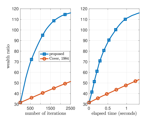
Figure 1: Wealth yielded by different algorithms on the NYSE data.

We compare the convergence speeds of Cover’s algorithm and the exponentiated gradient method with Armijo line search, for the New York Stock Exchange (NYSE) data during January 1st, 1985–June 30th, 2010 [30]. The corresponding dimensions are $n=6431$ and $d=23$. We set $\overline{\alpha}=10$, $r=0.5$, and $\tau=0.8$ for the Armijo line search procedure. The numerical experiment was done in MATLAB R2018a, on a MacBook Pro with an Intel Core i7 2.8GHz processor and 16GB DDR3 memory.

The numerical result is presented in Figure 1, where we plot the total wealth yielded by the algorithm iterates, with an initial wealth of one dollar. The proposed approach—exponentiated gradient method with Armijo line search—was obviously faster than Cover’s algorithm. For example, fixing the budget of the computation time to be one second, the proposed approach yields more than twice of the wealth yielded by Cover’s algorithm.

6.2 Quantum State Tomography

Quantum state tomography (QST) is the task of estimating the state of qubits (quantum bits), given measurement outcomes. Numerically, QST corresponds to solving a convex optimization problem specified in Example 1. Recall that in the introduction, we have shown that the corresponding objective function, $f_{\text{QST}}$, does not satisfy the bounded gradient condition and is not smooth relative to the von Neumann entropy, while mirror descent with the Burg entropy has high per-iteration computational complexity.

The following proposition is a matrix analogue to Proposition 3. A proof is provided in Section E.

Proposition 4

The function $f_{\text{QST}}$ is locally smooth relative to the von Neumann entropy on the constraint set $\mathcal{D}$. _□

Therefore, the (matrix) exponentiated gradient method—mirror descent with the von Neumann entropy—with Armijo line search is guaranteed to converge, by Theorem 1. The corresponding iteration rule has a closed-form expression [11, 40]:

$$x(\alpha)=c^{-1}\exp(\log(x)-\alpha\nabla f(x)),$$

for every $x\in\tilde{\mathcal{X}}$ and $\alpha\geq 0$, where $c$ is a positive real normalizing the trace of $x(\alpha)$. The functions $\exp$ and $\log$ denote matrix exponential and logarithm, respectively.

We test the empirical performance of the exponentiated gradinet method with Armijo line search, on real experimental data generated following the setting in [19]. We compare it with the performances of the diluted $R\rho R$ algorithm [42], SCOPT [39], and the modified Frank-Wolfe algorithm studied in [35]. We also consider the $R\rho R$ algorithm [23]; it does not always converge [42], but is typically much faster than the diluted $R\rho R$ algorithm in practice.

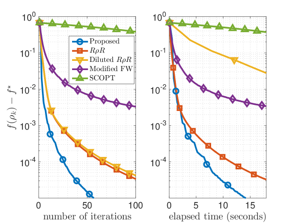
Figure 2: The 6-qubit case.

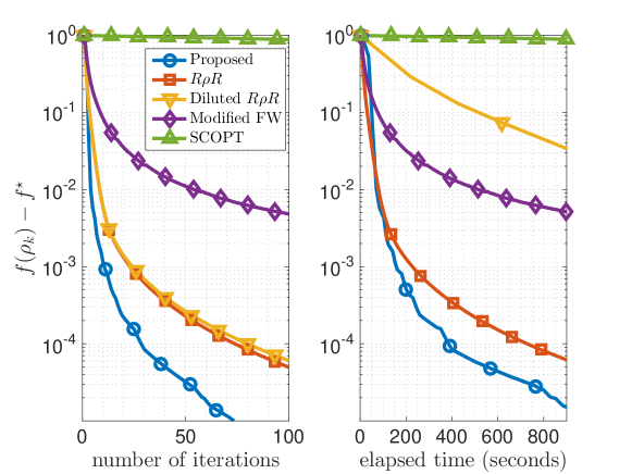
Figure 3: The 8-qubit case.

We compare the convergence speeds for the $6$-qubit ($d=2^{6}$) and $8$-qubit ($d=2^{8}$) cases, in Fig. 2 and 3, respectively. The corresponding “sample sizes” (number of summands in $f_{\text{QST}}$) are $n=60640$ and $n=460938$, respectively. The numerical experiments were done in MATLAB R2015b, on a MacBook Pro with an Intel Core i7 2.8GHz processor and 16GB DDR3 memory. We set $\alpha=10$, and $\gamma=\tau=0.5$ in Algorithm 1 for both cases. In both figures, $f^{\star}$ denotes the minimum value of $f_{\text{QST}}$ found by the five algorithms in 120 iterations.

One can observe that the exponentiated gradient method with Armijo line search is the fastest, in terms of the actual elapsed time. The slowness of the other algorithms is explainable.

1. The diluted $R\rho R$ algorithm, using the notation of this paper, iterates as

   $$x_{k+1}=c_{k}^{-1}\left[I+\beta_{k}f^{\prime}(x_{k})\right]^{\mathrm{H}}\rho_{k}\left[I+\beta_{k}f^{\prime}(x_{k})\right],$$

   where $c_{k}$ normalizes the trace of $x_{k+1}$. To guarantee convergence, the step sizes $\beta_{k}$ are computed by exact line search. The exact line search procedure renders the algorithm slow.

2. SCOPT is a projected gradient method for minimizing self-concordant functions [33, 34]. Notice that projection onto $\mathcal{D}$ typically results in a low-rank output; hence, it is possible that $\operatorname{\mathrm{Tr}}(M_{i}x_{k})=0$ for some low-rank $M_{i}$ and iterate $x_{k}$, but then $x_{k}$ is not a feasible solution because $\log(0)$ is not defined. This is called the stalling problem in [27]. Luckily, self-concordance of $f_{\text{QST}}$ ensures that if an iterate $x_{k}$ lies in $\operatorname{\mathrm{dom}}f_{\text{QST}}$, and the next iterate $x_{k+1}$ lies in a small enough Dikin ellipsoid centered at $x_{k}$, then $x_{k+1}$ also lies in $\operatorname{\mathrm{dom}}f_{\text{QST}}$. It is easily checked that $f_{\text{QST}}$ is a self-concordant function of parameter $2\sqrt{n}$. Following the theory in [33, 34], the radius of the Dikin ellipsoid shrinks at the rate $O(n^{-1/2})$, so SCOPT becomes slow when $n$ is large.

3. The Frank-Wolfe algorithm suffers for a sub-linear convergence rate when the solution is near an extreme point of the constraint set (see, e.g., [29] for an illustration in the vector case). Notice that the set of extreme points of $\mathcal{D}$ is the set of single-rank positive semi-definite matrices of unit trace. In the experimental data we have, the density matrix to be estimated is indeed close to a single-rank matrix (which is called a pure state in quantum mechanics). Therefore, the ML estimate—the minimizer of $f_{\text{QST}}$ on $\mathcal{D}$—is expected to be also close to a single-rank matrix.

Notice that the empirical convergence rate of the exponentiated gradient method with Armijo line search is linear.

Appendix A Proof of Proposition 1

Consider the two-dimensional case, where $x=(x_{i,j})_{1\leq i,j\leq 2}\in\mathbb{C}^{2\times 2}$. Define $e_{1}:=(1,0)$ and $e_{2}:=(0,1)$. Suppose that there are only two summands, with $M_{1}=e_{1}\otimes e_{1}$ and $M_{2}=e_{2}\otimes e_{2}$. Then we have $f(x)=-\log(x_{1,1})-\log(x_{2,2})$. It suffices to disprove all properties on the set of diagonal density matrices. Hence, we will focus on the function $g(x,y):=-\log x-\log y$, defined for any $(x,y)$ in the probability simplex $\mathcal{P}\subset\mathbb{R}^{2}$.

As either $x$ or $y$ can be arbitrarily close to zero, it is easily checked that the gradient of $g$ is unbounded. Now we check the relative smoothness condition. As we only consider diagonal matrices, it suffices to check with respect to the (negative) Shannon entropy:

$$h(x,y):=-x\log x-y\log y+x+y\,,\quad\forall(x,y)\in\mathcal{P}\,,$$

for which the convention $0\log 0:=0$ is adopted.

Lemma 5 ([31])

The function $g$ is $L$-smooth relative to the Shannon entropy for some $L>0$, if and only if $-Lh-g$ is convex. _□

Therefore, we check the positive semi-definiteness of the Hessian of $-Lh-g$. A necessary condition for the Hessian to be positive semi-definite is that

$$-L\frac{\partial^{2}h}{\partial x^{2}}(x,y)-\frac{\partial^{2}g}{\partial x^{2}}(x,y)=\frac{L}{x}-\frac{1}{x^{2}}\geq 0,$$

for all $x\in(0,1)$, but the inequality cannot hold for $x<(1/L)$, for any fixed $L>0$.

Appendix B Proof of Lemma 1

(Statement 2 $\Rightarrow$ Statement 1) Let $x\in\mathcal{X}\cap\operatorname{\mathrm{dom}}f$, and $z_{1},z_{2}\in\mathcal{B}_{\varepsilon_{x}}(x)\cap\tilde{\mathcal{X}}$. Define, for every $\tau\in[0,1]$, $z_{\tau}:=z_{1}+\tau(z_{2}-z_{1})$. We write

$$f(z_{2})-\left[f(z_{1})+\braket{\nabla f(z_{1}),z_{2}-z_{1}}\right] =\int_{0}^{1}\braket{\nabla f(z_{\tau})-\nabla f(z_{1}),z_{2}-z_{1}}\,\mathrm{d}\tau$$

$$\leq\int_{0}^{1}\|\nabla f(z_{\tau})-\nabla f(z_{1})\|_{2}\|z_{2}-z_{1}\|_{2}\,\mathrm{d}\tau$$

$$\leq\int_{0}^{1}L_{x}\tau\|z_{2}-z_{1}\|_{2}^{2}\,\mathrm{d}\tau$$

$$=\frac{L_{x}}{2}\|z_{2}-z_{1}\|_{2}^{2},$$

where we have applied the Cauchy-Schwarz inequality for the first inequality, and the local smoothness condition for the second inequality. Note that $\mathcal{B}_{\varepsilon_{x}}\cap\tilde{\mathcal{X}}$ is the intersection of convex sets, and hence is convex; therefore, $z_{\tau}\in\mathcal{B}_{\varepsilon_{x}}\cap\tilde{\mathcal{X}}$ for every $\tau\in[0,1]$.

(Statement 1 $\Rightarrow$ Statement 2) Let $x\in\mathcal{X}\cap\operatorname{\mathrm{dom}}f$, and $z_{1},z_{2}\in\mathcal{B}_{\varepsilon_{x}}(x)\cap\tilde{\mathcal{X}}$. Define $\varphi(z):=f(z)-\braket{\nabla f(z_{1}),z}$. Then $\nabla\varphi$ is locally Lipschitz on $\tilde{\mathcal{X}}$; moreover, since $\nabla\varphi(z_{1})=0$, the point $z_{1}$ is a global minimizer of $\varphi$. Therefore, we obtain

$$\varphi(z_{1})\leq\varphi(z_{2}-\frac{1}{L_{x}}\nabla\varphi(z_{2}))\leq\varphi(z_{2})-\frac{1}{2L_{x}}\|\nabla\varphi(z_{2})\|^{2};$$

that is,

$$f(z_{2})\geq f(z_{1})+\braket{\nabla f(z_{1}),z_{2}-z_{1}}+\frac{1}{2L_{x}}\|\nabla f(z_{2})-\nabla f(z_{1})\|_{2}^{2}.$$

Similarly, we get

$$f(z_{1})\geq f(z_{2})+\braket{\nabla f(z_{2}),z_{1}-z_{2}}+\frac{1}{2L_{x}}\|\nabla f(z_{1})-\nabla f(z_{2})\|_{2}^{2}.$$

Summing up the two inequalities; we obtain

$$\braket{\nabla f(z_{2})-\nabla f(z_{1}),z_{2}-z_{1}}\geq\frac{1}{L_{x}}\|\nabla f(z_{2})-\nabla f(z_{1})\|_{2}^{2}.$$

This implies, by the Cauchy-Schwarz inequality,

$$\|\nabla f(z_{2})-\nabla f(z_{1})\|_{2}\leq L_{x}\|z_{2}-z_{1}\|_{2}.$$

Appendix C Auxiliary Technical Lemmas for Proving Theorem 1

Lemma 6

If $x(\alpha)=x$ for some $x\in\tilde{\mathcal{X}}$, then $x$ is a solution to (P). If a point $x\in\tilde{\mathcal{X}}$ is a solution to (P), then $x(\alpha)=x$ for all $\alpha\in[0,+\infty)$. _□

Proof

That $x$ is a solution to (P) is equivalent to the optimality condition

$$\braket{\nabla f(x),z-x}\geq 0,\quad\forall z\in\mathcal{X}.$$

We can equivalently write

$$\braket{\alpha\nabla f(x)+\nabla h(x)-\nabla h(x),z-x}\geq 0,\quad\forall z\in\mathcal{X},$$

which is the optimality condition of

$$x(\alpha)=\operatorname*{\arg\min}_{z}\set{\alpha\braket{\nabla f(x),z-x}+D_{h}(z,x)}{z\in\mathcal{X}}.$$

_■

Lemma 7

For every $x\in\tilde{\mathcal{X}}$ and $\alpha>0$, it holds that

$$\braket{\nabla f(x(\alpha)),x(\alpha)-x}\leq-\alpha^{-1}D(x(\alpha),x)\leq 0.$$

_□

Proof

By definition, we have

$$\alpha\braket{\nabla f(x(\alpha)),x(\alpha)-x}+D(x(\alpha),x)\leq\alpha\braket{\nabla f(x,x-x}+D(x,x)=0.$$

_■

Corollary 2

The sequence $\set{x_{k}}$ is non-increasing. _□

Proof

The Armijo rule and Lemma 7 guarantee that

$$f(x_{k})\leq f(x_{k-1})+\tau\braket{\nabla f(x_{k-1}),x_{k}-x_{k-1}}\leq f(x_{k-1}).$$

_■

Appendix D Proof of Theorem 2

For every $u\in\mathcal{X}\cap\operatorname{\mathrm{dom}}f$, we write

$$f(x_{k-1})-f(u) \leq-\braket{\nabla f(x_{k-1}),u-x_{k-1}}$$

$$=-\braket{\nabla f(x_{k-1}),u-x_{k}}-\braket{\nabla f(x_{k-1}),x_{k}-x_{k-1}}.$$

The optimality condition for $x_{k}$ implies

$$\braket{\alpha_{k}\nabla f(x_{k-1})+\nabla h(x_{k})-\nabla h(x_{k-1}),u-x_{k}}\geq 0.$$

Applying the three-point identity [13], we obtain

$$\braket{\nabla f(x_{k-1}),u-x_{k}} \geq-\alpha_{k}^{-1}\braket{\nabla h(x_{k})-\nabla h(x_{k-1}),u-x_{k}}$$

$$=-\alpha_{k}^{-1}\left[D_{h}(u,x_{k-1})-D_{h}(u,x_{k})-D_{h}(x_{k},x_{k-1})\right]$$

$$\geq-\alpha_{k}^{-1}\left[D_{h}(u,x_{k-1})-D_{h}(u,x_{k}))\right].$$

Then we can write

$$\alpha_{k}\left[f(x_{k-1})-f(u)\right] \leq\left[D_{h}(u,x_{k-1})-D_{h}(u,x_{k}))\right]-\alpha_{k}\braket{\nabla f(x_{k-1}),x_{k}-x_{k-1}}.$$

Summing up the inequality for all $1\leq k\leq n$, we get

$$-S_{n}f(u)+\sum_{k=1}^{n}\alpha_{k}f(x_{k-1})\leq D(u,x_{0})-\sum_{k=1}^{n}\alpha_{k}\braket{\nabla f(x_{k-1}),x_{k}-x_{k-1}},$$

where $S_{n}:=\sum_{k=1}^{n}\alpha_{k}$. Corollary 2 says that the sequence $(f(x_{k}))_{k\in\mathbb{N}}$ is non-increasing; then we have

$$\sum_{k=1}^{n}\alpha_{k}f(x_{k-1})\geq\sum_{k=1}^{n}\alpha_{k}f(x_{n})=S_{n}f(x_{n}).$$

Therefore, we obtain

$$f(x_{n})-f(u)\leq S_{n}^{-1}\left[D(u,x_{0})-\sum_{k=1}^{n}\alpha_{k}\braket{\nabla f(x_{k-1}),x_{k}-x_{k-1}}\right].$$

Note that by the Armijo rule, we have

$$f(x_{0})-f^{\star} \geq\lim_{k\to\infty}f(x_{0})-f(x_{k})$$

$$=\sum_{j=1}^{\infty}\left[f(x_{j-1})-f(x_{j})\right]$$

$$\geq-\tau\sum_{j=1}^{\infty}\braket{\nabla f(x_{j-1}),x_{j}-x_{j-1}}.$$

Therefore, $\braket{\nabla f(x_{k-1}),x_{k}-x_{k-1}}$, which are non-negative by Lemma 4, must converge to zero. Theorem 2 then follows from the following lemma.

Lemma 8 ([37])

Let $\set{a_{k}}$ be a sequence of real numbers, and $\set{b_{k}}$ be a sequence of positive real numbers. Define $c_{n}:=\sigma_{n}^{-1}\sum_{k=1}^{n}b_{k}a_{k}$ for every $n\in\mathbb{N}$, where $\sigma_{n}:=\sum_{k=1}^{n}b_{k}$. If $a_{k}\to 0$ and $\sigma_{n}\to+\infty$, then $c_{n}\to 0$. _□

Appendix E Proof of Proposition 4

Note that $\operatorname{\mathrm{dom}}(f_{\text{QST}})$ is open, and hence $\operatorname{\mathrm{dom}}(f_{\text{QST}})\cap\mathcal{X}$ is relatively open in $\mathcal{X}$. It is easily checked that $f_{\text{QST}}$ is twice continuously differentiable on $\operatorname{\mathrm{dom}}(f_{\text{QST}})$, and hence on $\operatorname{\mathrm{dom}}(f_{\text{QST}})\cap\mathcal{X}$. By Proposition 2, the function $f_{\text{QST}}$ is locally smooth relative to $h(\cdot):=(1/2)\|\cdot\|_{\text{F}}^{2}$, where $\|\cdot\|_{\text{F}}$ denotes the Frobenius norm. By the quantum version of Pinsker’s inequality [21], the von Neumann entropy is strongly convex on $\mathcal{D}$ with respect to the trace norm. As all norms on a finite-dimensional space are equivalent, the proposition follows.

References

- [1] Armijo, L. Minimization of functions having Lipschitz continuous first partial derivatives. Pac. J. Math. 16, 1 (1966), 1–3.
- [2] Auslender, A., and Teboulle, M. Interior gradient and proximal methods for convex and conic optimization. SIAM J. Optim. 16, 3 (2006), 697–725.
- [3] Bauschke, H. H., Bolte, J., and Teboulle, M. A descent lemma beyond Lipschitz gradient continuity: first-order methods revisited and applications. Math. Oper. Res. 42, 2 (2017), 330–348.
- [4] Bauschke, H. H., Borwein, J. M., and Combettes, P. L. Essential smoothness, essential strict convexity, and Legendre functions in Banach spaces. Commun. Contemp. Math. 3, 4 (2001), 615–647.
- [5] Bauschke, H. H., and Combettes, P. L. Convex analysis and monotone operator thoery in Hilbert spaces. Springer, New York, NY, 2011.
- [6] Beck, A., and Teboulle, M. Mirror descent and nonlinear projected subgradient methods for convex optimization. Oper. Res. Lett. 31 (2003), 167–175.
- [7] Bertero, M., Boccacci, P., Desiderà, G., and Vicidomini, G. Image deblurring with Poisson data: from cells to galaxies. Inverse Probl. 25 (2009).
- [8] Bertsekas, D. P. On the Goldstein-Levitin-Polyak gradient projection method. IEEE Trans. Automat. Contr. AC-21, 2 (1976), 174–184.
- [9] Bonettini, S., Loris, I., Porta, F., and Prato, M. Variable metric inexact line-search-based methods for nonsmooth optimization. SIAM J. Optim. 26, 2 (2016), 891–921.
- [10] Bonettini, S., Zanella, R., and Zanni, L. A scaled gradient projection method for constrained image deblurring. Inverse Probl. 25 (2009).
- [11] Bubeck, S. Convex optimization: Algorithms and complexity. Found. Trends Mach. Learn. 8, 3–4 (2015), 231–358.
- [12] Byrne, C., and Censor, Y. Proximity function minimization using multiple Bregman projections, with application to split feasibility and Kullback-Leibler distance minimization. Ann. Oper. Res. 105 (2001), 77–98.
- [13] Chen, G., and Teboulle, M. Convergence analysis of a proximal-like minimization algorithm using Bregman functions. SIAM J. Optim. 3, 3 (Aug. 1993), 538–543.
- [14] Cover, T. M. An algorithm for maximizing expected log investment return. IEEE Trans. Inf. Theory IT-30, 2 (1984), 369–373.
- [15] Cover, T. M. Universal portfolios. Math. Finance 1, 1 (1991), 1–29.
- [16] Cover, T. M., and Ordentlich, E. Universal portfolios with side information. IEEE Trans. Inf. Theory 42, 2 (1996), 348–363.
- [17] Csiszár, I., and Körner, J. Information Theory: Coding Theorems for Discrete Memoryless Systems, second ed. Cambridge Univ. Press, Cambridge, UK, 2011.
- [18] Csiszár, I., and Tusnády, G. Information geometry and alternating minimization procedures. Stat. Decis., Supplement 1 (1984), 205–237.
- [19] Häffner, H., Hänsel, W., Roos, C. F., Benhelm, J., Check-al-kar, D., Chwalla, M., Körber, T., Rapol, U. D., Riebe, M., Schmidt, P. O., Becher, C., Gühne, O., Dür, W., and Blatt, R. Scalable multiparticle entanglement of trapped ions. Nature 438 (2005), 643–646.
- [20] Hazan, E., and Kale, S. An online portfolio selection algorithm with regret logarithmic in price variation. Math. Finance 25, 2 (2015), 288–310.
- [21] Hiai, F., Ohya, M., and Tsukada, M. Sufficiency, KMS condition and relative entropy in von Neumann algebras. Pac. J. Math. 96, 1 (1981), 99–109.
- [22] Hiriart-Urruty, J.-B., Strodiot, J.-J., and Nguyen, V. H. Generalized Hessian matrix and second-order optimality conditions for problem with data. Appl. Math. Optim. 11 (1984), 43–56.
- [23] Hradil, Z. Quantum-state estimation. Phys. Rev. A 55, 3 (1997).
- [24] Ioffe, A., and Milosz, T. On a characterization of functions. Cybern. Syst. Anal. 38, 3 (2002), 313–322.
- [25] Juditsky, A., and Nemirovski, A. First-order methods for nonsmooth convex large-scale optimization, I: General purpose methods. In Optimization for Machine Learning, S. Sra, S. Nowozin, and S. J. Wright, Eds. MIT Press, Cambridge, MA, 2012, ch. 5.
- [26] Kivinen, J., and Warmuth, M. K. Exponentiated gradient versus gradient descent for linear predictors. Inf. Comput. 132 (1997), 1–63.
- [27] Knee, G. C., Bolduc, E., Leach, J., and Gauger, E. M. Maximum-likelihood quantum process tomography via projected gradient descent. arXiv:1803.10062v1.
- [28] Kulis, B., Sustik, M. A., and Dhillon, I. S. Low-rank kernel learning with Bregman matrix divergences. J. Mach. Learn. Res. 10 (2009), 341–376.
- [29] Lacoste-Julien, S., and Jaggi, M. On the global linear convergence of Frank-Wolfe optimization variants. In Adv. Neural Information Processing Systems 28 (2015).
- [30] Li, B., Sahoo, D., and Hoi, S. C. H. OLPS: A toolbox for on-line portfolio selection. J. Mach. Learn. Res. 17 (2016), 1–5.
- [31] Lu, H., Freund, R. M., and Nesterov, Y. Relatively smooth convex optimization by first-order methods, and applications. SIAM J. Optim. 28, 1 (2018), 333–354.
- [32] Nemirovsky, A. S., and Yudin, D. B. Problem Complexity and Method Efficiency in Optimization. John Wiley & Sons, Chichester, 1983.
- [33] Nesterov, Y. Introductory Lectures on Convex Optimization. Kluwer, Boston, MA, 2004.
- [34] Nesterov, Y., and Nemirovskii, A. Interior-Point Polynomial Algorithms in Convex Programming. SIAM, Philadelphia, PA, 1994.
- [35] Odor, G., Li, Y.-H., Yurtsever, A., Hsieh, Y.-P., El Halabi, M., Tran-Dinh, Q., and Cevher, V. Frank-Wolfe works for non-Lipschitz continuous gradient objectives: Scalable Poisson phase retrieval. In IEEE Int. Conf. Acoustics, Speech and Signal Processing (2016), pp. 6230–6234.
- [36] Paris, M., and Řeháček, J., Eds. Quantum State Estimation. Springer, Berlin, 2004.
- [37] Polyak, B. T. Introduction to Optimization. Optimization Softw., Inc., New York, NY, 1987.
- [38] Rockafellar, R. T., and Wets, R. J. Variational Analysis. Springer, Berlin, 2009.
- [39] Tran-Dinh, Q., Kyrillidis, A., and Cevher, V. Composite self-concordant minimization. J. Mach. Learn. Res. 16 (2015), 371–416.
- [40] Tsuda, K., Rätsch, G., and Warmuth, M. K. Matrix exponentiated gradient updates for on-line learning and Bregman projection. J. Mach. Learn. Res. 6 (2005), 995–1018.
- [41] Vardi, Y., Shepp, L. A., and Kaufman, L. A statistical model for positron emission tomography. J. Am. Stat. Assoc. 80, 389 (1985), 8–20.
- [42] Řeháček, J., Hradil, Z., Knill, E., and Lvovsky, A. I. Diluted maximum-likelihood algorithm for quantum tomography. Phys. Rev. A 75 (2007).