Conjoining uncooperative societies
   facilitates evolution of cooperation

Abstract

Social structure affects the emergence and maintenance of cooperation. Here we study the evolutionary dynamics of cooperation in fragmented societies, and show that conjoining segregated cooperation-inhibiting groups, if done properly, rescues the fate of collective cooperation. We highlight the essential role of inter-group ties, that sew the patches of the social network together and facilitate cooperation. We point out several examples of this phenomenon in actual settings. We explore random and non-random graphs, as well as empirical networks. In many cases we find a marked reduction of the critical benefit-to-cost ratio needed for sustaining cooperation. Our finding gives hope that the increasing worldwide connectivity, if managed properly, can promote global cooperation.

1 Introduction

A core problem in evolutionary game theory is that of cooperation. Cooperation involves individuals paying a cost to benefit others, and is a ubiquitous feature of the social life [1, 2]. The structure of social networks affect pathways of information, exchange, and other interpersonal mechanisms which undergird cooperation [2]. Thus a natural question in the mathematical study of evolutionary dynamics of cooperation is how network structure influences collective cooperative outcomes [5, 6, 7, 8, 1].

Here we look at the evolution of cooperation from a new perspective. We ask the question of how the interconnection between segregated groups can promote cooperation. Similar to individuals forming groups towards collective individually-implausible accomplishments, sometimes groups come together to form larger composite structures. Examples abound throughout history, from trade and intermarriage relations between tribes and communities in antiquity, to the waves of globalization which increasingly connect local entities for economic, cultural, and technological exchange. Another example is project management at different levels in corporations and organizations, which involves the cooperative division of labor between sparsely-interconnected distinctly-specialized units.

We use the framework of evolutionary graph theory [6, 7, 1] to study settings where groups that are individually undesirable for cooperation can be conjoined to build larger cooperation-promoting structures. We first study the conjoining of cohesive communities (clique-like structurally-homogeneous groups) under different connection schemes. We then focus on extremely-heterogeneous structures. We study stars and their various interconnection schemes, as well as rich clubs, and introduce ensuing topologies that are super-promoters of cooperation. Then we focus on bipartite graphs. In addition to these ideal graph families, we consider several random graph models. Finally, we consider empirical social networks and investigate the role of community structure on the evolution of cooperation. The findings are consistent across topologies: sparse interconnections of cooperation-inhibiting graphs leads to composite structures that are better for the evolution of cooperation.

Under the framework of mathematical graph theory, social structure is described by a graph, in which nodes represent individuals and links represent interactions and/or relations. In the simplest setting, individuals are conventionally envisaged with two possible strategies pertaining to a $2\times 2$ context-specific payoff matrix which characterizes their interaction. The outcomes of these interactions (‘games’) determine the ‘fitness’ values of the individuals: those who accrue more benefits are endowed with higher fitness, which governs their influence over the peers’ choices of strategy. The most stringent form of cooperation is found in the Prisoner’s Dilemma (PD) game, in which individuals are either cooperators (paying a cost $c$ and bestowing benefit $b>c$ upon the interaction partner) or defectors (who seek to benefit without paying a cost). The analysis throughout this paper uses the so-called ‘donation game’ version of PD (as shall be discussed, generalization to arbitrary symmetric 2-player games is straightforward). In this game, mutual cooperation has payoff $b-c$, unilateral cooperation has payoff $-c$ for the cooperator and $b$ for the defector, and mutual defection has payoff 0. The ratio ${b}/{c}$ characterizes the trade-off players face. Throughout this paper, without loss of generality, we set $c=1$. This is simply equivalent to a change of scale in payoffs, and helps brevity of notation. The strategies of the agents change according to death-birth (dB) updating: a random individual is chosen to update; it adopts one of the the neighbors’ strategies proportional to payoff. The small ‘d’ indicates that death is random, while the large ‘B’ indicates that birth is under selection. The probability that the chosen node copies the strategy of neighbor $y$ is proportional to ${1+\delta\pi_{y}}$, where $\delta$ denotes the selection strength and $\pi_{y}$ is the average payoff that node $y$ gleans playing with its own neighbors. We consider the limit of weak selection. To see if natural selection favors or hinders collective cooperation, we must calculate the probability that a single cooperator emerging at a random place in the network takes over the population. Natural selection favors cooperation if this fixation probability exceeds that of the fixation probability of a defector. Otherwise, natural selection inhibits cooperation.

Before we proceed, we point out a central feature of network models of cooperation, such as ours. In these models, social influence spreads beyond immediate neighbors. In conventional models of social contagion, such as simple contagion models, which often describe information diffusion, and complex contagion models, which often describe spread of behaviors [11, 12], the ego’s activation probability depends on the states of the alters. An activated alter exerts the same influence on the ego regardless of the states of the neighbors of that alter. For example, in the simple-contagion model of information diffusion, the ego needs to have heard the news from only one alter to have become informed, and is agnostic to how many neighbors of that alter have heard the news. Or in threshold models of complex contagion, the ego is activated once a certain number or fraction of alters are activated, regardless of the ego’s second neighbors. In contrast, due to the strategic nature of cooperative dynamics, in our model, the radius of influence is two [13]. Ego is influenced directly by the strategies of the alters (from whom ego copies its strategy), and also indirectly by those of the neighbors of each alter (who contribute to the payoff of that alter). Our model, with a setting similar to the previous theoretical [5, 6, 7, 1] and experimental [3, 4] studies of human cooperation, thereby adds a strategic element to pure imitation dynamics. Our model shares one similarity with simple contagion processes: having one alter who has adopted each of the strategies makes the ego’s adoption probability for that strategy nonzero.

A recently-discovered formulation gives the exact condition under which natural selection favors cooperation on a given network [1]. The solution utilizes the mathematical equivalence of the problem to that of coalescing random walks on the graph, and the solution is in terms of the remeeting times of random walkers initiated at each node. In the Methods section, we provide a brief overview of the framework. For a given network, the framework produces a quantity (which we denote by $b^{*}$) that determines the fate of cooperation. For any network, we have $|b^{*}|>1$. If $b^{*}$ is positive, then $b^{*}$ is the critical benefit-to-cost ratio. That is, natural selection favors the fixation of cooperation over that of defection on the given network if the benefit-to-cost-ratio is greater than $b^{*}$. The closer $b^{*}$ is to unity, the better the network is for promoting cooperation. Conversely, if $b^{*}$ is negative, natural selection inhibits cooperation for any benefit-to-cost ratio. In these cases, the network promotes ‘spite’ instead of cooperation. That is, individuals are willing to pay a cost to reduce the payoff of others. The closer the value of $b^{*}$ is to $-1$, the more strongly the network promotes spite. The convention of the literature has hitherto been using $b^{*}$ to characterize the conduciveness of networks for cooperation [6, 7, 1, 4, 1]. In the SI, we remark that $1/b^{*}$ can also be used, we discuss the advantages of each measure, and we find that some of the numerical results are visually better presentable using $1/b^{*}$ instead of $b^{*}$. For consistency with the previous literature, we use $b^{*}$ to present the results in the main text.

We consider distinct settings in which structures that are known to inhibit cooperation can be connected under various schemes to create larger structures that promote cooperation. In the main text, for brevity, we only provide the simplified version of the results in the large-$n$ limit (that is, the leading term), and present the full expressions in the corresponding Supplementary material. We use the terminology of asymptotic analysis throughout. We say $b^{*}$ grows as $an^{b}$, denoted $b^{*}\sim an^{b}$, if $\lim_{n\to\infty}b^{*}/(an^{b})=1$. Equivalently, we call $an^{b}$ the leading term of $b^{*}$.

2 Cohesive communities

Suppose there is a complete graph (clique) of $n$ nodes. For a clique, selection does not favor cooperation, regardless of $b$. Namely, the value of $b^{*}$ that the method gives is negative. This means that cliques promote spite.

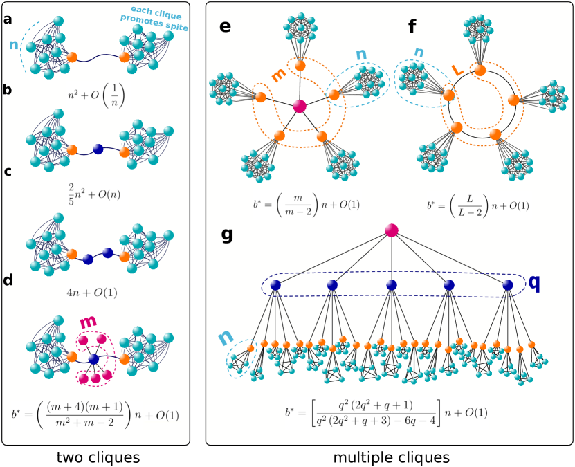
Figure 1: From spite to cooperation by conjoining cliques. Cohesive communities (cliques) hinder the flourishing of cooperation. Each clique promotes spiteful behavior. Conjoining cliques to build larger networks facilitates cooperation. This figure illustrates several topologies of conjoining two (a-d) or multiple (e-g) cliques to build composite cooperation-promoting structures. If we connect two cliques, either directly (a) or via an intermediary node (b), then the composite structure is a promoter of cooperation: the critical benefit-to-cost ratio, $b^{*}$, grows with the square of the clique size, $n^{2}$. This is a steep increase of $b^{*}$ with network size, thus although cooperation is in principle possible, it might be impractical for actual settings. (c) Having two intermediary nodes leads to further improvement: the critical benefit-to-cost ratio now grows linearly with $n$. This is a much slower increase of $b^{*}$ with network size, as compared to the previous case. Thus, this is a more desirable interconnection scheme for actual scenarios. (d) The broker node who bridges two cliques can also be connected to leaf nodes. In this case, too, $b^{*}$ grows linearly with $n$. The following conjoining schemes for multiple cliques produce composite structures that promote cooperation with a critical benefit-to-cost ratio, $b^{*}$, that grows linearly with the size of individual cliques. (e) A broker node connects multiple cliques. (f) A ring of cliques which represents the ‘caveman graph’. (g) Hierarchical organization of cliques.

In real-world networks, communities can join together to form larger structures that are better for cooperation. Suppose there are two cliques (which for simplicity we consider to be of the same size, and the analytical steps for the general case are the same) and we connect a node from the first one to a node in the second one (Fig. 1a). We call these two nodes ‘gate nodes’, and the rest of the nodes in the two communities ‘commoners’. In organizational settings, for example, these gate nodes are called ‘boundary spanners’. They are essential for intergroup flow of information and ideas, intergroup coordination and collaboration, and organizational effectiveness and novelty [14]. For two communities of size $n$ with the described interconnection, $b^{*}$ is positive and finite, but it grows as ${1\times n^{2}}$. Thus it is in principle possible that natural selection favors cooperation, but the necessary $b^{*}$ grows quickly with network size. This might be infeasible for actual settings. Connecting the gate nodes via an intermediary ‘broker’ node (Fig. 1b) reduces the leading term to ${(2/5)\times n^{2}}$, which is slightly better, but it still grows quickly with $n$. Marked reduction of $b^{*}$ ensues if instead of one broker, there are two brokers on the path between the gate nodes (Fig. 1c). Each group is connected to a third-party trustee node, or representative, and exchange is done via these two nodes. With two broker nodes in the middle, then the leading term of $b^{*}$ drops to $4n$, thus $b^{*}$ grows considerably slower with network size. This interconnection scheme offers a substantial improvement and the two communities which individually promote spite can now be conjoined to form a new composite network which supports cooperation with more plausible values of $b^{*}$.

Longer chains of intermediary nodes between the two cliques is mathematically possible, but relatively less common in actual settings. The possible exceptions are chain-of-command structures which resemble this topology: a group of decision-makers sit at one end (the first clique) and through a chain of intermediary units, the agenda reaches the bottom-most unit (the second clique) which is in charge of implementation. For chains with more than two intermediary nodes, the analytical results become too lengthy to be presented. But fortunately the employed coalescing random walks framework enables numerical extraction of the leading term. If the chain of intermediaries has length $L$, with $L\ll n$, then the leading term of $b^{*}$ drops further to ${n\times 4/(L-1)}$. The results for intermediate values of $L$, with the possibility of $L>n$, are presented in the SI.

There are also alternative intercommunity connection schemes that offer a marked reduction in $b^{*}$. For example, if there is one broker node between the gate nodes, and the broker is connected to $m>1$ peripheral leaf nodes (Fig. 1d), then the leading term of $b^{*}$ is given by ${n(m+2)(m+5)/[m(m+3)]}$, which is linear in $n$.

In actual settings, often there are more than two communities (local social networks, production units, etc.). Urbanization has led to a proliferation of diverse subcultures and enhanced interaction and diffusion between them as a daily principle of contemporary life [15, 16]. In organizational settings, ‘network brokers’ can bridge existing ‘structural holes’ and connect multiple segregated sectors and facilitate cooperation among them [17, 18]. An simple example of such a setting would be a star of cliques: $m>2$ communities connected via a highly-central broker node (Fig. 1e). With this $m$-community structure, with $m>2$ communities, $b^{*}$ has the leading term $n\times m/(m-2)$. Linear growth in community size $n$ indicates a substantial improvement over a single community or two communities is attained.

Another interconnection scheme of multiple cohesive communities is the so-called ‘caveman graph’ from the sociological literature [19] (Fig. 1f). With $L>2$ cliques, situated on a ring, the leading term of $b^{*}$ is given by $n\times L/(L-2)$, which is linear in clique size.

Cliques can also be organized hierarchically, such as in modern organizational bureaucracies (Fig. 1g). In this case, too, for large cliques, the leading term of $b^{*}$ grows linearly with clique size, as shown in Fig. 1g.

3 Star-like structures

A star graph comprises a hub and $n$ leaf nodes connected to the hub. In this strictly-centralized system, natural selection does not promote cooperation regardless of $b$. Similar to the case of cliques, stars can be connected to promote collective cooperation. If we have two stars, one with $n$ leaf nodes and the other with $\alpha n$ leaf nodes (Fig. 2a), then if we connect the hubs, $b^{*}$ for large $n$ approaches a constant ${(8+\alpha+1/\alpha)/4}$. The smallest possible $b^{*}$ for two stars is $5/2$, which pertains to $\alpha=1$ (identical stars). The independence from network size is a remarkable feature that star structures exhibit.

If we connect the hubs via one intermediary broker node, we get ${b^{*}\sim(10+\alpha+1/\alpha)/4}$. For two identical stars, this simplifies to $b^{*}\sim 3$. We can also connect the hubs via a chain of $L$ intermediary brokers, such as in a chain-of-command structure with a decision-making unit at the top and and an implementation unit at the bottom. For $L\geq 1$, the leading term of $b^{*}$ is given by ${(8+2L+\alpha+1/\alpha)/(L+3)}$. In all these cases, it is remarkable that for large network size, $b^{*}$ tends to a constant. This independence from network size evinces the high merit of locally-star-like structures in the promotion of cooperation.

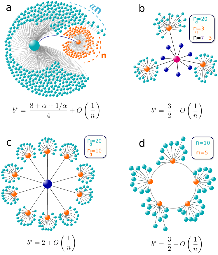
Figure 2: Super-promoters of cooperation. Star graphs represent extreme core-periphery structures where a central node is connected to many leaf nodes. Although a single star hinders cooperation, connecting stars promotes cooperation. All reported critical benefit-to-cost ratios, $b^{*}$, pertain to the limit of large population size. Exact formulas are presented in the SI, Section S2. (a) Two stars, one with $n$ leaf nodes and the other with $\alpha n$ leaf nodes. (b) An imperfect meta-star: a central node has n peripheral nodes, $n_{g}$ of them are hubs, while $n_{d}$ of them are leaves. If $n_{g}\ll n\ll n_{d}$, then $b^{*}$ tends to 3/2 and the average degree tends to 2. Thus, the structure is a super-promoter of cooperation, since $b^{*}$ is less than the average degree. (c) The perfect meta-star is a hierarchical structure with a head node connected to $n$ subsidiary nodes, each of them connected to $n_{d}$ peripheral nodes. The reported result is for the case $n\ll n_{d}$, which means most of the population belongs to the bottom layer. (d) A more flat hierarchical structure: there are $m$ head nodes connected on a ring, each with $n$ peripheral nodes. For $m\ll n$, this graph becomes a super-promoter of cooperation, outperforming the strict hierarchy.

In many actual settings, star-like structures are not directly connected as we envisaged above. Rather, global hubs are connected to local large-scale hubs, which are in turn connected to local peripheral nodes. This leads to a hierarchical organization: the head unit connects to a number of subsidiary units, each of them connect in turn to subordinate units, and so an. To study this interconnection scheme, we consider graphs with megahubs and hubs in a nested manner. We consider only two levels, though the calculation can be in principle extended to more. Out of the $n$ total leaf nodes of a star graph, we take $n_{g}$ of them and attach $n_{d}$ nodes to each (Fig. 2b). The total number of nodes will be ${1+n+n_{g}n_{d}}$, and the number of links is $n+n_{g}n_{d}$. The full expressions for $b^{*}$ are long (presented in the SI, Section S2.D), but simplifications can be obtained in some interesting limits. We consider the case where the number of leaf nodes are much larger than the number of hubs. This is the case in many actual settings, to the extent that the marked imbalance between the latter two numbers constitutes the cornerstone of many egalitarian social discourses and movements. If we have $n_{g}\ll n$, then the leading term of $b^{*}$ approaches ${3/2}$. Whether $n_{d}$ and $n$ are of the same order of magnitude, or if we have$n\ll n_{d}$, only affects the second leading order terms. This leading behavior of $b^{*}$ is particularly interesting because the average degree approaches 2 in these cases, and $b^{*}$ being less than the average degree is a rare property of graphs. Hence we can dub these structures ‘super-promoters’ of cooperation.

We can readily generalize these results to the fully-hierarchical structure (where $n_{g}=n$), that is, a star of stars (Fig. 2c). A mega-hub is connected to $n$ hubs which are each connected to $n_{d}$ leaf nodes. In the limit of $n\ll n_{d}$, $b^{*}$ approaches 2, which indicates that this structure is a strong promoter of cooperation. Full results are presented in the SI, Section S2.E.

Hierarchies can also be more ‘flat’, which is getting popular in certain management approaches [20]. The simplest model would be to have the upper layer of nodes connect horizontally instead of hierarchically. We consider the simple case where the hubs of $m$ stars, each with $n$ leaf nodes, are connected on a ring (Fig. 2d). For large $n$, the leading term of $b^{*}$ approaches ${(3m-1)/(2m-2)}$, which is independent of $n$. This means that for large $m$, the value of $b^{*}$ approaches $3/2$. The average degree in this limit approaches 2. Hence, a ring of stars is another super-promoter of cooperation. The full results for this setup are presented in the SI, Section S2.I.

4 The Rich Club

A rich-club network is one comprised of a small dense core of connection-rich high-degree nodes and a large sparse periphery. These structures are found across social and technological networks. The notion of ‘oligarchy’ in institutions and organizations is usually linked to structures that can be characterized by such a rich-club feature [21]. Other examples with this feature include the social network of company executives and directors (within-company [22], national inter-company [23], and international inter-company [24]), the collaboration network between academics [25], and the Internet [26].

As a simple example with this characteristic, we consider a clique of $n_{c}$ nodes (where $c$ denotes ‘core’) and $n_{p}$ peripheral nodes. Each core node is connected to every other core node and every peripheral node. Each peripheral node is connected to every core node but to none of the other peripheral nodes. In the special case of $n_{c}=1$, this becomes a star graph. For a single rich-club network, natural selection does not favor cooperation, regardless of $b$. Similar to the case of a single clique, single rich-club networks promote spite.

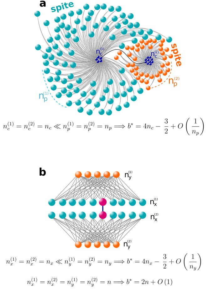
Figure 3: Rich clubs and bipartite graphs. (a) Rich-club graphs comprise a dense core and a large, sparse periphery. A single rich club hinders cooperation, but conjoined rich clubs promotes cooperation. For the simple case of two identical rich clubs, with the periphery size, $n_{p}$, much larger than the core, $n_{c}$, the critical benefit-to-cost ratio $b^{*}$ grows linearly with $n_{c}$. (b) Complete bipartite graphs comprise two distinct groups of nodes, where links exist only between the two groups, but not within each group. Examples are buyer-seller networks or heterosexual marriage networks. A single bipartite graph hinders cooperation, but connecting them promotes cooperation. For the simple case of two identical graphs, each with two groups of the same size, $b^{*}$ grows linearly with group size $n$.

To improve the situation, we connect two rich-club networks by connecting a ‘gate’ node in the first core to a gate node in the second (Fig. 3a). An actual example of conjoining rich clubs via cores is that director networks of different companies often connect, and they do so predominantly via their cores, rather than the peripheries—creating ‘interlocked directorates’ [27]. In the simple case of two identical rich-club networks with $n_{c}\ll n_{p}$ (small core and large periphery), the leading term of $b^{*}$ is given by $4n_{c}-3/2$, which is a linear function of ${n_{c}}$. That is, the leading behavior in the large-$n_{p}$ limit only depends on the number of core nodes and is independent of the number of peripheral nodes. In the case of $n_{c}=1$, this leading term is $5/2$, which is consistent with our previous findings for star graphs. For $n_{c}=2$, the leading term of $b^{*}$ is 13/2. The results point out a remarkable feature of these structures: when the periphery is large, the fate of the collective outcome is determined solely by the core.

5 Bipartite structures

In a bipartite network, nodes can be divided into two distinct groups, where there is no intra-group link. For example, traditional heterosexual marriage networks comprised two disjoint sets; males only connected to females and vice versa. Other examples include buyer/seller [28], and employer/employee [29] bipartite networks.

Here we present the results for the simplest case of a bipartite graph which is analytically tractable: we consider a complete bipartite graph. A complete bipartite network is one which has two groups, and each node is connected to every node in the other group but no node in its own group. Natural selection does not promote cooperation on a complete bipartite graph, regardless of $b$. If we connect two bipartite networks, however, the situation improves (Fig. 3b). Consider a bipartite graph comprising two groups of nodes with sizes $n_{x}$ and $n_{y}$, respectively. Suppose we connect two identical such bipartite graphs by connecting a type-$x$ node in the first graph in a type-$x$ node in the second. In the special case of $n_{x}=n_{y}=n$, $b^{*}$ grows linearly with $n$. The leading term of $b^{*}$ in this case is given by $2n$. Alternatively, if $n_{x}\ll n_{y}$, then the leading term of $b^{*}$ only depends on $n_{x}$, and is given by $4n_{x}-3/2$. Hence, similar to rich clubs, if a large group of nodes are not interconnected within themselves and are all connected only to another small group of nodes, the collective outcome will be determined by that small group.

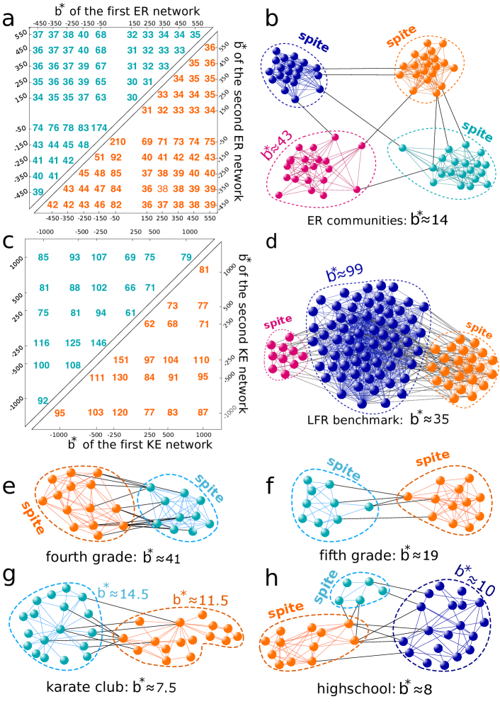
Figure 4: Conjoining random graphs and empirical networks. a) Conjoining two Erdős-Rényi random graphs directly (lower triangle) and via one broker node (upper triangle). b) Extension to more than two graphs: four ER graphs with link-formation probabilities 0.8 (top left), 0.7 (top right), 0.45 (bottom right), and 0.35 (bottom left). The inter-community link probability is 0.01. c) Conjoining two scale-free networks generated by the model of Klemm and Eguiluz [31]. d) An example network with community structure generated by the LFR benchmark [6]. Four empirical friendship networks (e-h). We employed standard community detection algorithms to partition the data set into communities, and calculated $b^{*}$ for the whole network and for each community separately. In every case, the whole network is better than individual subnetworks in promoting cooperation.

6 Random graphs and empirical social networks

Since actual social networks typically have more randomness than the ideal structured considered above, we investigate random networks to check if they have qualitatively similar properties. Our first test (discussed in the SI, Section S8) is to add structural noise to the above-considered topologies and verify that the $b^{*}$ values are indeed robust against structural deviations. For the next check, we investigate how conjoining cooperation-inhibiting random networks can promote cooperation. We generate 10 random Erdős-Rényi graphs [30], with values of $b^{*}$ that are undesirable for cooperation: negative (promoting spite) or highly positive (hindering cooperation). Network size is fixed at 40. There are 55 possible network pairs (45 pairs in which the two networks are different and 10 pairs in which they are identical), and there are 1600 ways to conjoin two networks via one gate node in each. We calculate the median value of $b^{*}$ among all these possible conjoinings for each pair of networks. The lower triangle in Fig. 4a presents the resulting $b^{*}$ of the conjoined network against the $b^{*}$ of the first and the second network. The upper triangle presents the results for the same procedure, except the gate nodes are connected via one broker node, instead of being directly connected. It can be seen that in most cases, a substantial improvement is achieved in both conjoining schemes. The most resistant case is the one with $b^{*}=-50$. Note that networks whose $b^{*}$ is negative are promoters of spite, and the closer to zero the value of $b^{*}$ is, the more strongly the structure promotes spite. The results indicate that if the spite-promotion capacity of either group is high, conjoining them would be less helpful collectively. In Fig. 4b we illustrate that the conjoining mechanism works also for more than two ER networks. In the example case shown, three of the four ER networks promote spite, and one of them promotes cooperation with $b^{*}\approx 43$. Creating inter-community links between these four groups with probability $0.01$ begets a marked improvement: the overall structure has $b^{*}\approx 14$, which is considerably better than each of the individual groups for promoting cooperation. A generalization of this procedure gives rise to the stochastic block model, which we investigate in the SI.

The same conjoining procedure is applicable to networks with heavy-tailed degree distributions, which emulate actual social networks more realistically than ER networks. Here we use the model proposed by Klemm and Eguiluz [31] to generate scale-free networks with both small-world property and high clustering coefficient, which are both ubiquitous features in social networks. The results are presented in Fig. 4c. Conjoining every pair of networks produces a composite network with positive $b^{*}$. In the SI, we present results for four additional scale-free models. The results are qualitatively similar, and the improvement in $b^{*}$ via conjoining ensues consistently.

To study the effect of community structure on the cooperative outcome, we employ the Lancichinetti-Fortunato-Radicchi (LFR) benchmark [6] that are used for comparing community-detection algorithms. The procedure generates networks with community structure in which the degree distribution within each community and the distribution of community sizes are both heavy-tailed. Fig. 4d depicts an example case with 100 nodes divided into three communities. The degree distribution is scale-free with exponent 2. The community sizes are 10, 23, and 67. Only the largest community has a positive $b^{*}$, with $b^{*}\approx 99$. The composite network (with mixing parameter 0.1) has $b^{*}\approx 35$. In Supplementary Method 1.8, we provide a systematic investigation for LFR networks and show that, consistent with the above findings, when communities are not conducive to cooperation, sparse interconnections tend to generate composite networks better than the individual modules.

We can apply the same mathematical formalism to real-world social network data. We use offline social networks that pertain to friendships, to ascertain that cooperative dynamics would be reasonable. We use two children friendship networks of fourth grade and fifth grade students [33, 34] (for the third grade, no community structure is detected because the network is dense and most people are friends with most others, so we did not use it). The second data set is the well-known friendship network of the members of a Karate club [35], and the third data set we use is Coleman’s classic highschool friendship network data set [36]. The results are presented in Fig. 4, panels e-h (more detailed results are presented in Supplementary Table 1). We divided the graphs into two communities using the Girvan-Newman method [37]. In cases where using three as the number of communities returned meaningful results, we considered both two and three communities separately. For all networks, the algorithm returned single-node communities for more than three communities, so we did not consider those cases. In all cases, the collective cooperative merit of the network is markedly better than that of the individual communities. This reaffirms the advantageousness of inter-group connection vis-à-vis cooperation.

7 Discussion

Each population structure can be quantified according to its intrinsic propensity to promote cooperation (paying a cost to benefit others) or spite (paying a cost to harm others) [1]. Here we report the observation that sparsely conjoining cooperation-inhibiting structures tend to produce cooperation-promoting structures. We have explored this effect when joining together fully connected cliques, star-like structures (which are dominated by a single individual), rich-clubs, and even random graphs. We have found the phenomenon in examples of real social networks that already consist of conjoined sub-structures.

In our findings, conjoining two graphs that are already favorable for cooperation always results in a cooperation-promoting composite structure, though sometimes the composite graph might not promote cooperation as strongly as the two individual graphs did. But we did not find any example in which the composite graph would inhibit cooperation, that is, either with $b^{*}$ significantly larger than those of the two initial graphs, or with a negative $b^{*}$. We investigated random and non-random graph families considered in this paper, and several others.

An extension to our work would be finding better conjoining schemes for cliques. Here we showed that conjoining cliques in the manners described above results in composite networks that are considerably better than individual cliques. These conjoining methods yield $b^{*}$ values that grow linearly with $n$. For very large networks, this improvement might still not be enough. A valuable extension would be to find structures that, similar to the case of stars and rich clubs, would produce $b^{*}$ that reaches a constant for large clique size.

We note that evolutionary graph theory, which we employed in this paper, is a general approach to study the effect of population structure on natural selection. It is not limited to any particular game and not restricted to one shot interactions. The results are generalizable to any matrix game (see Methods). Hence the competing strategies could instantiate repeated interactions and conditional behavior [38]. Extensions of evolutionary graph theory can be used to study direct reciprocity with crosstalk [39], and indirect reciprocity with optional interactions and private information [40]. On the other hand, there are social settings our model is not applicable to. For example, if each individual interacts with only a subset of its neighbors, then exclusion and inclusion become essential elements of network power. This is an important feature in Network Exchange Theory [41]. In this case, broker nodes have leverage over others due to the high exclusion/inclusion asymmetry. Our model does not consider the possibilities of exclusion and inclusion, and each player plays with every neighbor. Thus an interesting extension to the present paper would be to study analytically the said effects of exclusion/inclusion in a game-theoretical setting to build on the previous experimental work, particularly Network Exchange Theory.

Finally, we highlight that our results are qualitatively consistent with several simulation studies in the literature across different contexts: cooperation is promoted by interdependence between networks in spatial public goods games and the Prisoner’s Dilemma on interdependent networks [42, 43, 44], even if it is endogenous and inter-population links are only rewarded to high-payoff individuals [45]. The same is true if multiple types of interactions are considered, resulting in a multiplex network [46].

Our findings suggest a recipe for how to build societal structures that effectively promote cooperation, and together with the ensemble of previous results in the literature, they engender hope regarding the increasing interconnection of the contemporary world.

8 Methods

We follow a recently-discovered framework for unweighted, undirected graphs without self-loops [1]. Let us denote the degree of node $x$ with $k_{x}$ and its set of neighbors by $\mathcal{N}_{x}$. Then, we define $p_{x}$ as the probability that a random walk of length 2 initiated at node $x$ will terminate at node $x$:

$$p_{x}\stackrel{{\scriptstyle\text{def}}}{{=}}\,\displaystyle\frac{1}{k_{x}}\sum_{y\in\mathcal{N}_{x}}\,\displaystyle\frac{1}{k_{y}}.$$ (1)

We then solve the following system of $\binom{N}{2}$ linear equations for symmetric quantities $\tau_{xy}$, which are the meeting times of two random walkers initiated at nodes $x$ and $y$:

$$\tau_{xy}=\tau_{yx}=(1-\delta_{xy})\Bigg{[}1+\frac{1}{2k_{x}}\sum_{z\in\mathcal{N}_{x}}\tau_{zy}+\frac{1}{2k_{y}}\sum_{z\in\mathcal{N}_{y}}\tau_{zx}\Bigg{]}.$$ (2)

Here, $\delta_{xy}$ equals unity if $x=y$ and is zero otherwise. Using these quantities, we define $\tau_{x}$ for each node as the expected remeeting time of two random walkers initiated at node $x$ as follows:

$$\tau_{x}\stackrel{{\scriptstyle\text{def}}}{{=}}1+\,\displaystyle\frac{1}{k_{x}}\sum_{y\in\mathcal{N}_{x}}\tau_{yx}.$$ (3)

The necessary condition for cooperation to be favored by natural selection is that ${b(\sum_{x}p_{x}\tau_{x}k_{x}-2N\overline{k})}$ is greater than ${c(\sum_{x}\tau_{x}k_{x}-2N\overline{k})}$. If the coefficient of $b$ in this inequality is nonpositive, cooperation is never favored. If the coefficient is positive, then the critical benefit-to-cost ratio is given by the following relation:

$$b^{*}=\,\displaystyle\frac{\sum_{x}\tau_{x}k_{x}-2N\overline{k}}{\sum_{x}p_{x}\tau_{x}k_{x}-2N\overline{k}}.$$ (4)

The calculations for specific graphs discussed in the main text can be simplified utilizing their structural symmetry. For example, for a single community (a complete graph), there is only one variable: the remeeting time between any pair of nodes (because $\tau_{xx}$ values are zero). For two communities connected directly by a link, there are only four distinct values for $\tau_{xy}$: the remeeting time between two commoners, between a commoner and the gate node of the same community, between a commoner and the gate node of the other community, and between the two gate nodes. This reduces Equation (6) to a system of four equations with four unknowns.

The results are generalizable to arbitrary $2\times 2$ games [47]. For a game with strategies A and B with corresponding payoff matrix $R,S,T,P$, the condition that natural selection favors strategy A over B in the limit of weak selection is: ${(T-S)<(R-P)(b^{*}+1)/(b^{*}-1)}$.

For the KE networks used in Figure. 4c, we used the model of Klemm and Eguiluz [31]. We generated many networks, with the cross-over parameter $\mu$ and the number of initial active nodes $m$ both selected randomly in their valid ranges. We selected 6 networks whose $b^{*}$ differed from the corresponding values used in Fig. 4 by less than 5%.

Data Availability. All the network data sets used in this paper are freely and publicly available in The Colorado Index of Complex Networks (ICON) collection: https://icon.colorado.edu

Code Availability. For the LFR benchmark, we used the publicly-available code that the authors of Ref. [6] have provided: https://sites.google.com/site/santofortunato/inthepress2
For the coalescing random walks framework, the code for computing $b^{*}$ is publicly available in Zenodo at http://dx.doi.org/10.5281/zenodo.276933

• Correspondence: Correspondence and requests for materials should be addressed to B.F.
  (email: babak_fotouhi@fas.harvard.edu).

• Acknowledgments: This work was supported by the James S. McDonnell Foundation (B.F.), NSF grant 1715315 (B.A.), and the John Templeton Foundation (M.A.N.). The funders had no role in study design, data collection and analysis, decision to publish, or preparation of the manuscript. B. F. thanks Steven Rytina for insightful and stimulating conversations.

• Author contributions: All authors contributed to all aspects of the paper.

• Competing Interests: The authors declare that they have no competing interests.

Supplementary Information

S1 Steps for the calculation of $b^{*}$

Here we repeat the formulas for convenience of reference. The return probability of a length-2 random walk staring at node $x$ is:

$$p_{x}\stackrel{{\scriptstyle\text{def}}}{{=}}\,\displaystyle\frac{1}{k_{x}}\sum_{y\in\mathcal{N}_{x}}\,\displaystyle\frac{1}{k_{y}}.$$ (5)

The system of recurrence equations for meeting times $\tau_{xy}$ are:

$$\tau_{xy}=\tau_{yx}=(1-\delta_{xy})\Bigg{[}1+\frac{1}{2k_{x}}\sum_{z\in\mathcal{N}_{x}}\tau_{zy}+\frac{1}{2k_{y}}\sum_{z\in\mathcal{N}_{y}}\tau_{zx}\Bigg{]}.$$ (6)

Using the solution of this system of linear equations, we obtain the remeeting times $\tau_{x}$ as follows:

$$\tau_{x}\stackrel{{\scriptstyle\text{def}}}{{=}}1+\,\displaystyle\frac{1}{k_{x}}\sum_{y\in\mathcal{N}_{x}}\tau_{yx}.$$ (7)

Then the critical benefit-to-cost ratio is given by the following relation:

$$b^{*}=\,\displaystyle\frac{\sum_{x}\tau_{x}k_{x}-2N\overline{k}}{\sum_{x}p_{x}\tau_{x}k_{x}-2N\overline{k}}.$$ (8)

Below we consider several different topologies and calculate the critical cost to benefit ratio for them. Since some cases are nested within others, we could first solve the general cases and then present others as special cases, but we chose to present the cases in increasing complexity for pedagogical purposes.

S1.A Using $b^{*}$ and $1/b^{*}$

The convention of the literature has been using $b^{*}$ to characterize the conduciveness of networks for cooperation. We remark here that $1/b^{*}$ can also be used, and it has two advantages: it is confined to the range $(-1,1)$, and it is monotonic. We find that some of the results are visually better presented using $1/b^{*}$ instead of $b^{*}$. With this alternative measure, strong promoters of spite (whose $b^{*}$ are negative but small in absolute value) will fall close to -1, weak promoters of spite will be close to zero but on the negative side, weak promoters of cooperation will be close to zero but on the positive side, and strong promoters of cooperation will be close to $+1$. Moreover, as we discuss here and as is shown in [1], for complete bipartite graphs $b^{*}$ is infinite, and with the new measure, zero is assigned to these graphs. In this paper we use $b^{*}$ to present the analytical results, to be consistent with the previous literature and for the results to be easily comparable. It is also more intuitive because we fix the cost to $c=1$ and practically, one would seek the required benefit to inject into a system so that cooperation would flourish. Although $1/b^{*}$ is mathematically more suitable, $b^{*}$ is more readily interpretable. We use $b^{*}$ for the analytical calculations in the main text and in the SI, and for some numerical results we present both. In some numerical cases we find that $1/b^{*}$ produces better visual comprehension, so we use it instead of $b^{*}$ for producing those plots.

S2 Star graphs

S2.A Single star graph

Consider a star graph comprising a hub and $n$ leafs. Due to symmetry, there are only two remeeting time: $\tau_{\ell\ell}$ between two leafs and $\tau_{h}\ell$ between a hub and a leaf. Let us write the system of equations (6) for this network:

$$\begin{cases}\tau_{h\ell}=1+\frac{1}{2n}\big{[}(n-1)\tau_{\ell\ell}\big{]}\\ \tau_{\ell\ell}=1+\frac{1}{2}\tau_{h\ell}+\frac{1}{2}\tau_{h\ell}.\end{cases}$$ (9)

Solving this, we get

$$\begin{cases}\tau_{h\ell}=3-\frac{4}{n+1}\\ \tau_{\ell\ell}=4-\frac{4}{n+1}\end{cases}$$ (10)

Inserting this into (7), we get ${\tau_{h}=\tau_{\ell}={4n}/{(n+1)}}$. Also note that ${p_{h}=1}$ and ${p_{\ell}=1/n}$. Let us use these values to calculate the denominator of Equation (8). The sum in the denominator becomes ${4n}$. Noting that the average degree of the network is ${2n/(n+1)}$, the second term in the denominator becomes $4n$. we observe that the denominator of  Equation(8) becomes zero. This indicates that cooperation is not favored regardless of $b/c$.

S2.B Extended star graph

Consider an extended star graph, which is made by taking a star graph and then, to each leaf, attaching one new node. So the resulting graph has one hub, $n$ nodes with degree 2, and $n$ leafs with degree 1. An extended star graph with $n=10$ is depicted in Figure SI.1. Let us denote each leaf with $\ell$, and the hub by $h$, and degree-2 nodes with $g$ (where $g$ stands for ‘gate’). There are distinct values for remeeting times: $\tau_{hg}$, $\tau_{h\ell}$, $\tau_{\ell\ell^{\prime}}$ (between two leafs), $\tau_{gg^{\prime}}$ (between two gates), $\tau_{g\ell}$ (between a gate and the leafs attached to it), and $\tau_{g\ell^{\prime}}$ (between a gate and a leaf attached to another gate).

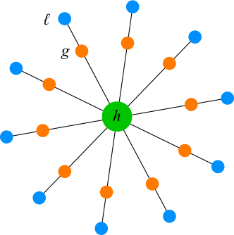
Figure SI.1: An extended star graph with $n=10$

$$\begin{cases}\tau_{hg}=1+\frac{1}{2n}\Big{[}(n-1)\tau_{gg^{\prime}}\Big{]}+\frac{1}{4}\Big{[}\tau_{h\ell}\Big{]}\\ \tau_{h\ell}=1+\frac{1}{2n}\Big{[}(n-1)\tau_{g\ell^{\prime}}+\tau_{g\ell}\Big{]}+\frac{1}{2}\Big{[}\tau_{hg}\Big{]}\\ \tau_{\ell\ell^{\prime}}=1+\frac{2}{2}\Big{[}\tau_{g\ell^{\prime}}\Big{]}\\ \tau_{gg^{\prime}}=1+\frac{2}{4}\Big{[}\tau_{g\ell^{\prime}}+\tau_{hg}\Big{]}\\ \tau_{g\ell}=1+\frac{1}{4}\Big{[}\tau_{h\ell}\Big{]}\\ \tau_{g\ell^{\prime}}=1+\frac{1}{4}\Big{[}\tau_{h\ell}+\tau_{\ell\ell^{\prime}}\Big{]}+\frac{1}{2}\Big{[}\tau_{gg^{\prime}}\Big{]}.\end{cases}$$ (11)

Solving this system and plugging the results into (7), we get

$$\begin{cases}\tau_{h}=\,\displaystyle\frac{64n(3n-1)}{12n^{2}+35n+1}\\ \\ \tau_{g}=\,\displaystyle\frac{8n(17n-1)}{12n^{2}+35n+1}\\ \\ \tau_{\ell}=\,\displaystyle\frac{16n(3+5n)}{12n^{2}+35n+1}\end{cases}$$ (12)

It is also straightforward to see that $p_{h}=p_{\ell}=\frac{1}{2}$, and ${p_{g}=\frac{n+1}{2n}}$. Inserting these values into Equation (8), we get:

$$b^{*}=\,\displaystyle\frac{56n^{2}-39n-1}{22n^{2}-20n-2}$$ (13)

Which means that in the large $n$ limit, $b^{*}$ approaches $28/11$.

S2.C Imperfect extended star graph

We consider the previous setup, but instead of attaching a new node to every node that is adjacent to hub, we only do so for $n_{g}$ of them. So, the graph comprises a hub, $n_{g}$ nodes with degree 2 that are connected to a hub and to a leaf node, and ${n-n_{g}}$ nodes with degree 1 that are connected directly to the hub. An example graph with $n=10$ and $n_{g}=3$ is depicted in Figure SI.2. We denote the leafs connected to degree-2 nodes with $d$ and we denote the leafs directly connected to the hub by $p$. The quantities of interest are $\tau_{pp^{\prime}}$ (between two $p$ nodes), $\tau_{ph}$, $\tau_{pg}$, $\tau_{pd}$, $\tau_{hg}$, $\tau_{hd}$, $\tau_{gg^{\prime}}$ (between two $g$ nodes), $\tau_{gd}$ (between a $g$ node and its adjacent $d$-node), $\tau_{gd^{\prime}}$ (between a $g$ node and a $d$-node adjacent to another $g$ node), $\tau_{dd^{\prime}}$ (between two $d$ nodes attached to the same $g$-node), and $\tau_{dd^{\prime\prime}}$ (between two $d$-nodes adjacent to two distinct $g$ nodes). The system of equations to solve for the remeeting times is the following:

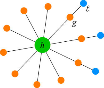
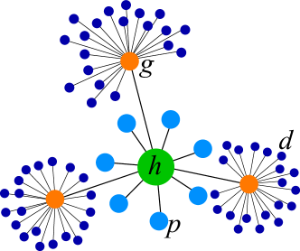
Figure SI.2: An example imperfect extended star graph with $n=10$ and $n_{g}=3$

$$\begin{cases}\tau_{pp^{\prime}}=1+\frac{2}{2}\tau_{ph}\\ \tau_{ph}+1+\frac{1}{2n}\Big{[}(n-n_{g}-1)\tau_{pp^{\prime}}+n_{g}\tau_{pg}\Big{]}\\ \tau_{pg}=1+\frac{1}{2}\Big{[}\tau_{hg}+\frac{1}{4}\Bigg{[}\tau_{pd}+\tau_{ph}\Big{]}\\ \tau_{pd}=1+\frac{1}{2}\tau_{hd}+\frac{1}{2}\tau_{pg}\\ \tau_{hg}=1+\frac{1}{2n}\Big{[}(n_{g}-1)\tau_{gg^{\prime}}+(n-n_{g})\tau_{pg}\Big{]}+\frac{1}{4}\tau_{hd}\\ \tau_{hd}=1+\frac{1}{2n}\Big{[}(n_{g}-1)\tau_{gd^{\prime}}+\tau_{gd}+(n-n_{g})\tau_{pd}\Big{]}+\frac{1}{2}\tau_{hg}\\ \tau_{gg^{\prime}}=1+\frac{1}{2}\Big{[}\tau_{hg}+\tau_{gd^{\prime}}\Big{]}\tau_{gd^{\prime}}=1+\frac{1}{4}\Big{[}\tau_{hd}+\tau_{dd^{\prime}}\Big{]}+\frac{1}{2}\tau_{gg^{\prime}}\\ \tau_{gd}=1+\frac{1}{4}\tau_{hd}\\ \tau_{dd^{\prime}}=1+\tau_{gd^{\prime}}.\end{cases}$$ (14)

(15)

Using these values, we arrive at

(16)

A more compact way to represent the result is with two matrices for the polynomial coefficients of the numerator and the denominator. For the numerator, the $i-j$ element of the following matrix yields the coefficient of $n^{i-1}n_{g}^{j-1}$ in the numerator:

$$\left[\begin{array}[]{ccccc}0&0&0&0&0\\ 0&-7&-20&9&2\\ -7&-325&108&56&0\\ -225&-365&438&0&0\\ 96&712&0&0&0\\ 136&0&0&0&0\\ \end{array}\right]$$ (23)

and for the denominator we have:

$$\left[\begin{array}[]{ccccc}0&0&0&11&-3\\ 0&-28&106&-41&-1\\ 0&-445&141&-12&0\\ 0&-269&185&0&0\\ 0&356&0&0&0\\ \end{array}\right]$$ (29)

For $n_{g}\ll n$, we have:

$$b^{*}=\frac{34}{89n_{g}}n+\frac{28539n_{g}+8845}{15842n_{g}}+O\left(\,\displaystyle\frac{1}{n}\right)\approx\,\displaystyle\frac{0.38}{n_{g}}n+\left(1.80+\frac{0.56}{n_{g}}\right)+O\left(\,\displaystyle\frac{1}{n}\right).$$ (30)

For example, if there is only one gate node, that is, $n_{g}=1$, we have

$$b^{*}\bigg{|}_{n_{g}=1}=\,\displaystyle\frac{34}{89}n+\,\displaystyle\frac{18692}{7921}+O\left(\,\displaystyle\frac{1}{n}\right)\approx 0.38n+2.36++O\left(\,\displaystyle\frac{1}{n}\right).$$ (31)

S2.D Imperfect star of stars

Consider the previous setup, but instead of attaching one $d$-node to each $g$-node, we attach $n_{d}$ of them to each $g$-node. So, the number of $g$-nodes is still $n_{g}$, but the number of $d$-nodes is now ${n_{g}\times n_{d}}$.

An example graph with $n=10$, $n_{g}=3$ , and $n_{d}=20$ is depicted in Figure SI.3. The quantities of interest are $\tau_{pp^{\prime}}$ (between two $p$ nodes), $\tau_{ph}$, $\tau_{pg}$, $\tau_{pd}$, $\tau_{hg}$, $\tau_{hd}$, $\tau_{gg^{\prime}}$ (between two $g$ nodes), $\tau_{gd}$ (between a $g$ node and its adjacent $d$-node), $\tau_{gd^{\prime}}$ (between a $g$ node and a $d$-node adjacent to another $g$ node), $\tau_{dd^{\prime}}$ (between two $d$ nodes attached to the same $g$-node), and $\tau_{dd^{\prime\prime}}$ (between two $d$-nodes adjacent to two distinct $g$ nodes). The system of equations to solve for the remeeting times is the following:

Figure SI.3: An example of imperfect star of stars, with $n=10$, $n_{g}=3$ , and $n_{d}=20$

$$\begin{cases}\tau_{pp^{\prime}}=1+\frac{2}{2}\tau_{ph}\\ \tau_{ph}+1+\frac{1}{2n}\Big{[}(n-n_{g}-1)\tau_{pp^{\prime}}+n_{g}\tau_{pg}\Big{]}\\ \tau_{pg}=1+\frac{1}{2}\Big{[}\tau_{hg}+\frac{1}{2(n_{d}+1)}\Bigg{[}n_{d}\tau_{pd}+\tau_{ph}\Big{]}\\ \tau_{pd}=1+\frac{1}{2}\tau_{hd}+\frac{1}{2}\tau_{pg}\\ \tau_{hg}=1+\frac{1}{2n}\Big{[}(n_{g}-1)\tau_{gg^{\prime}}+(n-n_{g})\tau_{pg}\Big{]}+\frac{1}{2(n_{d}+1)}n_{d}\tau_{hd}\\ \tau_{hd}=1+\frac{1}{2n}\Big{[}(n_{g}-1)\tau_{gd^{\prime}}+\tau_{gd}+(n-n_{g})\tau_{pd}\Big{]}+\frac{1}{2}\tau_{hg}\\ \tau_{gg^{\prime}}=1+\frac{1}{n_{d}+1}\Big{[}\tau_{hg}+n_{d}\tau_{gd^{\prime}}\Big{]}\tau_{gd^{\prime}}=1+\frac{1}{2(n_{d}+1)}\Big{[}\tau_{hd}+n_{d}\tau_{dd^{\prime\prime}}\Big{]}+\frac{1}{2}\tau_{gg^{\prime}}\\ \tau_{gd}=1+\frac{1}{2(n_{d}+1)}\Big{[}\tau_{hd}+(n_{d}-1)\tau_{dd^{\prime}}\Big{]}\\ \tau_{dd^{\prime}}=1+\tau_{gd}\\ \tau_{dd^{\prime\prime}}=1+\tau_{gd^{\prime}}\end{cases}$$ (32)

The expressions for the solution to this system are long, so we only present the final solution after inserting into Equation (8). We have:

$$b^{*}=\frac{\alpha}{\beta},$$ (33)

where the numerator is given by:

$$\alpha=n^{5}\bigg{[}16n_{d}^{3}+82n_{d}^{2}+120n_{d}+54\bigg{]}$$

$$+n^{4}\bigg{[}n_{g}(112n_{d}^{4}+460n_{d}^{3}+600n_{d}^{2}+252n_{d})+16n_{d}^{4}+74n_{d}^{3}+92n_{d}^{2}+22n_{d}-12\bigg{]}$$

$$+\leavevmode\resizebox{411.93767pt}{}{$n^{3}\bigg{[}n_{g}^{2}(48n_{d}^{5}+256n_{d}^{4}+390n_{d}^{3}+182n_{d}^{2})+n_{g}(-32n_{d}^{5}-138n_{d}^{4}-256n_{d}^{3}-227n_{d}^{2}-77n_{d})+-16n_{d}^{4}-90n_{d}^{3}-171n_{d}^{2}-135n_{d}-38\bigg{]}$}$$

$$+\leavevmode\resizebox{411.93767pt}{}{$n^{2}\bigg{[}n_{g}^{3}(22n_{d}^{5}+56n_{d}^{4}+34n_{d}^{3})+n_{g}^{2}(28n_{d}^{5}+80n_{d}^{4}+80n_{d}^{3}+28n_{d}^{2})+n_{g}(-16n_{d}^{5}-108n_{d}^{4}-238n_{d}^{3}-217n_{d}^{2}-71n_{d})-3n_{d}^{2}-7n_{d}-4\bigg{]}$}$$

$$+\leavevmode\resizebox{411.93767pt}{}{$n\bigg{[}n_{g}^{4}(2n_{d}^{5}+2n_{d}^{4})+n_{g}^{3}(4n_{d}^{5}+9n_{d}^{4}+5n_{d}^{3})+n_{g}^{2}(-2n_{d}^{5}-11n_{d}^{4}-18n_{d}^{3}-9n_{d}^{2})+n_{g}(-3n_{d}^{3}-7n_{d}^{2}-4n_{d})\bigg{]}$}.$$ (34)

$$\beta=n^{4}\Big{[}n_{g}\left(64n_{d}^{4}+256n_{d}^{3}+296n_{d}^{2}+96n_{d}\right)\Big{]}$$

$$+n^{3}\Big{[}n_{g}^{2}\left(32n_{d}^{5}+148n_{d}^{4}+162n_{d}^{3}+28n_{d}^{2}\right)+n_{g}\left(-32n_{d}^{5}-148n_{d}^{4}-226n_{d}^{3}-124n_{d}^{2}-8n_{d}\right)\Big{]}$$

$$+\leavevmode\resizebox{411.93767pt}{}{$n^{2}\Big{[}n_{g}^{3}\left(4n_{d}^{5}-6n_{d}^{4}-22n_{d}^{3}\right)+n_{g}^{2}\left(28n_{d}^{5}+98n_{d}^{4}+108n_{d}^{3}+48n_{d}^{2}\right)+n_{g}\left(-32n_{d}^{5}-180n_{d}^{4}-342n_{d}^{3}-264n_{d}^{2}-72n_{d}\right)\Big{]}$}$$

$$+n_{g}^{4}\left(-2n_{d}^{5}-4n_{d}^{4}\right)+n_{g}^{3}\left(2n_{d}^{5}+12n_{d}^{4}+8n_{d}^{3}\right)$$ (35)

Suppose there are many leafs but very few gates: $n_{g}\ll n_{d}=\mu n$, where $\mu$ is of $O(1)$. That is, $n$ and $n_{d}$ are of the same order of magnitude and are both much greater than $n_{g}$. We can use the following expansion:

$$b^{*}=\frac{\mu+\mu^{2}n_{g}(3n_{g}-2)+7\mu n_{g}+1}{2\mu n_{g}(\mu(n_{g}-1)+2)}+O\left(\frac{n_{g}}{n}\right)$$ (36)

Maintaining the previous regime, we can expand this in $n_{g}$ as follows:

$$b^{*}=\frac{3}{2}+\left(\frac{1}{2}+\frac{1}{2\mu}\right)\frac{1}{n_{g}}+O\left(\frac{1}{n_{g}^{2}}\right)+O\left(\frac{n_{g}}{n}\right).$$ (37)

Since the average degree approaches 2 in the regime considered above, the graph is a significant promoter of cooperation because $b^{*}$ (which approaches $3/2$) is smaller than the average degree.

In the regime $n_{g}\ll n\ll n_{d}$, too, we find that $b^{*}$ is smaller than average degree. In this regime, we have:

$$b^{*}=\frac{3}{2}+\frac{1}{2(n_{g}-1)}+O\left(\frac{n_{g}}{n}\right)+O\left(\frac{n}{n_{d}}\right)$$ (38)

S2.E Star of stars

If we take the solution of the last section and set $n_{g}$ and $n$ equal, the resulting graph is a star of stars, that is, a hub that is connected to $n$ nodes, and each of these $n$ nodes is a hub to a star of $n_{d}$ nodes. The critical benefit to cost ratio simplifies to the following:

$$b^{*}=\,\displaystyle\frac{n^{2}\Big{(}12n_{d}^{3}+47n_{d}^{2}+44n_{d}+9\Big{)}-n\Big{(}6n_{d}^{3}+31n_{d}^{2}+33n_{d}+8\Big{)}-\big{(}n_{d}+1\big{)}}{2n_{d}(n-1)\Big{[}2+n(3n_{d}+8)(n_{d}+1)\Big{]}}$$ (39)

For $n\ll n_{d}$, we can use the following expansion

$$b^{*}=\left(2+\frac{1}{n-1}\right)+\left(\frac{1}{1-n}+\frac{1}{2}\right)\frac{1}{n_{d}}+O\left(\frac{1}{n_{d}^{2}}\right).$$ (40)

So $b^{*}$ approaches ${2+1/(n-1)}$ as $n_{d}$ grows. The average degree, on the other hand, approaches 2 from above as $n_{d}$ grows. So $b^{*}$ never becomes smaller than the average degree.

S2.F Three-layer extended star

Consider the extended star, but with three layers instead of two. There is one hub $h$, attached to $n$ nodes $g$ in the first layer, there are $n$ nodes $G$ in the second layer each connected to one $g$ nodes, and there are $n$ nodes $\ell$ in the third layer each attached to a $G$ node. Figure SI.4 depicts an example case with $n=10$. The remeeting times of interest are: $\tau_{\ell\ell^{\prime}}$ (between two $\ell$ nodes), $\tau_{G\ell}$ (between a $G$ node and its adjacent $\ell$ node), $\tau_{G^{\prime}\ell}$ (between a $G$ node and an $\ell$ node not adjacent to it), $\tau_{g\ell}$ (between a $g$ node and an $\ell$ node on the same spoke), $\tau_{g^{\prime}\ell}$ (between a $g$ node and an $\ell$ node on another spoke), $\tau_{h\ell}$ (between the hub and an $\ell$ node), $\tau_{gG}$ (between a $g$ node and its adjacent $G$ node), $\tau_{gg^{\prime}}$ (between two distinct $g$ nodes), $\tau_{gh}$ (between the hub and a $g$ node), $\tau_{GG^{\prime}}$ (between two distinct $G$ nodes), $\tau_{Gg^{\prime}}$ (between a $G$ node and a $g$ node on another spoke), and $\tau_{Gh}$ (between the hub and a $g$ node).

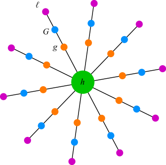
Figure SI.4: An example three-layer extended star graph with $n=10$

$$\begin{cases}\tau_{\ell\ell^{\prime}}=1+\tau_{G^{\prime}\ell}\\ \tau_{G\ell}=1+\frac{1}{4}\tau_{g\ell}\\ \tau_{G^{\prime}\ell}=1+\frac{1}{4}\big{[}\tau_{\ell\ell^{\prime}}+\tau_{g^{\prime}\ell}\big{]}+\frac{1}{2}\tau_{GG^{\prime}}\\ \tau_{g\ell}=1+\frac{1}{4}\big{[}\tau_{h\ell}+\tau_{G\ell}\big{]}+\frac{1}{2}\tau_{gG}\\ \tau_{g^{\prime}\ell}=1+\frac{1}{4}\big{[}\tau_{G^{\prime}\ell}+\tau_{h\ell}\big{]}+\frac{1}{2}\tau_{Gg^{\prime}}\\ \tau_{h\ell}=1+\frac{1}{2n}\big{[}\tau_{g\ell}+(n-1)\tau_{g^{\prime}\ell}\big{]}+\frac{1}{2}\tau_{Gh}\\ \tau_{gG}=1+\frac{1}{4}\big{[}\tau_{Gh}+\tau_{g\ell}\big{]}\\ \tau_{gg^{\prime}}=1+\frac{1}{2}\big{[}\tau_{Gg^{\prime}}+\tau_{gh}\big{]}\\ \tau_{gh}=1+\frac{1}{2n}\big{[}(n-1)\tau_{gg^{\prime}}\big{]}+\frac{1}{4}\tau_{Gh}\\ \tau_{GG^{\prime}}=1+\frac{1}{2}\big{[}\tau_{G^{\prime}\ell}+\tau_{Gg^{\prime}}\big{]}\\ \tau_{Gg^{\prime}}=1+\frac{1}{4}\big{[}\tau_{g^{\prime}\ell}+\tau_{gg^{\prime}}+\tau_{GG^{\prime}}+\tau_{gG}\big{]}\\ \tau_{Gh}=1+\frac{1}{2n}\big{[}\tau_{gG}+(n-1)\tau_{Gg^{\prime}}\big{]}+\frac{1}{4}\big{[}\tau_{\ell h}+\tau_{gh}\big{]}\end{cases}$$ (41)

The solution leads us to the following result for the critical benefit-to-cost ratio:

$$b^{*}=\frac{106940n^{3}-52194n^{2}-4820n+6}{41723n^{3}-18453n^{2}-10790n}$$ (42)

For large $n$, we can use the following expansion:

$$b^{*}=\frac{106940}{41723}-\frac{204326442}{1740808729n}+O\left(\frac{1}{n^{2}}\right)\approx 2.56-\frac{0.12}{n}+O\left(\frac{1}{n^{2}}\right)$$ (43)

S2.G Two stars: hub-to-hub connection

If we have two star graphs, one with $n_{1}$ leafs and the other with $n_{2}$ leafs, we can connect these two graphs in several different ways to restore the faith of cooperation (which is not favored by natural selection in either of the star graphs alone, as shown in Section S2.A above).

First suppose that the hub of the first star is connected to the hub of the other via a link. There are 8 distinct remeeting times to consider: $\tau_{\ell_{1}\ell_{1}^{\prime}}$(between two distinct leafs of the first star), $\tau_{\ell_{1}h_{1}}$ (between a leaf and the hub of the first star), $\tau_{\ell_{1}h_{2}}$ (between a leaf of the first star and the hub of the second star), $\tau_{\ell_{1}\ell_{2}}$ (between a leaf in one star and a leaf in the other), $\tau_{h_{1}h_{2}}$ (between the hubs), $\tau_{h_{1}\ell_{2}}$ (between the hub of the first star and a leaf in the second star), $\tau_{h_{2}\ell_{2}}$ (between a leaf of the second star and its hub), and $\tau_{\ell_{2}\ell_{2}^{\prime}}$ (between two leafs of the second star). The remeeting times satisfy the following system of equations:

$$\begin{cases}\tau_{\ell_{1}\ell_{1}^{\prime}}&=1+\tau_{\ell_{1}h_{1}}\\ \tau_{\ell_{1}h_{1}}&=1+\frac{1}{2(n_{1}+1)}\bigg{[}\tau_{\ell_{1}h_{2}}+(n_{1}-1)\tau_{\ell_{1}\ell 1^{\prime}}\bigg{]}\\ \tau_{\ell_{1}h_{2}}&=1+\frac{1}{2}\tau_{h_{1}h_{2}}+\,\displaystyle\frac{1}{2(n_{2}+1)}\bigg{[}n_{2}\tau_{\ell_{1}\ell_{2}}+\tau_{\ell_{1}h_{1}}\bigg{]}\\ \tau_{\ell_{1}\ell_{2}}&=1+\frac{1}{2}\tau_{h_{1}\ell_{2}}+\frac{1}{2}\tau_{\ell_{1}h_{2}}\\ \tau_{h_{1}h_{2}}&=1+\,\displaystyle\frac{1}{2(n_{1}+1)}\big{[}n_{1}\tau_{\ell_{1}h_{2}}\big{]}+\,\displaystyle\frac{1}{2(n_{2}+1)}\big{[}n_{2}\tau_{h_{1}\ell_{2}}\big{]}\\ \tau_{h_{1}\ell_{2}}&=1+\,\displaystyle\frac{1}{2(n_{1}+1)}\bigg{[}n_{1}\tau_{\ell_{1}\ell_{2}}+\tau_{h_{2}\ell_{2}}\bigg{]}+\frac{1}{2}\tau_{h_{1}h_{2}}\\ \tau_{h_{2}\ell_{2}}&=1+\frac{1}{2(n_{2}+1)}\bigg{[}\tau_{h_{1}\ell_{2}}+(n_{2}-1)\tau_{\ell_{2}\ell_{2}^{\prime}}\bigg{]}\\ \tau_{\ell_{2}\ell_{2}^{\prime}}&=1+\tau_{h_{2}\ell_{2}}.\end{cases}$$ (44)

Solving this and inserting into Equation (7) and then plugging the results into Equation (8), we arrive at the solution:

$$b^{*}=\frac{\alpha}{\beta},$$ (45)

where the numerator is

$$\alpha =n_{1}^{5}\Big{(}8n_{2}^{3}+41n_{2}^{2}+60n_{2}+27\Big{)}$$

$$+n_{1}^{4}\Big{(}64n_{2}^{4}+307n_{2}^{3}+551n_{2}^{2}+437n_{2}+129\Big{)}$$

$$+n_{1}^{3}\Big{(}8n_{2}^{5}+307n_{2}^{4}+1170n_{2}^{3}+1686n_{2}^{2}+1042n_{2}+227\Big{)}$$

$$+n_{1}^{2}\Big{(}41n_{2}^{5}+551n_{2}^{4}+1686n_{2}^{3}+2066n_{2}^{2}+1065n_{2}+175\Big{)}$$

$$+n_{1}\Big{(}60n_{2}^{5}+437n_{2}^{4}+1042n_{2}^{3}+1065n_{2}^{2}+450n_{2}+50\Big{)}$$

$$+\Big{(}27n_{2}^{5}+129n_{2}^{4}+227n_{2}^{3}+175n_{2}^{2}+50n_{2}\Big{)},$$ (46)

and the denominator is

$$\beta =n_{1}^{4}\left(32n_{2}^{4}+128n_{2}^{3}+148n_{2}^{2}+48n_{2}\right)$$

$$+n_{1}^{3}\left(128n_{2}^{4}+480n_{2}^{3}+544n_{2}^{2}+188n_{2}\right)$$

$$+n_{1}^{2}\left(148n_{2}^{4}+544n_{2}^{3}+636n_{2}^{2}+240n_{2}\right)$$

$$+n_{1}\left(48n_{2}^{4}+188n_{2}^{3}+240n_{2}^{2}+100n_{2}\right).$$ (47)

If the two stars are identical, with $n_{1}=n_{2}=n$, then the expression simplifies to:

$$b^{*}=\,\displaystyle\frac{(n+1)^{2}(10n^{2}+17n+5)}{4n^{4}+12n^{3}+11n^{2}+5n}.$$ (48)

When $n$ is large, this converges to $10/4$. With first-order correction in the large-$n$ limit, we can write

$$b^{*}=\frac{5}{2}+\frac{7}{4n}+O\left(\frac{1}{n^{2}}\right).$$ (49)

If the stars are not identical, but both are very large, such that $n_{1}=n$ and $n_{2}=\alpha n$, the in the limit as ${n\rightarrow\infty}$, we have:

$$b^{*}=\left(2+\,\displaystyle\frac{1}{4\alpha}+\,\displaystyle\frac{\alpha}{4}\right)+\,\displaystyle\frac{(\alpha+1)(9\alpha^{2}+10\alpha+9)}{32\alpha^{2}n}+O\left(\frac{1}{n^{2}}\right)$$ (50)

S2.H Two stars: hub-to-leaf connection

I In the previous scenario, if instead of connecting the hubs, we connect the hub of the first star to a leaf in the second star, the equations for the remeeting times change. We denote the leaf that is connected to the hub of the first star by $g$. There are 12 distinct remeeting times to consider: $\tau_{\ell_{1}\ell_{1}^{\prime}}$, $\tau_{\ell_{1}h_{1}}$ , $\tau_{\ell_{1}h_{2}}$, $\tau_{\ell_{1}\ell_{2}}$, $\tau_{h_{1}h_{2}}$, $\tau_{h_{1}\ell_{2}}$, $\tau_{h_{2}\ell_{2}}$, $\tau_{\ell_{2}\ell_{2}^{\prime}}$, $\tau_{\ell_{1}g}$, $\tau_{h_{1}g}$, $\tau_{gh_{2}}$, and $\tau_{g\ell_{2}}$. Without loss or generality, we consider the case where the second star has size $n_{2}+1$. Equivalently, we can assume the stars have sizes $n_{1}$ and $n_{2}$, and the hubs are being connected via one intermediary node. This is merely for aesthetic reasons: with this change of notation, the analysis will be manifest-symmetric in $n_{1}$ and $n_{2}$. The remeeting times satisfy the following system of equations:

$$\begin{cases}\tau_{\ell_{1}\ell_{1}^{\prime}}&=1+\tau_{\ell_{1}h_{1}}\\ \tau_{\ell_{1}h_{1}}&=1+\frac{1}{2(n_{1}+1)}\bigg{[}\tau_{\ell_{1}g}+(n_{1}-1)\tau_{\ell_{1}\ell 1^{\prime}}\bigg{]}\\ \tau_{\ell_{1}h_{2}}&=1+\frac{1}{2}\tau_{h_{1}h_{2}}+\,\displaystyle\frac{1}{2(n_{2}+1)}\bigg{[}n_{2}\tau_{\ell_{1}\ell_{2}}+\tau_{\ell_{1}g}\bigg{]}\\ \tau_{\ell_{1}\ell_{2}}&=1+\frac{1}{2}\tau_{h_{1}\ell_{2}}+\frac{1}{2}\tau_{\ell_{1}h_{2}}\\ \tau_{h_{1}h_{2}}&=1+\,\displaystyle\frac{1}{2(n_{1}+1)}\big{[}n_{1}\tau_{\ell_{1}h_{2}}+\tau_{gh_{2}}\big{]}+\,\displaystyle\frac{1}{2(n_{2}+1)}\big{[}n_{2}\tau_{h_{1}\ell_{2}}+\tau_{h_{1}g}\big{]}\\ \tau_{h_{1}\ell_{2}}&=1+\,\displaystyle\frac{1}{2(n_{1}+1)}\bigg{[}n_{1}\tau_{\ell_{1}\ell_{2}}+\tau_{g\ell_{2}}\bigg{]}+\frac{1}{2}\tau_{h_{1}h_{2}}\\ \tau_{h_{2}\ell_{2}}&=1+\frac{1}{2(n_{2}+1)}\bigg{[}\tau_{g\ell_{2}}+(n_{2}-1)\tau_{\ell_{2}\ell_{2}^{\prime}}\bigg{]}\\ \tau_{\ell_{2}\ell_{2}^{\prime}}&=1+\tau_{h_{2}\ell_{2}}\\ \tau_{\ell_{1}g}&=1+\frac{1}{2}\tau_{h_{1}g}+\frac{1}{4}\bigg{[}\tau_{\ell_{1}h_{1}}+\tau_{\ell_{1}h_{2}}\bigg{]}\\ \tau_{h_{1}g}&=1+\,\displaystyle\frac{1}{2(n_{1}+1)}n_{1}\tau_{\ell_{1}g}+\frac{1}{4}\tau_{h_{1}h_{2}}\\ \tau_{gh_{2}}&=1+\frac{1}{2(n_{2}+1)}n_{2}\tau_{g\ell_{2}}+\frac{1}{4}\tau_{h_{1}h_{2}}\\ \tau_{g\ell_{2}}&=1+\frac{1}{2}\tau_{gh_{2}}+\frac{1}{4}\bigg{[}\tau_{h_{1}\ell_{2}}+\tau_{h_{2}\ell_{2}}\bigg{]}.\end{cases}$$ (51)

Solving this and using Equation (8), we arrive at

$$b^{*}=\frac{\alpha}{\beta},$$ (52)

where the numerator is

$$\alpha =n_{1}^{6}\Big{(}288n_{2}^{4}+1746n_{2}^{3}+3738n_{2}^{2}+3402n_{2}+1122\Big{)}$$

$$n_{1}^{5}\Big{(}2880n_{2}^{5}+19566n_{2}^{4}+53836n_{2}^{3}+74006n_{2}^{2}+50424n_{2}+13568\Big{)}$$

$$+n_{1}^{4}\Big{(}288n_{2}^{6}+19566n_{2}^{5}+113908n_{2}^{4}+276152n_{2}^{3}+338086n_{2}^{2}+207330n_{2}+50766\Big{)}$$

$$+n_{1}^{3}\Big{(}1746n_{2}^{6}+53836n_{2}^{5}+276152n_{2}^{4}+610544n_{2}^{3}+687478n_{2}^{2}+389244n_{2}+88248\Big{)}$$

$$+n_{1}^{2}\Big{(}3738n_{2}^{6}+74006n_{2}^{5}+338086n_{2}^{4}+687478n_{2}^{3}+716764n_{2}^{2}+375760n_{2}+78656\Big{)}$$

$$+n_{1}\Big{(}3402n_{2}^{6}+50424n_{2}^{5}+207330n_{2}^{4}+389244n_{2}^{3}+375760n_{2}^{2}+181328n_{2}+34504\Big{)}$$

$$+\Big{(}1122n_{2}^{6}+13568n_{2}^{5}+50766n_{2}^{4}+88248n_{2}^{3}+78656n_{2}^{2}+34504n_{2}+577\Big{)},$$ (53)

and the denominator is

$$\beta =n_{1}^{5}\left(1152n_{2}^{5}+7200n_{2}^{4}+17472n_{2}^{3}+20778n_{2}^{2}+12285n_{2}+2937\right)$$

$$n_{1}^{4}\left(7200n_{2}^{5}+43072n_{2}^{4}+99734n_{2}^{3}+112892n_{2}^{2}+63433n_{2}+14437\right)$$

$$+n_{1}^{3}\left(17472n_{2}^{5}+99734n_{2}^{4}+218830n_{2}^{3}+232766n_{2}^{2}+121788n_{2}+25666\right)$$

$$+n_{1}^{2}\left(20778n_{2}^{5}+112892n_{2}^{4}+232766n_{2}^{3}+228350n_{2}^{2}+107262n_{2}+19648\right)$$

$$+n_{1}\left(12285n_{2}^{5}+63433n_{2}^{4}+121788n_{2}^{3}+107262n_{2}^{2}+42048n_{2}+5472\right)$$

$$+2937n_{2}^{5}+14437n_{2}^{4}+25666n_{2}^{3}+19648n_{2}^{2}+5472n_{2}.$$ (54)

If the stars are identical, that is, if we have two stars each with $n$ leafs and then we connect their hubs through a gate node, then we have

$$b^{*}=\,\displaystyle\frac{(n+1)(36n^{2}+90n+19)}{4n(3n^{2}+11n+9)}=3-\,\displaystyle\frac{1}{2n}+O\left(\frac{1}{n^{2}}\right)$$ (55)

So as the size of the stars goes to infinity, the value of $b^{*}$ approaches 3.

If the stars are not identical but both are large, with $n_{1}=n$ and $n_{2}=\lambda n$, then we have

$$b^{*}=\left(\,\displaystyle\frac{5}{2}+\,\displaystyle\frac{1}{4\lambda}+\,\displaystyle\frac{\lambda}{4}\right)+\,\displaystyle\frac{(\lambda+1)(\lambda+3)(3\lambda+1)}{64\lambda^{2}n}+O\left(\frac{1}{n^{2}}\right).$$ (56)

S2.I Ring of stars: a super-promoter of cooperation

Suppose there are $L$ stars, each with $n$ leafs. We situate these on a ring by connecting the hubs. An example with $n=10$ and $L=5$ is illustrated in Figure SI.5. We define the following remeeting times:

• $\tau_{hh}(x)$ is between the hubs of two stars which are $x$ apart on the ring. For example, two adjacent hubs have remeeting times $\tau_{hh}(1)$.

• $\tau_{h\ell}(x)$ is between a hub and a leaf of a star that is $x$ apart. For example, for the hub and leaf of the same star, we have $\tau_{h\ell}(0)$, and for the leaf of a star and the hub of the neighboring star, we have $\tau_{h\ell}(1)$, and so on.

• $\tau_{\ell\ell}(x)$ is between two distinct leafs, belonging to two stars $x$ apart. So $\tau_{\ell\ell}(0)$ is between two leafs of the same star, $\tau_{\ell\ell}(1)$ is between a leaf in one star and a leaf in a neighboring star.

Note that $x$ varies between 0 and $L$.

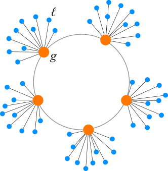
Figure SI.5: An example case of ring of stars with $n=10$ and $L=5$

The recurrence relations that we need to solve have the form of three-dimensional difference equation:

$$\begin{cases}\text{for }x=2\ldots L-2:~{}&\begin{cases}\tau_{hh}(x)=1+\frac{1}{n+2}\bigg{[}\tau_{hh}(x-1)+\tau_{hh}(x+1)+n\tau_{h\ell}(x)\bigg{]}\\ \\ \tau_{h\ell}(x)=1+\,\displaystyle\frac{1}{2(n+2)}\bigg{[}n\tau_{\ell\ell}(x)+\tau_{h\ell}(x+1)+\tau_{h\ell}(x-1)\bigg{]}+\frac{1}{2}\tau_{hh}(x)\\ \\ \tau_{\ell\ell}(x)=1+\tau_{h\ell(x)}\end{cases}\\ \\ \text{for }x<2:~{}&\begin{cases}\tau_{hh}(1)=1+\frac{1}{n+2}\bigg{[}\tau_{hh}(2)+n\tau_{h\ell}(1)\bigg{]}\\ \\ \tau_{h\ell}(1)=1+\,\displaystyle\frac{1}{2(n+2)}\bigg{[}n\tau_{\ell\ell}(1)+\tau_{h\ell}(2)+\tau_{h\ell}(0)\bigg{]}+\frac{1}{2}\tau_{hh}(1)\\ \\ \tau_{h\ell}(0)=1+\,\displaystyle\frac{1}{2(n+2)}\bigg{[}(n-1)\tau_{\ell\ell}(0)+2\tau_{h\ell}(1)\bigg{]}\\ \\ \tau_{\ell\ell}(0)=1+\tau_{h\ell}(0)\end{cases}\end{cases}.$$ (57)

This is a system of linear difference equations with constant coefficients. So the standard way is inserting the ansatz in the form of $r^{x}$ and solving the resulting characteristic equation for $r$. If there is no degenerate root, the solution will take the form ${\sum_{i}a_{i}r_{i}^{x}}$, and we will have to add this to a particular solution for the nonhomogenous system. We use the following ansatz:

$$\begin{cases}\tau_{hh}(x)=\xi_{hh}r^{x}\\ \tau_{h\ell}(x)=\xi_{h\ell}r^{x}\\ \tau_{\ell\ell}(x)=\xi_{\ell\ell}r^{x}\end{cases}~{}~{}1<x<L$$ (58)

This leads to the following characteristic equation:

$$(r-1)^{2}\bigg{[}r^{2}-2(n+2)r+1\bigg{]}=0\Longrightarrow\begin{cases}r_{1}=0\\ r_{2}=0\\ r_{3}=n+2+\sqrt{(n+1)(n+3)}\\ r_{4}=\,\displaystyle\frac{1}{r_{3}}\end{cases}.$$ (59)

This has root zero with degeneracy two. This means that the particular solution to the nonhomogenous equation will be quadratic in $x$. For brevity of notation, let us define:

$$\begin{cases}\lambda\stackrel{{\scriptstyle\text{def}}}{{=}}\sqrt{(n+1)(n+3)},\\ R\stackrel{{\scriptstyle\text{def}}}{{=}}n+2+\sqrt{(n+1)(n+3)}.\end{cases}$$ (60)

Thus we plug in the following form for the solutions:

$$\begin{cases}\tau_{hh}(x)=A_{hh}x^{2}+B_{hh}x+C_{hh}+D_{hh}\big{(}R^{x}+R^{L-x}\big{)}\\ \tau_{h\ell}(x)=A_{h\ell}x^{2}+B_{h\ell}x+C_{h\ell}+D_{h\ell}\big{(}R^{x}+R^{L-x}\big{)}\\ \tau_{\ell\ell}(x)=A_{h\ell}x^{2}+B_{h\ell}x+C_{h\ell}+D_{h\ell}\big{(}R^{x}+R^{L-x}\big{)}\end{cases}$$ (61)

Plugging these into Equations (135), and setting the coefficients of different powers of $x$ and also those of $R^{x}$ and $R^{-x}$ identical to zero (because the equations hold for every $x$ and the functions are linearly independent), and also using the requirement that $\tau_{hh}(x)$ must be equal to ${\tau_{hh}(L-x)}$ (and same for $\tau_{h\ell}$ and $\tau_{\ell\ell}$), we obtain:

$$A_{hh}=A_{\ell\ell}=A_{h\ell}=-(n+1),$$

$$B_{hh}=B_{\ell\ell}=B_{h\ell}=(n+1)L,$$

$$C_{hh}=\,\displaystyle\frac{n(Ln+L-1)\left(R^{L}+1\right)}{(n+1)R^{L}+n\lambda R^{L}+2\lambda R^{L}+n-n\lambda-2\lambda+1},$$

$$D_{hh}=-\frac{n(Ln+L-1)}{(n+1)R^{L}+n\lambda R^{L}+2\lambda R^{L}+n-n\lambda-2\lambda+1}$$

$$D_{h\ell}=\frac{(n+2)(Ln+L-1)}{(n+1)R^{L}+n\lambda R^{L}+2\lambda R^{L}+n-n\lambda-2\lambda+1}$$

$$\leavevmode\resizebox{433.62pt}{}{$\tau_{h\ell}(0)=\frac{-18\lambda+(10\lambda+n(17\lambda+2n(5\lambda+n(R+5)+18)+41))R^{L}+17R^{L}+2L(n+1)^{2}(4\lambda+2n(\lambda+n+4)+7)\left(R^{L}+1\right)-n(29\lambda+2n(7(\lambda+4)+n(\lambda+n+9))+71)-31}{-10\lambda+(18\lambda+n(29\lambda+2n(7(\lambda+4)+n(\lambda+n+9))+71))R^{L}+31R^{L}-n(17\lambda+2n(5\lambda+n(\lambda+n+7)+18)+41)-17}$}.$$ (62)

Using these values, we arrive at the

$$b^{*}=\,\displaystyle\frac{\alpha}{\beta},$$ (63)

where the numerator is

$$\alpha=(n+2)^{2}\Bigg{[}L(n+1)\bigg{(}-2(n(2n+11)+13)R^{L}+(n(\lambda+2n+9)+11)R^{2L}+2n^{2}-\lambda n+9n+11\bigg{)}$$

$$+2R^{L}(n^{2}(n+9)+28n+26)-R^{2L}\Big{(}n^{2}(n+9)+n(\lambda+24)+22\Big{)}-n^{3}-9n^{2}+\lambda n-24n-22\Bigg{]},$$ (64)

and the denominator is:

$$\beta=2\Bigg{[}L(n+1)\bigg{(}-2(n^{4}+7n^{3}+19n^{2}+24n+13)(\lambda+n+2)^{L}$$

$$+\big{(}n^{4}+7n^{3}+17n^{2}+(\lambda+20)n+11\big{)}(\lambda+n+2)^{2L}+n^{4}+7n^{3}+17n^{2}-\lambda n+20n+11\bigg{)}$$

$$+2(n+2)(n^{4}+9n^{3}+30n^{2}+44n+26)(\lambda+n+2)^{L}$$

$$-\Big{(}n^{5}+11n^{4}+46n^{3}+94n^{2}+(\lambda+98)n+44\Big{)}(\lambda+n+2)^{2L}$$

$$-n^{5}-11n^{4}-46n^{3}-94n^{2}+\lambda n-98n-44\Bigg{]}.$$ (65)

For large $n$, we can expand the result in powers of $1/n$. We have:

$$b^{*}=\,\displaystyle\frac{3L-1}{2L-2}+\left[\,\displaystyle\frac{2L^{2}+L+3}{2(L-1)^{2}}\right]\,\displaystyle\frac{1}{n}-\left[\,\displaystyle\frac{3L^{3}-6L^{2}-15L-18}{4(L-1)^{3}}\right]\,\displaystyle\frac{1}{n^{2}}+O\left(\,\displaystyle\frac{1}{n^{2}}\right).$$ (66)

So in the limit as ${n\rightarrow\infty}$, the critical benefit-to-cost ratio approaches ${\frac{3L-1}{2L-2}}$. If $L$ is also large, this approaches $\frac{3}{2}$. Note that the average degree is:

$$\overline{k}=\,\displaystyle\frac{L(n+2)+Ln}{L+Ln}=2.$$ (67)

This is particularly interesting because very rarely graphs have critical benefit to cost ratio less than their average degree. A ring of stars does have this property. We call these structure ‘super-promoters of cooperation’.

S3 Cliques

S3.A Single clique (complete graph)

In a complete graph of size $N$, the system of equations (6) reduces to a single equation:

$$\tau_{xy}=1+\,\displaystyle\frac{1}{2(N-1)}(N-2)\tau_{xy}+\,\displaystyle\frac{1}{2(N-1)}(N-2)\tau_{xy}.$$ (68)

This yields $\tau_{xy}=N-1$. Thus from (7) we get ${\tau_{x}=N}$. Plugging this into (8), we get ${N(N-1)(N-2)}$ in the numerator and ${-N(N-2)}$ in the denominator. Thus we arrive at:

$$b^{*}_{ave}=-(N-1)<0.$$ (69)

So regardless of $b$ and $c$, natural selection does not favor cooperation on a clique.

S3.B Two cliques conjoined directly

Suppose we have a clique of size $n_{1}$ and another clique of size $n_{2}$, and we connect one node from the first clique to a node in the second one. We denote these two nodes by $g_{1}$ and $g_{2}$. We denote the non-gate nodes in the first clique by $c_{1}$ and those in the second clique by $c_{2}$. The remeeting times we need to find are $\tau_{c_{1},c_{1}^{\prime}}$ (between two commoners in the first clique) and $\tau_{c_{2},c_{2}^{\prime}}$, $\tau_{g_{1},g_{2}}$ (between the gates), $\tau_{c_{1},g_{1}}$, $\tau_{c_{2},g_{2}}$, $\tau_{c_{1},g_{2}}$, $\tau_{g_{1},c_{2}}$, and $\tau_{c_{1},c_{2}}$. The recurrence relations are given by:

$$\begin{cases}\tau_{c_{1},c_{1}^{\prime}}=1+\,\displaystyle\frac{\tau_{c_{1},c_{1}^{\prime}}(n_{1}-3)+\tau_{c1,g1}}{(n_{1}-1)},\\ \\ \tau_{c1,g1}=1+\,\displaystyle\frac{\tau_{c_{1},c_{1}^{\prime}}(n_{1}-2)+\tau_{c_{1},g_{2}}}{2n_{1}}+\,\displaystyle\frac{\tau_{c1,g1}(n_{1}-2)}{2(n_{1}-1)},\\ \\ \tau_{c_{1},c_{2}}=1+\,\displaystyle\frac{\tau_{c_{1},c_{2}}(n_{2}-2)+\tau_{c_{1},g_{2}}}{2(n_{2}-1)}+\,\displaystyle\frac{\tau_{c_{1},c_{2}}(n_{1}-2)+\tau_{g_{1},c_{2}}}{2(n_{1}-1)},\\ \\ \tau_{c_{1},g_{2}}=1+\,\displaystyle\frac{\tau_{c_{1},c_{2}}(n_{2}-1)+\tau_{c1,g1}}{2n_{2}}+\,\displaystyle\frac{\tau_{c_{1},g_{2}}(n_{1}-2)+\tau_{g_{1},g_{2}}}{2(n_{1}-1)},\\ \\ \tau_{g_{1},c_{2}}=1+\,\displaystyle\frac{\tau_{c_{1},c_{2}}(n_{1}-1)+\tau_{c_{2},g_{2}}}{2n_{1}}+\,\displaystyle\frac{\tau_{g_{1},c_{2}}(n_{2}-2)+\tau_{g_{1},g_{2}}}{2(n_{2}-1)},\\ \\ \tau_{g_{1},g_{2}}=1+\,\displaystyle\frac{\tau_{c_{1},g_{2}}(n_{1}-1)}{2n_{1}}+\frac{\tau_{g_{1},c_{2}}(n_{2}-1)}{2n_{2}},\\ \\ \tau_{c_{2},c_{2}^{\prime}}=1+\,\displaystyle\frac{\tau_{c_{2},c_{2}^{\prime}}(n_{2}-3)+\tau_{c_{2},g_{2}}}{(n_{2}-1)},\\ \\ \tau_{c_{2},g_{2}}=1+\,\displaystyle\frac{\tau_{c_{2},c_{2}^{\prime}}(n_{2}-2)+\tau_{g_{1},c_{2}}}{2n_{2}}+\,\displaystyle\frac{\tau_{c_{2},g_{2}}(n_{2}-2)}{2(n_{2}-1)}\end{cases}$$ (70)

The closed-form of the solution is too long to present. For the case of ${n_{1}=n_{2}=n}$, we have

$$b^{*}=n^{2}-\frac{2n^{3}(n-2)}{n(n+1)\left(n^{3}+2n-1\right)-2}.$$ (71)

This can be expanded as

$$b^{*}=n^{2}-\,\displaystyle\frac{2}{n}+\,\displaystyle\frac{6}{n^{2}}+O\left(\,\displaystyle\frac{1}{n^{3}}\right)$$ (72)

This means that $b^{*}\approx n^{2}$ is a good approximation even for moderate values of $n$.

S3.C Two cliques, conjoined via one broker node

If instead of being connected directly, the gate nodes were connected via one intermediary node, then we would have

$$b^{*}=\,\displaystyle\frac{8n^{9}-10n^{8}+37n^{7}-32n^{6}+34n^{5}-76n^{4}+81n^{3}-26n^{2}}{20n^{7}-42n^{6}+104n^{5}-100n^{4}-100n^{3}+222n^{2}-116n+16}.$$ (74)

This can be expanded for large $n$ as follows

$$b^{*}=\,\displaystyle\frac{2}{5}n^{2}+\,\displaystyle\frac{17}{50}n+\,\displaystyle\frac{121}{250}+O\left(\,\displaystyle\frac{1}{n}\right).$$ (75)

S3.D Two cliques conjoined via two intermediary broker nodes

For two identical cliques connected via a chain of two intermediary broker nodes, we can take similar steps. Let $\tau_{cc}$ be the remeeting times between two commoners of the same clique, $\tau_{cg}$ between a commoner and the gate node of the same clique, $\tau_{cb}$ between a commoner and the broker node which is closer (that is, the broker which is connected to the gate node that belongs to the same clique as the commoner), $\tau_{cb^{\prime}}$ between a commoner and the other broker node, $\tau_{cg^{\prime}}$ between a commoner and the gate node of the other clique, $\tau_{cc^{\prime}}$ between a commoner from one clique and a commoner from the other clique, $\tau_{gb}$ between a gate node and the adjacent broker node, $\tau_{gb^{\prime}}$ between a gate node and the non-adjacent broker node, $\tau_{gg^{\prime}}$ between the two gate nodes, $\tau_{bb^{\prime}}$ between the two broker nodes. We also have $k_{b}=2$, $k_{g}=n$, and $k_{c}=n-1$. We have:

$$\begin{cases}\tau_{bb^{\prime}}=\frac{\tau_{gb^{\prime}}}{k_{b}}+1\\ \tau_{cc}=\frac{(n-3)\tau_{cc}+\tau_{cg}}{k_{c}}+1\\ \tau_{cc^{\prime}}=\frac{(n-2)\tau_{cc^{\prime}}+\tau_{cg^{\prime}}}{k_{c}}+1\\ \tau_{gg^{\prime}}=\frac{(n-1)\tau_{cg^{\prime}}+\tau_{gb^{\prime}}}{k_{g}}+1\\ \tau_{cg}=\frac{(n-2)\tau_{cg}}{2k_{c}}+\frac{(n-2)\tau_{cc}+\tau_{cb}}{2k_{g}}+1\\ \tau_{gb}=\frac{\tau_{gb^{\prime}}}{2k_{b}}+\frac{(n-1)\tau_{cb}}{2k_{g}}+1\\ \tau_{cb}=\frac{\tau_{cb^{\prime}}+\tau_{cg}}{2k_{b}}+\frac{(n-2)\tau_{cb}+\tau_{gb}}{2k_{c}}+1\\ \tau_{cb^{\prime}}=\frac{\tau_{cb}+\tau_{cg^{\prime}}}{2k_{b}}+\frac{(n-2)\tau_{cb^{\prime}}+\tau_{gb^{\prime}}}{2k_{c}}+1\\ \tau_{cg^{\prime}}=\frac{(n-2)\tau_{cg^{\prime}}+\tau_{gg^{\prime}}}{2k_{c}}+\frac{(n-1)\tau_{cc^{\prime}}+\tau_{cb^{\prime}}}{2k_{g}}+1\\ \tau_{gb^{\prime}}=\frac{\tau_{gb}+\tau_{gg^{\prime}}}{2k_{b}}+\frac{(n-1)\tau_{cb^{\prime}}+\tau_{bb^{\prime}}}{2k_{g}}+1.\end{cases}$$ (76)

The solution can be expanded for large $n$ as follows:

$$b^{*}=4n-\frac{224}{5}+\frac{42304}{75n}+O\left(\frac{1}{n^{2}}\right)$$ (77)

S3.E Two cliques with longer chains

When the number of intermediary nodes on the connecting chain is comparable to the number of nodes in the cliques, the analytical solutions to the system of linear equations for remeeting times become unwieldy. But numerical solution is straightforward. Figure SI.6 displays the $b^{*}$ values for chains with 2 to 50 intermediary nodes, for different cliques sizes. For large $L$, the values of $b^{*}$ approach 2, and the convergence rate depends on the cliques size. This limiting value of 2 corresponds to an infinite chain (where the effect of the two cliques is also negligible).

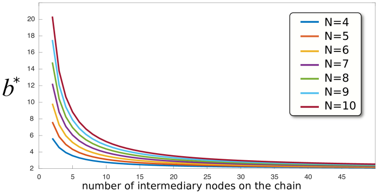
Figure SI.6: Conjoining two cliques with long chains.

S3.F Conjoining large cliques

We showed that conjoining two cliques directly or via one broker nodes leads to a $b^{*}$ that grows with $n$ quadratically. For a single clique, natural selection does not favor cooperation over defection regardless of the benefit-to-cost ratio. Having two intermediary broker nodes does provide a marked reduction in $b^{*}$, lowering the leading behavior of $b^{*}$ to linear in $n$, but we note that for large network sizes, this still might not be feasible. That is, though cooperation is in principle possible, for large cliques, the benefit-to-cot ratio proportional to $n$ might still not be feasible to provide, though it is considerably better than a single clique.

S3.G Star of cliques

Suppose there are $m$ identical cliques each with $m$ nodes, and there is a hub node that is connected to one gate node in each community. So there are $m$ gate nodes overall, one for each community. An example case with $m=5$ and $n=10$ is depicted in Figure SI.7.

$$\begin{cases}\tau_{gh}=1+\frac{(m-1)\tau_{gg^{\prime}}}{2m}+\frac{(n-1)\tau_{hc}}{2n}\\ \tau_{hc}=1+\frac{(m-1)\tau_{gc^{\prime}}+\tau_{gc}}{2m}+\frac{(n-2)\tau_{hc}+\tau_{gh}}{2(n-1)}\\ \tau_{cc}=1+\frac{(n-3)\tau_{cc}+\tau_{gc}}{n-1}\\ \tau_{gc}=1+\frac{(n-2)\tau_{gc}}{2(n-1)}+\frac{(n-2)\tau_{cc}+\tau_{hc}}{2n}\\ \tau_{gg^{\prime}}=1+\frac{(n-1)\tau_{gc^{\prime}}+\tau_{gh}}{n}\\ \tau_{cc^{\prime}}=1+\frac{(n-2)\tau_{cc^{\prime}}+\tau_{gc^{\prime}}}{n-1}\\ \tau_{gc^{\prime}}=1+\frac{(n-2)\tau_{gc^{\prime}}+\tau_{gg^{\prime}}}{2(n-1)}+\frac{(n-1)\tau_{cc^{\prime}}+\tau_{hc}}{2n}.\end{cases}$$ (78)

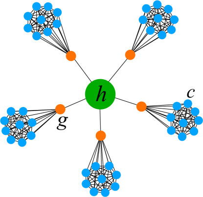
Figure SI.7: An example of star of cliques with $n=10$ and $m=5$.

The solution is

$$\begin{cases}\tau_{gh}=\frac{m^{2}(2n-1)((n-1)n+1)((n-1)n+3)(n(n+3)-2)-m(2n^{7}+n^{6}-15n^{5}+40n^{4}-52n^{3}+44n^{2}-24n+6)+n((n-3)n+1)(n-1)^{3}}{m^{2}(2n-1)(n(n+3)-2)+m(n(n(2n^{3}+3n-7)+6)-2)+n(n-1)^{3}},\\ \\ \tau_{hc}=\frac{m^{2}(n(n+3)-2)(2n^{5}-4n^{4}+10n^{3}-8n^{2}+5n-2)+m(-2n^{7}+n^{6}+7n^{5}-21n^{4}+24n^{3}-23n^{2}+16n-4)-(n-1)^{3}n^{2}(n+2)}{m^{2}(2n-1)(n(n+3)-2)+m(n(n(2n^{3}+3n-7)+6)-2)+n(n-1)^{3}},\\ \\ \tau_{cc}=\frac{m(n-1)(m(2n^{5}-4n^{4}+12n^{3}-5n^{2}+3n-2)+(n-1)n(5n^{2}+3)+2)}{m^{2}(2n-1)(n(n+3)-2)+m(n(n(2n^{3}+3n-7)+6)-2)+n(n-1)^{3}},\\ \\ \tau_{gc}=\frac{(n-1)(m^{2}(4n^{5}-8n^{4}+22n^{3}-15n^{2}+13n-6)+m(-2n^{5}+10n^{4}-13n^{3}+13n^{2}-12n+6)-(n-1)^{3}n)}{m^{2}(2n-1)(n(n+3)-2)+m(n(n(2n^{3}+3n-7)+6)-2)+n(n-1)^{3}},\\ \\ \tau_{gg^{\prime}}=\frac{m(m(n(n+3)-2)(2n^{6}-4n^{5}+10n^{4}-8n^{3}+3n^{2}+3n-2)-(n-2)(n-1)^{3}n^{2}(3n+1))}{n(m^{2}(2n-1)(n(n+3)-2)+m(n(n(2n^{3}+3n-7)+6)-2)+n(n-1)^{3})},\\ \\ \tau_{cc^{\prime}}=\frac{m(n(m(n(n+3)-2)(2n^{4}-4n^{3}+11n^{2}-7n+2)+n^{5}+10n^{4}-22n^{3}+14n^{2}-7n+8)-4)}{m^{2}(2n-1)(n(n+3)-2)+m(n(n(2n^{3}+3n-7)+6)-2)+n(n-1)^{3}},\\ \\ \tau_{gc^{\prime}}=\frac{m^{2}(n(n+3)-2)(2n^{5}-4n^{4}+11n^{3}-9n^{2}+5n-1)-m(n^{5}-11n^{4}+14n^{3}-10n^{2}+10n-6)(n-1)-(n-1)^{4}n}{m^{2}(2n-1)(n(n+3)-2)+m(n(n(2n^{3}+3n-7)+6)-2)+n(n-1)^{3}},\end{cases}$$ (79)

which gives

$$b^{*}(m,n)=\,\displaystyle\frac{\sum_{i=0,j=0}^{i=2,j=9}\theta_{ij}m^{i}n^{j}}{\sum_{i=0,j=0}^{i=2,j=8}\lambda_{ij}m^{i}n^{j}},$$ (80)

where the polynomial coefficients are given by matrices $\theta$ and $\lambda$:

$$\theta =\left[\begin{array}[]{rrrrrrrrrr}0&0&2&-5&4&-2&2&-1&0&0\\ 0&0&2&-9&22&-22&1&3&-5&0\\ 0&0&-8&26&-31&20&-9&8&0&2\end{array}\right],$$ (84)

$$\lambda =\left[\begin{array}[]{rrrrrrrrr}0&-4&18&-36&46&-42&24&-6&0\\ -8&32&-74&112&-99&55&-25&9&-4\\ 8&-44&88&-72&13&9&-4&2&2\end{array}\right].$$ (88)

For large $n$, we can expand the result as follows:

$$b^{*}=\left(\,\displaystyle\frac{m}{m-2}\right)n-\,\displaystyle\frac{(m+8)(m-1)}{(m-2)^{2}}+\left[\,\displaystyle\frac{14m^{4}+11m^{3}-14m^{2}-50m+44}{2m(m-2)^{3}}\right]\,\displaystyle\frac{1}{n}+O\left(\,\displaystyle\frac{1}{n^{2}}\right).$$ (89)

S3.H Connecting two cliques via a star

If we have two cliques of size $n$ and a star of size $m$ (that is, $m-1$ leafs and one hub), we can connect the hub of the star to one gate node from each clique. An example case with $n=20,m=5$ is depicted in Figure SI.8. We denote the hub of the star with $h$, its leafs with $\ell$, the gate nodes with $g$, and the non-gate nodes within the cliques with $c$. The remeeting times satisfy the following equations:

$$\begin{cases}\tau_{cc}=1+\frac{1}{n-1}\big{[}(n-3)\tau_{cc}+\tau_{cg}\big{]}\\ \tau_{cc^{\prime}}=1+\frac{1}{n-1}\big{[}(n-2)\tau_{cc^{\prime}}+\tau_{cg^{\prime}}\big{]}\\ \tau_{cg}=1+\frac{1}{2(n-1)}\big{[}(n-2)\tau_{cg}\big{]}+\frac{1}{2n}\big{[}(n-2)\tau_{cc}+\tau_{ch}\big{]}\\ \tau_{cg^{\prime}}=1+\frac{1}{2(n-1)}\big{[}(n-2)\tau_{cg^{\prime}}+\tau_{gg^{\prime}}\big{]}+\frac{1}{2n}\big{[}(n-1)\tau_{cc^{\prime}}+\tau_{ch}\big{]}\\ \tau_{ch}=1+\frac{1}{2(n-1)}\big{[}(n-2)\tau_{ch}+\tau_{gh}\big{]}+\frac{1}{2(m+1)}\big{[}(n-1)\tau_{c\ell}+\tau_{cg}+\tau_{cg^{\prime}}\big{]}\\ \tau_{c\ell}=1+\frac{1}{2(n-1)}\big{[}(n-2)\tau_{c\ell}+\tau_{g\ell}\big{]}+\frac{1}{2}\tau_{ch}\\ \tau_{gg^{\prime}}=1+\frac{1}{n}\big{[}(n-1)\tau_{cg^{\prime}}+\tau_{gh}\big{]}\\ \tau_{gh}=1+\frac{1}{2n}\big{[}(n-1)\tau_{ch}\big{]}+\frac{1}{2(m+1)}\big{[}(m-1)\tau_{g\ell}+\tau_{gg^{\prime}}\big{]}\\ \tau_{g\ell}=1+\frac{1}{2n}\big{[}(n-1)\tau_{c\ell}+\tau_{h\ell}\big{]}+\frac{1}{2}\tau_{gh}\\ \tau_{h\ell}=1+\frac{1}{2(m+1)}\big{[}(m-2)\tau_{\ell\ell}+2\tau_{g\ell}\big{]}\\ \tau_{\ell\ell}=1+\tau_{h\ell}\\ \end{cases}$$ (90)

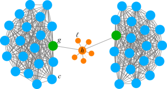
Figure SI.8: An example case of connecting cliques via a star with $n=20$ and $L=5$

The solution that we obtain is

$$b^{*}=\frac{\alpha}{\beta}$$ (91)

$$\alpha=\leavevmode\resizebox{411.93767pt}{}{$(m+1)n\bigg{[}2m^{4}n(6n^{2}-4n+1)(n(n+3)-2)+m^{3}(18n^{8}+36n^{7}+4n^{6}-87n^{5}+144n^{4}-131n^{3}+100n^{2}-48n+8)$}$$

$$+m^{2}n(6n^{9}-n^{8}+116n^{7}-78n^{6}+43n^{5}-270n^{4}+473n^{3}-363n^{2}+160n-34)$$

$$+m(34n^{10}-53n^{9}+202n^{8}-395n^{7}+448n^{6}-491n^{5}+527n^{4}-395n^{3}+163n^{2}-12n-8)$$

$$+2(n-1)^{2}(20n^{8}-11n^{7}+30n^{6}-25n^{5}+47n^{4}-42n^{3}+39n^{2}-16n)\bigg{]}$$ (92)

$$\beta=-2(80m^{4}+436m^{3}+1069m^{2}+1201m+428)n^{3}+2(m-1)(m+2)(3m+5)n^{10}$$

$$+(14m^{3}+68m^{2}+154m+174)n^{9}+(30m^{4}+18m^{3}-252m^{2}-488m-428)n^{8}$$

$$+(40m^{4}+318m^{3}+904m^{2}+1000m+606)n^{7}-4(41m^{4}+188m^{3}+330m^{2}+278m+132)n^{6}$$

$$+2(39m^{4}+143m^{3}+45m^{2}-55m+48)n^{5}+2(59m^{4}+310m^{3}+859m^{2}+931m+261)n^{4}$$

$$+4(20m^{4}+132m^{3}+329m^{2}+395m+165)n^{2}-8(2m^{4}+20m^{3}+53m^{2}+67m+31)n$$

$$+16(m+1)(m(m+2)+2)$$ (93)

Note that with $m=1$, which means that the star is only the hub with no leafs, so that the cliques are being connected via a single node, we recover Equation (75). For $1<m\ll n$, we can use the expansion:

$$b^{*}=\left(\,\displaystyle\frac{(m+4)(m+1)}{m^{2}+m-2}\right)n+\,\displaystyle\frac{(m+1)(15m^{4}+178m^{3}+579m^{2}+776m+452)}{2(3m+5)(m^{2}+m-2)^{2}}+O\left(\,\displaystyle\frac{1}{n}\right).$$ (94)

Note that in the main text, the number of leafs is denoted by $m$, whereas here the size of the star is denoted by $m$. Thus, to recover the result of the main text one must simply replace $m$ with $m+1$ in the above equation.

For the simple case of $m=2$, which means that the star is simply a dyad, and the cliques are being connected via a bridging node with a leaf attached to it, we get:

$$b^{*}\bigg{|}_{m=2}=\frac{9n}{2}-51+\frac{27585}{44n}+O\left(\,\displaystyle\frac{1}{n^{2}}\right)..$$ (95)

In the special case of $m=n$, we have:

$$b^{*}=\frac{\alpha}{\beta}$$ (96)

where the numerator is:

$$\alpha=\leavevmode\resizebox{390.25534pt}{}{$n^{2}(n+1)(6n^{11}+51n^{10}+139n^{9}+38n^{8}-267n^{7}+84n^{6}+127n^{5}-62n^{4}+57n^{3}-135n^{2}+130n-40),$}$$ (97)

and the denominator is:

$$\beta =6n^{13}+60n^{12}+124n^{11}+36n^{10}-94n^{9}-344n^{8}+44n^{7}$$

$$+288n^{6}+332n^{5}-724n^{4}+316n^{3}+172n^{2}-184n+32.$$ (98)

For large $n$, we can use the following expansion:

$$b^{*}=n-\frac{1}{2}+\frac{16}{n}+O\left(\,\displaystyle\frac{1}{n^{2}}\right).$$ (99)

S3.I Hierarchy of cliques

We can also connect communities in a hierarchical structure. We construct the hierarchical network by connecting a base node (denoted by $b$) to $q$ middle nodes (denoted by $m$), and connecting each middle node to a gate node (denoted by $g$) of a clique of size $n$. So there are $q^{2}$ cliques. We denote the non-gate nodes within cliques by $c$ (for ‘commoner’). An example case with $q=3$ and $n=5$ is illustrated in Figure SI.9.

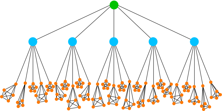
Figure SI.9: An example case of hierarchical connection of cliques with $q=3$ and $n=5$.

The remeeting times of interest are $\tau_{b,m}$ (between the base node and a middle node), $\tau_{b,g}$ (between the base node and a gate node), $\tau_{b,c}$ (between the base node and a commoner), $\tau_{m,g}$ (between a middle node and a gate node adjacent to it), $\tau_{m,g^{\prime}}$ (between a middle node and a gate node adjacent to another middle node), $\tau_{m,c}$ (between a middle node and a commoner of an adjacent clique), $\tau_{m,c^{\prime}}$ (between a middle node and a commoner of a clique adjacent to another middle node), $\tau_{m,m^{\prime}}$ (between two middle nodes), $\tau_{c,g}$ (between a commoner and a gate node in the same community), $\tau_{c,g^{\prime}}$ (between a commoner and the gate node of another community, the two communities being adjacent to the same middle node), $\tau_{c,g^{\prime\prime}}$ (between a commoner of a community and the gate node of another community, the two communities being adjacent to two distinct middle nodes), $\tau_{c,c^{\prime}}$ (between two commoners within the same community), $\tau_{c,c^{\prime\prime}}$ (between a commoner in one community and a commoner in another community, the two communities being adjacent to the same middle node), $\tau_{c,c^{\prime\prime\prime}}$ (between a commoner in one community and a commoner in another community, the two communities being adjacent to the distinct middle nodes), $\tau_{g,g^{\prime}}$ (between two gate nodes adjacent to the same middle node), $\tau_{g,g^{\prime\prime}}$ (between two gate nodes adjacent to two distinct middle nodes).

$$\begin{cases}\tau_{b,m}=\frac{(q-1)\tau_{m,m^{\prime}}}{2q}+\frac{q\tau_{b,g}}{2(q+1)}+1\\ \tau_{b,g}=\frac{(q-1)\tau_{m,g^{\prime}}+\tau_{m,g}}{2q}+\frac{(n-1)\tau_{b,c}+\tau_{b,m}}{2n}+1\\ \tau_{b,c}=\frac{(q-1)\tau_{m,c^{\prime}}+\tau_{m,c}}{2q}+\frac{(n-2)\tau_{b,c}+\tau_{b,g}}{2(n-1)}+1\\ \tau_{m,g}=\frac{(n-1)\tau_{m,c}}{2n}+\frac{(q-1)\tau_{g,g^{\prime}}+\tau_{b,g}}{2(q+1)}+1\\ \tau_{m,g^{\prime}}=\frac{(n-1)\tau_{m,c^{\prime}}+\tau_{m,m^{\prime}}}{2n}+\frac{q\tau_{g,g^{\prime\prime}}+\tau_{b,g}}{2(q+1)}+1\\ \tau_{m,c}=\frac{(n-2)\tau_{m,c}+\tau_{m,g}}{2(n-1)}+\frac{(q-1)\tau_{c,g^{\prime}}+\tau_{b,c}+\tau_{c,g}}{2(q+1)}+1\\ \tau_{m,c^{\prime}}=\frac{(n-2)\tau_{m,c^{\prime}}+\tau_{m,g^{\prime}}}{2(n-1)}+\frac{q\tau_{c,g^{\prime\prime}}+\tau_{b,c}}{2(q+1)}+1\\ \tau_{m,m^{\prime}}=\frac{q\tau_{m,g^{\prime}}+\tau_{b,m}}{\text{km}}+1\\ \tau_{c,g}=\frac{(n-2)\tau_{c,g}}{2(n-1)}+\frac{(n-2)\tau_{c,c^{\prime}}+\tau_{m,c}}{2n}+1\\ \tau_{c,g^{\prime}}=\frac{(n-2)\tau_{c,g^{\prime}}+\tau_{g,g^{\prime}}}{2(n-1)}+\frac{(n-1)\tau_{c,c^{\prime\prime}}+\tau_{m,c}}{2n}+1\\ \tau_{c,g^{\prime\prime}}=\frac{(n-2)\tau_{c,g^{\prime\prime}}+\tau_{g,g^{\prime\prime}}}{2(n-1)}+\frac{(n-1)\tau_{c,c^{\prime\prime\prime}}+\tau_{m,c^{\prime}}}{2n}+1\\ \tau_{g,g^{\prime}}=\frac{(n-1)\tau_{c,g^{\prime}}+\tau_{m,g}}{k_{g}}+1\\ \tau_{g,g^{\prime\prime}}=\frac{(n-1)\tau_{c,g^{\prime\prime}}+\tau_{m,g^{\prime}}}{k_{g}}+1\\ \tau_{c,c^{\prime}}=\frac{(n-3)\tau_{c,c^{\prime}}+\tau_{c,g}}{k_{c}}+1\\ \tau_{c,c^{\prime\prime}}=\frac{(n-2)\tau_{c,c^{\prime\prime}}+\tau_{c,g^{\prime}}}{k_{c}}+1\\ \tau_{c,c^{\prime\prime\prime}}=\frac{(n-2)\tau_{c,c^{\prime\prime\prime}}+\tau_{c,g^{\prime\prime}}}{k_{c}}+1.\end{cases}$$ (100)

Using these results we arrive at $b^{*}$. For the numerator, the For the numerator, the $i-j$ element of the following matrix yields the coefficient of $n^{i-1}q^{j-1}$ in the numerator:

(116)

and for the denominator we have:

(131)

For large $n$, we can use the following expansion:

$$b^{*}=\left[\frac{q^{2}\left(2q^{2}+q+1\right)}{q^{2}\left(2q^{2}+q+3\right)-6q-4}\right]n$$

$$+\frac{-16q^{11}-60q^{10}-152q^{9}-307q^{8}-689q^{7}-1105q^{6}-523q^{5}+827q^{4}+1226q^{3}+619q^{2}+136q+12}{(q+1)^{2}(4q+3)\Big{[}q\left(q\left(2q^{2}+q+3\right)-6\right)-4\Big{]}^{2}}$$

$$+O\left(\,\displaystyle\frac{1}{n}\right).$$ (132)

For example, for $q=2$, we have

$$b^{*}\bigg{|}_{q=2}=\,\displaystyle\frac{11}{9}n\bigg{[}1+O\left(\,\displaystyle\frac{1}{n}\right)\bigg{]}.$$ (133)

For $q=3$, we have

$$b^{*}\bigg{|}_{q=3}=\,\displaystyle\frac{99}{97}n\bigg{[}1+O\left(\,\displaystyle\frac{1}{n}\right)\bigg{]}.$$ (134)

The prefactor in the asymptotic expression becomes ${148/149}$ for $q=4$, and ${175/177}$ for $q=5$. As $q$ grows further, the prefactor approaches unity from below.

S3.J Ring of cliques

We assume $L$ cliques, each with $n$ nodes, situated on a ring via ‘gate’ nodes. Figure SI.10 shows an example of clique of rings with $L=5$ and $n=10$. We denote the gate nodes by $g$, and other nodes by $c$ ($c$ stands for commoner). The remeeting times that we need to obtain are $\tau_{gg}(x)$ (between two gate nodes separated by a distance $x$ on the ring), $\tau_{gc}(x)$ (between a gate node and a commoner in another community $x$ apart), and $\tau_{cc}(x)$ (between a commoner from one community and a commoner from another community $x$ apart).

The recurrence relations are:

$$\begin{cases}\text{for }x=2\ldots L-2:~{}&\begin{cases}\tau_{gg}(x)=1+\frac{1}{(n+1)}\bigg{[}\tau_{gg}(x-1)+\tau_{gg}(x+1)+(n-1)\tau_{gc}(x)\bigg{]}\\ \\ \leavevmode\resizebox{303.53267pt}{}{$\tau_{cg}(x)=1+\,\displaystyle\frac{1}{2(n+1)}\bigg{[}(n-1)\tau_{cc}(x)+\tau_{cg}(x+1)+\tau_{cg}(x-1)\bigg{]}+\,\displaystyle\frac{1}{2(n-1)}(n-2)\tau_{cc}(x)$}\\ \\ \tau_{cc}(x)=1+\,\displaystyle\frac{1}{n-1}\bigg{[}\tau_{cg}(x)+(n-2)\tau_{cc}(x)\bigg{]}\end{cases}\\ \\ \text{for }x<2:~{}&\begin{cases}\tau_{gg}(1)=1+\,\displaystyle\frac{1}{(n+1)}\bigg{[}\tau_{gg}(2)+(n-1)\tau_{cg}(1)\bigg{]}\\ \\ \leavevmode\resizebox{303.53267pt}{}{$\tau_{cg}(1)=1+\,\displaystyle\frac{1}{2(n+1)}\bigg{[}(n-1)\tau_{cc}(1)+\tau_{cg}(2)+\tau_{cg}(0)\bigg{]}+\,\displaystyle\frac{1}{2(n-1)}\bigg{[}(n-2)\tau_{cg}(1)+\tau_{gg}(1)\bigg{]}$}\\ \\ \leavevmode\resizebox{303.53267pt}{}{$\tau_{cg}(0)=1+\,\displaystyle\frac{1}{2(n+1)}\bigg{[}(n-2)\tau_{cc}(0)+2\tau_{cg}(1)\bigg{]}+\,\displaystyle\frac{1}{2(n-1)}(n-2)\tau_{cg}(0)$}\\ \\ \tau_{cc}(0)=1+\,\displaystyle\frac{1}{n-1}\bigg{[}\tau_{cg}(0)+(n-3)\tau_{cc}(0)\bigg{]}\\ \\ \tau_{cc}(1)=1+\,\displaystyle\frac{1}{n-1}\bigg{[}\tau_{cg}(1)+(n-2)\tau_{cc}(1)\bigg{]}.\end{cases}\end{cases}$$ (135)

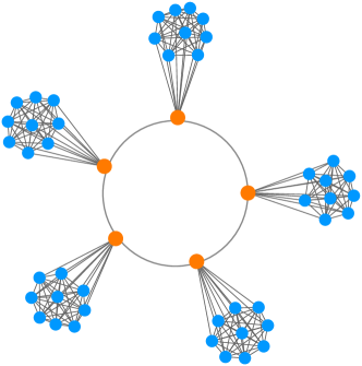
Figure SI.10: An example case of ring of cliques with $n=10$ and $L=5$

This is a system of linear difference equations with constant coefficients. Plugging in the ansatz $r^{x}+r^{L-x}$, we find that the characteristic equation for $r$ is given by

$$(r-1)^{2}\bigg{[}(n-1)r^{2}-n(n+1)r+(n-1)\bigg{]}=0.$$ (136)

There are four roots: $r=0$ has degeneracy 2, the third root is

$$R=\,\displaystyle\frac{n^{2}+n+\displaystyle\sqrt{[n(n-1)+2]~{}[n(n+3)-2]}}{2(n-1)},$$ (137)

and the fourth root is $1/R$.

The double degeneracy of root zero means that the particular solution to the nonhomogenous equation is quadratic in $x$. Thus we plug in the following form into the system of equations:

$$\begin{cases}\tau_{gg}(x)=A_{gg}x^{2}+B_{gg}x+C_{gg}+D_{gg}\big{(}R^{x}+R^{L-x}\big{)}\\ \tau_{cg}(x)=A_{cg}x^{2}+B_{cg}x+C_{cg}+D_{cg}\big{(}R^{x}+R^{L-x}\big{)}\\ \tau_{cc}(x)=A_{cc}x^{2}+B_{cc}x+C_{cc}+D_{cc}\big{(}R^{x}+R^{L-x}\big{)}\end{cases}$$ (138)

For brevity of notation, we define:

$$\xi\stackrel{{\scriptstyle\text{def}}}{{=}}\displaystyle\sqrt{[n(n-1)+2]~{}[n(n+3)-2]~{}}.$$ (139)

Using this along with the value of $R$ obtained above, we arrive at

$$A_{gg}=A_{cc}=A_{gc}=\frac{1}{2}\left(-n^{2}+n-2\right),$$

$$B_{gg}=B_{cc}=B_{gc}=\frac{1}{2}L((n-1)n+2),$$

$$D_{gg}=\leavevmode\resizebox{390.25534pt}{}{$-\,\displaystyle\frac{2^{L+1}(n-1)^{3}\left((L-1)n^{2}-Ln+2L+n\right)}{-2^{L+1}n\xi+2n\xi(2R)^{L}+(n-1)n((n-1)n+2)(2R)^{L}+2^{L}(n-1)n((n-1)n+2)-2^{L+1}\xi+2\xi(2R)^{L}}$}$$

$$D_{gc}=\leavevmode\resizebox{390.25534pt}{}{$\frac{2^{L+1}\left(n^{2}-1\right)\left((L-1)n^{2}-Ln+2L+n\right)}{-2^{L+1}n\xi+2n\xi(2R)^{L}+(n-1)n((n-1)n+2)(2R)^{L}+2^{L}(n-1)n((n-1)n+2)-2^{L+1}\xi+2\xi(2R)^{L}}$}$$

$$D_{cc}=(n-1)+D_{gc}.$$ (140)

The expressions for other variables are omitted for undue length. Using the solutions, we get the critical benefit to cost ratio:

$$b^{*}=\,\displaystyle\frac{\alpha}{\beta},$$ (141)

where the numerator is given by:

$$+R^{L}4^{L}\xi L\Big{(}2n^{17}+2n^{16}-12n^{15}-36n^{14}-140n^{13}-220n^{12}-488n^{11}-776n^{10}-678n^{9}$$

$$-1046n^{8}-892n^{7}-100n^{6}-256n^{5}+64n^{4}+544n^{3}+64n^{2}-128n\Big{)}$$

$$+R^{L}4^{L+1}\xi\Big{(}-2n^{16}-2^{L+1}n^{15}+2^{L+2}n^{14}-2^{L+2}n^{13}+39\ 2^{L+2}n^{12}+123\ 2^{L+2}n^{11}+99\ 2^{L+3}n^{10}+143\ 2^{L+3}n^{9}$$

$$+611\ 2^{L+1}n^{8}+379\ 2^{L+1}n^{7}+53\ 2^{L+2}n^{6}-41\ 2^{L+2}n^{5}-23\ 2^{L+4}n^{4}-15\ 2^{L+4}n^{3}+2^{L+5}n^{2}+2^{L+6}n\Big{)}$$

$$-2(n+1)^{2}R^{2L}4^{L}\Big{(}n^{16}+2n^{15}+8n^{14}+44n^{13}+44n^{12}+244n^{11}+256n^{10}+24n^{9}$$

$$+969n^{8}-782n^{7}+760n^{6}-468n^{5}-254n^{4}+280n^{3}-216n^{2}+144n-32\Big{)}$$

$$+2\xi R^{2L}4^{L}\leavevmode\resizebox{411.93767pt}{}{$\Big{(}-n^{16}-3n^{15}-12n^{14}-50n^{13}-106n^{12}-306n^{11}-508n^{10}-500n^{9}-605n^{8}g-343n^{7}+92n^{6}+78n^{5}+176n^{4}+116n^{3}-60n^{2}-16n\Big{)}$}$$

$$-2^{2L+1}(n+1)^{2}\Big{(}n^{16}-2n^{15}-16n^{14}+12n^{13}+20n^{12}+100n^{11}+248n^{10}+144n^{9}$$

$$+609n^{8}-154n^{7}+568n^{6}-556n^{5}+226n^{4}-200n^{3}-88n^{2}+144n-32\Big{)}$$

$$+2^{2L+1}\xi\Big{(}-n^{16}+n^{15}+16n^{14}+14n^{13}-26n^{12}-162n^{11}-364n^{10}-532n^{9}$$

$$-605n^{8}-499n^{7}-200^{6}+46n^{5}+128n^{4}+156n^{3}+28n^{2}-48n\Big{)},$$ (142)

and the denominator is given by:

$$\beta=\leavevmode\resizebox{390.25534pt}{}{$L2^{2L+1}R^{L}[(n-1)n+2]^{2}(n^{6}+n^{5}-7n^{4}-33n^{3}-46n^{2}-4n+24)(n^{8}+4n^{7}+2n^{6}+4n^{5}+11n^{4}-8n^{3}+8n^{2}-8n+2)$}$$

$$+L4^{L}R^{L}\xi\Big{(}\leavevmode\resizebox{368.57964pt}{}{$2n^{16}+4n^{15}-12n^{14}-56n^{13}-148n^{12}-248n^{11}-608n^{10}-832n^{9}-638n^{8}-1228n^{7}-868n^{6}$}$$

$$+368n^{6}-482n^{5}+18n^{4}+46n^{3}-204n^{2}+200n\Big{)}+L\xi 4^{L}R^{2L}\Big{(}-48+n^{16}+6n^{15}+22n^{14}+56n^{13}$$

$$-1566n^{4}+352n^{3}-96n^{2}+128n-32)+2^{2L+1}\xi\Big{(}-n^{16}+3\ n^{15}+16n^{14}-28n^{13}-40n^{12}+16n^{11}$$

$$-434n^{10}-389\ 2^{2L+1}n^{9}-475n^{8}-1023n^{7}-374n^{6}+6n^{5}+532n^{4}+60n^{3}+8n^{2}-48n\Big{)}.$$ (143)

For large $n$, this can be expanded to give:

$$b^{*}=\left(\,\displaystyle\frac{L}{L-2}\right)n-\,\displaystyle\frac{(L+1)^{2}-5}{(L-2)^{2}}+O\left(\,\displaystyle\frac{1}{n}\right)$$ (144)

S4 The Rich Club

What we call the rich club is a graph with extreme core-periphery structure. We consider a clique of size $N_{c}$ as the core graph, and $N_{p}$ peripheral nodes. Each peripheral nodes is connected to every core node. Peripheral nodes are not connected to one another. So the degree of each peripheral node is $N_{c}$, and the degree of each core node is ${N_{p}+(N_{c}-1)}$.

It is easy to show that natural selection does not favor cooperation in a rich-club network regardless of $b/c$.

This network comprises two sets of nodes: $m$ hubs and $N-m$ leafs. Each leaf is connected to every hub, and to no other leaf. Each hub is connected to every node in the network. In other words, there is a complete graph of $m$ nodes as a super-hub, and all the $N-m$ leaf nodes are connected to the super-hub. Denoting the hub nodes by $h$ and the leaf nodes by $ell$, we have

$$\begin{cases}\tau_{cp}=1+\,\displaystyle\frac{1}{2N_{c}}(N_{c}-1)\tau_{cc}+\,\displaystyle\frac{1}{2(N_{p}+N_{c}-1)}\Big{[}(m-1)\tau_{cp}+(n-m-1)\tau_{pp}\Big{]}\\ \tau_{pp}=1+\frac{1}{N_{c}}(N_{c}\tau_{cp})\\ \tau_{cc}=1+\,\displaystyle\frac{1}{(N_{p}+N_{c}-1)}\Big{[}(N_{c}-2)\tau_{pp}+(N_{p})\tau_{cp}\Big{]}\end{cases}.$$ (145)

Solving this system and finding $b^{*}$ is straightforward. Denoting the total number of nodes by $N$, we have

(146)

but can be simplified if we expand the solution for large $N$:

$$b^{*}=-\,\displaystyle\frac{2N}{3}\,\displaystyle\frac{2m-1}{m-1}+\frac{1}{18}\bigg{[}8m+39+\,\displaystyle\frac{20}{m-1}\bigg{]}+O(\,\displaystyle\frac{1}{N}).$$ (147)

Consistent with the results discussed previously, this diverges for $N_{c}=1$ (ordinary star), because the fraction has a pole at $N_{c}=1$. For any other combination of $N_{c}$ and $N_{p}$, we get a negative value for $b^{*}$.

Now suppose we have two rich-club graphs, one with $N_{c}$ core nodes and $N_{p}$ peripheral nodes, the other with $M_{c}$ core nodes and $M_{p}$ peripheral nodes. Suppose we connect them by attaching a core node from the first one and a core node in the second one. We denote these two nodes $g$, denoting ‘gate’. The remeeting times to obtain are $\tau_{p_{1},p_{1}^{\prime}}$ (between two peripheral nodes in the firs graph), $\tau_{p_{1},c_{1}}$ (between a peripheral node in the first graph and a non-gate core node in the first graph), $\tau_{p_{1},g_{1}}$ (between a peripheral node in the first graph and the gate node of the first graph), $\tau_{p_{1},p_{2}}$ (between a peripheral node in the first graph and a peripheral node in the second graph), $\tau_{p_{1},c_{2}}$ (between a peripheral node in the first graph and a core node in the second graph), $\tau_{p_{1},g_{2}}$ (between a peripheral node in the first graph and the gate node of the second graph), $\tau_{c_{1},c_{1}^{\prime}}$ (between two distinct core nodes in the first graph), $\tau_{c_{1},g_{1}}$ (between a non-gate core node in the first graph and the gate node of the first graph), $\tau_{c_{1},p_{2}}$ (between a core node in the first graph and the peripheral node in the second graph), $\tau_{c_{1},c_{2}}$ (between a non-gate core node in the first graph and a non-gate core no in the second graph), $\tau_{c_{1},g_{2}}$ (between a non-gate core node in the first graph and the gate node of the second graph), $\tau_{g_{1},p_{2}}$ (between the gate node of the first graph and a peripheral node in the second graph), $\tau_{g_{1},c_{2}}$ (between the gate node of the first graph and a non-gate core node of the second graph), $\tau_{g_{1},g_{2}}$ (between the two gate nodes), $\tau_{p_{2},p_{2}^{\prime}}$ (between two distinct peripheral nodes in the second graph), $\tau_{p_{2},c_{2}}$ (between a peripheral node in the second graph and a non-gate core node of the second graph), $\tau_{p_{2},g_{2}}$ (between a peripheral node in the second graph and the gate node of the second graph), $\tau_{c_{2},c_{2}^{\prime}}$ (between two distinct core nodes in the second graph), and $\tau_{c_{2},g_{2}}$ (between a non-gate core node of the second graph and the gate node of the second graph).

$$\begin{cases}\tau_{p_{1},p_{1}^{\prime}}=1+\frac{(N_{c}-1)\tau_{p_{1},c_{1}}+\tau_{p_{1},g_{1}}}{N_{c}}\\ \vspace{-2mm}\tau_{p_{1},c_{1}}=1+\frac{\tau_{c_{1},c_{1}}(N_{c}-2)+\tau_{c_{1},g_{1}}}{2N_{c}}+\frac{(N_{c}-2)\tau_{p_{1},c_{1}}+(N_{p}-1)\tau_{p_{1},p_{1}^{\prime}}+\tau_{p_{1},g_{1}}}{2(N_{c}+N_{p}-1)}\\ \vspace{-2mm}\tau_{p_{1},g_{1}}=1+\frac{\tau_{c_{1},g_{1}}(N_{c}-1)}{2N_{c}}+\frac{(N_{c}-1)\tau_{p_{1},c_{1}}+(N_{p}-1)\tau_{p_{1},p_{1}^{\prime}}+\tau_{p_{1},g_{2}}}{2(N_{c}+N_{p})}\\ \vspace{-2mm}\tau_{p_{1},p_{2}}=1+\frac{\tau_{c_{1},p_{2}}(N_{c}-1)+\tau_{g_{1},p_{2}}}{2N_{c}}+\frac{(M_{c}-1)\tau_{p_{1},c_{2}}+\tau_{p_{1},g_{2}}}{2M_{c}}\\ \vspace{-2mm}\tau_{p_{1},c_{2}}=1+\frac{\tau_{c_{1},c_{2}}(N_{c}-1)+\tau_{g_{1},c_{2}}}{2N_{c}}+\frac{(M_{c}-2)\tau_{p_{1},c_{2}}+M_{p}\tau_{p_{1},p_{2}}+\tau_{p_{1},g_{2}}}{2(M_{c}+M_{p}-1)}\\ \vspace{-2mm}\tau_{p_{1},g_{2}}=1+\frac{\tau_{c_{1},g_{2}}(N_{c}-1)+\tau_{g_{1},g_{2}}}{2N_{c}}+\frac{(M_{c}-1)\tau_{p_{1},c_{2}}+M_{p}\tau_{p_{1},p_{2}}+\tau_{p_{1},g_{1}}}{2(M_{c}+M_{p})}\\ \vspace{-2mm}\tau_{c_{1},c_{1}}=1+\frac{\tau_{c_{1},c_{1}}(N_{c}-3)+\tau_{c_{1},g_{1}}+N_{p}\tau_{p_{1},c_{1}}}{(N_{c}+N_{p}-1)}\\ \vspace{-2mm}\tau_{c_{1},g_{1}}=1+\frac{\tau_{c_{1},c_{1}}(N_{c}-2)+\tau_{c_{1},g_{2}}+N_{p}\tau_{p_{1},c_{1}}}{2(N_{c}+N_{p})}+\frac{\tau_{c_{1},g_{1}}(N_{c}-2)+N_{p}\tau_{p_{1},g_{1}}}{2(N_{c}+N_{p}-1)}\\ \vspace{-2mm}\tau_{c_{1},p_{2}}=1+\frac{\tau_{c_{1},c_{2}}(M_{c}-1)+\tau_{c_{1},g_{2}}}{2M_{c}}+\frac{\tau_{c_{1},p_{2}}(N_{c}-2)+\tau_{g_{1},p_{2}}+N_{p}\tau_{p_{1},p_{2}}}{2(N_{c}+N_{p}-1)}\\ \vspace{-2mm}\tau_{c_{1},c_{2}}=1+\frac{\tau_{c_{1},c_{2}}(M_{c}-2)+\tau_{c_{1},g_{2}}+\tau_{c_{1},p_{2}}M_{p}}{2(M_{c}+M_{p}-1)}+\frac{\tau_{c_{1},c_{2}}(N_{c}-2)+\tau_{g_{1},c_{2}}+N_{p}\tau_{p_{1},c_{2}}}{2(N_{c}+N_{p}-1)}\\ \vspace{-2mm}\tau_{c_{1},g_{2}}=1+\frac{\tau_{c_{1},c_{2}}(M_{c}-1)+\tau_{c_{1},g_{1}}+\tau_{c_{1},p_{2}}M_{p}}{2(M_{c}+M_{p})}+\frac{\tau_{c_{1},g_{2}}(N_{c}-2)+\tau_{g_{1},g_{2}}+N_{p}\tau_{p_{1},g_{2}}}{2(N_{c}+N_{p}-1)}\\ \vspace{-2mm}\tau_{g_{1},p_{2}}=1+\frac{\tau_{c_{1},p_{2}}(N_{c}-1)+N_{p}\tau_{p_{1},p_{2}}+\tau_{p_{2},g_{2}}}{2(N_{c}+N_{p})}+\frac{\tau_{g_{1},c_{2}}(M_{c}-1)+\tau_{g_{1},g_{2}}}{2M_{c}}\\ \vspace{-2mm}\tau_{g_{1},c_{2}}=1+\frac{\tau_{c_{1},c_{2}}(N_{c}-1)+\tau_{c_{2},g_{2}}+N_{p}\tau_{p_{1},c_{2}}}{2(N_{c}+N_{p})}+\frac{\tau_{g_{1},c_{2}}(M_{c}-2)+\tau_{g_{1},g_{2}}+\tau_{g_{1},p_{2}}M_{p}}{2(M_{c}+M_{p}-1)}\\ \vspace{-2mm}\tau_{g_{1},g_{2}}=1+\frac{\tau_{c_{1},g_{2}}(N_{c}-1)+N_{p}\tau_{p_{1},g_{2}}}{2(N_{c}+N_{p})}+\frac{\tau_{g_{1},c_{2}}(M_{c}-1)+\tau_{g_{1},p_{2}}M_{p}}{2(M_{c}+M_{p})}\\ \vspace{-2mm}\tau_{p_{2},p_{2}}=1+\frac{(M_{c}-1)\tau_{p_{2},c_{2}}+\tau_{p_{2},g_{2}}}{M_{c}}\\ \vspace{-2mm}\tau_{p_{2},c_{2}}=1+\frac{\tau_{c_{2},c_{2}}(M_{c}-2)+\tau_{c_{2},g_{2}}}{2M_{c}}+\frac{(M_{c}-2)\tau_{p_{2},c_{2}}+(M_{p}-1)\tau_{p_{2},p_{2}}+\tau_{p_{2},g_{2}}}{2(M_{c}+M_{p}-1)}\\ \vspace{-2mm}\tau_{p_{2},g_{2}}=1+\frac{\tau_{c_{2},g_{2}}(M_{c}-1)}{2M_{c}}+\frac{\tau_{g_{1},p_{2}}+(M_{c}-1)\tau_{p_{2},c_{2}}+(M_{p}-1)\tau_{p_{2},p_{2}}}{2(M_{c}+M_{p})}\\ \vspace{-2mm}\tau_{c_{2},c_{2}}=1+\frac{\tau_{c_{2},c_{2}}(M_{c}-3)+\tau_{c_{2},g_{2}}+M_{p}\tau_{p_{2},c_{2}}}{(M_{c}+M_{p}-1)}\\ \vspace{-2mm}\tau_{c_{2},g_{2}}=1+\frac{\tau_{c_{2},c_{2}}(M_{c}-2)+\tau_{g_{1},c_{2}}+M_{p}\tau_{p_{2},c_{2}}}{2(M_{c}+M_{p})}+\frac{\tau_{c_{2},g_{2}}(M_{c}-2)+M_{p}\tau_{p_{2},g_{2}}}{2(M_{c}+M_{p}-1)}\end{cases}$$ (148)

The solution is too lengthy to be presentable. Here we only provide the solution for the symmetric, case, where $M_{c}=N_{c}$ and $M_{p}=N_{p}$. We represent the result with two matrices for the polynomial coefficients of the numerator and the denominator. For the numerator, the $i-j$ element of the following matrix yields the coefficient of $N_{c}^{i-1}N_{p}^{j-1}$ in the numerator:

(168)

and for the denominator we have:

(186)

We can simplify the results in limiting cases. For large $N_{p}$, we can use the following expansion:

$$b^{*}=\left(4N_{c}-\frac{3}{2}\right)+\left[4N_{c}^{2}-\frac{47N_{c}}{4}-\frac{1}{4N_{c}}-\frac{45}{3N_{c}+2}+\frac{75}{4}\right]\,\displaystyle\frac{1}{N_{p}}+O\left(\,\displaystyle\frac{1}{N_{p}^{2}}\right).$$ (187)

In the limit as the number of peripheral nodes approaches infinity, the critical benefit to cost ratio only depends on the number of core nodes.

For example, we put $N_{c}=1$, we recover Equation (48), which pertains to two stars connected via hubs. If we set $N_{c}=2$, we get

$$b^{*}=\,\displaystyle\frac{13}{2}+\,\displaystyle\frac{11}{2N_{p}}+O\left(\,\displaystyle\frac{1}{N_{p}^{2}}\right),$$ (188)

that is, $b^{*}$ approaches $13/2$ in the limit as $N_{p}\rightarrow\infty$.

S5 The complete bipartite graph

A bipartite graph is one whose nodes can be divided into to disjoint subsets such that there is no link within either of them, and every link in the graph connects a node to one of the subsets to a node in the other. A complete bipartite graph is a bipartite graph in which each node in the first subset is connected to every node in the other subset. A star graph is an example of a complete bipartite graph with the first subset being a single node, and the second subset comprising all the leafs.

Suppose we have two subsets, with sizes $n_{x}$ and $n_{y}$. The remeeting times follow the following relations:

$$\begin{cases}\tau_{xx}=1+\tau_{xy}\\ \tau_{yy}=1+\tau_{xy}\\ \tau_{xy}=1+\frac{1}{2n_{y}}\big{[}(n_{y}-1)\tau_{yy}\big{]}+\frac{1}{2n_{x}}\big{[}(n_{x}-1)\tau_{xx}\big{]}\end{cases}$$ (189)

The solution is

$$\tau_{x}=\tau_{y}=\frac{4n_{x}n_{y}}{n_{x}+n_{y}}.$$ (190)

It is straightforward to check that if we insert these values into (8), the denominator becomes zero. An alternative approach is taken in Ref (19) of the main text.

Now suppose we have two identical complete bipartite graphs, each with $n_{x}$ and $n_{y}$ nodes as above. We connect one $x$ node of the first graph to one $x$ node of the second graph. So the degree of the two gate nodes are $n_{y}+1$. The degree of non-gate $x$ nodes are $n_{y}$, and the degree of $y$ nodes are $n_{x}$. An example case with $n_{x}=10$ and $n_{y}=5$ is illustrated in Figure SI.11. The remeeting times of interest are $\tau_{x,x^{\prime}}$ (between two non-gate $x$ nodes of the same graph), $\tau_{x,x^{\prime\prime}}$ (between a non-gate $x$ node of one graph and a non-gate $x$ node of the other graph), $\tau_{y,y^{\prime}}$ (between two $y$ nodes of the same graph), $\tau_{y,y^{\prime\prime}}$ (between an $y$ node of one graph and a $y$ node of other graph), $\tau_{x,y}$ (between a non-gate $x$ node of a graph and a $y$ node in the same graph), $\tau_{x,y^{\prime}}$ (between a non-gate $x$ node in one graph and a $y$ node in the other graph), $\tau_{g,x}$ (between the gate node of a graph and a non-gate $x$ node of the same graph), $\tau_{g,x^{\prime}}$ (between the gate node of a graph and a non-gate $x$ node of the other graph), $\tau_{g,y}$ (between the gate node of a graph and a non-gate $y$ node of the same graph), $\tau_{g,y^{\prime}}$ (between the gate node of a graph and a non-gate $x$ node of the other graph), and $\tau_{g,g^{\prime}}$ (between the two gate nodes),

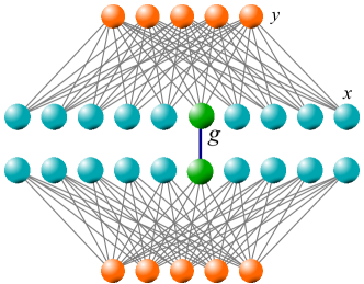
Figure SI.11: Connected complete bipartite graphs with $n_{x}=10$ and $n_{y}=5$

$$\begin{cases}\tau_{x,x^{\prime}}=1+\tau_{x,y}\\ \tau_{x,x^{\prime\prime}}=1+\tau_{x,y^{\prime}}\\ \tau_{y,y^{\prime}}=1+\frac{1}{n_{x}}\big{[}(n_{x}-1)\tau_{x,y}+\tau_{g,y}\big{]}\\ \tau_{y,y^{\prime\prime}}=1+\frac{1}{n_{x}}\big{[}(n_{x}-1)\tau_{x,y^{\prime}}+\tau_{g,y^{\prime}}\big{]}\\ \tau_{x,y}=1+\frac{1}{2n_{y}}\big{[}(n_{y}-1)\tau_{y,y^{\prime}}\big{]}+\frac{1}{2n_{x}}\big{[}(n_{x}-2)\tau_{x,x^{\prime}}+\tau_{g,x}\big{]}\\ \tau_{x,y^{\prime}}=1+\frac{1}{2}\tau_{y,y^{\prime\prime}}+\frac{1}{2}\big{[}(n_{x}-1)\tau_{x,x^{\prime\prime}}+\tau_{g,x^{\prime}}\big{]}\\ \tau_{g,x}=1+\frac{1}{2}\tau_{g,y}+\frac{1}{2(n_{y}+1)}\big{[}n_{y}\tau_{x,y}+\tau_{g,x^{\prime}}\big{]}\\ \tau_{g,x^{\prime}}=1+\frac{1}{2(n_{y}+1)}\big{[}n_{y}\tau_{x,y^{\prime}}+\tau_{g,x}\big{]}+\frac{1}{2}\tau_{g,y^{\prime}}\\ \tau_{g,y}=1+\frac{1}{2n_{x}}\big{[}(n_{x}-1)\tau_{g,x}\big{]}+\frac{1}{2(n_{y}+1)}\big{[}(n_{y}-1)\tau_{y,y^{\prime}}+\tau_{g,y^{\prime}}\big{]}\\ \tau_{g,y^{\prime}}=1+\frac{1}{2(n_{y}+1)}\big{[}n_{y}\tau_{y,y^{\prime\prime}}+\tau_{g,y}\big{]}+\frac{1}{2n_{x}}\big{[}(n_{x}-1)\tau_{g,x^{\prime}}+\tau_{g,g^{\prime}}\big{]}\\ \tau_{g,g^{\prime}}=1+\frac{1}{n_{y}+1}\big{[}n_{y}\tau_{g,y^{\prime}}\big{]}\end{cases}$$ (191)

The result is

$$b^{*}=\frac{\alpha}{\beta},$$ (192)

where the numerator is given by

$$\alpha=n_{1}(n_{2}+1)^{2}\bigg{[}2n_{1}^{4}n_{2}(n_{2}+1)(3n_{2}+2)(3n_{2}+4)(8n_{2}-1)$$

$$+n_{1}^{3}n_{2}(42n_{2}^{4}+474n_{2}^{3}+945n_{2}^{2}+623n_{2}+126)$$

$$-n_{1}^{2}(36n_{2}^{5}+235n_{2}^{4}+263n_{2}^{3}+24n_{2}^{2}-24n_{2}+12)$$

$$-n_{1}(3n_{2}+2)(6n_{2}^{3}+43n_{2}^{2}+25n_{2}-6)-2(n_{2}^{2}+9n_{2}+6)\bigg{]},$$ (193)

and the denominator is given by

$$\beta=4n_{1}^{5}n_{2}(n_{2}+1)(3n_{2}+2)(3n_{2}+4)(n_{2}(n_{2}+2)+2)$$

$$+2n_{1}^{4}(18n_{2}^{7}+102n_{2}^{6}+274n_{2}^{5}+435n_{2}^{4}+429n_{2}^{3}+316n_{2}^{2}+204n_{2}+64)$$

$$+n_{1}^{3}(24n2^{7}+84n2^{6}+20n2^{5}-155n2^{4}-240n2^{3}-467n2^{2}-538n2-192)$$

$$+n_{1}^{2}(8n_{2}^{6}-89n_{2}^{5}-531n_{2}^{4}-848n_{2}^{3}-412n_{2}^{2}+56n_{2}+60)$$

$$+n_{1}(34n_{2}^{5}+127n_{2}^{4}+138n_{2}^{3}+39n_{2}^{2}+2n_{2}+4)$$

$$+2n_{2}(n_{2}+1)(3n_{2}(n_{2}+3)+4)$$ (194)

For $n_{x}\ll n_{y}$, we can use the following expansion

$$b^{*}=4n_{x}-\frac{3}{2}+\left(14-\frac{1}{4n_{x}}+n_{x}-4n_{x}^{2}-\frac{45}{3n_{x}+2}\right)\,\displaystyle\frac{1}{n_{y}}+O\left(\,\displaystyle\frac{1}{n_{y}^{2}}\right).$$ (195)

Note that for $n_{x}=1$, we get the case of two stars connected via hubs, for which we showed that $b^{*}$ approaches $5/2$, as this new result reaffirms.

On the other hand, if we set $n_{y}=n_{y}=n$, we get

$$b^{*}\bigg{|}_{n_{x}=n_{y}=n}=2n-1+\,\displaystyle\frac{3}{n}+O\left(\,\displaystyle\frac{1}{n^{2}}\right)$$ (196)

S6 Conjoining scale-free networks

In the main text, Fig. 5, we presented the results for conjoining two ER networks, as well as two KE scale-free networks. In Figure SI.12, we present the same results of Fig. 5a of the main text (which pertained to conjoining of ER networks) but with $1/b^{*}$ instead of $b^{*}$. In Figure SI.13, we represent the results of Fig. 5c of the main text (which pertained to the conjoining of KE networks).

In this section, we present results for the same conjoining procedure applied to three additional scale-free network models that produce networks with heavy-tailed degree distributions that exhibit structural properties that actual social networks possess. The first model is the model of Holme and Kim [2] (HK), which produce networks with power-law degree distribution and high clustering. The second model is the Forest Fire (FF) model of Leskovec et al. [3], which in addition to the above properties, exhibits densification. The third model is Barthélemy’s spatial scale-free model (SSF) which combines preferential attachment with distance selection [4]. The fourth model is preferential attachment (PA) with initial attractiveness [5]. For the first thee models, we generate five networks of size 100 whose $b^{*}$ values equaled -1000, -500, -250, 250, 500, 1000 (within a 5% error margin). For the preferential attachment model, the generated graphs have typically better $b^{*}$ values and it we did not find an instance with negative $b^{*}$. The $b^{*}$ values of the two graphs under the PA model were 50, 100, 150, 200, and 250.

Then, for each pair of possible networks, we calculated the median $b^{*}$ of the composite network which results from creating a link between a node chosen from the first network and another chosen from the second network. We calculated the median value of all these $b^{*}$ values, and assigned it to that pair of networks. We repeated the same procedure for interconnections via one intermediary broker node as well. Figure SI.14 presents the results. Figure SI.15 presents the results using $1/b^{*}$ instead of $b^{*}$. In all cases, the $b^{*}$ of the composite network is better than those of the individual networks, and conjoining via one intermediary broker node is better than direct interconnection without an intermediary node.

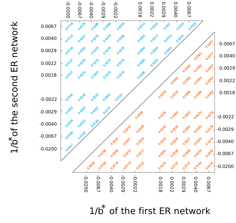
Figure SI.12: Conjoining two ER networks, the results being the same as those in Fig. 5a of the main text, but here we use $1/b^{*}$ to characterize the merit for cooperation instead of $b^{*}$.

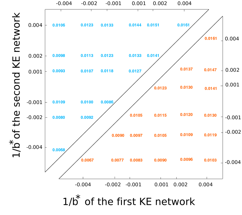
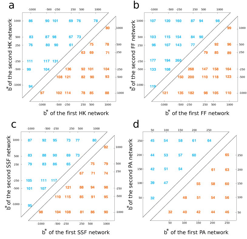
Figure SI.13: Conjoining two KE networks, the results being the same as those in Fig. 5c of the main text, but here we use $1/b^{*}$ to characterize the merit for cooperation instead of $b^{*}$.

Figure SI.14: Conjoining two scale-free networks. (a) The model of Holme and Kim, (b) The Forest-Fire model of Leskovec et al., (c) The Spatial Sale-free model of Barthelemy. (d) Preferential attachment model with initial attractiveness. In all cases, the blue numbers (upper triangle) represent the median $b^{*}$ value for interconnection of the two networks via an intermediary broker nodes, and the orange numbers (lower triangle) pertain to direct interconnections.

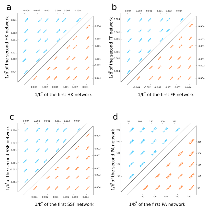
Figure SI.15: Same results as in Figure SI.14, but using $1/b^{*}$ instead of $b^{*}$.

S7 Community structure

We found in this paper that dense communities promote spite, and connecting them promotes cooperation. We demonstrated that connections with intermediary broker nodes are better at constructing composite networks that promote cooperation as compared to direct interconnections with no intermediary nodes.

Since sparsely interconnected cohesive groups is closely related to the notion of community structure in the network science literature, here we focus on two standard frameworks for producing networks with community structure: LFR benchmarks [6], and Stochastic Block Models [7]. Employing these two frameworks, in this section we investigate the role of community structure on the evolution of cooperation.

For the LFR benchmark, we used the publicly-available code that the authors of Ref. [6] have provided:
https://sites.google.com/site/santofortunato/inthepress2

We generated $10^{5}$ networks. For every input parameter, we selected a value from the possible range uniformly at random, and let the algorithm decide whether a network can be constructed from the given set of parameters. The network size is $N=100$. The mixing parameter was chosen uniformly at random in $[0,1]$, the maximum degree $k_{\text{max}}$ was chosen uniformly from the set of integers in the $(1,N]$ interval, the average degree was chosen uniformly from the set of integers in the $(1,k_{\text{max}}]$ interval, the degree exponent was uniformly chosen from the $[0,3]$ interval, the exponent for the community size distribution was chosen uniformly in the $[0,1]$ interval. We use network modularity [8] to quantify how strongly networks are divided into communities. Stronger division into communities pertains to higher values of modularity.

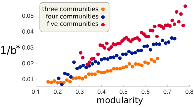
Figure SI.16: The effect of community structure on the evolution of cooperation for LFR benchmark graphs. Each marker represents the average value of data points falling in the corresponding bin of for modularity.

Fig. 6a shows the mean value of $1/b^{*}$ for different values of modularity. We plotted $1/b^{*}$ instead of $b^{*}$ merely because the patterns were visually better discernible. As modularity increases, $b^{*}$ decreases. The number of communities also affects $b^{*}$. For fixed size and given modularity, greater number of communities leads to less $b^{*}$, hence more conduciveness to the evolution of cooperation.

Stochastic Block Models (SBM) is another standard modeling framework for generating networks with community structure and also for inferring community structure [7]. This model simply involves two parameters: $P_{\text{within}}$ (the within-community link probability) and $P_{\text{between}}$ (the between-community link probability). For fixed network size $N=100$, we generated $10^{6}$ networks. Both $P_{\text{within}}$ and $P_{\text{between}}$ are selected uniformly at random from the interval $[0,1]$. Figure SI.17 depicts $1/b^{*}$ in terms of modularity. Consistent with the above results, higher modularity leads to lower values of $b^{*}$. Similar to the case of LFR, we plotted $1/b^{*}$ instead of $b^{*}$ simply because the patterns were visually better discernible

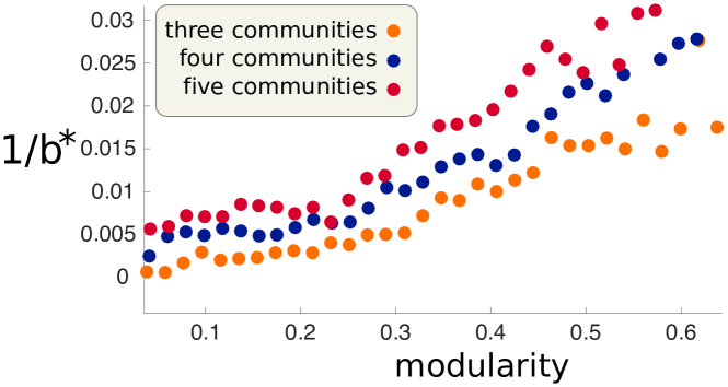
Figure SI.17: The effect of community structure on the evolution of cooperation for SBM benchmark graphs. Each marker represents the average value of data points falling in the corresponding bin of for modularity.

The second experiment on SBMs that we report is to investigate how $b^{*}$ depends on $P_{\text{within}}$ and $P_{\text{between}}$ . For the range $P_{\text{within}}\in[0.3,0.7]$ and $P_{\text{between}}\in(0,0.15]$, we plotted the expected value of $b^{*}$ averaged over $10^{4}$ realizations. We consider the cases of two, three, and four communities, each with size 100. The results are depicted in Figure SI.18. We find that for dense communities (which, as shown previously, support spite individually), sparse interconnections correspond to lower values of $b^{*}$. The results demonstrate that adding too many interconnections between the communities are not beneficial.

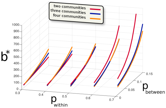
Figure SI.18: Results for SBM networks. When the communities have small within-community density, $b^{*}$ grows slowly by adding between-community links, as compared to dense communities. Moreover, the greater the number of communities are, this increase with between-community link density becomes steeper: For $P_{\text{within}}=0.3$, the curve pertaining to four communities has the highest $b^{*}$, but for $P_{\text{within}}=0.7$, the trend is reversed and the curve for two communities has the highest $b^{*}$ and the steepest increase with $P_{\text{between}}$.

S8 Robustness analysis

The above-considered topologies were ideal types amenable to exact analytical treatment. More realistic scenarios of course involve more randomness. We test if the above-considered topologies still produce reasonably-low values of $b^{*}$ in presence of noise. That is, do topologies close to those we considered possess fairly similar values of $b^{*}$ as we calculated? or do a small amount of structural noise vary the results markedly?

For fair comparison, we retain the number of links (so that density would be intact), and rewire each link with probability $p$, and then calculate the ratio of the $b^{*}$ of the rewired network to that of the original network. Since there are many ways to perform the rewiring, we consider the median value of the said ratio for given rewiring probability. Figure SI.19 presents the median ratio of $b^{*}$ to that of the original network as a function of the rewiring probability $p$ for the topologies considered above. In all cases, the distribution of this ratio is fairly close to unity. This demonstrates that in the presence noise, the noisy networks still exhibit the cooperative merit of the original composite networks.

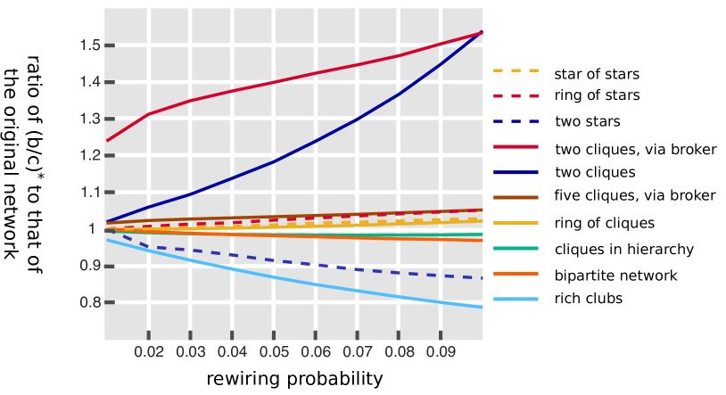
Figure SI.19: The robustness of the presented $b^{*}$ values for the structures discussed, as a function of the rewiring probability

S9 Simulation results

In addition to the robustness checks performed above, we also present simulation results for confirming the accuracy of the reported results for different topologies. Figure SI.20 presents the results for conjoining two stars each with 50 leaves, whose hubs are connected via a chain of zero, one, or two intermediary nodes (three cases depicted together). The vertical axis is the fixation probability times network size $N$. The dashed vertical purple line marks the theoretical prediction, that is, the value of $b^{*}$ at which the value of fixation probability times $N$ equals one. The markers represent simulation results for different values of $b$. The simulation results closely agree with the theoretical predictions. Figure SI.21 depicts the results for imperfect star of stars, Figure SI.22 for star of stars, and Figure SI.23 for ring of stars. Figure SI.24 depicts the results for the star of cliques, Figure SI.25 for conjoining to cliques via a star as described in Section S3.H, Figure SI.26 for ring of cliques, and Figure SI.33 for hierarchy of cliques as discussed in Section S3.I. Finally, Figure SI.28 presents the results for conjoining two rich clubs and Figure SI.29 pertains to the conjoining of two complete bipartite graphs. In all cases, the selection strengths for simulations is 0.01. The results are calculated over $10^{6}$ Monte Carlo trials. That is, for each network, we run $10^{6}$ trials in which we take a network in which every node is a defector, we select one node uniformly at random, we make it a cooperator, and initiate the dynamics according to the game and update mechanisms described in the paper. The fraction of trials that terminate in an all-C state is the fixation probability. The value of $c$ is set to 1 and the test values of $b$ are $0.9,0.95,1,1.05,$ and 1.1 of the theoretically-predicted $b^{*}$, so that the crossover can be visually observed from the figure with convenience.

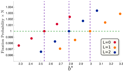
Figure SI.20: Simulation results for conjoining two stars, each with 50 leaves. Hubs are connected via zero, one, and two intermediary nodes.

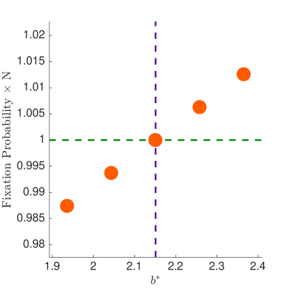
Figure SI.21: Simulation results for the imperfect star of stars: for a star graph with 15 leaves, we select five leaf nodes and to each of them connect 10 new leaf nodes. The theoretical prediction is $b^{*}\approx 2.15$.

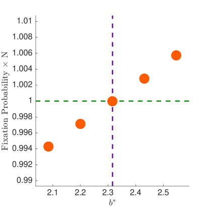
Figure SI.22: Simulation results for star of stars: We start from a star graph with 5 leaves, and to each leaf node we attach 5 new nodes. The theoretical prediction is $b^{*}\approx 2.32$.

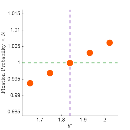
Figure SI.23: Simulation results for the ring of five stars, each with 20 leaf nodes. The theoretical prediction is $b^{*}\approx 1.84$. It is notable that the average degree is 2, and $b^{*}<2$. This is one of the superpromoter graphs discussed in the text.

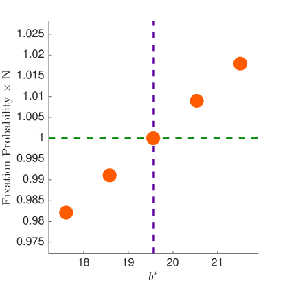
Figure SI.24: Simulation results for the star of cliques: four cliques, each of size 10, connected to a single broker node. The theoretical prediction is $b^{*}\approx 19.56$

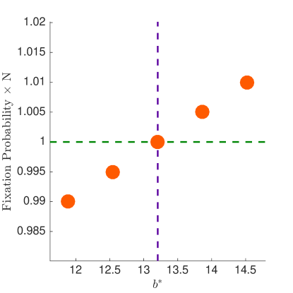
Figure SI.25: Simulation results for the conjoining of two cliques via a star graph. Two cliques of size 10, connected via a broker node, with four leaf nodes connected to the broker node. The theoretical prediction is $b^{*}\approx 13.21$.

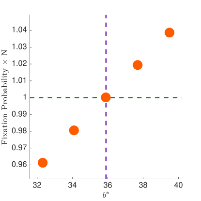
Figure SI.26: Simulation results for the ring of cliques: four cliques, each with size 20. The theoretical prediction is $b^{*}\approx 35.90$.

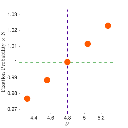
Figure SI.27: Simulation results for hierarchy of cliques, identical to the graph illustrated in Figure SI.9. The theoretical prediction is $b^{*}\approx 4.80$.

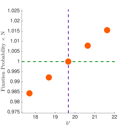
Figure SI.28: Simulation results for conjoining two rich clubs, each with 50 peripheral nodes and 5 core nodes. The theoretical prediction is $b^{*}\approx 19.66$.

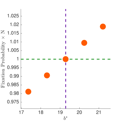
Figure SI.29: Simulation results for conjoining two complete bipartite graphs, each consisting of two sets of 10 nodes. The theoretical prediction is $b^{*}\approx 19.29$.

S10 Imitation updating

In addition to the DB updating considered in the main text, here we also provide the solution for imitation (IM) updating, in which each node also has the option of not updating its strategy at all (equivalently, copies its own strategy).

DB and IM updating can both be considered special cases of a general process, which we now describe. The population structure is defined by two sets of probabilities: the replacement probability $p_{xy}$ and the interaction probability $\tilde{p}_{xy}$. At each time-step, each individual $x$ interacts with other individuals $y$ with probability (or frequency) $\tilde{p}_{xy}$, receiving an expected payoff of $f_{x}$. This payoff is rescaled to $F_{x}=1+\delta f_{x}$, where $\delta>0$ represents the strength of selection. Then, an individual is chosen, uniformly at random, to update its strategy. The probability that individual $x$ imitates individual $y$ is proportional to $p_{xy}F_{y}$.

For DB updating on an unweighted, undirected graph, the replacement and interaction probabilities are the same:

$$p_{xy}=\tilde{p}_{xy}=\begin{cases}\frac{1}{k_{x}}&\text{ $y\in\mathcal{N}_{x}$}\\ 0&\text{otherwise}\end{cases}$$ (197)

For IM updating, the interaction probabilities $\tilde{p}_{xy}$ are again given by Eq. (197), but the replacement probabilities are instead given by

$$p_{xy}=\begin{cases}\frac{1}{k_{x}+1}&\text{if $y=x$ or $y\in\mathcal{N}_{x}$}\\ 0&\text{otherwise}\end{cases}$$ (198)

This reflects the fact that in IM updating, an individual can “imitate” itself (i.e. choose not to change its strategy).

We now provide a general derivation, valid for both DB and IM updating, of the conditions for cooperation to be favored under weak selection. More explicit details can be found in [1]. We represent the population state by a binary vector $\mathbf{s}=(s_{1},\ldots,s_{N})$, where $s_{x}=1$ if $x$ is a (C)ooperator and $s_{x}=0$ if vertex $x$ is a (D)efector. For the donation game

$$\bordermatrix{&\mathrm{C}&\mathrm{D}\cr\mathrm{C}&b-c&-c\cr\mathrm{D}&b&0},$$ (199)

the payoff to vertex $x$ can be expressed as

$$f_{x}(\mathbf{s})=-cs_{x}+b\sum_{y}\tilde{p}_{xy}s_{y}.$$ (200)

We require some notation for random walks. Consider a random walk starting at vertex $x$ that takes $m$ steps according to the replacement probabilities $p$, followed by $n$ steps according to interaction probabilities $\tilde{p}$. We denote by $p_{xy}^{(m,n)}$ the probability that such a walk terminates at vertex $y$. We let $\pi_{x}$ denote the stationary probability of vertex $x$ for random walks using the replacement probabilities $p$. These stationary probabilities are given by

$$\pi_{x}=\begin{cases}\displaystyle\frac{k_{x}}{\sum_{y}k_{y}}&\text{DB updating}\\[14.22636pt] \displaystyle\frac{k_{x}+1}{\sum_{y}(k_{y}+1)}&\text{IM updating}\end{cases}$$ (201)

The stationary probability $\pi_{x}$ can also be understood as the reproductive value (RV) of vertex $x$ [9]. Since random walks on undirected graphs are reversible (e.g. [10]), we have the reversibility property $\pi_{x}p_{xy}=\pi_{y}p_{yx}$, and more generally, $\pi_{x}p_{xy}^{(m,0)}=\pi_{y}p_{yx}^{(m,0)}$, valid for all vertices $x,y$ and all $m\geq 0$.

We study selection using the RV-weighted frequency $\hat{s}=\sum_{x}\pi_{x}s_{x}$. We denote expected change in $\hat{s}$ over a single time-step by $D(\mathbf{s})$, which can be calculated as

$$D(\mathbf{s}) =\frac{1}{N}\sum_{x}s_{x}\left(-\pi_{x}+\sum_{y}\pi_{y}\frac{F_{x}(\mathbf{s})p_{yx}}{\sum_{z}F_{z}(\mathbf{s})p_{yz}}\right)$$

$$=\frac{1}{N}\sum_{x}s_{x}\left(-\pi_{x}+\sum_{y}\pi_{y}\left(p_{yx}+\delta\left(f_{x}(\mathbf{s})p_{yx}-\sum_{z}f_{z}(\mathbf{s})p_{yz}\right)\right)\right)+\mathcal{O}(\delta^{2})$$

$$=\frac{\delta}{N}\sum_{x}\pi_{x}s_{x}\left(f_{x}^{(0,0)}(\mathbf{s})-f_{x}^{(2,0)}(\mathbf{s})\right)+\mathcal{O}(\delta^{2})$$

$$=\frac{\delta}{N}\sum_{x}\pi_{x}s_{x}\left(-c\left(s_{x}^{(0,0)}-s_{x}^{(2,0)}\right)+b\left(s_{x}^{(0,1)}-s_{x}^{(2,1)}\right)\right)+\mathcal{O}(\delta^{2}).$$

Above, we have made use of the reversibility property $\pi_{y}p_{yx}=\pi_{x}p_{xy}$ and we have introduced the notation

$$f_{x}^{(n,m)}=\sum_{y}p_{xy}^{(n,m)}f_{y},\qquad s_{x}^{(n,m)}=\sum_{y}p_{xy}^{(n,m)}s_{y}.$$

We define $D^{\prime}(\mathbf{s})$ to be the $\delta$-derivative of $D(\mathbf{s})$ at $\delta=0$:

$$D^{\prime}(\mathbf{s})=\frac{1}{N}\sum_{x}\pi_{x}s_{x}\left(-c\left(s_{x}^{(0,0)}-s_{x}^{(2,0)}\right)+b\left(s_{x}^{(0,1)}-s_{x}^{(2,1)}\right)\right).$$ (202)

[11] showed that the fixation probability of cooperators under weak selection can be expressed as

$$\rho_{\mathrm{C}}=\frac{1}{N}+\delta\langle D^{\prime}\rangle+\mathcal{O}(\delta^{2}),$$ (203)

where $\langle\;\rangle$ denotes an expectation over states arising under neutral drift, from an initial state with a single cooperator placed at a uniformly chosen random vertex. It follows that cooperation is favored under weak selection if and only if $\langle D^{\prime}\rangle>0$.

We can calculate $\langle D^{\prime}\rangle$ using the method of coalescing random walks [12, 13, 14, 11]. Consider a process involving two random walkers, initially located at vertices $x$ and $y$. At each time-step, one of the two walkers is chosen to take a step, using the step probabilities for replacement. The coalescence time $\tau_{xy}$ is defined as the expected time to until the two walkers meet. Coalescence times satisfy the recurrence relation

$$\tau_{xy}=\tau_{yx}=(1-\delta_{xy})\left[1+\sum_{z}(p_{xz}\tau_{zy}+p_{yz}\tau_{xz})\right]$$ (204)

Duality between CRW’s and the voter model [12, 14] implies that $\tau_{xy}$ is proportional to the expected time since $x$ and $y$ diverged from their most recent common ancestor. Using this duality, [1] obtain the identity

$$\left\langle s_{x}s_{y}-s_{z}s_{w}\right\rangle=\frac{\tau_{zw}-\tau_{xy}}{2}.$$ (205)

We introduce the notation

$$\tau^{(n,m)}=\sum_{x,y}\pi_{x}p_{xy}^{(n,m)}\tau_{xy}.$$ (206)

Then substituting Eqs. (202) and (205) into Eq. (203) we obtain the fixation probability of cooperation:

$$\rho_{\mathrm{C}}=\frac{1}{N}+\frac{\delta}{2N}\Big{(}-c\tau^{(2,0)}+b\left(\tau^{(2,1)}-\tau^{(0,1)}\right)\Big{)}+\mathcal{O}(\delta^{2}).$$

Cooperation is therefore favored under weak selection if and only if

$$-c\tau^{(2,0)}+b\left(\tau^{(2,1)}-\tau^{(0,1)}\right)>0.$$

[1] show that this condition implies both $\rho_{\mathrm{C}}>1/N$ and $\rho_{\mathrm{D}}<1/N$ under weak selection. The critical benefit-cost ratio is given by

$$b^{*}=\frac{\tau^{(2,0)}}{\tau^{(2,1)}-\tau^{(0,1)}}.$$ (207)

For DB updating (which we considered so far), since the replacement and interaction probabilities coincide, we can write the critical benefit-cost ratio more simply as

$$b^{*}=\frac{\tau^{(2)}}{\tau^{(3)}-\tau^{(1)}},$$ (208)

where $\tau^{(n)}=\sum_{x}\pi_{x}p_{xy}^{(n)}\tau_{xy}$. Eq. (204) leads to a recurrence for $\tau^{(n)}$:

$$\tau^{(n+1)}=\tau^{(n)}+\sum_{x}\pi_{x}p_{xx}^{(n)}\tau_{x}-1,$$ (209)

where $\tau_{x}=1+\sum_{y}p_{xy}\tau_{xy}$ is the remeeting time for two random walks from $x$. In particular (assuming the graph has no self-loops), we have

$$\tau^{(0)} =0$$ (210a)

$$\tau^{(1)} =\sum_{x}\pi_{x}\tau_{x}-1$$ (210b)

$$\tau^{(2)} =\sum_{x}\pi_{x}\tau_{x}-2$$ (210c)

$$\tau^{(3)} =\sum_{x}\pi_{x}\tau_{x}\left(1+p_{x}\right)-3.$$ (210d)

Above, $p_{x}=p_{xx}^{(2)}$ is the probability that a two-step random walk from $x$ returns to $x$. Using Eq. (210), we can rewrite the critical benefit-cost ratio in Eq. (211) as

$$b^{*} =\frac{\sum_{x}\pi_{x}\tau_{x}-2}{\sum_{x}\pi_{x}\tau_{x}p_{x}-2}=\frac{\sum_{x}k_{x}\tau_{x}-2N\bar{k}}{\sum_{x}k_{x}\tau_{x}p_{x}-2N\bar{k}}$$ (211)

In the case of IM updating, substituting from Eqs. (198), (201), and (206) into Eq. (207) gives the critical benefit-cost ratio for IM:

$$b^{*}=\frac{\sum_{x,y,z}(k_{x}+1)p_{xy}p_{yz}\tau_{xz}}{\sum_{x,y,z,w}(k_{x}+1)p_{xy}p_{yz}\tilde{p}_{zw}\tau_{xw}-\sum_{x,y}(k_{x}+1)p_{xy}\tau_{xy}}.$$

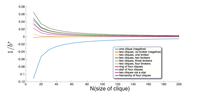
Figure SI.30: IM updating for conjoining cliques

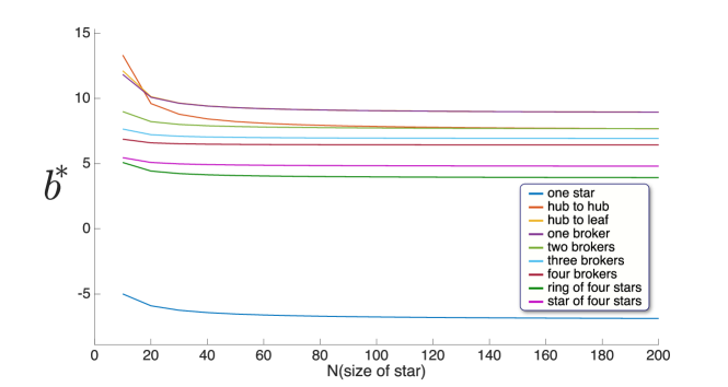
Figure SI.31: IM updating for conjoining stars

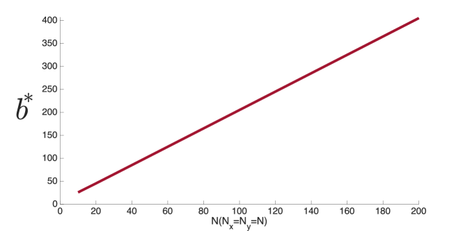
Figure SI.32: IM updating for conjoining complete bipartite networks

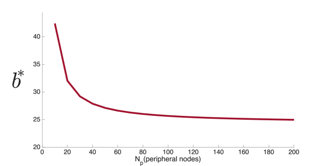
Figure SI.33: IM updating for conjoining rich clubs

S11 Summary of the results

The summary of the results for the real social network data sets (as discussed in main text) is presented in Table SI.1. For the high school network, division to both two and three communities returned reasonable groupings, so we reported results for both.

TABLE SI.1: results for real social network data sets

Network	N	m	bc	BC
fourth grade	24	2	-11,-39	41
fifth grade	22	2	-23,-47	19
high school	37	2	10,18	7.9
		3	10,-9,-151
zachary club	34	2	14.5,11.5	7.5

A condensed summary for the limiting behavior of $(b/c)^{*}$ for more notable topologies is presented in Table SI.2. A more comprehensive summary of the limiting behaviors of the conjoined graphs is presented in Table SI.3.

TABLE SI.2: Limiting behavior of results for notable topologies

Graph	$\left(\frac{b}{c}\right)^{\ast}$
Star	Inf
Star of Stars	$2$
Two Stars	$\frac{5}{2},3$
Ring of Stars	$\frac{3}{2}$
Clique	$-(N-1)$
Conjoined Cliques	$N^{2}$
Star of Cliques	$N$
Hierarchy of Cliques	$N$
Ring of Cliques	$N$
The Rich Club	$-N$
Conjoined Rich Clubs	$N_{c}$
Complete Bipartite	Inf
Conjoined Complete Bipartites	$2N$

TABLE SI.3: Summary of the limiting behavior of the $(b/c)^{*}$ of conjoined networks.

Graph	Parameters	Limit/Special case	$\left(\dfrac{b}{c}\right)^{\ast}$
Star	$n$ leaf nodes	N/A	Inf
Extended Star	two layers, each $n$ nodes	$n\to\infty$	$\dfrac{28}{11}\approx 2.55$
3-Layer Extended Star	three layers, each $n$ nodes	$n\to\infty$	$\dfrac{106940}{41723}\approx 2.56$
Imperfect Extended Star	Layer one $n$ nodes, Layer two $n_{g}$ nodes	$n_{g}\ll n$	$\dfrac{34}{89n_{g}}n\approx\dfrac{0.38}{n_{g}}n$
Star of Stars	$n$ leaf nodes, each connected to $n_{d}$ nodes	$n\ll n_{d}$	$\left(2+\dfrac{1}{n-1}\right)+\left(\dfrac{1}{2}+\dfrac{1}{1-n}\right)\dfrac{1}{n_{d}}$
Imperfect Star of Stars	$n$ leaf nodes, $n_{g}$ of them connected to $n_{d}$ nodes	$n_{g}\ll n\ll n_{d}$	$\dfrac{3}{2}+\dfrac{1}{2(n_{g}-1)}$
Two Stars: Hub to Leaf	Two stars, each with $n$ leaf nodes	$n\to\infty$	$\dfrac{5}{2}$
Two Stars: Leaf to Leaf	Two stars, each with $n$ leaf nodes	$n\to\infty$	$3$
Ring of Stars	$L$ stars, each with $n$ leaf nodes	$n\to\infty$	$\dfrac{3L-1}{2L-2}$
Clique	$n$ nodes	N/A	$-(n-1)$
Conjoined Cliques	two cliques, each with $n$ nodes	$n\to\infty$	$n^{2}$
Star of Cliques	$m$ cliques, each with $n$ nodes	$n\to\infty$	$\left(\dfrac{m}{m-2}\right)n-\dfrac{(m+8)(m-1)}{(m-2)^{2}}$
Connecting Two Cliques via a Star	two cliques of size $n$ connecting via a star of size $m$	$m=n,n\to\infty$	$n-\dfrac{1}{2}$
Hierarchy of Cliques	$q^{2}$ cliques of size $n$, at the bottom layer, connected to the base node via $q$ middle nodes	$n\to\infty$	$\left[\dfrac{q^{2}(2q^{2}+q+1)}{q^{2}(2q^{2}+q+3)-6q-4}\right]n$
Ring of Cliques	$L$ cliques of size $n$	$n\to\infty$	$\left(\dfrac{L}{L-2}\right)n-\dfrac{(L+1)^{2}-5}{(L-2)^{2}}$
The Rich Club	$N_{c}$ core and $N_{p}=N-N_{c}$ peripheral nodes	$N\to\infty$	$-\dfrac{2N}{3}\dfrac{2N_{c}-1}{N_{c}-1}+\dfrac{1}{18}\big{[}8N_{c}+39+\dfrac{20}{N_{c}-1}\big{]}$
Conjoined Rich Clubs	two rich clubs, each with $N_{c}$ core and $N_{p}$ peripheral nodes	$N_{p}\to\infty$	$4N_{c}-\frac{3}{2}$
Complete Bipartite	two subsets of nodes with sizes $n_{x}$ and $n_{y}$	N/A	Inf
Conjoined Complete Bipartite Graphs	two identical complete bipartite graphs with sizes $n_{x}$ and $n_{y}$	$n_{x}=n_{y}=n\to\infty$	$2n-1$

References

- [1] Nowak, M. A. Five rules for the evolution of cooperation. Science 314, 1560–1563 (2006).
- [2] Simpson, B. & Willer, R. Beyond altruism: Sociological foundations of cooperation and prosocial behavior. Annual Review of Sociology 41, 43–63 (2015).
- [3] Jordan, J. J., Rand, D. G., Arbesman, S., Fowler, J. H. & Christakis, N. A. Contagion of cooperation in static and fluid social networks. PloS one 8, e66199 (2013).
- [4] Rand, D. G., Nowak, M. A., Fowler, J. H. & Christakis, N. A. Static network structure can stabilize human cooperation. Proceedings of the National Academy of Sciences 111, 17093–17098 (2014).
- [5] Hauert, C. & Doebeli, M. Spatial structure often inhibits the evolution of cooperation in the snowdrift game. Nature 428, 643 (2004).
- [6] Lieberman, E., Hauert, C. & Nowak, M. A. Evolutionary dynamics on graphs. Nature 433, 312–316 (2005).
- [7] Ohtsuki, H., Hauert, C., Lieberman, E. & Nowak, M. A. A simple rule for the evolution of cooperation on graphs and social networks. Nature 441, 502–505 (2006).
- [8] Szabó, G. & Fath, G. Evolutionary games on graphs. Physics Reports 446, 97–216 (2007).
- [9] Débarre, F., Hauert, C. & Doebeli, M. Social evolution in structured populations. Nature Communications 5, 3409 (2014).
- [10] Allen, B. et al. Evolutionary dynamics on any population structure. Nature 544, 227–230 (2017).
- [11] Centola, D. The spread of behavior in an online social network experiment. Science 329, 1194–1197 (2010).
- [12] Centola, D. & Macy, M. Complex contagions and the weakness of long ties. American Journal of Sociology 113, 702–734 (2007).
- [13] Nowak, M. A. & May, R. M. Evolutionary games and spatial chaos. Nature 359, 826 (1992).
- [14] Long, J. C., Cunningham, F. C. & Braithwaite, J. Bridges, brokers and boundary spanners in collaborative networks: a systematic review. BMC Health Services Research 13, 158 (2013).
- [15] Fischer, C. S. Toward a subcultural theory of urbanism. American Journal of Sociology 80, 1319–1341 (1975).
- [16] Wellman, B. The persistence and transformation of community: from neighbourhood groups to social networks. Report to the law commission of Canada (2001).
- [17] Burt, R. S. Structural holes: The social structure of competition (Harvard university press, 2009).
- [18] Rosenthal, E. Social networks and team performance. Team Performance Management: An International Journal 3, 288–294 (1997).
- [19] Watts, D. J. Networks, dynamics, and the small-world phenomenon. American Journal of sociology 105, 493–527 (1999).
- [20] Benkler, Y. The penguin and the leviathan: How cooperation triumphs over self-interest (Crown Business, New York, 2011).
- [21] Ansell, C., Bichir, R. & Zhou, S. Who says networks, says oligarchy? oligarchies as” rich club” networks. Connections (02261766) 35 (2016).
- [22] Burt, R. S. Neighbor networks: Competitive advantage local and personal (Oxford University Press, 2010).
- [23] Fracassi, C. Corporate finance policies and social networks. Management Science (2016).
- [24] Heemskerk, E. M. & Takes, F. W. The corporate elite community structure of global capitalism. New Political Economy 21, 90–118 (2016).
- [25] Crane, D. Social structure in a group of scientists: A test of the” invisible college” hypothesis. American Sociological Review 335–352 (1969).
- [26] Zhou, S. & Mondragón, R. J. The rich-club phenomenon in the internet topology. IEEE Communications Letters 8, 180–182 (2004).
- [27] Davis, G. F. The significance of board interlocks for corporate governance. Corporate Governance: An International Review 4, 154–159 (1996).
- [28] Kranton, R. E. & Minehart, D. F. A theory of buyer-seller networks. In Networks and Groups, 347–378 (Springer, 2003).
- [29] Rocha, L. E., Liljeros, F. & Holme, P. Information dynamics shape the sexual networks of internet-mediated prostitution. Proceedings of the National Academy of Sciences 107, 5706–5711 (2010).
- [30] Erdős, P. & Rényi, A. On random graphs. Publicationes Mathematicae 6, 290–297 (1959).
- [31] Klemm, K. & Eguiluz, V. M. Growing scale-free networks with small-world behavior. Physical Review E 65, 057102 (2002).
- [32] Lancichinetti, A., Fortunato, S. & Radicchi, F. Benchmark graphs for testing community detection algorithms. Physical Review E 78, 046110 (2008).
- [33] Parker, J. G. & Asher, S. R. Friendship and friendship quality in middle childhood: Links with peer group acceptance and feelings of loneliness and social dissatisfaction. Developmental Psychology 29, 611 (1993).
- [34] Anderson, C. J., Wasserman, S. & Crouch, B. A p* primer: Logit models for social networks. Social Networks 21, 37–66 (1999).
- [35] Zachary, W. W. An information flow model for conflict and fission in small groups. Journal of Anthropological Research 33, 452–473 (1977).
- [36] Coleman, J. S. et al. Introduction to mathematical sociology. Introduction to mathematical sociology (1964).
- [37] Girvan, M. & Newman, M. E. Community structure in social and biological networks. Proceedings of the National Academy of Sciences 99, 7821–7826 (2002).
- [38] Ohtsuki, H. & Nowak, M. A. Direct reciprocity on graphs. Journal of Theoretical Biology 247, 462–470 (2007).
- [39] Reiter, J. G., Hilbe, C., Rand, D. G., Chatterjee, K. & Nowak, M. A. Crosstalk in concurrent repeated games impedes direct reciprocity and requires stronger levels of forgiveness. Nature Communications 9, 555 (2018).
- [40] Olejarz, J., Ghang, W. & Nowak, M. A. Indirect reciprocity with optional interactions and private information. Games 6, 438–457 (2015).
- [41] Willer, D. Network exchange theory (Greenwood Publishing Group, 1999).
- [42] Wang, Z., Szolnoki, A. & Perc, M. Optimal interdependence between networks for the evolution of cooperation. Scientific Reports 3, 2470 (2013).
- [43] Wang, Z., Szolnoki, A. & Perc, M. Interdependent network reciprocity in evolutionary games. Scientific Reports 3, 1183 (2013).
- [44] Jiang, L.-L. & Perc, M. Spreading of cooperative behaviour across interdependent groups. Scientific Reports 3, 2483 (2013).
- [45] Wang, Z., Szolnoki, A. & Perc, M. Rewarding evolutionary fitness with links between populations promotes cooperation. Journal of Theoretical Biology 349, 50–56 (2014).
- [46] Battiston, F., Perc, M. & Latora, V. Determinants of public cooperation in multiplex networks. New Journal of Physics 19, 073017 (2017).
- [47] Tarnita, C. E., Ohtsuki, H., Antal, T., Fu, F. & Nowak, M. A. Strategy selection in structured populations. Journal of Theoretical Biology 259, 570–581 (2009).
-
•

References

- [1] Benjamin Allen, Gabor Lippner, Yu-Ting Chen, Babak Fotouhi, Naghmeh Momeni, Shing-Tung Yau, and Martin A Nowak. Evolutionary dynamics on any population structure. Nature, 544(7649):227–230, 2017.
- [2] Petter Holme and Beom Jun Kim. Growing scale-free networks with tunable clustering. Physical Review E, 65(2):026107, 2002.
- [3] Jure Leskovec, Jon Kleinberg, and Christos Faloutsos. Graphs over time: densification laws, shrinking diameters and possible explanations. In Proceedings of the eleventh ACM SIGKDD international conference on Knowledge discovery in data mining, pages 177–187. ACM, 2005.
- [4] Marc Barthélemy. Crossover from scale-free to spatial networks. EPL (Europhysics Letters), 63(6):915, 2003.
- [5] Albert-László Barabási. Network Science. Cambridge university press, 2016.
- [6] Andrea Lancichinetti, Santo Fortunato, and Filippo Radicchi. Benchmark graphs for testing community detection algorithms. Physical Review E, 78(4):046110, 2008.
- [7] Aurelien Decelle, Florent Krzakala, Cristopher Moore, and Lenka Zdeborová. Asymptotic analysis of the stochastic block model for modular networks and its algorithmic applications. Physical Review E, 84(6):066106, 2011.
- [8] Mark EJ Newman. Modularity and community structure in networks. Proceedings of the National Academy of Sciences, 103(23):8577–8582, 2006.
- [9] Wes Maciejewski. Reproductive value in graph-structured populations. Journal of Theoretical Biology, 340:285–293, 2014.
- [10] David Aldous and Jim Fill. Reversible markov chains and random walks on graphs, 2002.
- [11] Yu-Ting Chen et al. Sharp benefit-to-cost rules for the evolution of cooperation on regular graphs. The Annals of Applied Probability, 23(2):637–664, 2013.
- [12] Richard A Holley and Thomas M Liggett. Ergodic theorems for weakly interacting infinite systems and the voter model. The Annals of Probability, pages 643–663, 1975.
- [13] J Theodore Cox. Coalescing random walks and voter model consensus times on the torus in . The Annals of Probability, pages 1333–1366, 1989.
- [14] Thomas Milton Liggett. Interacting particle systems, volume 276. Springer Science & Business Media, 2012.