Monodromy Solver: Sequential and Parallel

Abstract

We describe, study, and experiment with an algorithm for finding all solutions of systems of polynomial equations using homotopy continuation and monodromy. This algorithm follows the framework developed in [5] and can operate in the presence of a large number of failures of the homotopy continuation subroutine.

We give special attention to parallelization and probabilistic analysis of a model adapted to parallelization and failures. Apart from theoretical results, we developed a simulator that allows us to run a large number of experiments without recomputing the outcomes of the continuation subroutine.

1 Introduction

Monodromy Solver (MS) is an algorithmic framework for solving parametric families of polynomial systems. MS relies on numerical homotopy continuation methods [19], which are applicable in a very general setting, and monodromy (Galois group) action, which is specific to polynomial systems. The monodromy technique has been used successfully in numerical algebraic geometry (for a good overview, see [22]) mostly for high level tasks: for instance, numerical irreducible decomposition [21] or Galois group computation [15, 10].

The MS framework addresses the following basic problem:

Given a family of polynomial maps $F_{p}$, find all solutions to $F_{p}=0$ for a generic value of $p$.

Note that, given an ability to construct a complete solution set for a generic value of the parameter, one can find all isolated solutions $F_{p}=0$ for an arbitrary value of the parameter $p$ by using a coefficient-parameter homotopy [22, §7].

Apart from MS, current methods of polynomial system solving via homotopy continuation include polyhedral approaches [11, 24], total-degree and multihomo-geneous-degree homotopies [26], regeneration [9], and various other more specialized methods.

Most methods of homotopy continuation are embarrassingly parallel, in that homotopy paths can be tracked completely independently. Literature on parallelism in relation to homotopy continuation includes [7, 8, 16, 14, 17, 18, 20, 25].

While an atomic task of MS (one homotopy path track) is independent of another such task, this is only true for the tasks that are already scheduled and being processed.

The scheduling algorithm, however, follows a probabilistic framework and (at every state when resources free up) attempts to find a task that maximizes the number of solutions known once this task and the current (in progress) tasks are complete. This has to be done using only partial knowledge of the outcome of the current tasks and, hence, implies a dependence of the choice of a new candidate task on the current state of the algorithm.

In the context of the framework that allows multiple threads to carry out atomic tasks, we analyze the probabilistic model that results from the assumption of uniform randomness of correspondences induced by edges in an underlying graph (see §2). This is followed by analysis of a model that accounts for failures in the homotopy continuation subroutine.

Last, but not least, we have implemented a simulator for the new algorithm that makes it possible to run fast experiments without rerunning the actual continuation subroutine over and over again. Using this simulator we conduct several computational experiments on both fabricated data using the probability distribution in our model and the data coming from the execution of homotopy continuation algorithms for a family of polynomial systems. This contribution is important for the further development of the MS framework, since our probabilistic assumptions are too simple to completely describe the random behavior in actual computations.

In §2 we give a primer on MS using an example, and then define necessary terminology in §3. The pseudocode for the main algorithm appears in §5. A probabilistic model is analyzed in §4 with a view towards designing a task selection strategy for our algorithm. The study of the threshold for completion depending on the rate of failures is in §6. Finally, in §7, we describe the implementation of the simulator, and use it to showcase the benefits of the new approach via several experiments. A brief conclusion is in §8.

2 Monodromy Solver framework

For a family $F_{p}$, the MS approach treats different parameter choices $p_{i}$ as nodes in a graph, and by tracking along “edges” (i.e. homotopies) between them, seeks to populate the solution set for at least one node. Each of these homotopies is a coefficient-parameter homotopy,

$$H(t)=F_{(1+t)p_{1}+tp_{2}},\leavevmode\nobreak\ \leavevmode\nobreak\ \leavevmode\nobreak\ t\in[0,1],$$ (1)

which tracks between the parameter choices $p_{1}$ and $p_{2}$. For generic $p$, the number of roots of the system is constant, and following loops in the graph permutes the roots. In the case when $F_{p}$ is linear in $p$, we may use a segment homotopy,

$$H(t)=(1-t)\gamma_{1}F_{p_{1}}+t\gamma_{2}F_{p_{2}},\leavevmode\nobreak\ \leavevmode\nobreak\ \leavevmode\nobreak\ t\in[0,1],$$ (2)

defined for generic $\gamma_{1},\gamma_{2}\in\mathbb{C}$. This gives us the ability to introduce multiple edges between two nodes, in hope that they would induce distinct maps on the solution sets.

As an example, suppose we want to know the roots of a generic univariate cubic polynomial. Writing it as

$$x^{3}+ax^{2}+bx+c,$$ (3)

we set up a graph for three values $p_{1},p_{2},p_{3}\in\mathbb{C}^{3}$ of the coefficients. It may help to visualize the family with one parameter: set $a=b=0$. Then we may just imagine a triangle embedded in the complex plane, i.e., the parameter space of $c$. This triangle is the homotopy graph of Figure 1 that lifts to the solution graph above it.

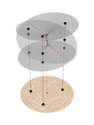
Figure 1: The homotopy graph (left) and the solution graph (right) viewed as a restriction of the 3-to-1 covering for $x^{3}+c=0$.

Assume that we know one solution (shaded in Figure 1) of $F_{p_{1}}$. Now continue this solution along edges of the solution graph. By doing so, we recover all three solutions at one of the nodes. As long as the action of the monodromy group (see [5] for definition and discussion) is transitive, it is always possible to recover all solutions from one by following along the edges of a graph that is sufficiently large and sufficiently general.

In our very simple example there is always a unique choice for the next edge to track along; in general, this will not be so. The fact that only a subgraph of the solution graph is known at any point of the algorithm complicates the selection of the next (homotopy continuation) atomic task further. Hence, two parts of the MS approach are probabilistic: first, the homotopy graph is created at random; and second, the task selection procedure may either be random or designed to maximize the expectation of some potential function (see §4) under a fixed probabilistic model.

It has been shown in [5] that given a simple probabilistic model, the expected number of edges in the solution graph for MS to succeed is linear in the number of solutions. This bounds the number of continuation tasks to be carried out and—what seems to be the main reason for the practical success of MS—ties the overall complexity of the approach to the actual number of the solutions, and not to some bound that may be available a priori for a larger family of systems (e.g., bound of Bézout or Bernstein-Khovanskii-Kouchnirenko).

Note that the Monodromy Solver framework does not specify a stopping criterion. For the discussion of possible stopping criteria see §3.2.2 and §3.2.3 of [5].

3 Definitions

Let $G$ be a loopless multigraph with vertices $V=V(G)$ and edges $E=E(G)$. Each vertex corresponds to a system $F_{p}$ specialized at parameters $p$ and is associated with $d$ solutions—we refer to the vertex together with this satellite data as a node. Each edge $e\in E$ connecting nodes $v_{1}$ and $v_{2}$ induces a homotopy that establishes a bijective correspondence between the solutions of the polynomial systems $F_{p_{1}}$ and $F_{p_{2}}$. We assume the following:

Assumption 1.

Edges induce uniformly random correspondences.

In other words, we assume that all bijective correspondences that could be induced by an edge connecting the solutions of $F_{p_{1}}$ and $F_{p_{2}}$ are equally likely. This assumption allows us to simplify the probability calculations and postulate an effective task selection strategy described in §4 especially when tracking multiple paths in parallel. See discussion of randomization in §5.1 of [5].

In general, $e$ will refer to an edge and $\vec{e}$ will refer to a directed edge (a pair of $e$ and a specified direction). A pair $t=(s,\vec{e})$, where $s\in S(v)$ belongs to the solution set $S(v)$ of the polynomial system corresponding to $v=\operatorname{src}{(\vec{e})}$, represents a candidate for (one) homotopy path track, an atomic task that shall be performed by one thread in a parallel algorithm.

We fix the graph $G=(V,E)$ at the initialization stage. At a given state $x=(Q,C,A)$ of the algorithm we have the following.

• A collection $Q$ of sets indexed by $v\in V$, where each $Q_{v}$ is the subset of solutions at $v$ known at this state.

• A collection $C$ of sets indexed by $e\in E$. Each $C_{e}\subset Q_{v}\times Q_{w}$ — where $v$ and $w$ are the nodes $e$ connects — is a partial one-to-one correspondence between subsets of $Q_{v}$ and $Q_{w}$. We denote by $\pi_{v}$ and $\pi_{w}$ the projections from $Q_{v}\times Q_{w}$ to $Q_{v}$ and $Q_{w}$, respectively.

• A set $A=\{t_{1},\dots,t_{k}\}$ of atomic (homotopy path tracking) tasks currently being processed (using $k$ independent threads).

Given a state $x=(Q,C,A)$ we denote $Q(x):=Q$, $C(x):=C$, and $A(x):=A$. Note that in most states (in our basic framework, in all states but the initial state) one can determine $Q$ from $C$. We shall call a state $x$ idle if $A(x)=\emptyset$.

For an atomic task $t=(s,\vec{e})\in A$, $\operatorname{src}(t)$ and $\operatorname{dest}(t)$ will refer to the source and destination vertices of $\operatorname{edge}(t):=\vec{e}$.

Prior to running $t,$ it is unknown which solution at $\operatorname{dest}(t)$ will be found. We use the random variable $\operatorname{sol}_{t}$ to denote the outcome of running this task, conditioned on the current state. Likewise, $\operatorname{sol}_{A}$ will denote the random set of solutions known after running the tasks in $A$. Suppose we know (or can estimate) the solution count for a generic system; refer to this (integer) count as $d$, the degree of the problem. Assumption 1 implies that

$$\Pr(\operatorname{sol}_{t}\notin Q_{\operatorname{dest}(\vec{e})})=\frac{d-|Q_{\operatorname{dest}(\vec{e})}|}{d-|C_{e}|}$$ (4)

Define $\operatorname{\mathbf{E}}(x)$ to be the expected total number of known solutions at all vertices after running all tasks $t\in A$ to completion. That is, if $y$ is the state after the completion, i.e., $A(y)=\emptyset$, then

$$\operatorname{\mathbf{E}}(x)=\sum_{v\in V(G)}\operatorname{\mathbf{E}}_{v}(x),\text{ with }\operatorname{\mathbf{E}}_{v}(x):=\operatorname{\mathbb{E}}(|Q_{v}(y)|),$$

where the (new) number of known points $|Q_{v}(y)|$ is perceived as a random variable with expected value $\operatorname{\mathbb{E}}(|Q_{v}(y)|)$; state transition probabilities are induced by Assumption 1.

4 Task selection via potential

We intend to use either $\operatorname{\mathbf{E}}(Q,C,A\cup\{t\})$ to define a potential function driving our choice of the next task $t$ to append to $A$ once a thread becomes available. The basic update rule is given below:

$$\operatorname{\mathbf{E}}_{v}(Q,C,A\cup\{t\})=\operatorname{\mathbf{E}}_{v}(Q,C,A)+\Pr(\operatorname{sol}_{t}\notin\operatorname{sol}_{A}).$$ (5)

This follows by a simple conditioning argument:

$$\operatorname{\mathbf{E}}_{v}(Q,C,A\cup\{t\}) =\operatorname{\mathbf{E}}_{v}(Q,C,A\cup\{t\}\mid\operatorname{sol}_{t}\in\operatorname{sol}_{A})\Pr(\operatorname{sol}_{t}\in\operatorname{sol}_{A})$$

$$+\operatorname{\mathbf{E}}_{v}(Q,C,A\cup\{t\}\mid\operatorname{sol}_{t}\notin\operatorname{sol}_{A})\Pr(\operatorname{sol}_{t}\notin\operatorname{sol}_{A})$$

$$=\operatorname{\mathbf{E}}_{v}(Q,C,A)\Pr(\operatorname{sol}_{t}\in\operatorname{sol}_{A})$$

$$+\Big{(}1+\operatorname{\mathbf{E}}_{v}(Q,C,A)\Big{)}\Pr(\operatorname{sol}_{t}\notin\operatorname{sol}_{A})$$

$$=\operatorname{\mathbf{E}}_{v}(Q,C,A)+\Pr(\operatorname{sol}_{t}\notin\operatorname{sol}_{A})$$

4.1 Potential given no path failures

Since random homotopy paths stay away from the discriminant locus with probability $1$, it is natural to seek a “smart” task-selection strategy in the idealized setting when no failures in homotopy tracking occur. The following proposition shows that $\operatorname{\mathbf{E}}_{v}(Q,C,A)$ can be computed recursively.

Proposition 1.

Let $v$ be a vertex and $e$ an edge incident to $v$. If $t$ is a candidate path track with $\operatorname{dest}(t)=v$ and $\operatorname{edge}(t)=\vec{e}$, then

$$\begin{aligned} \operatorname{\mathbf{E}}_{v}(Q,C,A\cup\{t\})&=\operatorname{\mathbf{E}}_{v}(Q,C,A)\\ &+\frac{d-\operatorname{\mathbf{E}}_{v}(Q,C,A)}{d-|C_{e}|-\#\{t^{\prime}\in A:\operatorname{edge}(t^{\prime})=\vec{e}\}}\end{aligned}$$ (6)

Thus, if we keep track of these expectations as we go, we may determine the potential of tracking a new thread without recomputing anything else.

Proof.

Let $X$ denote the random variable that, conditioned on the idle state $(Q,C,\emptyset),$ counts the total number of solutions at $v$ after completing all tasks in $A.$ Noting equation (5), we have

$$\Pr(\operatorname{sol}_{t}\notin\operatorname{sol}_{A})=$$

$$=\sum_{k\in\operatorname{supp}X}\displaystyle\frac{(d-k)}{d-|C_{e}|-\#\{t^{\prime}\in A:\operatorname{edge}(t^{\prime})=\vec{e}\}}\Pr(X=k)$$

$$=\frac{d-\operatorname{\mathbf{E}}_{v}(Q,C,A)}{d-|C_{e}|-\#\{t^{\prime}\in A:\operatorname{edge}(t^{\prime})=\vec{e}\}}.$$

∎

4.2 Potential in the presence of failures

The failure of certain atomic tasks is an inevitable feature of any MS implementation: such failures may occur when paths verge too close to the locus of singular systems, and may be influenced by the aggressiveness of threshold settings in the underlying numerical software as well as various others factors. In anticipation of such failures, we consider the effects of failures in a simple probabilistic model generalizing the results of the previous section.

Assumption 2.

We now assume that the probability of success for every atomic task equals a global fixed constant $\alpha\in[0,1]$ and that formation of edge correspondences and all task failures are mutually independent events.

Let us emphasize a technical feature of this assumption—if we have $\operatorname{edge}(t)=\operatorname{edge}(t^{\prime})$ and $\operatorname{dest}(t)=\operatorname{src}(t^{\prime}),$ the tasks $t$ and $t^{\prime}$ still fail independently. This lack of symmetry should be accounted for in any given state of the algorithm. Thus, we extend our definition of a state $x=(Q,C,A,F)$ as follows:

• As before, $Q_{v}$ denotes the set of solutions known at $v\in V,$ each $C_{vw}\subset Q_{v}\times Q_{w}$ is a set of known, successful correspondences, and $A$ is the set of current tasks.

• Failures are indexed by directed edges. For each $\vec{e}$, the set $F_{\vec{e}}$ consists of known solutions $s\in Q_{\operatorname{src}(e)}$ such that the task $(s,\vec{e})$ has completed with a failure. For $\alpha=1,$ we have $F_{\vec{e}}$ empty for all $\vec{e}$ and hence abbreviate $x=(Q,C,A).$

Proposition 2.

With notation as in Proposition 1,

$$\operatorname{\mathbf{E}}_{v}(Q,C,A\cup\{t\},F)=\operatorname{\mathbf{E}}_{v}(Q,C,A,F)\,+\alpha\times$$

$$\frac{\Big{(}d-\operatorname{\mathbf{E}}_{v}(Q,C,A,F)\Big{)}\Big{(}1-\operatorname{\mathbb{E}}\,\frac{\#F_{\operatorname{edge}(t)}+B}{d-\#C_{e}-\cdot\#\{t^{\prime}\in A\mid\operatorname{edge}(t^{\prime})=\vec{e}\}+B}\Big{)}}{d-\#C_{e}-\#F_{\operatorname{edge}(t)}-\#\{t^{\prime}\in A\mid\operatorname{edge}(t^{\prime})=\vec{e}\}}.$$

where $B$ a random variable with a binomial distribution: $B\sim\operatorname{Bin}(\#\{t^{\prime}\in A:\operatorname{edge}(t^{\prime})=\vec{e}\},1-\alpha).$

Proof.

Let $u=\operatorname{src}(\operatorname{edge}(t)).$ We consider the following set-valued random variables whose state spaces are conditional on the idle state $(Q,C,\emptyset,F):$

• $X$ is the set of all solutions at $v$ which are known after completing all tasks in $A$–hence $\operatorname{\mathbb{E}}[X]=\operatorname{\mathbf{E}}_{v}(Q,C,A).$

• $Y$ consists of all solutions at $v$ whose correspondences along $\vec{uv}$ have failed after completing all tasks in $A.$ Thus, the random variable $B:=(\#Y-\#F_{\operatorname{edge}(t)})$ has the desired binomial distribution.

Recalling (5), note that task $t$ yields a solution undiscovered by $A$ with probability $\alpha\cdot\Pr(\operatorname{sol}_{t}\notin\operatorname{sol}_{A}).$ Moreover, we have

$$\Pr(\operatorname{sol}_{t}\notin\operatorname{sol}_{A})=\displaystyle\frac{d-\operatorname{\mathbf{E}}_{v}(Q,C,A,F)-\operatorname{\mathbb{E}}[\#(Y\cap X^{c})]}{d-\#C_{e}-\#F_{\operatorname{edge}(t)}-\#\{t^{\prime}\in A\mid\operatorname{edge}(t^{\prime})=\vec{e}\}}$$

Conditional on the event $(X=k,B=j),$ we have that

$$\#Y=\#F_{\operatorname{edge}(t)}+j,$$

but the intersection $Y\cap X^{c}$ still depends on

$$d-(\#C_{e}+\#\{t^{\prime}\in A\mid\operatorname{edge}(t^{\prime})=\vec{e}\}-j)$$

unknown correspondences. Assumption 1 implies that the conditional distribution may be generated as follows:

• For each solution at $u$ which is known to fail along $\vec{uv}$ after completing all tasks in $A,$ the corresponding solutions in $Y$ are drawn uniformly without replacement from the $(d-\#C_{e}-\#\{t^{\prime}\in A\mid\operatorname{edge}(t^{\prime})=\vec{e}\}+j)$ solutions at $v$ without correspondences.

• Declare each solution in $Y\cap X^{c}$ to be a “success.”

Hence the conditional expectation of the number of “successes” is given by the mean of a hypergeometric distribution:

$$\operatorname{\mathbb{E}}\left(\#(Y\cap X^{c})\mid X=k,B=j\right)=$$ (7)

$$\displaystyle\frac{(\#F_{\operatorname{edge}(t)}+j)\,(d-k)}{d-\#C_{e}-\#\{t^{\prime}\in A\mid\operatorname{edge}(t^{\prime})=\vec{e}\}+j}$$ (8)

Averaging over $k$ and then $j$ gives the result. ∎

In practice, it is also useful to group current tasks together according to their directed edges. This is reflected in the following proposition:

Proposition 3.

Let $A\cup A^{\prime}$ denote the set of tasks, where $A^{\prime}$ consists of all tasks using the directed edge $\vec{uv}.$ Then

$$\operatorname{\mathbb{E}}_{v}(Q,C,A\cup A^{\prime},F)=\operatorname{\mathbb{E}}_{v}(Q,C,A,F)+\alpha\,\#A^{\prime}\,\left(\displaystyle\frac{d-\operatorname{\mathbb{E}}_{v}(Q,C,A,F)}{d-\#C_{e}}\right).$$

Proof.

Let $A^{\prime}=\{t_{1},\ldots,t_{k}\}$ and consider the events

$$E_{i}=\text{ ``}t_{i}\text{ finds a solution unknown after completing all tasks in }A\text{.''}$$

Then

$$\operatorname{\mathbb{E}}_{v}(Q,C,A\cup A^{\prime},F) =\operatorname{\mathbb{E}}_{v}(Q,C,A,F)+\displaystyle\sum_{i=1}^{k}\Pr(E_{i})$$

$$=\operatorname{\mathbb{E}}_{v}(Q,C,A,F)+\alpha\,\#A^{\prime}\,\Pr(\operatorname{sol}_{t_{1}}\notin\operatorname{sol}_{A})$$

$$=\operatorname{\mathbb{E}}_{v}(Q,C,A,F)+\alpha\,\#A^{\prime}\,\times$$

$$\displaystyle\frac{d-\operatorname{\mathbb{E}}_{v}(Q,C,A,F)-\Big{(}\frac{\#F_{\operatorname{edge}(t)}\cdot(d-\operatorname{\mathbb{E}}_{v}(Q,C,A,F))}{d-\#C_{e}}\Big{)}}{d-\#C_{e}-\#F_{\operatorname{edge}(t)}}$$

$$=\operatorname{\mathbb{E}}_{v}(Q,C,A,F)+\alpha\,\#A^{\prime}\,\times$$

$$\left(\displaystyle\frac{d-\operatorname{\mathbb{E}}_{v}(Q,C,A,F)}{d-\#C_{e}}\right).$$

∎

5 Algorithm

For every edge $\vec{e}$ we have its potential $\operatorname{\Delta}_{\vec{e}}(x)$ at state $x=(Q,C,A,F)$. The potential guides edge selection in our main algorithm below. Following the study in §4, the natural greedy potential aiming to maximize the expected total number of discovered solutions is

$$\operatorname{\Delta}_{\vec{e}}^{\operatorname{\mathbf{E}}}(x)=\operatorname{\mathbf{E}}(Q,C,A\cup\{(s,\vec{e})\},F)-\operatorname{\mathbf{E}}(x).$$

Algorithm 1 (Main algorithm).

The following is executed on all available threads after initializing the state $x=(Q,C,A,F)$.

 

  while $\nexists Q_{v}$ such that $|Q_{v}|=d$ do

     Pick an edge $\vec{e}=(w,v)$ that maximizes $\operatorname{\Delta}_{\vec{e}}(x)$ and such that there is $s\in Q_{w}\setminus\pi_{w}C_{e}$.

     $t\leftarrow(s,\vec{e})$

     Update the state: $x\leftarrow(Q,C,A\cup\{t\},F)$.

     Update $\operatorname{\Delta}(x)$.

     Run homotopy continuation for task $t$.

     if the run fails then

        $F_{\operatorname{edge}(t)}\leftarrow F_{\operatorname{edge}(t)}\cup\{s\}$.

     else

        Update $Q_{v}$, $C_{e}$, and $\operatorname{\Delta}$. {Note that an update is needed only for $\operatorname{\Delta}_{\vec{e^{\prime}}}$ such that $\operatorname{dest}(\vec{e^{\prime}})=v$.}

     end if

  end while 

Here are other (heuristic) potential functions we considered: :

$$\operatorname{\Delta}_{\vec{e}}^{\text{ord}}(x) = 1/i,$$

$$\text{where }v_{i}=\operatorname{dest}{\vec{e}}\quad\text{(assuming $i\in\{1,\dots,N\}$)}$$

$$\operatorname{\Delta}_{\vec{e}}^{\omega}(x) = \sum_{v\in V}\omega(v)\,\left(\operatorname{\mathbf{E}}_{v}(Q,C,A\cup\{(s,\vec{e})\},F)-\operatorname{\mathbf{E}}_{v}(x)\right),$$

$$\text{where weight }\omega(v)\in[0,1].$$

Note $\operatorname{\Delta}^{\text{ord}}$ is designed to bias edge selection towards nodes in their order of appearance. This potential is likely to force the algorithm to complete the solution set of the first node.

The weighted potential $\operatorname{\Delta}^{\omega}$ depends on the design of the weight function. See §7.3 for a family of weight functions that seems to be useful in practice.

In the initial idle state, $\operatorname{\Delta}$ can be computed and stored and then updated during the computation. Propositions 1 and 2 allow for an efficient way to do that in both sequential and parallel setting, with or without an assumption of failures.

6 Failure rate and threshold

With assumptions 1 and 2, suppose we have a complete multigraph on $N$ nodes with $m$ edges connecting each pair of nodes, $d$ solutions at each node, and tracking success probability $\alpha$. To each homotopy graph, we associate a solution (multi)graph whose vertices are given by all of the solutions at each node and whose edges are the successful correspondences between solutions. One possible instance of this random solution graph is depicted in Figure 2.

Figure 2: Solution multigraph w/ $N=3,d=4,$ $m=2.$

Note that the graph in Figure 2 has only $10$ edges out of a possible $24.$ Nevertheless, our algorithm succeeds in completing the bottom node whenever we start from one of the $9$ black solutions, which form a large connected component. We see that connectivity of the solution graph is sufficient, but not necessary, for our algorithm to terminate.

In our random solution graph model, define $A:=A_{m,N,d}$ to be the event that the algorithm starting at a random node terminates with $d$ solutions. We are interested in the asymptotic behavior of $\Pr(A)$ as $d\to\infty,$ with reasonable assumptions on $m$ and $N.$ More precisely, we wish to describe an interval $[a_{m,N,d},b_{m,N,d}]$ containing a threshold for the event $A;$ this means that for $\alpha(m,N,d)=o(a_{m,N,d}),$ we have $\Pr(A_{m,N,d})\to 0,$ while $\Pr(A_{m,N,d})\to 1$ if $\alpha(m,N,D)=\omega(b_{m,N,d}).$

The characterization of thresholds for various properties is a well-studied problem in random graph theory, particularly in the context of the Erdös-Renyi graph model. Our random solution graph does not enjoy the same asymptotic properties as the Edös-Renyi graph—since no two solutions at the same node may be connected, the graph is sparse, even for $\alpha$ near $1.$ Minding these difficulties, we provide a simple threshold region for the event $A$ in Proposition 4—see subsection 7.2 for experimental verification and further discussion.

Proposition 4.

With $m,N$ possibly depending on $d,$ we have the following large-$d$ asymptotics:

• If $\alpha(d)=o\left((Nm)^{-1}\right)$ and $N(d)=o\Big{(}\exp(d)\Big{)},$ then
  $\lim_{d\to\infty}\Pr(A_{m,N,d})=0.$

• If $\alpha(d)=\omega\left(\log d/m\right)$ and $N(d)=O(\log d),$ then
  $\lim_{d\to\infty}\Pr(A_{m,N,d})=1.$

We require a simple fact known as the Harris/Kleitman inequality, specialized to our model (cf. [1] pp. 86-87,  [2] pp. 39-41):

Theorem 1 (Harris/Kleitman Inequality).

If $\mathcal{A}$ and $\mathcal{B}$ are events in the random solution graph model which are upward-closed with respect to inclusion,

$$\Pr(\mathcal{A}\cap\mathcal{B})\geq\Pr(\mathcal{A})\times\Pr(\mathcal{B}).$$

In random graph theory, a property which is upward-closed with respect to inclusion is called a monotone increasing property. For us, monotone increasing simply means that increasing $\alpha$ does not decrease $\Pr(\mathcal{A})$ or $\Pr(\mathcal{B}).$ It is a famous result that every monotone property in the Erdös-Renyi model has a sharp threshold—for a precise statement, see [3].

Proof of Proposition 4.

Consider the following auxiliary events:

• $S:=S_{m,N,d,\alpha}$ will denote the event that there exists some node with a successful correspondence at each solution

• $C:=C_{m,N,d,\alpha}$ will denote the event that the solution graph is connected

Clearly we have

$$\Pr(C)\leq\Pr(A)\leq\Pr(S)$$ (9)

For part i), we may assume WLOG that $\alpha(d)>0$ for $d$ sufficiently large. Now, simply note that

$$\Pr(S) =1-\Pr(\text{ all nodes fail })$$

$$\leq 1-\displaystyle\prod_{j=1}^{N}\Pr(\text{node }j\text{ fails})$$ (Theorem 1)

$$\leq 1-\Big{(}1-(\alpha Nm)^{d}\Big{)}^{N}.$$

For $N=O(1)$ as $d\to\infty,$ we have

$$(1-(\alpha Nm)^{d})^{N}=(1-o(1)^{d})^{N}\to 1\text{ as }d\to\infty.$$

For the regime $\omega(1)=N(d)=o(\exp(d)),$ we have

$$(1-(\alpha Nm)^{d})^{N}\sim\exp(-(\alpha N^{1+1/d}m)^{d}),$$

which is $\omega(1)$ for $\alpha(d)=o(N^{-(1+1/d)}\,m^{-1})=o((Nm)^{-1}).$ In either regime, we have $\Pr(S)\to 0$ as $d\to\infty.$

To bound $\Pr(A)$ from below, let $v_{1},\ldots,v_{n}$ be the nodes of the homotopy graph and $G_{i}$ denote the subgraph of the solution graph induced by the solutions at nodes $v_{1}$ through $v_{i}.$ By repeated application of Theorem 1, we have

$$\Pr(C_{N}) =\Pr(C_{N-1}\cap\textrm{ each sol at }v_{N}\textrm{ has a nbr in }G_{N-1})$$

$$\geq\Pr(C_{N-1})\times\Pr(\textrm{each sol at }v_{N}\textrm{ has a nbr in }G_{N-1})$$

$$\geq\displaystyle\prod_{i=1}^{N}\Pr(\textrm{ all solutions at }v_{i}\textrm{ have a nbr in }G_{i-1})$$

$$=\displaystyle\prod_{i=1}^{N}\Big{(}1-(1-\alpha)^{(N-i)e}\Big{)}^{d}$$

$$\geq\Big{(}1-\exp(-\alpha m)\Big{)}^{Nd}$$

Now, setting

$$\alpha(d)=\displaystyle\frac{\log(d)\times\bigg{(}1+\log_{d}\big{(}N+g(d)\big{)}\bigg{)}}{m},$$

with $g(d)$ any function such that $g(d)\to\infty$ as $d\to\infty,$ we have

$$\Pr(C)\geq(1-g(d)/(Nd))^{Nd}\sim\exp\big{(}-g(d)\big{)}\to 1.$$

∎

7 Experimental Results

Our simulator enables the study of two types of experiments:

• Experiments analyzing fake solution graph data generated according to Assumptions 1 and 2, and

• experiments based on real parametric systems, for which all data — actual solutions, actual correspondences for edges in the graph, actual timings for each homotopy path that may be tracked — is harvested before the experimentation begins.

The simulator (code available at https://github.com/sommars/parallel-monodromy) proceeds in two stages:

• The first stage takes either randomly generated data using Assumption 1, which does not require running homotopy continuation, or collects the data through tracking homotopy paths with existing software.

• The second uses the datafile produced by the first. If several threads are simulated then we assume that there is no communication overhead, which is a close approximation of reality. Indeed, the messages passed around are rather short: a longest one contains coordinates of a newly discovered solution. This cost can be ignored in comparison to the cost of a homotopy continuation task.

From observed runs of PHCpack [23] and NumericalAlgebraicGeometry [13], we chose to model the time taken by each fake path track on the negative binomial distribution with parameters $p=0.3,$ $n=10$. For clarity and consistency with the results of §6, all simulations have been run using the complete graph configuration described in [5].

7.1 Parallel Performance

To demonstrate the quality of a parallel algorithm, the typical metrics used are speedup and efficiency (for textbook references, see [12], [27]). For a number of processors $p$, speedup is defined to be

$$S(p)=\frac{\text{sequential execution time}}{\text{parallel execution time}}$$ (10)

while efficiency is defined as

$$E(p)=\frac{S(p)}{p}\times 100\%$$ (11)

Ideally one would obtain $S(p)=p$ and $E(p)=100\%$, which means that all processor resources are constantly in use and no extra work is performed, compared to running the program with a single processor.

We ran two experiments to observe the efficiency of our algorithm, one with simulated data as in (1) and one with observed data as in (2). Table 1 contains efficiency results for the simulated data experiment, while Table 2 has efficiency results for the cyclic-$n$ roots problem.

#Solutions	100	500	1000	5000	10000
1	100%	100%	100%	100%	100%
2	98.87%	98.36%	99.88%	98.61%	99.3%
4	96.71%	96.34%	98.28%	99.75%	100.45%
8	91.92%	95.04%	97.55%	98.7%	100.56%
16	84.65%	92.82%	98.68%	99.24%	99.82%
32	71.39%	87.12%	94.89%	97.8%	100.74%
64	55.04%	78.78%	89.45%	96.7%	99.07%
128	35.95%	65.82%	79.62%	93.68%	97.87%

Table 1: Efficiency for simulated polynomial systems with varied numbers of solutions.

$n$	5	6	7	8	9	10
1	100%	100%	100%	100%	100%	100%
2	110.48%	98.34%	104.3%	99.41%	99.44%	109.02%
4	107.7%	98.57%	110.79%	103.06%	99.81%	107.62%
8	101.53%	98.23%	108.02%	108.59%	101.02%	106.58%
16	94.88%	91.52%	103.53%	100.53%	101.79%	103.91%
32	76.23%	86.73%	97.72%	100.81%	101.92%	105.54%
64	54.59%	70.47%	93.45%	98.62%	99.92%	102.88%
128	34.38%	52.37%	84%	96.23%	97.81%	102%

Table 2: Efficiency for cyclic-$n$ polynomial systems.

The cyclic $n$-roots problem is a classic benchmark problem in polynomial system solving, commonly formulated as

$$\begin{cases}x_{0}+x_{1}+\cdots+x_{n-1}=0\\ i=2,3,\ldots,n-1:\displaystyle\sum_{j=0}^{n-1}\leavevmode\nobreak\ \prod_{k=j}^{j+i-1}x_{k\leavevmode\nobreak\ {\textrm{m}od}\leavevmode\nobreak\ n}=0\\ x_{0}x_{1}x_{2}\cdots x_{n-1}-1=0.\\ \end{cases}$$ (12)

Both Tables 1 and 2 show the same relationships: as the number of threads increases, efficiency slowly decreases, and as the size of the problem increases, efficiency improves. This shows that it is an effective algorithm for running large systems in parallel, though it is unfortunate that for huge numbers of threads that efficiency decreases.

One could be concerned that Algorithm 1 would be slow to start, because initially a single node has a single solution. For small homotopy graphs with large numbers of threads, some threads will by necessity be idle until there are sufficiently many tasks available. Define

$$\%\text{Idle}=\frac{\sum_{i=1}^{p}\text{Idle time}}{\text{Wall time}\times p}.$$ (13)

As the number of solutions increases, $\%\text{Idle}$ approaches zero. It would be possible to make $\%\text{Idle}=0$ through a modification to Algorithm 1. When a thread rests idle waiting for a task to become available, it could define its own edge by picking a random $\gamma$ and tracking the sole known solution to a different node. In doing this, it has the potential to discover new solutions, but without adding to the known set of correspondences. Each thread could do this until it can be assigned a path track as the algorithm prescribes. However, this will provide only a minimal benefit, because the amount of idle time according to a wall clock is low.

7.2 Path Failures

The “probability-one” homotopy in a linear family $F_{p}$ fails with some nonzero probability. At fixed precision, this probability becomes non-negligible, say, as the degree of the discriminant rises. In practice, the reliability of homotopy continuation may be impacted by more aggressive path-tracking. For instance, raising the minimum step-size lowers the number of predictor steps, but there is a risk that errors accumulated may too large to finish continuation. In MS, this risk is spread across its incoming edges. Thus, we are interested in balancing tradeoffs between task reliability and speed.

Assumption 2 gives a simple model for path failures in a practical setting. An important feature of this model is that our simulator assumes a “true correspondence” between the solutions of two connected nodes before declaring that some of these paths fail. Thus, our model of failures ignores the phenomenon of path-jumping (potentially resulting in a 2-1 correspondence between approximate solutions,) or the possibility that some node has a near-singular solution. A logical next step would be to incorporate these possibilities into our model. However, we find that the simple model already sheds some light on the tradeoff previously described.

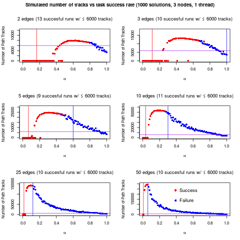
Figure 3: Total number of tracks vs task success rate $\alpha$ for varying edge multiplicities on a 3-node graph with 1000 solutions. The red and blue vertical lines given by $x=1/3m$ and $x=\log_{10}(d)/m,$ respectively, give an approximate window for the failure threshold. To give a sense of scale, a purple horizontal line at $y=6000$ has been added.

The plots in figure 3 supplement the results of Section 6. In each panel, the vertical distance equals the theoretical maximum number of tracks for each graph layout. Each run was performed with a single fake thread using the potential potE. These plots illustrate a major strength of using potentials in the presence of failures—even when additional edges are added, the number of path tracks at a fixed failure rate is stable (eg. at most 6000 for $\alpha\geq 0.9.$)

The bounds in Proposition 4 do not provide a useful upper bound on the threshold of global failure when the number of edges is relatively small (as in the top two plots of Figure 3.) We attempted to determine tighter threshold regions experimentally—see Table 3 for fabricated data and Table 4 for the cyclic $n$-roots problem.

$d\setminus N$	4	5	6	7	8	9
16	.716	.544	.426	.36	.332	.271
32	.756	.599	.495	.427	.362	.312
64	.771	.62	.537	.47	.391	.366
128	.799	.666	.584	.498	.453	.405
256	.841	.732	.634	.572	.497	.445
512	.873	.752	.674	.598	.536	.49

Table 3: An approximate threshold for the success rate $\alpha$. $N$ = the number of nodes in the complete graph (with $m=1$), $d$ = the number of solutions.

$n\setminus N$	5	6	7	8	9
5	.546	.492	.34	.298	.281
6	.605	.516	.416	.344	.316
7	.686	.611	.531	.452	.453
8	.734	.688	.647	.564	.492
9	.818	.733	.672	.629	.556

Table 4: An approximate threshold for the success rate $\alpha$ for the cyclic-$n$ family. $N$ = the number of nodes in the complete graph (with $m=1$).

7.3 Potential functions and edge selection

We defined potentials $\operatorname{\Delta}^{\operatorname{\mathbf{E}}}$, $\operatorname{\Delta}^{\text{ord}}$, and $\operatorname{\Delta}^{\omega}$. The last potential offers a lot of freedom to the user of the method. For instance, we could combine the ideas behind $\operatorname{\Delta}^{\operatorname{\mathbf{E}}}$ and $\operatorname{\Delta}^{\text{ord}}$ in $\operatorname{\Delta}^{\omega}$ by setting

$$\omega(v)=(|Q_{v}|/d)^{\lambda},\quad\lambda\geq 0,$$ (14)

where $d$ is the root count. (It could be replaced with the maximal number of solutions known at any node). Note that if $\lambda=0$, one gets $\operatorname{\Delta}^{\operatorname{\mathbf{E}}}$; for large $\lambda$ the effect is similar to that of $\operatorname{\Delta}^{\text{ord}}$ except the nodes are likely to be ordered according to the number of known solutions at any point of the execution.

In the sequential case, [5] shows that edge selection guided by the greedy potential $\operatorname{\Delta}^{\operatorname{\mathbf{E}}}$ outperforms several naive choices, among them the random edge selection strategy. According to our experiments this, as we expect, still holds for the parallel setting.

We conducted several experiments with the weight potential $\operatorname{\Delta}^{\omega}$ on graphs with edge multiplicity $m=1$ for fabricated and cyclic problems of degree up to $10000$ with and without failures. The weights described in (14) seem to deliver better (but not necessarily the best) performance as $\lambda\to\infty$. In other words, while a variant of the order potential $\operatorname{\Delta}^{\text{ord}}$ may serve as a good heuristic, there is still some room for improvement for edge selection strategies guiding the MS algorithm.

8 Conclusion

The benefits of the Monodromy Solver framework are demonstrated by an implementation in Macaulay2 [4, 6], which outperforms all existing blackbox polynomial system solvers on certain classes of problems. This is reported in §6.4 of the first article devoted to the framework [5].

The present work addressed items 1 (failures) and 3 (parallelization) in the program outlined in §7 of [5]. The experiments conducted with the simulator that we built, albeit not very extensive, shed light on the phenomena arising with the introduction of failures and parallel computation. The results of the experiments and the simulator itself will help to hone the core of the technique as well as construct efficient heuristics for software implementation in the future.

References

- [1] N. Alon and J. H Spencer. The probabilistic method. John Wiley & Sons, 2004.
- [2] B. Bollobás and O. Riordan. Percolation. Cambridge University Press, 2006.
- [3] B. Bollobás and A. G. Thomason. Threshold functions. Combinatorica, 7(1):35–38, Mar 1987.
- [4] T. Duff, C. Hill, A. Jensen, K. Lee, A. Leykin, and J. Sommars. MonodromySolver: a Macaulay2 package for solving polynomial systems via homotopy continuation and monodromy. Available at http://people.math.gatech.edu/aleykin3/MonodromySolver.
- [5] T. Duff, C. Hill, A. Jensen, K. Lee, A. Leykin, and J. Sommars. Solving polynomial systems via homotopy continuation and monodromy. To appear in IMA Journal of Numerical Analysis, 2018.
- [6] D. R. Grayson and M. E. Stillman. Macaulay2, a software system for research in algebraic geometry. Available at http://www.math.uiuc.edu/Macaulay2/.
- [7] T. Gunji, S. Kim, K. Fujisawa, and M. Kojima. Phompara – parallel implementation of the polyhedral homotopy continuation method for polynomial systems. Computing, 77(4):387–411, 2006.
- [8] S. Harimoto and L.T. Watson. The granularity of homotopy algorithms for polynomial systems of equations. In Proceedings of the Third SIAM Conference on Parallel Processing for Scientific Computing, pages 115–120, Philadelphia, PA, USA, 1989. Society for Industrial and Applied Mathematics.
- [9] J. Hauenstein, A. Sommese, and C. Wampler. Regeneration homotopies for solving systems of polynomials. Mathematics of Computation, 80(273):345–377, 2011.
- [10] J.D. Hauenstein, J.I. Rodriguez, and F. Sottile. Numerical computation of galois groups. arXiv preprint arXiv:1605.07806, 2016.
- [11] B. Huber and B. Sturmfels. A polyhedral method for solving sparse polynomial systems. Math. Comp., 64(212):1541–1555, 1995.
- [12] D.B. Kirk and W.W. Hwu. Programming Massively Parallel Processors: A Hands-on Approach. Morgan Kaufmann Publishers Inc., San Francisco, CA, USA, 1st edition, 2010.
- [13] A. Leykin. Numerical algebraic geometry. The Journal of Software for Algebra and Geometry, 3:5–10, 2011.
- [14] A. Leykin and F. Sottile. Computing monodromy via parallel homotopy continuation. In Proceedings of the 2007 International Workshop on Parallel Symbolic Computation, PASCO ’07, pages 97–98, New York, NY, USA, 2007. ACM.
- [15] A. Leykin and F. Sottile. Galois groups of Schubert problems via homotopy computation. Math. Comp., 78(267):1749–1765, 2009.
- [16] A. Leykin and J. Verschelde. Factoring solution sets of polynomial systems in parallel. In 2005 International Conference on Parallel Processing Workshops (ICPPW’05), pages 173–180, June 2005.
- [17] A. Leykin and J. Verschelde. Decomposing solution sets of polynomial systems: a new parallel monodromy breakup algorithm. International Journal of Computational Science and Engineering, 4(2):94–101, 2009.
- [18] A. Leykin, J. Verschelde, and Y. Zhuang. Parallel Homotopy Algorithms to Solve Polynomial Systems, pages 225–234. Springer Berlin Heidelberg, Berlin, Heidelberg, 2006.
- [19] A. Morgan. Solving polynomial systems using continuation for engineering and scientific problems. Prentice Hall Inc., Englewood Cliffs, NJ, 1987.
- [20] A.P. Morgan and L.T. Watson. A globally convergent parallel algorithm for zeros of polynomial systems. Nonlinear Analysis: Theory, Methods & Applications, 13(11):1339 – 1350, 1989.
- [21] A. J. Sommese, J. Verschelde, and C. W. Wampler. Using Monodromy to Decompose Solution Sets of Polynomial Systems into Irreducible Components, pages 297–315. Springer Netherlands, Dordrecht, 2001.
- [22] A.J. Sommese and C.W. Wampler. The numerical solution of systems of polynomials. World Scientific Publishing Co. Pte. Ltd., Hackensack, NJ, 2005.
- [23] J. Verschelde. Algorithm 795: PHCpack: A general-purpose solver for polynomial systems by homotopy continuation. ACM Trans. Math. Softw., 25(2):251–276, 1999. Available at http://www.math.uic.edu/jan.
- [24] J. Verschelde, P. Verlinden, and R. Cools. Homotopies exploiting newton polytopes for solving sparse polynomial systems. SIAM J. Numer. Anal., 31(3):915–930, June 1994.
- [25] J. Verschelde and Y. Zhuang. Parallel implementation of the polyhedral homotopy method. In 2006 International Conference on Parallel Processing Workshops (ICPPW’06), pages 8 pp.–488, 2006.
- [26] C.W. Wampler. Bezout number calculations for multi-homogeneous polynomial systems. Applied Mathematics and Computation, 51(2):143 – 157, 1992.
- [27] B. Wilkinson and M. Allen. Parallel Programming: Techniques and Applications Using Networked Workstations and Parallel Computers (2nd Edition). Prentice-Hall, Inc., Upper Saddle River, NJ, USA, 2004.