Noise-marginalized optimal statistic: A robust hybrid frequentist-Bayesian statistic for the stochastic gravitational-wave background in pulsar timing arrays

Abstract

Observations have revealed that nearly all galaxies contain supermassive black holes (SMBHs) at their centers. When galaxies merge, these SMBHs form SMBH binaries (SMBHBs) that emit low-frequency gravitational waves (GWs). The incoherent superposition of these sources produce a stochastic GW background (GWB) that can be observed by pulsar timing arrays (PTAs). The optimal statistic is a frequentist estimator of the amplitude of the GWB that specifically looks for the spatial correlations between pulsars induced by the GWB. In this paper, we introduce an improved method for computing the optimal statistic that marginalizes over the red noise in individual pulsars. We use simulations to demonstrate that this method more accurately determines the strength of the GWB, and we use the noise-marginalized optimal statistic to compare the significance of monopole, dipole, and Hellings-Downs (HD) spatial correlations and perform sky scrambles.

I Introduction

Long-wavelength gravitational waves (GWs) with frequencies of $10^{-9}-10^{-7}\;\mathrm{Hz}$ can be observed with pulsar timing arrays (PTAs) composed of millisecond pulsars (MSPs) Hellings and Downs (1983); Foster and Backer (1990). The dominant astrophysical source in this frequency range is the isotropic stochastic gravitational wave background (GWB) made up of the incoherent superposition of GWs from inspiraling supermassive black hole binaries (SMBHBs) (Rajagopal and Romani, 1995; Jaffe and Backer, 2003; Wyithe and Loeb, 2003). By monitoring the periodic emission from these pulsars using radio telescopes, we can probe the dynamics of the spacetime through which the pulses travel. This is done by searching for correlations in the pulsar timing residuals, which measure the differences between the expected and observed pulse times of arrival (TOAs). Current upper limits on the stochastic background from PTAs are approaching theoretical predictions for the GWB (Shannon et al., 2013; Lentati et al., 2015; Arzoumanian et al., 2018a)

PTAs primarily use Bayesian data analysis to compare the inferred probabilities of various models for the residuals, including one where they contain the GWB (van Haasteren et al., 2009; Lentati et al., 2013). Bayesian inference is a powerful tool because it properly accounts for degeneracies between parameters and incorporates all sources of uncertainty into the analysis. However, running a full Bayesian analysis is computationally intensive, particularly when searching for evidence of Hellings-Downs (HD) spatial correlations – the “smoking gun” of the GWB.

The significance of the GWB can also be assessed using the optimal statistic, a frequentist estimator for the GWB amplitude (Anholm et al., 2009; Demorest et al., 2013; Chamberlin et al., 2015). Not only does it provide an independent detection procedure, complementing a more robust Bayesian analysis, but it requires significantly less time to compute. In particular, the optimal statistic produces results for a given spatial correlation function within seconds; a full Bayesian analysis including correlations has to run for many weeks on a supercomputing cluster.

However, when pulsars have significant red noise the optimal statistic gives biased results due to the strong covariance between the individual red noise parameters and the GWB amplitude. Many individual pulsars show evidence for red noise (Lam et al., 2017; Arzoumanian et al., 2018b), and uncertainty in the position of the Solar System barycenter (SSB) leads to a common red process in all pulsars (Arzoumanian et al., 2018a). Here we present a technique for improving the accuracy of the optimal statistic by including an additional step: marginalizing over the individual pulsars’ red noise parameters using the posterior distributions from a full Bayesian analysis of all the pulsars. This hybrid approach produces a more precise estimate of the GWB amplitude $A_{\mathrm{gw}}$ and its uncertainty, while requiring only a few minutes more than the more traditional method of computation. Furthermore, the same Bayesian analysis drawn upon by the noise marginalization can be used to compute the optimal statistic for any choice of spatial correlations simply by changing the overlap-reduction function (ORF). For example, clock errors lead to a common red signal with monopole spatial correlations (Hobbs et al., 2012), while uncertainty in the SSB produces dipole spatial correlations (Champion et al., 2010). This technique is used to perform the frequentist searches for common red signals with HD, monopole, and dipole spatial correlations in the NANOGrav 11-year data set (Arzoumanian et al., 2018a).

This paper is organized as follows. In Sec. II we lay out the procedure for computing the noise-marginalized optimal statistic. We use simulations to compare the noise-marginalized optimal statistic to the optimal statistic computed with fixed noise. In Sec. III we determine how well the noise-marginalized optimal statistic can differentiate between monopole, dipole, and HD spatial correlations. In Sec. IV we use the noise-marginalized optimal statistic to perform sky scrambles, which assess the significance of HD spatial correlations by scrambling the pulsars’ sky positions (Cornish and Sampson, 2016; Taylor et al., 2017). We summarize our results in Sec. V as well as discuss future applications of the noise-marginalized optimal statistic.

II Noise-marginalized optimal statistic

The optimal statistic is a frequentist estimator for the amplitude of an isotropic stochastic GWB, and can be derived by analytically maximizing the PTA likelihood function in the weak-signal regime (Anholm et al., 2009; Chamberlin et al., 2015). It is constructed from the timing residuals $\delta{\bf t}$, which can be written as

$$\delta{\bf t}=M{\bf{\epsilon}}+F{\bf{a}}+U{\bf{j}}+{\bf{n}}\,.$$ (1)

The term $M\epsilon$ describes the contributions to the residuals from perturbations to the timing model. The term $U{\bf{j}}$ describes noise that is correlated for observations made at the same time at different frequencies and uncorrelated over different observing epochs, while ${\bf{n}}$ describes uncorrelated white noise from TOA measurement uncertainties. The term $F{\bf{a}}$ describes red noise, including both red noise intrinsic to the pulsar and a common red noise signal common to all pulsars (such as a GW signal). We model the red noise as a Fourier series,

$$F{\bf{a}}=\sum_{j=1}^{N}\left[a_{j}\sin\left(\frac{2\pi jt}{T}\right)+b_{j}\cos\left(\frac{2\pi jt}{T}\right)\right]\,,$$ (2)

where $N$ is the number of Fourier modes used (typically $N=30$) and $T$ is the span of the observations.

The optimal statistic is constructed from the autocovariance and cross-covariance matrices $C_{a}$ and $S_{ab}$,

$$C_{a} = \left\langle\delta{\bf t}_{a}\delta{\bf t}_{a}^{T}\right\rangle\,,$$ (3)

$$S_{ab} = \left.\left\langle\delta{\bf t}_{a}\delta{\bf t}_{b}^{T}\right\rangle\right|_{a\neq b}\,,$$ (4)

where $\delta{\bf t}_{a}$ is a vector of the residuals of the $a$th pulsar in the PTA. For the GWB with power spectral density (PSD) $P_{\mathrm{gw}}(f)$ and overlap reduction function (ORF) $\Gamma_{ab}$, the cross-covariance matrices are

$$S_{ab}=F_{a}\,\phi_{ab}^{\mathrm{gw}}\,F_{b}^{T}\,,$$ (5)

where

$$\phi_{ab}^{\mathrm{gw}}=\Gamma_{ab}\,P_{\mathrm{gw}}(f)\,.$$ (6)

The ORF is the HD curve (Hellings and Downs, 1983),

$$\Gamma_{ab} = \frac{1}{2}\left[1-\frac{1}{2}\left(\frac{1-\cos\theta_{ab}}{2}\right)\right.$$ (7)

$$\left.+3\left(\frac{1-\cos\theta_{ab}}{2}\right)\ln\left(\frac{1-\cos\theta_{ab}}{2}\right)\right]\,,$$

where $\theta_{ab}$ is the angle between the pulsars. We model the PSD of the GWB as a power law:

$$P_{\mathrm{gw}}(f)=\frac{A_{\mathrm{gw}}^{2}}{12\pi^{2}}\left(\frac{f}{f_{\mathrm{yr}}}\right)^{-\gamma}\,,$$ (8)

where $\gamma=13/3$ assuming SMBHBs evolve solely due to GW emission and $f_{\mathrm{yr}}\equiv 1/(1\,\mathrm{yr})$. The optimal statistic $\hat{A}^{2}$ is given by

$$\hat{A}^{2}=\frac{\sum_{ab}\delta{\bf t}_{a}^{T}{C_{a}^{-1}\tilde{S}_{ab}C_{b}^{-1}\delta{\bf t}_{b}}}{\sum_{ab}\operatorname{tr}\left(C_{a}^{-1}\tilde{S}_{ab}C_{b}^{-1}\tilde{S}_{ba}\right)}\,,$$ (9)

where $\tilde{S}_{ab}$ is the amplitude-independent cross-correlation matrix,

$$A_{\mathrm{gw}}^{2}\tilde{S}_{ab}=S_{ab}\,.$$ (10)

This definition of the optimal statistic ensures that $\langle\hat{A}^{2}\rangle=A_{\mathrm{gw}}^{2}$. If $A_{\mathrm{gw}}=0$, the variance of the optimal statistic is

$$\sigma_{0}=\left[\sum_{ab}\operatorname{tr}\left(C_{a}^{-1}\tilde{S}_{ab}C_{b}^{-1}\tilde{S}_{ba}\right)\right]^{-1/2}\,.$$ (11)

For a measured value of $\hat{A}^{2}$, the significance of $\hat{A}^{2}\neq 0$ is given by the signal-to-noise ratio (SNR)

$$\rho=\frac{\sum_{ab}\delta{\bf t}_{a}^{T}{C_{a}^{-1}\tilde{S}_{ab}C_{b}^{-1}\delta{\bf t}_{b}}}{\left[\sum_{ab}\operatorname{tr}\left(C_{a}^{-1}\tilde{S}_{ab}C_{b}^{-1}\tilde{S}_{ba}\right)\right]^{1/2}}\,.$$ (12)

When constructing the residuals $\delta{\bf t}_{a}$, we typically fix the red noise parameters to the values that maximize the single-pulsar likelihood. However, this leads to a bias in the optimal statistic because the individual red noise and common red noise parameters are highly covariant, with the optimal statistic computed using fixed red noise parameters systematically lower than the true value of $A_{\mathrm{gw}}^{2}$. In this section, we compare three techniques for computing the optimal statistic. First, we fix the individual pulsars’ red noise parameters to the maximum-likelihood values from individual Bayesian pulsar noise analyses. Second, we fix the pulsars’ red noise parameters to the values that jointly maximize the likelihood for a Bayesian analysis of all of the pulsars in our PTA that searches over the pulsars’ red noise parameters and a common red process. For the noise-marginalized method, we draw values of the pulsars’ red noise parameters from the posteriors generated by the common Bayesian analysis.

We use these methods to compute the optimal statistic for simulated “NANOGrav-like” data sets consisting of 18 MSPs with observation times, sky positions, and noise properties matching the 18 longest-observed pulsars in the NANOGrav 11-year data set (Arzoumanian et al., 2018b). We include white noise for all pulsars, plus red noise parametrized as a power law,

$$P_{a}(f)=\frac{A_{\mathrm{red}}^{2}}{12\pi^{2}}\left(\frac{f}{f_{\mathrm{yr}}}\right)^{-\gamma}\,,$$ (13)

for those pulsars that show evidence of red noise (see Table 1 for more details). We use the PTA data analysis package PAL2 (Ellis and van Haasteren, 2017) to perform the noise analyses and compute the optimal statistic.

Table 1: Pulsar parameters used in simulated PTA data sets.

Pulsar	$T_{\mathrm{obs}}$ (yrs)	$\sigma_{w}$ ($\mu\mathrm{s}$)	$A_{\mathrm{red}}$	$\gamma_{\mathrm{red}}$
J0030+0451	11.0	0.339	-13.93	3.56
J0613$-$0200	11.0	0.281	-13.14	1.22
J1012+5307	11.0	0.320	-12.79	1.51
J1024$-$0719	6.0	0.421	$-$	$-$
J1455$-$3330	11.0	0.773	$-$	$-$
J1600$-$3053	8.0	0.146	$-$	$-$
J1614$-$2230	7.0	0.261	$-$	$-$
J1640+2224	11.0	0.202	$-$	$-$
J1713+0747	11.0	0.093	-14.14	1.58
J1741+1351	6.0	0.106	$-$	$-$
J1744$-$1134	11.0	0.096	$-$	$-$
B1855+09	11.0	0.218	-13.75	3.54
J1853+1303	7.0	0.215	$-$	$-$
J1909$-$3744	11.0	0.034	-13.84	1.74
J1918$-$0642	11.0	0.342	$-$	$-$
J2010$-$1323	7.0	0.413	$-$	$-$
J2145$-$0750	11.0	0.281	-12.69	1.30
J2317+1439	11.0	0.160	$-$	$-$

Figure 1 shows the fixed-noise and noise-marginalized optimal statistic for a simulation with a GWB with $A_{\mathrm{gw}}=5\times 10^{-15}$. For this particular realization of the GWB, the fixed-noise analysis using the individual noise results gives $\hat{A}^{2}=6.6\times 10^{-30}$ with $\mathrm{SNR}=2.4$, and the fixed-noise analysis using the common noise results gives $\hat{A}^{2}=2.1\times 10^{-29}$ with $\mathrm{SNR}=4.7$. The noise-marginalized analysis gives $\hat{A}^{2}=(2.5\pm 0.1)\times 10^{-29}$ with $\mathrm{SNR}=4.8\pm 0.8$. The value of $\hat{A}^{2}$ from the fixed-noise analysis using the individual noise results is significantly lower than the injected level of the GWB, while the values of $\hat{A}^{2}$ from the fixed-noise analysis using the common noise results and the noise-marginalized analysis are in good agreement with each other and the injected value. The fixed-noise analysis using the individual noise results also gives a significantly lower SNR than the other two.

In Fig. 2 we show the optimal statistic for 300 different realizations of a GWB with $A_{\mathrm{gw}}=5\times 10^{-15}$ computed using the three techniques described above. For the noise-marginalized analysis, we plot the mean values of $\hat{A}^{2}$ and $\rho$. Using the noise values from individual noise analyses systematically underestimates the strength of the GWB, while using the noise values from a common noise analysis more accurately recovers the injected value. The fixed-noise analysis using the individual noise results finds $\hat{A}^{2}=(7.9\pm 6.8)\times 10^{-30}$ and $\rho=2.3\pm 1.5$, averaging over realizations of the GWB. The fixed-noise and noise-marginalized analyses using the common noise results both give $\hat{A}^{2}=(2.4\pm 1.2)\times 10^{-29}$ and $\rho=4.1\pm 1.7$.

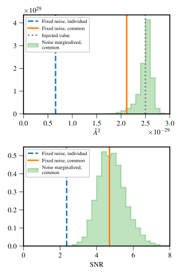
Figure 1: Optimal statistic for a simulated PTA data set containing a GWB with $A_{\mathrm{gw}}=5\times 10^{-15}$. The fixed-noise analysis using the individual noise values (dashed blue lines) systematically underestimates $\hat{A}^{2}$, while the fixed-noise analysis using the common noise values (solid orange lines) and the noise-marginalized analysis (green histograms) more accurately recover $A_{\mathrm{gw}}$.

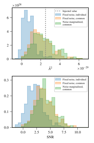
Figure 2: Optimal statistic and SNR for 300 simulated data sets containing a GWB with $A_{\mathrm{gw}}=5\times 10^{-15}$. The fixed-noise analysis using the individual noise values (blue) systematically underestimates $\hat{A}^{2}$, while both the fixed-noise analysis using the common noise values (orange) and the noise-marginalized analysis (green) accurately recover $A_{\mathrm{gw}}$.

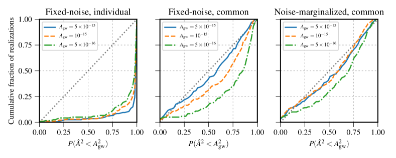
Figure 3: P–P plot showing the cumulative fraction of simulations for which $A_{\mathrm{gw}}^{2}$ lies within a given confidence interval of the measured $\hat{A}^{2}$. The probability distribution of $\hat{A}^{2}$ is assumed to be a Gaussian with variance $\sigma^{2}_{\hat{A}^{2}}$. The fixed-noise optimal statistic using the individual and common noise results both give biased values of $\hat{A}^{2}$, particularly for small values of $A_{\mathrm{gw}}$, while the noise-marginalized optimal statistic gives more accurate values of $\hat{A}^{2}$ over a large range of injected values of $A_{\mathrm{gw}}$.

The fixed-noise and noise-marginalized analyses using the common noise results give the same results for $A_{\mathrm{gw}}=5\times 10^{-15}$, but there are differences between them when analyzing data sets containing smaller injected values of $A_{\mathrm{gw}}$. In Fig. 3 we show a P–P plot of the cumulative fraction of simulations for which the injected $A_{\mathrm{gw}}^{2}$ lies within a given confidence interval of the measured $\hat{A}^{2}$. The confidence interval of $\hat{A}^{2}$ is determined assuming $\hat{A}^{2}$ follows a Gaussian distribution, with mean and variance $\sigma^{2}_{\hat{A}^{2}}$ taken from the distribution for $\hat{A}^{2}$ found from our 300 realizations of the GWB (i.e., the top panel of Fig. 2). If $\hat{A}^{2}$ has a Gaussian distribution centered around $A_{\mathrm{gw}}^{2}$, the curves should lie along a straight line with slope equal to unity (the dotted, diagonal lines in Fig. 3).

We compare the three methods for computing the optimal statistic for simulations with $A_{\mathrm{gw}}=5\times 10^{-15}$, $A_{\mathrm{gw}}=10^{-15}$, and $A_{\mathrm{gw}}=5\times 10^{-16}$. The fixed-noise optimal statistic using the individual noise results systematically underestimates $\hat{A}^{2}$ (Fig. 3, left panel). The fixed-noise optimal statistic using the common noise results recovers $\hat{A}^{2}$ well for large values of $A_{\mathrm{gw}}$, but for small values it also underestimates $\hat{A}^{2}$ (Fig. 3, middle panel). The noise-marginalized optimal statistic provides the most accurate estimate of $\hat{A}^{2}$ over the range of $A_{\mathrm{gw}}$ considered here, although it still slightly underestimates $A_{\mathrm{gw}}$ (Fig. 3, right panel).

III Monopole and Dipole Spatial Correlations

The optimal statistic is particularly well-suited to compare multiple spatial correlation relations because using a different spatial correlation only requires changing the ORF in Eq. (6). Tiburzi et al. (2016) demonstrated how the optimal statistic can be altered to fit for multiple spatial correlations at once in order to mitigate common noise sources such as clock error and ephemeris error. Here we take a different approach – rather than simultaneously fitting for signals with different spatial correlations, we look at how well we can distinguish between different spatial correlations by computing the optimal statistic with monopole and dipole spatial correlations for the same simulated data sets as in the previous section. For a monopole signal, the ORF becomes simply $\Gamma_{ab}=1$, while for a dipole signal, the ORF becomes $\Gamma_{ab}=\cos\theta_{ab}$.

Our ability to distinguish between different spatial correlations depends on the strength of the GWB and the angular separations between pulsar pairs, $\theta_{ab}$. We can determine the overlap between ORFs corresponding to different spatial correlations by computing the “match statistic” (Cornish and Sampson, 2016),

$$\bar{M}=\frac{\sum_{a,b\neq a}\Gamma_{ab}\Gamma^{\prime}_{ab}}{\sqrt{\left(\sum_{a,b\neq a}\Gamma_{ab}\Gamma_{ab}\right)\left(\sum_{a,b\neq a}\Gamma^{\prime}_{ab}\Gamma^{\prime}_{ab}\right)}}\,,$$ (14)

where $\Gamma$ and $\Gamma^{\prime}$ are two different ORFs. For the 18 pulsars used in these simulations, the match statistic for monopole and HD correlations is $\bar{M}=0.264$, and the match statistic for dipole and HD correlations is $\bar{M}=0.337$. These match statistics describe a fundamental limit on our ability to identify the spatial correlations of a common red signal as HD rather than monopole or dipole that depends only on the number of pulsars in our PTA and their sky positions.

Figure 4 shows the noise-marginalized mean value of $\hat{A}^{2}$ and the mean SNR computed assuming monopole, dipole, and HD spatial correlations for 300 simulated data sets. Using a monopole or dipole ORF gives a lower value for the mean optimal statistic and mean SNR compared to the HD ORF. Using HD spatial correlations gives $\hat{A}^{2}=(2.4\pm 1.1)\times 10^{-29}$, while using monopole spatial correlations gives $\hat{A}^{2}=(2.5\pm 3.2)\times 10^{-30}$, and dipole spatial correlations gives $\hat{A}^{2}=(5.2\pm 4.4)\times 10^{-30}$. We find a noise-marginalized mean SNR above 1.0 in 97% of our simulated data sets using the HD ORF, and in 50% and 68% of our simulated data sets using the monopole and dipole ORFs, respectively. The mean SNR using the HD ORF, averaged over realizations of the GWB, is 4.1, and we find an SNR greater than this using the monopole and dipole ORFs in just 3% and 3.5% of our simulations, respectively.

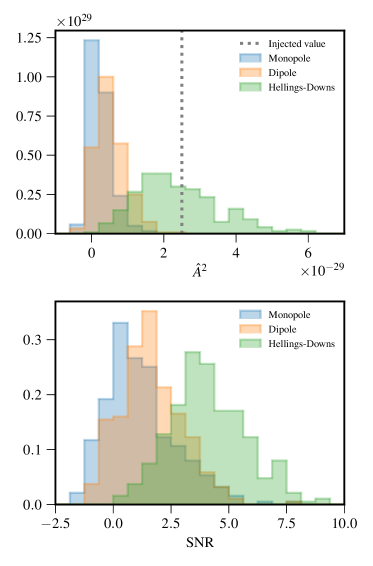
Figure 4: Noise-marginalized mean optimal statistic and mean SNR for 300 simulated data sets containing an injected GWB with $A_{\mathrm{gw}}=5\times 10^{-15}$. We compare the values of the mean optimal statistic and the SNR found using monopole (blue), dipole (orange), and HD (green) spatial correlations. The dashed vertical line indicates the injected value, $\hat{A}^{2}=2.5\times 10^{-29}$.

This overlap between the monopole, dipole, and HD ORFs also means that a common red process that does not have HD correlations may be confused for a GWB. Figure 5 shows the results of 300 simulations containing a stochastic signal with dipole spatial correlations. Although a dipole signal has been injected, the HD ORF gives a mean SNR greater than 5 in 82% of the simulations. However, both the monopole and HD ORFs give smaller values of the mean $\hat{A}^{2}$ and mean SNR compared to the dipole ORF. Furthermore, there are no simulations for which the mean SNR with HD ORF is greater than the mean SNR with dipole ORF. This demonstrates the importance of comparing the SNR from different spatial correlations when determining the type of spatial correlations present.

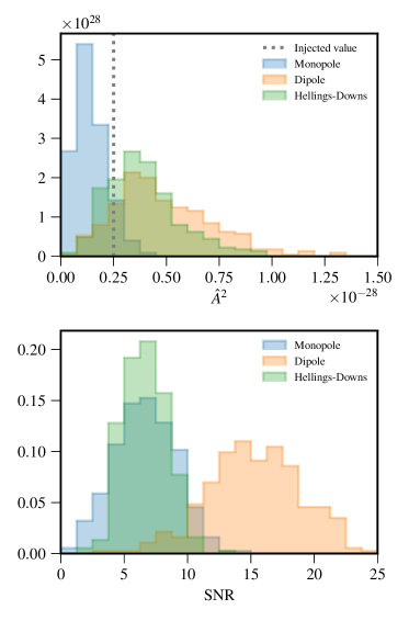
Figure 5: Noise-marginalized mean optimal statistic and mean SNR for 300 simulated data sets containing an injected stochastic signal with dipole spatial correlations and $A=5\times 10^{-15}$. We compare the values of the optimal statistic and mean SNR found using monopole (blue), dipole (orange), and HD (green) spatial correlations. The dashed vertical line indicates the injected value, $\hat{A}^{2}=2.5\times 10^{-29}$.

IV Sky Scrambles

The significance of spatial correlations can also be tested with “sky scrambles,” where the ORF is altered in order to simulate changing the pulsars’ positions (Cornish and Sampson, 2016; Taylor et al., 2017). The scrambled ORFs are required to have small values of $\bar{M}$ with the true ORF and each other so that they form a nearly orthogonal set. This ensures that the distribution of $\hat{A}^{2}$ computed using the scrambled ORFs forms the null hypothesis distribution. Taylor et al. (2017) showed how sky scrambles affect the Bayes’ factor for simulated data sets. We performed a similar analysis using frequentist methods.

We generated 725 scrambled ORFs using a Monte Carlo algorithm. We required the scrambled ORFs to have $\bar{M}<0.2$ with respect to the true ORF and each other. This threshold was chosen to be comparable to the match statistics between the HD ORF with monopole and dipole ORFs given in Sec. III. We did not choose a smaller threshold because significantly more time would have been needed to generate 725 scrambled ORFs. For each simulation, we computed the noise-marginalized mean optimal statistic and mean SNR for each scrambled ORF, and compared them to the values found using the true ORF.

Figure 6 shows the results of a sky scramble analysis for a sample data set with $A_{\mathrm{gw}}=5\times 10^{-15}$. For this particular realization of the GWB, none of the 725 scrambled ORFs resulted in a mean SNR greater than the mean SNR using the true ORF ($p<0.0014$). In Fig. 7, we plot the distribution of $p$-values of the 725 sky scrambles for 300 realizations of the GWB. For a GWB with $A_{\mathrm{gw}}=5\times 10^{-15}$, 95% of the simulations have $p\leq 0.05$, and 74% of the simulations have $p\leq 0.003$. For a GWB with $A_{\mathrm{gw}}=10^{-15}$, 76% of the simulations have $p\leq 0.05$, and 39% have $p\leq 0.003$. This shows that for smaller values of $A_{\mathrm{gw}}$, there is a greater chance that noise fluctuations will appear to have the spatial correlations of the GWB.

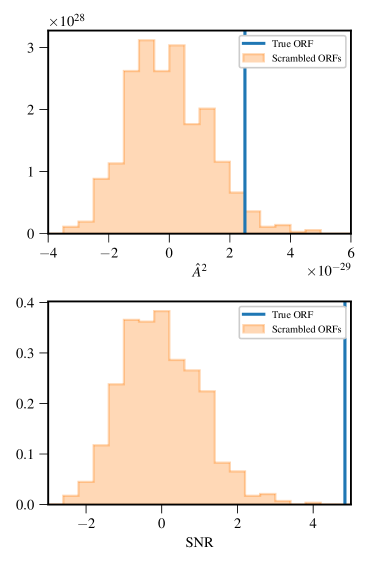
Figure 6: Comparison between the noise-marginalized mean optimal statistic and mean SNR with and without sky scrambles for a simulated data set containing a GWB with $A_{\mathrm{gw}}=5\times 10^{-15}$. None of the 725 scrambled ORFs gave a mean SNR as large as the mean SNR using the true ORF ($p<0.0014$).

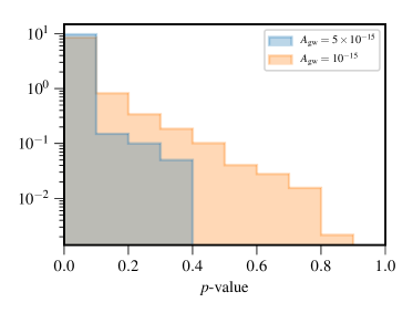
Figure 7: Distribution of $p$-values for the noise-marginalized optimal statistic mean SNR using the true ORF compared to 725 sky scrambles from 300 realizations of the GWB. We show results for simulations with $A_{\mathrm{gw}}=5\times 10^{-15}$ (blue) and $A_{\mathrm{gw}}=10^{-15}$ (orange).

V Conclusion

The definitive signature of a GWB in PTA data is spatial correlations described by the HD curve. Searching for these using a full Bayesian approach is computationally expensive, requiring many weeks on a supercomputing cluster. In contrast, the optimal statistic can be computed in seconds. In this paper, we introduce an improved method for computing the optimal statistic, which uses the output from a Bayesian analysis for individual and common red signals to marginalize the optimal statistic over the individual pulsars’ red noises. As shown in Sec. II, the noise-marginalized optimal statistic more accurately recovers the GWB amplitude than the fixed-noise optimal statistic, which underestimates the GWB amplitude when significant red noise is present in some pulsars.

Although the noise-marginalized optimal statistic requires computing the optimal statistic thousands of times, it is still many orders of magnitude faster than a Bayesian search. Furthermore, the results from a single Bayesian analysis, which are needed to marginalize over the red noise parameters, can be used to compute the optimal statistic for many different spatial correlations. In Sec. III we use the noise-marginalized optimal statistic to compare the strength of monopole, dipole, and HD correlations in simulated PTA data with a GWB. In Sec. IV we use the noise-marginalized optimal statistic to perform sky scramble analyses, where we compare the mean SNR computed using the true ORF to the mean SNR computed using scrambled ORFs and measure the significance of HD spatial correlations through the $p$-value.

The primary strength of the optimal statistic is how quickly it can be computed. This is useful for analyses where the significances of many spatial correlations are compared, as with the sky scrambles. An upcoming paper will use the noise-marginalized optimal statistic to determine how well the spatial correlations corresponding to alternate GW polarizations can be measured. It also makes the optimal statistic a valuable tool for analyzing simulations where many realizations of the GWB are compared. The noise marginalization technique described in this paper is key to being able to accurately measure the GWB with the optimal statistic for real PTAs and realistic PTA simulations, for which red noise is significant.