Low-frequency Alfvén Waves Produced by Magnetic Reconnection in the Sun’s Magnetic Carpet

Abstract

The solar corona is a hot, dynamic, and highly magnetized plasma environment whose source of energy is not yet well understood. One leading contender for that energy source is the dissipation of magnetohydrodynamic (MHD) waves or turbulent fluctuations. Many wave-heating models for the corona and the solar wind presume that these fluctuations originate at or below the Sun’s photosphere. However, this paper investigates the idea that magnetic reconnection may generate an additional source of MHD waves over a gradual range of heights in the low corona. A time-dependent Monte Carlo simulation of the mixed-polarity magnetic field is used to predict the properties of reconnection-driven coronal MHD waves. The total power in these waves is typically small in comparison to that of photosphere-driven waves, but their frequencies are much lower. Reconnection-driven waves begin to dominate the total power spectrum at periods longer than about 30 minutes. Thus, they may need to be taken into account in order to understand the low-frequency power-law spectra observed by both coronal spectropolarimetry and in situ particle/field instruments. These low-frequency Alfvén waves should carry more magnetic energy than kinetic energy, and thus they may produce less nonthermal Doppler broadening (in comparison to photosphere-driven high-frequency waves) in emission lines observed above the solar limb.

The Astrophysical Journal, 2018, in press

1 Introduction

The physical processes responsible for heating the solar corona and accelerating the solar wind have not yet been identified definitively. Some theoretical proposals involve magnetohydrodynamic (MHD) waves that originate at or below the solar photosphere, propagate up into the corona, and dissipate their energy as heat (e.g., Alfvén, 1947; Osterbrock, 1961; Hollweg, 1986; Matthaeus et al., 1999; Suzuki & Inutsuka, 2006; Cranmer et al., 2007; Lionello et al., 2014). Other ideas focus on the energy released by magnetic reconnection events in the upper atmosphere (Gold, 1964; Parker, 1972, 1988; Heyvaerts & Priest, 1984; Parnell & De Moortel, 2012) that may break open field lines that were formerly closed (Fisk et al., 1999; Fisk, 2003, 2005; Antiochos et al., 2011; Edmondson, 2012). Both classes of models appear to predict heating that is highly intermittent in both space and time (e.g., van Ballegooijen et al., 2011; Klimchuk, 2015) as is observed in the corona (Fletcher et al., 2015). This fact—combined with the existence of a highly structured “magnetic carpet” of mixed-polarity fields at the coronal base (Title & Schrijver, 1998)—has led to the conjecture that a realistic description of coronal heating involves both waves and reconnection.

It should come as no surprise that oscillatory MHD fluctuations (i.e., waves, shocks, and turbulent eddies) and magnetic reconnection events coexist with one another and may be of comparable importance in the corona’s energy budget. In fact, it is increasingly difficult to find simulations that contain only turbulence with no reconnection, or only reconnection with no turbulence (see, e.g., Velli et al., 2015). The focus of this paper is on one aspect of this linkage: the spontaneous generation of MHD waves from discrete magnetic reconnection events in the corona. This general idea has been studied in the past from the standpoint of infrequent flux-cancellation events (Hollweg, 1990) or a persistent “furnace” of mixed-polarity activity in the supergranular network (Axford & McKenzie, 1992; Ruzmaikin & Berger, 1998). Increasingly sophisticated models of reconnection in both the chromosphere (Sturrock, 1999; Isobe et al., 2008) and the corona (Lynch et al., 2014; Thurgood et al., 2017; Karpen et al., 2017; Tarr, 2017) also show wavelike oscillations as a natural by-product.

Coronal jets and solar flares are notable and observable testbeds for understanding how reconnection produces waves. Jets are dense and collimated eruptions that appear to accelerate plasma into open-field regions connected to the solar wind (Raouafi et al., 2016). These relatively infrequent events often are seen to produce swaying motions of the magnetic field, indicative of transverse or toroidal MHD waves (Cirtain et al., 2007; Moore et al., 2011, 2015; Yang et al., 2015; Szente et al., 2017). Simulations also predict the generation of waves and turbulence from individual jets (Lee et al., 2015; Jelínek et al., 2015; Wyper et al., 2016; Uritsky et al., 2017). Solar flares are powered by intense bursts of magnetic reconnection, and they may generate downward-propagating MHD waves that are important to the subsequent radiative emission (Emslie & Sturrock, 1982; Fletcher & Hudson, 2008; Reep & Russell, 2016). Oscillatory behavior has also been seen above flare loop-tops (Takasao & Shibata, 2016), in flare ribbons (Brannon et al., 2015), and in post-flare arcades (Verwichte et al., 2005).

This paper represents an attempt to predict some broad properties (e.g., energy levels and power spectra) of the MHD fluctuations generated by the Sun’s magnetic carpet. Section 2 describes the Monte Carlo simulations that were used to model the relevant reconnection and loop-opening (RLO) processes. Section 3.1 outlines a method of extracting the fluxes and magnetic perturbation profiles of Alfvénic pulses associated with individual reconnection events in the simulation. Section 3.2 then presents simulated wave power spectra that were extracted from the simulations, and discusses time-averaged energy densities. Section 4 contains some speculation about how these waves are likely to propagate up through the corona in a manner that departs from the standard WKB (Wentzel, Kramers, Brillouin) theory. Lastly, Section 5 gives a brief summary of the major results and discusses some of the broader implications of this work.

2 The Monte Carlo Magnetic Carpet Model

Cranmer & van Ballegooijen (2010) developed a three-dimensional simulation of photospheric magnetic flux transport that was coupled with a potential-field coronal extrapolation. The main goal of this model was to determine the rates at which closed field lines open up (i.e., to find the recycling timescale for open flux) and to estimate how much magnetic energy is released in reconnection events that involve the opening up of closed loops. Figure 1 illustrates the closed and open field lines associated with a typical time snapshot of the model.

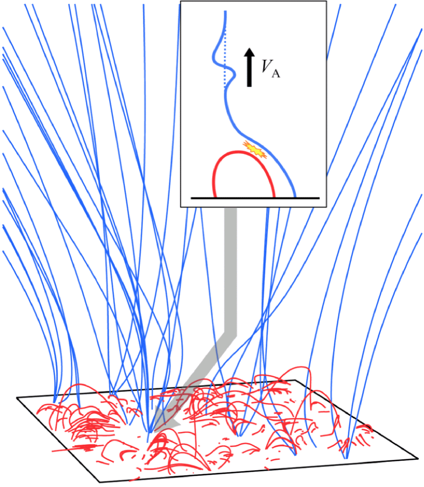
Figure 1: Open (blue) and closed (red) magnetic field lines traced in three-dimensional space for an example timestep in the Monte Carlo model with $\xi=0.5$ and absolute flux density $B_{\rm abs}=4$ Mx cm^-2. The horizontal box outlines the (200 Mm)² photospheric simulation domain at the base, and the maximum height of the closed field lines is 18 Mm. The inset shows a cartoon illustration of a single “interchange reconnection” event that produces an upward propagating wavelike perturbation along a newly opened field line.

The Cranmer & van Ballegooijen (2010) simulations comprise four successive stages:

1. The complex photospheric field is modeled by means of a Monte Carlo ensemble of positive and negative monopole sources of magnetic flux (see, e.g., Schrijver et al., 1997). The pointlike flux sources are assumed to emerge from below (in bipolar pairs), randomly diffuse across the surface, merge or cancel with their neighbors, and occasionally fragment into multiple pieces. The system is evolved with discrete timesteps $\Delta t$, and it approaches a state of dynamical equilibrium in which the net rate of magnetic cancellation balances the rate of emergence.

2. At each new timestep, the coronal magnetic field is recomputed from the current configuration of photospheric flux elements. Each element is assumed to act as a monopole-type source, and the summed vector extrapolation is a so-called potential field. Strictly speaking, this is a minimum-energy state that is unable to release “free energy” by undergoing magnetic reconnection. The relative shortcomings and advantages of this idealization were discussed in detail by Cranmer & van Ballegooijen (2010), but it is important to note that the potential-field assumption has been found to be useful in at least identifying the locations of the small regions in which coronal reconnection must occur (Close et al., 2003, 2005; Régnier et al., 2008).

3. Given a range of criteria that locate photospheric flux elements that “survive” from one timestep to the next, the Cranmer & van Ballegooijen (2010) code searches for events in which an initially closed field line at time $t$ changes into an open field line at $t+\Delta t$. These are assumed to be the sites of interchange reconnection. For each of these events, the code outputs the magnitude of magnetic flux $\Phi_{\rm co}$ connected to the footpoint that remains rooted to the surface, the horizontal distance $d$ to the other footpoint at time $t$, and the mean $x,y$ position of the footpoint (averaged over time steps $t$ and $t+\Delta t$).

4. Lastly, the amount of nonpotential energy release at each coronal reconnection event is estimated using a quasi-static minimum-current corona (MCC) theory (Longcope, 1996). This model depends on a time-averaged idealization of the amount of current that must build up—and subsequently dissipate—along a magnetic separator in the corona. It does not specify how the dissipated free energy is partitioned into other forms such as thermal energy, bulk kinetic energy, waves, and energetic particles. However, the MCC theory has been found to provide realistic predictions of the overall reconnection rate (see also Longcope, 2001; Longcope & Kankelborg, 1999; Beveridge & Longcope, 2006; Tarr & Longcope, 2012). In the present simulations, the total rate of energy loss (summed over the domain shown in Figure 1) is found to be appropriately bursty and nanoflare-like.

As a shorthand notation, the phrase “Monte Carlo model” will be used in this paper to describe the entire Cranmer & van Ballegooijen (2010) simulation, despite the fact that only the first of the above four stages depends on actual Monte Carlo randomization.

Cranmer & van Ballegooijen (2010) summarized the MCC method of estimating the power $P_{\rm co}$ released by each reconnection event, with

$$P_{\rm co}\,=\,\theta_{\rm L}C_{\rm L}\frac{\Phi_{\rm co}}{d}\left|\frac{d\Phi}{dt}\right|\,\,,$$ (1)

and $\theta_{\rm L}$ and $C_{\rm L}$ are dimensionless constants that describe the efficiency and magnetic separator geometry. It is assumed that the Monte Carlo time step $\Delta t$ characterizes the timescale over which individual reconnection events take place, so the time derivative above can be estimated as $|d\Phi/dt|\approx\Phi_{\rm co}/\Delta t$. Thus, the total free energy $E_{\rm co}$ released by each event is given by the power multiplied by $\Delta t$, and

$$E_{\rm co}\,\approx\,\theta_{\rm L}C_{\rm L}\frac{\Phi_{\rm co}^{2}}{d}\,\,.$$ (2)

This quantity is used below to estimate the maximum energy available to drive an Alfvén-wave packet associated with a given event. The value of the discrete timestep was chosen to be $\Delta t=5$ min. Larger values were found to sometimes skip over some potentially important energy-release events. Smaller values of $\Delta t$ ended up subdividing some reconnection events into smaller pieces, but with summed values of $E_{\rm co}$ being similar to the standard choice of 5 min. However, with such short timesteps (e.g., $\Delta t\lesssim 1$ min), the photospheric spatial dimensions traversed are on granular scales. The Cranmer & van Ballegooijen (2010) Monte Carlo model treats the motions of flux elements on these scales as essentially random-walk diffusion. Thus, timesteps shorter than the ones used here would only be appropriate if the coherent granular motions were being modeled explicitly.

Cranmer & van Ballegooijen (2010) computed the total time-averaged energy flux associated with the loop-opening events described above. The resulting values depended strongly on the local value of the magnetic flux imbalance fraction $\xi$ (see, e.g., Wiegelmann & Solanki, 2004; Hagenaar et al., 2008). This quantity is defined as the ratio of the net magnetic flux density $B_{\rm net}$ to the absolute unsigned flux density $B_{\rm abs}$, where

$$B_{\rm net}\,=\,|B_{+}+B_{-}|\,\,,\,\,\,\,\,\,\,B_{\rm abs}\,=\,B_{+}+|B_{-}|\,\,,$$ (3)

and $B_{+}$ and $B_{-}$ are the mean magnetic flux densities in regions having positive and negative polarity, respectively. Quiet-Sun regions with balanced fluxes ($\xi\lesssim 0.5$) were found to generate far too little energy compared to that required to heat or accelerate the source regions of the slow solar wind. Coronal-hole regions with imbalanced fluxes ($\xi\approx 1$) had larger reconnection-generated energy fluxes, but their recycling times were much longer than the time it takes the fast solar wind to accelerate into the low corona. Thus, the primary conclusion of Cranmer & van Ballegooijen (2010) was that RLO energy-release processes probably are not responsible for the majority of either the fast or slow solar wind. Similar conclusions have been found by others (Karachik & Pevtsov, 2011; Lionello et al., 2016), but the intermittent jetlike fluctuations generated by RLO processes are likely to be important in other ways.

Although the original Monte Carlo model successfully predicted a number of observed properties of the photosphere and corona, it made some key simplifying assumptions that ought to be acknowledged and reviewed.

1. Cranmer & van Ballegooijen (2010) assumed that the corona evolves from one potential-field state to another, and that the MCC model accurately predicts how much non-potential energy is released by magnetic reconnection events. The actual solar field always has a nonpotential component (e.g., Pevtsov et al., 1997; Yeates et al., 2010) that ought to be computed and not just estimated. Improved models of the magnetic carpet (Meyer et al., 2013; Wiegelmann et al., 2015) and interchange reconnection near open-field regions (Edmondson, 2012; Higginson et al., 2017) illustrate the buildup of nonpotential fields on the spatial and time scales studied in this paper.

2. The photospheric magnetic parameters of the Monte Carlo model were based on observational data available in 2010. In recent years, however, there have been several new high-resolution observations that could be used to refine these parameters. For example, the Imaging Magnetograph eXperiment (IMaX) that flew on the balloon-borne Sunrise observatory (Martínez Pillet et al., 2011) was used to infer magnetic recycling times as short as 12 minutes (Wiegelmann et al., 2013). This is at least a factor of 5 shorter than the recycling timescales seen in the Cranmer & van Ballegooijen (2010) simulations. Also, IMaX magnetograms were found to resolve photospheric features with fluxes as small as $9\times 10^{14}$ Mx (Anusha et al., 2017), which is about a factor of 16 smaller than the resolution limit of the Monte Carlo model. It remains to be seen whether these tiny bipolar regions have a noticeable effect on the supergranular-scale structure and dynamics of the corona.

3. The Cranmer & van Ballegooijen (2010) models did not contain explicit supergranular flows, but they did show a spontaneous aggregation of magnetic fields on spatial scales of order 15–30 Mm. This network-like behavior seemed to arise naturally from the combined action of smaller-scale flux emergence, diffusion, and cancellation events. Although this result can be considered evidence for a non-convective origin for the Sun’s supergranulation (see also Rast, 2003; Crouch et al., 2007), this is still an open question (Cossette & Rast, 2016; Featherstone & Hindman, 2016). If Monte Carlo flux-transport simulations are improved—i.e., by modeling the nonpotential field or including newly observed small features—they should be studied to see if this emergent supergranular aggregation effect survives.

In future work, the issues listed above should be explored, either by more rigorous testing of existing assumptions or by improving the physics. For now, however, the original Cranmer & van Ballegooijen (2010) model will be used to predict the properties of wavelike fluctuations generated by magnetic reconnection.

3 Reconnection-Driven Wave Generation

3.1 Methodology

The basic assumption of this paper is that each reconnection event generates a compact “packet” in which there is a single transverse perturbation in the background magnetic field. For the Cartesian geometry shown in Figure 1, the background field at large heights points upwards, parallel to the $z$ axis, and the perturbation also propagates along $z$. (The horizontal spread of the open field seen in Figure 1 is a consequence of modeling only a finite patch of the solar surface and not its surroundings.) Each packet is modeled with cylindrical symmetry around a vertically oriented field-line axis, and its geometric center has Cartesian coordinates $(x_{0},y_{0},z_{0})$. The packet flows upward at the Alfvén speed $V_{\rm A}=B/\sqrt{4\pi\rho}$, where $B$ and $\rho$ are representative values of the background coronal field strength and mass density, respectively. At a sufficient distance above the reconnection region, the time variability due to the perturbed magnetic field comes solely from the upward drift of the packet’s center, with $z_{0}=V_{\rm A}t$. The coordinates $x_{0}$ and $y_{0}$ are those of the mean footpoint location as output from the Monte Carlo code. The spatial extent of the magnetic perturbation is assumed to have a compact Gaussian form, and

$$B_{\perp}(x,y,z)\,=\,B_{\perp 0}\,\exp\left(-\frac{r^{2}}{\sigma_{r}^{2}}\right)\exp\left[-\left(\frac{z-z_{0}}{\sigma_{z}}\right)^{2}\right]\,\,,$$ (4)

where

$$r^{2}\,=\,(x-x_{0})^{2}\,+\,(y-y_{0})^{2}\,\,,$$ (5)

and the parameters $\sigma_{r}$ and $\sigma_{z}$ describe the spatial extent of the packet. Assuming the packet’s transverse perturbation has a linear polarization, its azimuthal orientation is specified by an angle $\phi$, such that

$$B_{x}\,=\,B_{\perp}\cos\phi\,\,,\,\,\,\,\,\,\,B_{y}\,=\,B_{\perp}\sin\phi\,\,.$$ (6)

The total perturbed magnetic energy in the packet $E_{\rm B}$ is given by integrating over the spatial volume, with

$$E_{\rm B}\,=\,\int dV\,\frac{B_{\perp}^{2}}{8\pi}\,=\,\sqrt{\frac{\pi}{2}}\left(\frac{B_{\perp 0}^{2}\sigma_{z}\sigma_{r}^{2}}{16}\right)\,\,.$$ (7)

If the energy quantity $E_{\rm B}$ and the size parameters $\sigma_{r}$ and $\sigma_{z}$ are known, then the magnetic perturbation amplitude $B_{\perp 0}$ is determined uniquely.

The free energy released by magnetic reconnection is partitioned into multiple forms such as thermal heating, nonthermal particle acceleration, bulk MHD flows, tearing-mode eddies, and waves. MHD simulations have been helpful in predicting the relative distribution of energy into these different forms (see, e.g., Birn et al., 2009; Kigure et al., 2010; Longcope & Tarr, 2012; Li et al., 2017). Kinetic models reveal the possibility of many additional paths for energy transfer via instabilities and collisionless effects (Meytlis & Strauss, 1992; Daughton et al., 2011; Shay et al., 2011; Fujimoto, 2014; Hoshino & Higashimori, 2015).

For the purpose of this paper, all we really need to know is the fraction of the total released free energy $E_{\rm co}$ that goes into a given packet’s transverse field-line perturbation. Because reconnection simulations are still not clear on how to compute this fraction (which we will call $f_{\rm B}$), we will just estimate a likely value for it and study how the subsequent results are sensitive to how it may vary. Thus, Equation (2) is used to estimate $E_{\rm B}=f_{\rm B}E_{\rm co}$ for each event, and then Equation (7) is solved for

$$B_{\perp 0}\,\approx\,3.57\sqrt{\frac{f_{\rm B}E_{\rm co}}{\sigma_{z}\sigma_{r}^{2}}}\,\,.$$ (8)

Lastly, the cylindrical packet-size parameters $\sigma_{z}$ and $\sigma_{r}$ can be estimated as follows. The Monte Carlo timestep $\Delta t$ was described above as the time over which a given reconnection event occurs. Thus, given the assumption of passive advection of the packet at speed $V_{\rm A}$, it is reasonable to assume that

$$\sigma_{z}\,\approx\,V_{\rm A}\Delta t\,\,.$$ (9)

The cylindrical end-cap surface area $\pi\sigma_{r}^{2}$ is related to the degree of horizontal expansion experienced by a bundle of field lines that originate at the closed footpoint (subtending magnetic flux $\Phi_{\rm co}$) and extend up into the corona. Cranmer & van Ballegooijen (2010) described how each Monte Carlo simulation evolves to a dynamical steady-state with a given mean magnetic flux density. At heights above the closed loop-tops, it is the net flux density $B_{\rm net}$ that essentially prescribes the average strength of the open field. Thus, magnetic flux conservation—for the field lines connected to a given loop opening event—demands that

$$\Phi_{\rm co}\,=\,\pi\sigma_{r}^{2}\,B_{\rm net}\,\,,$$ (10)

which is solved for $\sigma_{r}$ using a mean value of $B_{\rm net}$ (averaged over the entire simulation in space and time) and each event’s tabulated value of $\Phi_{\rm co}$.

The assumption of a single transverse magnetic pulse in Equation (4) is likely to be an oversimplification. MHD simulations (e.g., Lynch et al., 2014) often show some higher-frequency oscillations in the reconnection outflow region due to the spontaneous growth and evolution of magnetic islands. Other simulations (Tarr et al., 2017) show complex nonlinear mode conversion around magnetic nulls in the low corona. Thus, our assumptions that the pulse (1) perturbs the background field monotonically and (2) propagates with the linear Alfvén speed $V_{\rm A}$ may need to be reexamined in the future. Nevertheless, it is worthwhile to explore the quantitative properties of MHD waves associated with this relatively simple starting point.

In practice, a representative coronal “wavetrain” is computed by choosing a measurement point with $x,y$ coordinates at the center of the Monte Carlo simulation box, and at a height $z$ above the peaks of the tallest loops. The exact value chosen for $z$ is relatively unimportant because Equation (10) does not contain the Sun’s large-scale spherical (or superradial) magnetic expansion. The only real consequence of choosing a value for $z$ is that it determines $V_{\rm A}$ (see below). In any case, the wave packets, with their own unique values of $x_{0}$, $y_{0}$, and $z_{0}$, are assumed to propagate up past the measurement point as a function of time $t$. Each packet has a nonzero influence on the measurement point via Equation (4), but the most distant ones have a negligible impact. Each packet’s transverse orientation angle $\phi$ is sampled from a uniform random distribution. Lastly, the summed effect of all wave packets is computed to obtain $B_{x}(t)$ and $B_{y}(t)$ at the measurement point, and their Fourier transforms provide the magnetic fluctuation power spectrum $P_{\rm B}(f)$.

3.2 Results from the Monte Carlo Models

Six new Monte Carlo models were created with flux imbalance fractions $\xi=0.1$, 0.3, 0.5, 0.7, 0.9, and 0.99. All input parameters to the code were identical to those described by Cranmer & van Ballegooijen (2010), and each model was run with its own unique random-number seed. The photospheric models were evolved for 60 days of simulation time, with $\Delta t=5$ minutes. Coronal field lines were traced only during the final 10 days of each simluation, in order to safely avoid times during which the system has not yet settled into a dynamical steady state. The photospheric simulation domain was assumed to be a square box 200 Mm on a side, and it contained discrete flux elements made up of integer multiples of $10^{17}$ Mx. However, the coronal field-line tracing algorithm splits each element up into 7 distributed pieces, each of which can be either open or closed. Numbers given below refer to these subdivided elements that have a magnetic flux resolution of $1.43\times 10^{16}$ Mx.

After each simulation is evolved for sufficient time to forget its initial conditions, the number of flux elements $N_{\rm el}$ begins to fluctuate around a fixed mean value. This mean value is a monotonically decreasing function of $\xi$. The most magnetically balanced model ($\xi=0.1$) has $N_{\rm el}=1145$, and the most imbalanced model ($\xi=0.99$) has $N_{\rm el}=588$. On average, the fraction of elements that survive from $t$ to $t+\Delta t$ is between 0.82 and 0.95. The fraction of elements that undergo loop-opening is small (usually of order 0.005 to 0.025), so the number of discrete closed-to-open events $N_{\rm co}$ that occur in each timestep is similarly small. Note, however, that $N_{\rm co}$ is largest for intermediate values of $\xi$; it increases from a mean value of 10.1 at $\xi=0.1$ to a peak of 20.2 at $\xi=0.5$, then it decreases to a minimum value of 2.3 at $\xi=0.99$. The inherent small-number statistics in these models gives rise to bursty and intermittent RLO energy release (see, e.g., Figure 12 of Cranmer & van Ballegooijen, 2010).

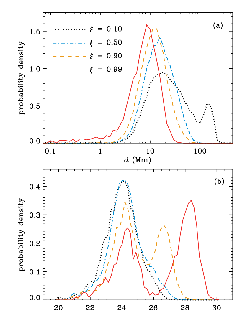
Figure 2: Normalized probability distributions for (a) footpoint separation distance $d$, and (b) estimated free energy $E_{\rm co}$ released by magnetic reconnection in loop-opening events. Four of the six Monte Carlo models are shown for each quantity, with $\xi=0.1$ (black dotted curve), $\xi=0.5$ (blue dot-dashed curve), $\xi=0.9$ (gold dashed curve), $\xi=0.99$ (red solid curve). The other two models ($\xi=0.3$, 0.7) have distributions that fall in between the ones shown.

Figure 2 shows probability distributions for the footpoint separation distance $d$ and the liberated free energy $E_{\rm co}$ associated with the database of loop-opening events output by the Monte Carlo code. For both quantities, the values were collected into 60 discrete histogram bins distributed uniformly in the logarithm of either $d$ or $E_{\rm co}$. The distributions of $d$ values shown in Figure 2(a) have median values that decrease monotonically with increasing $\xi$: from 22.8 Mm ($\xi=0.1$) to 7.89 Mm ($\xi=0.99$). This corresponds closely to the trend seen in maximum loop heights (i.e., 95% percentile values) shown in Figure 7 of Cranmer & van Ballegooijen (2010). The mean and median values of loop height fell below these maximum values, but they followed similar monotonic trends with $\xi$. Below, we consider $d$ to be an approximate upper limit for the loop height during an RLO event; i.e., one can safely evaluate the wave-packet quantities defined in Section 3.1 at heights at or above $d$.

The values of $E_{\rm co}$ shown in Figure 2(b) were computed for a standard assumption of $\theta_{\rm L}C_{\rm L}=0.006$ in Equation (2). This is close to the geometric mean of the two limiting values found by Cranmer & van Ballegooijen (2010) (i.e., 0.003 and 0.011), and it is important to note that the factor of 4 difference between those numbers is only a lower limit to the uncertainty range for this quantity. For most values of $\xi$, the distribution of $E_{\rm co}$ values is single-peaked, with most-probable values in the nanoflare range (i.e., $10^{24}$ erg). However, for cases with $\xi=0.9$ and $\xi=0.99$ there is a marked bimodality, with a second peak reaching up to “microflare” energies. This double-peak structure arises mainly from the distribution of $\Phi_{\rm co}$ fluxes output by the Monte Carlo code, and is only very weakly anticorrelated with the distribution of $d$ values. Cranmer & van Ballegooijen (2010) speculated that these strong ($10^{28}$ erg) events may correspond to the bright polar jets observed in large coronal holes.

Figure 3 shows an example $B_{x}(t)$ waveform for the $\xi=0.7$ model and a subset of the full 10-day coronal simulation time. Magnetic perturbations were computed using a fine sampling timestep of 10 seconds, which resolves individual Gaussian-packet profiles with 30 measurement points per $\Delta t$. In order to compute these waveforms, values needed to be chosen for two remaining parameters: $f_{\rm B}$ and $V_{\rm A}$. For the remainder of this paper, we assume the partition fraction $f_{\rm B}$ has a value of 0.25. This is consistent with roughly half of the released free energy going into an Alfvénic pulse that exhibits equipartition between its kinetic and magnetic energy components (Walén, 1944). The Alfvén speed $V_{\rm A}$ depends on the height at which the waves are simulated. The results presented here assume a representative height $z=100$ Mm above the photosphere, which is above the peaks of nearly all loops but still close enough to the Sun to justify ignoring spherical expansion effects. Self-consistent coronal models based on photosphere-driven waves and turbulence (Cranmer et al., 2007, 2013) give a range of Alfvén speeds at this height between about 1500 and 3200 km s^-1, depending on whether it is a fast or slow solar wind stream. Thus, we adopted a typical value of $V_{\rm A}=2000$ km s^-1.

Figure 3: Summed magnetic perturbation, due to the full set of loop-opening events for the $\xi=0.7$ Monte Carlo model, evaluated at a measurement height of $z=100$ Mm. See text for the values of all input parameters.

Stochastic time-series waveforms can often be understood more clearly when examined in the frequency domain. For each of the six Monte Carlo models, Fast Fourier Transforms (FFTs) were performed on the $B_{x}$ and $B_{y}$ waveforms, and power spectra were computed by multiplying each FFT by its own complex conjugate. Frequency integrals over these power spectra would give the variances $\langle B_{x}^{2}\rangle$ and $\langle B_{y}^{2}\rangle$. Lastly, the sum of these two power spectra, divided by $8\pi$, gives the full transverse magnetic energy power spectrum $P_{\rm B}(f)$. Thus,

$$\frac{\langle B_{x}^{2}\rangle}{8\pi}\,+\,\frac{\langle B_{y}^{2}\rangle}{8\pi}\,=\,\int_{0}^{\infty}df\,\,P_{\rm B}(f)\,=\,U_{\rm B}\,\,,$$ (11)

where $U_{\rm B}$ is the time-averaged magnetic energy density due to transverse fluctuations at the adopted measurement point. Figure 4 shows $P_{\rm B}(f)$ for three of the six Monte Carlo models. These spectra tend to be flat (i.e., “white noise”) for frequencies less than about $2\times 10^{-4}$ Hz, and they begin to drop off exponentially around $10^{-3}$ Hz. All six models have similar spectral shapes, and they all have nearly identical values of the most-probable frequency, defined by

$$\langle f\rangle\,=\,\frac{\int df\,\,P_{\rm B}(f)\,\,f}{\int df\,\,P_{\rm B}(f)}\,\approx\,4.27\times 10^{-4}\,\,\mbox{Hz.}$$ (12)

Among the six models, the standard deviation in $\langle f\rangle$ is only about 3% of the mean value given above. The corresponding most-probable period $\langle f\rangle^{-1}$ is approximately 40 minutes.

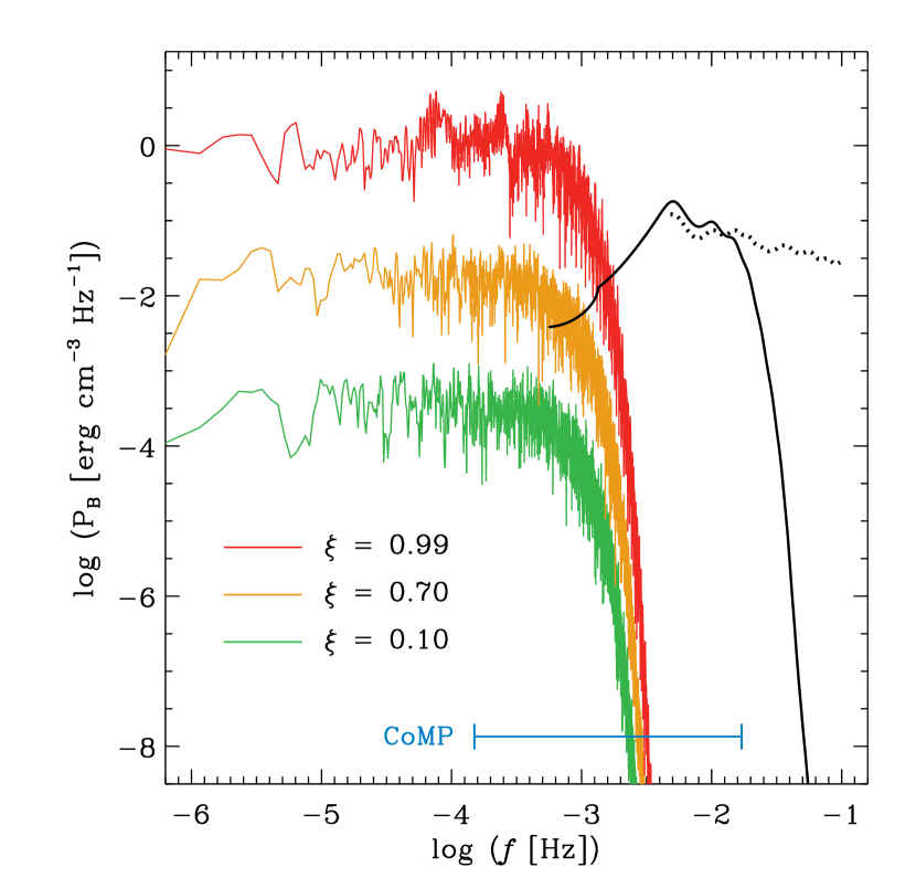
Figure 4: Magnetic energy density power spectra for RLO Monte Carlo models with $\xi=0.1$ (green curve), $\xi=0.7$ (gold curve), and $\xi=0.99$ (red curve). Also shown are Alfvénic fluctuation spectra driven by photospheric motions and extrapolated up to $z=100$ Mm, from the idealized coronal-hole model of Cranmer & van Ballegooijen (2005) (solid black curve) and the measurements of Chitta et al. (2012) (dotted black curve). The range of frequencies measured by CoMP (horizontal blue bar) is also noted.

The computed spectral shapes can be understood as a manifestation of the assumed pulse shapes shown in Figure 3. Cranmer & van Ballegooijen (2005) showed that the power spectrum corresponding to a series of intermittent Gaussian pulses is given by

$$P_{\rm B}\,\propto\,e^{-2\pi^{2}\tau^{2}f^{2}}$$ (13)

where $\tau$ is the $1/e$ half-width of a single pulse measured at a fixed location in space. This is essentially the same quantity as the timestep $\Delta t$ used in Equation (9). Thus, it is not surprising that the above expression, with $\tau=5$ min, is an excellent fit to the frequency dependence of the curves shown in Figure 4. In addition, Equation (13) provides an exact solution for the most-probable frequency,

$$\langle f\rangle\,=\,\frac{1}{\tau\sqrt{2\pi^{3}}}$$ (14)

which also agrees well with the numerical solutions to Equation (12) discussed above. Of course, in the real corona, there must be a continuous distribution of reconnection timescales instead of a single $\Delta t$, so we expect the resulting power spectra to drop off more gradually with increasing frequency.

For comparison, Figure 4 also shows power spectra that estimate the coronal magnitudes of MHD waves driven by photospheric granulation. The two black curves were derived from horizontal kinetic energy spectra that in turn were computed from intergranular bright-point motions—one of them from a semianalytic model based on earlier observations (Cranmer & van Ballegooijen, 2005), and the other from more recent high-resolution data (Chitta et al., 2012). The processing of the latter data was discussed in more detail by Van Kooten & Cranmer (2017), who also found a similar high-frequency power-law tail in spectra derived from simulations. These photospheric spectra were extrapolated up to a coronal height of $z=100$ Mm and converted to magnetic fluctuation spectra using the polar coronal-hole model of Cranmer & van Ballegooijen (2005).

The dominant frequencies of the photospheric waves shown in Figure 4 tend to be much higher than those produced by the Monte Carlo reconnection model. However, there is a region of frequency overlap in which both models may contribute comparably to the total power. In this region, the Monte Carlo model shows decreasing power as a function of increasing frequency, and the Cranmer & van Ballegooijen (2005) model shows increasing power as a function of increasing frequency. The latter can be understood by examining the propagation history of these waves from the photosphere to the corona. Waves near the peak of the black curve ($\log f\approx-2.3$) are above the photospheric kink-mode cutoff frequency, so they have been propagating the whole way. Waves at the low-frequency end of the Cranmer & van Ballegooijen (2005) spectrum ($\log f\approx-3.3$) spent some time below the kink-mode cutoff in the low chromosphere. Thus, they experienced some evanescent decay and ended up with less power in the corona.

The region of frequency overlap between the two sets of models in Figure 4 corresponds to the frequencies measured by the Coronal Multi-channel Polarimeter (CoMP; Tomczyk et al., 2008). Although CoMP measurements so far do not yet allow us to measure the absolute wave power in the corona (mainly because of line-of-sight cancellation of overlapping Doppler signals), they have provided useful data on the shape of the Alfvén-wave power spectrum. Between frequencies of $10^{-4}$ and $10^{-2}$ Hz, CoMP tends to show monotonically decreasing power with slopes of order $P\propto f^{-1}$ to $f^{-1.5}$ (Tomczyk & McIntosh, 2009; Liu et al., 2014; Morton et al., 2016). Figure 4 indicates that an understanding of this monotonic spectrum may require us to take account of both the low-frequency reconnection-driven waves and the high-frequency photospheric waves.

The remainder of this paper discusses the magnitudes of the reconnection-generated waves shown in Figure 4. The magnetic energy density $U_{\rm B}$, as defined in Equation (11), varies by more than three orders of magnitude from the $\xi=0.1$ model ($U_{\rm B}=2.7\times 10^{-7}$ erg cm^-3) to the $\xi=0.99$ model ($U_{\rm B}=9.7\times 10^{-4}$ erg cm^-3). This relative increase can be understood by examining the scaling for the magnetic perturbation due to a single reconnection pulse. Using Equations (2), (8), and (10)—and ignoring quantities that remain unchanged from one value of $\xi$ to another—one can estimate

$$U_{\rm B}\,\propto\,\frac{\Phi_{\rm co}B_{\rm net}}{d}\,\,.$$ (15)

Cranmer & van Ballegooijen (2010) showed that $B_{\rm net}$ increases by about a factor of 90 as $\xi$ increases from 0.1 to 0.99. Note that $B_{\rm net}=\xi B_{\rm abs}$, and $B_{\rm abs}$ increases with $\xi$ because the more unipolar models tend to have a faster emergence rate of flux elements into the photosphere. The statistical quantities output from the Monte Carlo model (as shown in Figure 2) indicate that the mean ratio $\Phi_{\rm co}/d$ increases by about a factor of 60 as $\xi$ increases from 0.1 to 0.99. Thus, Equation (15) predicts a factor of 5400 increase in $U_{\rm B}$ over this range. This slightly overestimates the factor of 3600 seen in the numerical models, but Equation (15) is only a simple approximation. For example, it does not take into account the effect of temporal intermittency for multiple pulses sampled by a fixed observer.

Figure 5 shows an estimate of the radial dependence of each model’s wave energy density $U_{\rm B}$. For the Monte Carlo models, these curves were computed by assuming the wave energy is built up gradually over the heights corresponding to each model’s distribution of footpoint separation distances $d$. In other words, a loop-opening event with footpoint separation $d$ is assumed to deposit its free energy as upward-propagating waves only at heights $z\geq d$. Thus, the radial functions shown in Figure 5 are the integrated (cumulative) distributions that correspond to the probability distributions shown in Figure 2(a). Each curve was then normalized to that model’s own value of $U_{\rm B}$.

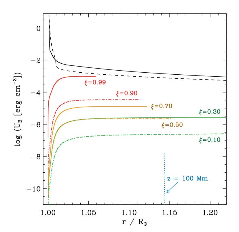
Figure 5: Radial dependence of magnetic energy densities $U_{\rm B}$ of coronal waves. Results from the Monte Carlo models (red, gold, and green curves) were computed as described in the text. Models of high-frequency photosphere-generated waves were taken from Cranmer & van Ballegooijen (2005) (solid black curve) and Cranmer et al. (2007) (dashed black curve).

Figure 5 also shows the known radial dependence of magnetic fluctuation energy density for the photosphere-driven wave models of Cranmer & van Ballegooijen (2005) and Cranmer et al. (2007). This radial dependence is derived from wave-action conservation, which in the low corona works out to the proportionality $U_{\rm B}\propto\rho^{1/2}$. At large distances, the Monte Carlo models also ought to exhibit a similar radial decline in $U_{\rm B}$ as do the photosphere-driven waves, but that effect was not included in the multi-color curves shown in Figure 5. All of the modeled reconnection-driven waves (except the extreme case $\xi=0.99$) have energy densities substantially weaker than those corresponding to the higher-frequency MHD waves expected to come from the photosphere.

4 Non-WKB Properties of the Waves

Although MHD waves associated with magnetic-carpet reconnection do not appear to dominate the total wave energy density in the corona, they may be responsible for “filling in” the lowest frequencies of the power spectrum. In interplanetary space, the highest power levels occur at the lowest frequencies (see, e.g., Tu & Marsch, 1995; Bruno & Carbone, 2013). It is still not known what fraction of these low-frequency fluctuations originates in the corona (or lower), what fraction is produced by some kind of inverse cascade from the high-frequency turbulence, and what fraction may be the result of corotating (but otherwise time-steady) flux tubes advecting past the spacecraft.

Remote-sensing observations can be used to put constraints on the properties of the coronal MHD-wave spectrum. Emission-line spectroscopy provides information about long-time averages of transverse velocity fluctuations via the so-called “nonthermal” component of the line profile (Boland et al., 1973; Mariska et al., 1979). This information is complementary to the short-time Doppler fluctuations measured by, e.g., CoMP, as discussed above. Measurements made above coronal holes over the past few decades (Tu et al., 1998; Banerjee et al., 1998; Cranmer & van Ballegooijen, 2005; Dolla & Solomon, 2008; Landi & Cranmer, 2009) appeared to agree well with theoretical predictions of undamped Alfvén waves launched at the solar surface. However, more recent data from the Extreme-ultraviolet Imaging Spectrometer (EIS) on Hinode seem to show substantial wave damping above heights of roughly 0.2 $R_{\odot}$ (Hahn et al., 2012; Bemporad & Abbo, 2012; Hahn & Savin, 2013; Gupta, 2017).

There is still no universally agreed-upon explanation for the apparent wave damping inferred from EIS observations. Undamped WKB Alfvén waves require a radial increase in their transverse velocity amplitude ($v_{\perp}\propto\rho^{-1/4}$), but the data show nonthermal line-widths flattening out and possibly starting to decrease with increasing height. This may be indicative of some actual wave dissipation (Zhao et al., 2015), but it also disagrees with earlier models that predicted much weaker damping in the corona (see, e.g., Cranmer et al., 2017). It also disagrees with earlier measurements of larger nonthermal line widths at heights just barely above those probed by EIS (Esser et al., 1999). Earlier studies ruled out contamination by instrumental stray light—which would add a narrower component to the broad coronal emission line—but more recent work indicates EIS sometimes sees a stray-light signal several times stronger than was assumed previously (Wendeln & Landi, 2018). Also, the traditional assumption that emission-line profiles are dominated by motions in the “plane of the sky” may not be valid for all ions. A given ion’s transition from ionization equilibrium at low heights to frozen-in ionization at large heights needs to be modeled self-consistently in order to determine the regions that dominate the observed line profile (see, e.g., Gilbert & Cranmer, 2018).

This paper provides another possible explanation for the observational data: departures from Walén (1944) energy equipartition. This would be a natural consequence of the extremely low-frequency spectrum associated with reconnection-driven waves. High-frequency MHD fluctuations are expected to have wavelengths smaller than the scales of radial variation in the corona. Thus, they should behave as ideal WKB waves in a homogeneous background, with equal magnetic and kinetic energy densities ($U_{\rm B}=U_{\rm K}$). On the other hand, studies of non-WKB wave propagation (e.g., Heinemann & Olbert, 1980; Barkhudarov, 1991; MacGregor & Charbonneau, 1994) tend to show how low-frequency (large-wavelength) waves become reflected by the radial variations and exhibit $U_{\rm B}>U_{\rm K}$. It is worthwhile to note that the MHD simulations of Lynch et al. (2014) also saw $U_{\rm B}>U_{\rm K}$ for transient fluctuations driven by reconnection. With less of the total energy going into kinetic fluctuations, the observable transverse velocity amplitude $v_{\perp}$ would be lower than in the WKB limit.

Figure 6(a) shows what the root-mean-squared (rms) Alfvén-wave velocity amplitudes would look like for a range of monochromatic frequencies. Each curve is assumed to have the same radial variation of $U_{\rm tot}=U_{\rm B}+U_{\rm K}$, but the Alfvén ratio $\alpha=U_{\rm K}/U_{\rm B}$ is different for each frequency. The radial dependences of both $U_{\rm tot}$ and $\alpha$ are taken from the non-WKB models of Cranmer & van Ballegooijen (2005). Thus, for each curve, the velocity amplitude is computed from

$$v_{\perp}^{2}\,=\,\frac{2U_{\rm K}}{\rho}\,=\,\frac{2U_{\rm tot}}{\rho}\,\left(\frac{\alpha}{1+\alpha}\right)\,\,.$$ (16)

The plotted velocities were also multiplied by $1/\sqrt{2}$ in order to show just one projected transverse component. This allows a more direct comparison with the observed nonthermal line-widths. For the shortest periods, $\alpha\approx 1$ and the curves resemble the classical WKB result ($v_{\perp}\propto\rho^{-1/4}$). For the longest periods, the curves flatten out in a manner similar to what is seen in the observations.

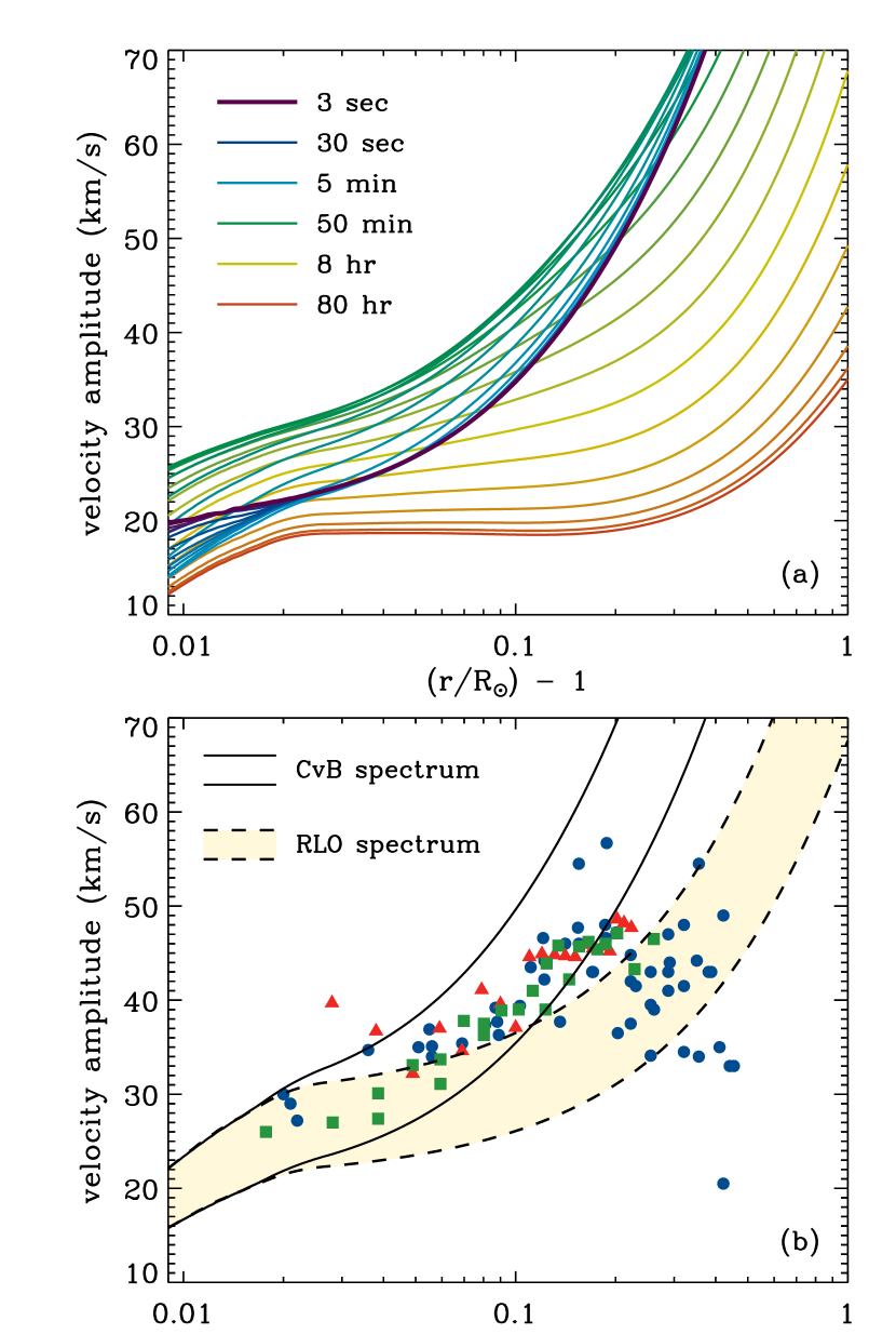
Figure 6: Line-of-sight projected Alfvén-wave velocity amplitudes. (a) Curves computed for 31 discrete wave periods sampled from an evenly spaced logarithmic grid from 0.05 to 5000 min. Legend shows one color per decade in period. (b) Observed nonthermal speeds from Banerjee et al. (1998, green squares), Landi & Cranmer (2009, red triangles), and Hahn & Savin (2013, blue circles). Weighted averages are shown using power spectra from Cranmer & van Ballegooijen (2005) (solid curves) and Monte Carlo results of this paper (dashed curves).

Figure 6(b) shows observed coronal-hole data points from Banerjee et al. (1998), Landi & Cranmer (2009), and Hahn & Savin (2013). The curves indicate weighted-average velocity amplitudes computed by integrating over a power spectrum, with

$$\langle v_{\perp}^{2}\rangle\,=\,\frac{2}{\rho}\int_{0}^{\infty}df\,\,P_{\rm B}(f)\,\alpha(f)\,\,.$$ (17)

These curves are presented in pairs, with one multiplied by $1/\sqrt{2}$ as discussed above, and the other left alone. This is meant to illustrate the observed spread in the data, some of which may be due to intrinsic variability in the wave-generation regions (e.g., plumes versus interplume regions in coronal holes). The solid curves were computed from the high-frequency-dominated photosphere-driven spectrum of Cranmer & van Ballegooijen (2005), which tends to resemble the WKB limiting case of $v_{\perp}\propto\rho^{-1/4}$.

The dashed curves in Figure 6(b) were computed using a somewhat speculative hypothesis that the wave magnitudes obey the same radial dependence of $U_{\rm tot}$ used in Figure 6(a), but the power spectrum is that of the reconnection-driven waves as shown in Figure 4 and estimated in Equation (13). Of course, the Monte Carlo model predicts that only a small fraction of the total power is in the form of these low-frequency reconnection-driven waves. However, it is possible that the development of coronal turbulence drives the spectral shape towards one dominated by the lowest frequencies. In this case, the energy partition becomes dominated by the magnetic fluctuations (i.e., $U_{\rm B}>U_{\rm K}$) and the velocity amplitude flattens out between heights of 0.05 and 0.30 $R_{\odot}$ in a manner somewhat reminiscent of the EIS data.

5 Discussion and Conclusions

This paper took the output from an existing Monte Carlo model of the Sun’s magnetic carpet (Cranmer & van Ballegooijen, 2010) and used it to simulate the properties of low-frequency MHD waves generated by multiple magnetic reconnection events. In most regions of mixed magnetic polarity (i.e., everywhere except the most unipolar regions typified by the $\xi=0.99$ models), the total power in reconnection-driven waves is predicted to be much lower than the power in waves associated with photospheric granulation. However, the reconnection-driven waves may dominate the coronal power spectrum at frequencies lower than $10^{-4}$ to $10^{-3}$ Hz. Thus, obtaining a complete understanding of the turbulent power observed by off-limb instruments such as CoMP (Tomczyk & McIntosh, 2009) may be predicated on improving our knowledge about reconnection-generated MHD waves.

The results presented in this paper represent only a cursory survey of the actual properties of reconnection-driven waves in the corona. This work needs to be followed by more comprehensive models and more focused comparisons to the observations. For example, note that the original Cranmer & van Ballegooijen (2010) Monte Carlo model was created to address the issue of whether RLO-type events could be responsible for accelerating the solar wind. Thus, most of the focus has been on $E_{\rm co}$, the energy in “closed-to-open” reconnection events. Cranmer & van Ballegooijen (2010) found that there also occur “open-to-closed” type events that have mean energies $E_{\rm oc}$ roughly comparable to $E_{\rm co}$. These events may produce downward-propagating waves, which have been seen in simulations (e.g., Lynch et al., 2014) and may be an important source of counterpropagating wave packets as needed for the production of a turbulent cascade (Iroshnikov, 1963; Kraichnan, 1965; Howes & Nielson, 2013).

The Cranmer & van Ballegooijen (2010) simulations also did not keep track of “closed-to-closed” reconnection events; i.e., those that involve swapping footpoints between neighboring closed-loop flux systems. Those kinds of events may dominate the energy budget at low heights in regions of mixed magnetic polarity. Candelaresi et al. (2016) discussed how a sufficiently complex coronal field-line topology can trap MHD waves and cause stresses to build up in magnetically closed regions. However, if an appreciable fraction of reconnection-driven waves are in compressible modes that transmit energy across the field, then some of that energy may ultimately escape into the solar wind. In fact, simulations often show that reconnection can give rise to fast/slow magnetosonic modes (e.g., Kigure et al., 2010) as well as torsional Alfvénic pulses that resemble flux ropes (Higginson & Lynch, 2018).

Some other limitations of the Cranmer & van Ballegooijen (2010) Monte Carlo model were listed at the end of Section 2. There is also the sensitivity of the modeled wave power to the presumed energy partition fraction $f_{\rm B}$, which was only estimated qualitatively. Many of these limitations could be addressed by replacing this kind of model by a fully three-dimensional solution of the MHD conservation equations (see, e.g., Amari et al., 2015; Carlsson et al., 2016; Rempel, 2017; Martínez-Sykora et al., 2017). However, an MHD simulation that would encompass the region shown in Figure 1—and run it for several days of physical time—remains extremely computationally expensive. Semi-analytic techniques allow us to simulate the required domains with both modest resources and more-than-adequate dynamic range (in space and time).

Lastly, it remains to be seen whether the proposed reconnection-driven waves are responsible for either: (1) the unexpectedly narrow Hinode/EIS line profiles, or (2) the low-frequency-dominated turbulent power spectra measured in interplanetary space. For the former, it would be advantageous to repeat the measurements with a properly occulted coronagraph spectrometer, such as a next-generation follow-on to the SOHO Ultraviolet Coronagraph Spectrometer (see, e.g., Kohl et al., 2008). For the latter, it was mentioned above that much of the low-frequency variability observed in situ may be due to the Sun’s rotation carrying uncorrelated bundles of magnetic flux past the spacecraft. If these fluctuations are similar to larger-scale corotating interaction regions (CIRs), they may be distinguishable from Alfvén waves from their strong variations in magnetic pressure (Cranmer et al., 2013). It would also be advantageous to measure solar wind fluctuations from a spacecraft in strict corotation with the plasma. Parker Solar Probe (PSP) will spend a few days near corotation around each perihelion (Fox et al., 2016) but probably not long enough to gather sufficient data to probe the $f<10^{-4}$ Hz part of the spectrum.

References

- Alfvén (1947) Alfvén, H. 1947, MNRAS, 107, 211
- Amari et al. (2015) Amari, T., Luciani, J.-F., & Aly, J.-J. 2015, Nature, 522, 188
- Antiochos et al. (2011) Antiochos, S. K., Mikić, Z., Titov, V., et al. 2011, ApJ, 731, 112
- Anusha et al. (2017) Anusha, L. S., Solanki, S. K., Hirzberger, J., & Feller, A. 2017, A&A, 598, A47
- Axford & McKenzie (1992) Axford, W. I., & McKenzie, J. F. 1992, in Solar Wind Seven, ed. E. Marsch & R. Schwenn (New York: Pergamon), 1
- Banerjee et al. (1998) Banerjee, D., Teriaca, L., Doyle, J. G., & Wilhelm, K. 1998, A&A, 339, 208
- Barkhudarov (1991) Barkhudarov, M. R. 1991, Sol. Phys., 135, 131
- Bemporad & Abbo (2012) Bemporad, A., & Abbo, L. 2012, ApJ, 751, 110
- Beveridge & Longcope (2006) Beveridge, C., & Longcope, D. W. 2006, ApJ, 636, 453
- Birn et al. (2009) Birn, J., Fletcher, L., Hesse, M., & Neukirch, T. 2009, ApJ, 695, 1151
- Boland et al. (1973) Boland, B. C., Engstrom, S. F. T., Jones, B. B., & Wilson, R. 1973, A&A, 22, 161
- Brannon et al. (2015) Brannon, S. R., Longcope, D. W., & Qiu, J. 2015, ApJ, 810, 4
- Bruno & Carbone (2013) Bruno, R., & Carbone, V. 2013, Living Rev. Solar Phys., 10, 2
- Candelaresi et al. (2016) Candelaresi, S., Pontin, D. I., & Hornig, G. 2016, ApJ, 832, 150
- Carlsson et al. (2016) Carlsson, M., Hansteen, V. H., Gudiksen, B. V., et al. 2016, A&A, 585, A4
- Chitta et al. (2012) Chitta, L. P., van Ballegooijen, A. A., Rouppe van der Voort, L., et al. 2012, ApJ, 752, 48
- Cirtain et al. (2007) Cirtain, J. W., Golub, L., Lundquist, L., et al. 2007, Science, 318, 1580
- Close et al. (2005) Close, R. M., Parnell, C. E., Longcope, D. W., & Priest, E. R. 2005, Sol. Phys., 231, 45
- Close et al. (2003) Close, R. M., Parnell, C. E., Mackay, D. H., & Priest, E. R. 2003, Sol. Phys., 212, 251
- Cossette & Rast (2016) Cossette, J.-F., & Rast, M. P. 2016, ApJ, 829, L17
- Cranmer et al. (2017) Cranmer, S. R., Gibson, S. E., & Riley, P. 2017, Space Sci. Rev., 212, 1345