Coscattering/Coannihilation Dark Matter in a Fraternal Twin Higgs Model
Abstract
Dark matter candidates arise naturally in many models that address the hierarchy problem. In the fraternal twin Higgs model which could explain the absence of the new physics signals at the Large Hadron Collider (LHC), there are several viable dark matter candidates. In this paper we study the twin neutrino in the mass range 0.1–10 GeV as the dark matter. The thermal relic density is determined by the interplay of several annihilation and scattering processes between the twin neutrino, twin tau, and twin photon, depending on the order of the freeze-out temperatures of these processes. Besides the common coannihilation scenario where the relic density is controlled by the twin tau annihilation, it can realize the recently discovered coscattering phase if the scattering of the twin neutrino into the twin tau freezes out earlier than the twin tau annihilation. We also provide a method to calculate the thermal relic density in the intermediate regime where both coannihilation and coscattering processes contribute to the determination of the dark matter density. We show that the right amount of dark matter can be obtained in various scenarios in different regions of the parameter space. The current experimental constraints and future probes into the parameter space from direct detections, cosmological and astrophysical bounds, dark photon searches, and displaced decays at colliders, are discussed.
I Introduction
The hierarchy problem and the dark matter are two main motivations for new physics near the electroweak (EW) scale. In the standard model (SM), the Higgs field receives large quadratically divergent contributions to its potential from the interactions with SM particles, in particular, the top quark and weak gauge bosons. For a natural EW symmetry breaking scale, new particles are expected to be close to the EW scale to cut off these quadratic contributions. On the other hand, a stable weakly interacting massive particle (WIMP) with a mass around the EW scale gives a right amount of thermal relic from the Hot Big Bang to account for the dark matter in the universe. It is called “WIMP miracle.” Such a dark matter particle candidate also often appears naturally in models which address the hierarchy problem. The most popular and most studied examples are the supersymmetric (SUSY) extensions of SM. With a conserved -parity, the lightest neutralino is stable and represents a good dark matter candidate. The models that can explain both the hierarchy problem and dark matter are particularly attractive because they provide a link between the two mysterious problems.
The new particles related to the hierarchy problem and the WIMPs have been extensively searched at various experiments. So far none of them has been discovered. The LHC has put very strong bounds on new colored particles that can cancel the SM top loop contribution to the Higgs mass. Except for some special cases, the bounds on the masses of new colored particles generically exceed 1 TeV. This would imply a quite severe tuning of the Higgs mass if the top loop is not canceled below 1 TeV. Direct searches of DM also put strong bounds on the scattering cross sections of the DM particle with nucleons. A big fraction of the expected region of the WIMP parameter space from typical SUSY models is excluded, though there are still surviving scenarios. These null experimental results have prompted people to wonder that the standard pictures such as SUSY might not be realized at the electroweak scale in nature. Alternative solutions to the hierarchy problem and DM where the interactions between new particles and SM particles are stealthier should be taken more seriously.
For the hierarchy problem, the “neutral naturalness” models gained increasing attentions in recent years. In these models, the top quark partners which regularize the top loop contribution to the Higgs mass do not carry SM color quantum numbers, and hence are not subject to the strong bounds from the LHC. The mirror twin Higgs model Chacko:2005pe is the first example and is probably the stealthiest one. The twin sector particles are SM singlets but charged under their own gauge group. They are related to the SM sector by a symmetry. As a result, the mass terms of the Higgs fields of the SM and twin sectors exhibit an enhanced symmetry. The 125 GeV Higgs boson arises as a pseudo-Nambu-Goldstone boson (PNGB) of the spontaneously broken symmetry. The twin sector particles are difficult to produce at colliders because they do not couple to SM gauge fields. The main experimental constraints come from the mixing between the SM Higgs and the twin Higgs, which are rather weak. The model can still be natural without violating current experimental bounds.
The next question is whether the neutral naturalness models like the twin Higgs possess good dark matter candidates. In the fraternal version of the twin Higgs model Craig:2015pha , people have shown that there are several possible dark matter candidates Garcia:2015loa ; Craig:2015xla ; Garcia:2015toa ; Farina:2015uea . The fraternal twin Higgs takes a minimal approach in addressing the hierarchy problem using the twin Higgs mechanism. In this model, the twin fermion sector only contains the twin partners of the third generation SM fermions, since only the top Yukawa coupling gives a large contribution to the Higgs mass that needs to be regularized below the TeV scale. The twin gauge boson can be absent or can have a mass without affecting the naturalness. The fraternal twin Higgs model can avoid potential cosmological problems of an exact mirror twin Higgs model which contains many light or massless particles in the twin sector. Refs. Garcia:2015loa ; Craig:2015xla showed that the twin tau can be a viable dark matter candidate. The correct relic density is obtained for a twin tau mass in the range of 50–150 GeV, depending on other model parameters. If twin hypercharge is gauged, then the preferred mass is lighter, in the 1–20 GeV range Craig:2015xla . Another possibility is asymmetric dark matter from the twin baryon made of twin -quarks, where the relic density is set by the baryon asymmetry in the twin sector Garcia:2015toa ; Farina:2015uea .
In this paper, we explore a new scenario where the dark matter is the twin neutrino, in the mass range 0.1–10 GeV. In previous studies of twin tau dark matter, its stability is protected by the twin symmetry, which is assumed to be a good symmetry, either gauged or global. Here we consider that the twin is broken so that the twin photon acquires a mass to avoid potential cosmological problems. In this case, the twin tau and the twin neutrino can mix so the twin tau can decay to the twin neutrino if the twin tau is heavier. The twin neutrino, on the other hand, being the lightest twin fermion, can be stable due to the conservation of the twin lepton number or twin lepton parity. An interesting scenario is that if the twin photon, twin neutrino, and twin tau all have masses of the same order around a few GeV or below, the right amount of dark matter relic density from twin neutrinos can be obtained. The relic density is controlled by the coannihilation and recently discovered coscattering processes DAgnolo:2017dbv ; Garny:2017rxs .
The coscattering phase is considered as the fourth exception in the calculation of thermal relic abundances in addition to the three classical cases enumerated in Ref. Griest:1990kh . It is closely related to the coannihilation case as both require another state with mass not far from the dark matter mass so that the partner state can play an important role during decoupling. The difference is that in the coannihilation phase the relic density is controlled by the freeze-out of the annihilation processes of these particles, while in coscattering phase the relic density is controlled by the freeze-out of the inelastic scattering of a dark matter particle into the partner state. Because of the energy threshold of the upward scattering, the coscattering process has a strong momentum dependence. This makes the relic density calculation quite complicated. The standard DM calculation tools such as micrOMEGAs Belanger:2018ccd , DarkSUSY Bringmann:2018lay , and MadDM Ambrogi:2018jqj do not apply and one needs to solve the momentum-dependent Boltzmann equations. Also, because of the momentum dependence of the coscattering process, we find that there are parameter regions of mixed phase, i.e., the relic abundance is controlled partially by coannihilation and partially by coscattering. We investigate in detail the relevant parameter space and perform calculations of the relic abundance in different phases, including situations where it is controlled by coannihilation, by coscattering, or by both processes. The calculation in the mixed phase is more involved and we discuss a relatively simple method to obtain the DM abundance with good accuracies.
The twin neutrino DM does not couple to SM directly. Its couplings to matter through mixings of the photons or the Higgses between the SM sector and the twin sector are suppressed, so the direct detection experiments have limited sensitivities. Some of the main constraints come from indirect detections and searches of other associated particles. Its annihilation through twin photon is constrained by Cosmic Microwave Background (CMB), 21cm line absorption, and Fermi-LAT data. For associated particles, the light dark photon searches provide some important constraints and future probes.
The paper is organized as follows. In Sec. II we first give a brief summary of the fraternal twin Higgs model and its possible DM candidates. Then we focus the discussion on the sector of our DM scenario, i.e., the twin neutrino as the DM, and its coannihilation/coscattering partners, the twin tau and the twin photon. In Sec. III we enumerate the relevant processes and discuss their roles in controlling the DM abundance in different scenarios. Sec. IV describes how to evaluate the DM relic density in different phases, including the coannihilation phase, the coscattering phase, and the mixed phase. Some details about the calculations are collected in the Appendices. Our numerical results for some benchmark models are presented in Sec. V. In Sec. VI we discuss various experimental constraints and future probes of this DM scenario. The conclusions are drawn in Sec. VII.
II Fraternal Twin Higgs and Light DM
The twin Higgs model postulates a mirror (or twin) sector which is related to the SM sector by a symmetry. The particles in the twin sector are completely neutral under the SM gauge group but charged under the twin gauge group. Due to the symmetry, the Higgs fields of the SM sector and the twin sector exhibit an approximate (or ) symmetry. The symmetry is spontaneously broken down to by the Higgs vacuum expectation values (VEVs). A phenomenological viable model requires that the twin Higgs VEV to be much larger than the SM Higgs VEV , , so that the light uneaten pseudo-Nambu-Goldstone boson (pNGB) is an SM-like Higgs boson. (The other six Nambu-Goldstone bosons are eaten and become the longitudinal modes of the bosons of the SM sector and the twin sector.) This requires a small breaking of the symmetry. The one-loop quadratically divergent contribution from the SM particles to the Higgs potential is cancelled by the twin sector particles, which are heavier than their SM counterparts by the factor of . The model can be relatively natural for .
The twin sector particles are not charged under the SM gauge group so it is difficult to look for them at colliders. However, if there is an exact mirror content of the SM sector and the couplings respect the symmetry, there will be light particles (photon, electron, neutrinos) in the twin sector. They can cause cosmological problems by giving a too big contribution to .111Some solutions within the mirror twin Higgs framework can be found in Refs. Farina:2015uea ; Chacko:2016hvu ; Craig:2016lyx ; Barbieri:2016zxn ; Csaki:2017spo ; Barbieri:2017opf . In addition, in general one expects a kinetic mixing between two gauge fields. If the twin photon is massless, its kinetic mixing with the SM photon is strongly constrained. On the other hand, these light particles have small couplings to the Higgs and hence play no important roles in the hierarchy problem. One can take a minimal approach to avoid these light particles by only requiring the symmetry on the parts which are most relevant for the hierarchy problem. This is the fraternal twin Higgs (FTH) model proposed in Ref. Craig:2015pha . The twin sector of the FTH model can be summarized below.
-
•
The twin and gauge couplings should be approximately equal to the SM and gauge couplings. The twin hypercharge does not need to be gauged. If it is gauged, its coupling can be different from the SM hypercharge coupling, as long as it is not too big to significantly affect the Higgs potential. Also, the twin photon can be massive by spontaneously breaking the gauge symmetry or simply writing down a Stueckelberg mass term.
-
•
There is a twin Higgs doublet. Together with the SM Higgs doublet there is an approximate -invariant potential. The twin Higgs doublet acquires a VEV , giving masses to the twin weak gauge bosons and twin fermions.
-
•
The twin fermion sector contains the third generation fermions only. The twin top Yukawa coupling needs to be equal to the SM top Yukawa coupling to a very good approximation so that their contributions to the Higgs potential can cancel. The twin bottom and twin leptons are required for anomaly cancellation, but their Yukawa couplings do not need to be equal to the corresponding ones in the SM, as long as they are small enough to not generate a big contribution to the Higgs potential.
The collider phenomenology of the FTH model mainly relies on the mixing of the SM and twin Higgs fields. In typical range of the parameter space, one often expects displaced decays that constitute an interesting experimental signature. Here we focus on the DM. A natural candidate is the twin tau. Since its Yukawa coupling needs not to be related to the SM tau Yukawa coupling, its mass can be treated as a free parameter. It is found that a right amount of thermal relic abundance can be obtained for a twin tau mass in the range of 50–150 GeV if the twin hypercharge is not gauged Garcia:2015loa ; Craig:2015xla . It corresponds to a twin tau Yukawa coupling much larger than the SM tau Yukawa coupling. The requirement that the twin tau Yukawa coupling does not reintroduce the hierarchy problem puts a upper limit GeV on the twin tau mass. A twin tau lighter than GeV would generate an overabundance which overcloses the universe. The relic density can be greatly reduced if a light twin photon also exists, because it provides additional annihilation channels for the twin tau. If the twin photon coupling strength is similar to the SM photon coupling, the annihilation will be too efficient and it will be difficult to obtain enough DM. For a twin photon coupling , a right amount of relic density can be obtained for a twin tau mass in the range of 1–20 GeV Craig:2015xla .
In the twin tau DM discussion, its stability is assumed to be protected by the twin symmetry. However, if twin is broken and the twin photon has a mass, the twin tau may be unstable and could decay to the twin neutrino if the twin neutrino is lighter. This is because that the twin tau and the twin neutrino can mix due to the twin breaking effect. On the other hand, if the twin lepton number (or parity) is still a good symmetry, the lightest state that carries the twin lepton number (parity) will be stable. In this paper we will assume that it is the twin neutrino and consider its possibility of being the DM.
II.1 Twin lepton mixings
If the twin (or equivalently twin hypercharge) is broken, it is possible to write down various Dirac and Majorana masses between the left-handed and right-handed twin tau and twin neutrino fields. For simplicity, we consider the case where the twin lepton number remains a good symmetry, which can be responsible for the stability of DM. This forbids the Majorana mass terms.
The twin tau and twin neutrino receive the usual Dirac masses from the twin Higgs VEV,
| (1) | |||||
where the subscript represents the twin sector fields, and transforms as under the twin gauge group. The twin hypercharge breaking can be parameterized by a spurion field which is a singlet under but carries twin hypercharge (also twin electric charge). It can come from a VEV of a scalar field which breaks spontaneously. The radial component is assumed to be heavier than the relevant particles (twin photon, tau, and neutrino) here and plays no role in the following discussion. Using the spurion we can write down the following additional lepton-number conserving mass terms,
| (2) |
The mass matrix of the twin tau and twin neutrino is then given by
| (8) |
where
| (9) |
The mass matrix can be diagonalized by the rotations
| (22) |
where the mass eigenstates in the twin sector are labelled with a hat ( ). We assume that the off-diagonal masses so that the mixing angles are small. This is reasonable given that arise from higher dimensional operators and require an insertion of the twin hypercharge breaking VEV, which is assumed to be small for a light twin photon. For our analysis, to reduce the number of independent parameters, we further assume that one of the off-diagonal masses dominates, i.e., , so that we can ignore . In this case, we obtain two Dirac mass eigenstates and which are labeled by their dominant components. The two mass eigenvalues are
| (23) |
and the two mixing angles are given by
| (24) |
in the small mixing angle limit. There is no qualitative difference in our result if and are comparable except that the two mixing angles become independent.
We are interested in the region of parameter space where the twin tau , twin neutrino , and twin photon have masses of the same order in the range GeV, with . Compared with Ref. DAgnolo:2017dbv , the twin neutrino plays the role of which is the DM, corresponds to , the coannihilation/coscattering partner of the DM particle, and corresponds to the mediator . Following Ref. DAgnolo:2017dbv , we define two dimensionless parameters,
| (25) |
which are convenient for our discussion. The region of interest has and .
The mass spectrum and mixing pattern would be more complicated if Majorana masses for the twin leptons are allowed. In addition to the standard Majorana mass for the right-handed twin neutrino, all other possible terms can arise from higher dimensional operators with insertions of the spurion field (and the twin Higgs field ), filling the mass matrix of . There are four mass eigenstates and many more mixing angles. The stability of the lightest eigenstate can be protected by the twin lepton parity in this case. Because the twin photon couples off-diagonally to Majorana fermions, the analysis of annihilation and scattering needs to include all four fermion eigenstates, which becomes quite complicated. Nevertheless, one can expect that there are regions of parameter space where the correct relic abundance can be obtained through coannihilation and/or coscattering processes in a similar way to the case studied in this work.
III Relevant Processes for the Thermal Dark Matter Abundance
At high temperature, the SM sector and the twin sector stay in thermal equilibrium through the interactions due to the Higgs mixing and the kinetic mixing of the gauge fields. As the universe expands, the heavy species in the twin sector decouple from the thermal bath and only the light species including twin photon (), twin tau (), and twin neutrino () survive. These light species talk to SM mainly via the kinetic mixing term, , between and . We assume that the kinetic mixing is big enough () to keep the twin photon in thermal equilibrium by scattering off light SM leptons DAgnolo:2017dbv during the DM freeze-out. The DM abundance is then controlled by several annihilation and scattering processes.
Annihilation processes:
The coupling of to arises from mixing with the twin tau. As a result, for small mixings the usual annihilation process for the DM is suppressed by , while the coannihilation process (where the subscript stands for asymmetric) is suppressed by . There is no mixing angle suppression for the coannihilation process (where the subscript represents symmetric or sterile). On the other hand, the Boltzmann suppression goes the other way, the Boltzmann factors for the three processes are , , and respectively.
(Co)scattering process:
It is suppressed by . Because is assumed to be heavier than , the initial states particles and must carry enough momenta for this process to happen. The coscattering process therefore has a strong momentum dependence. Ignoring the momentum dependence for a moment, the Boltzmann factor can be estimated to be .
In addition, there is also the decay process
On-shell decay only occurs if . In this case the inverse decay () plays a similar role as the coscattering process since both convert to , but the rate is much larger. It turns out that if the (inverse) decay is open, the relic abundance is simply determined by the coannihilation because the inverse decay process decouples later. The majority of the parameter space we focus on has . In this case, the twin photon has to be off-shell then decays to SM fermions. It is further suppressed by so it can be ignored during the freeze-out. It is however responsible for converting the remaining to eventually after the freeze-out.
If the mixing is large and/or is large so that during freeze-out, then the annihilation process will dominate and we will have the usual WIMP scenario. However, for such a WIMP DM lighter than 10 GeV, this has been ruled out by the CMB constraint (see discussion in Sec. VI). Therefore we focus on the opposite limit , i.e., small mixing and small . In this case we have in terms of rates. The coscattering process has the same dependence as , but is less Boltzmann suppressed because , so the coscattering can keep and in kinetic equilibrium after freezes out. In this simple-minded picture, the DM relic density is then determined by freeze-out of and . Denoting their freeze-out temperatures by and , then there are two main scenarios.
-
1.
: This occurs if during freeze-out so that freezes out earlier. After that the total number of and in a comoving volume is fixed. The coscattering process only re-distributes the densities between and , but eventually all ’s will decay down to ’s. The DM relic density is determined by . This is the coannihilation phase. It is schematically depicted in the left panel of Fig. 1.
-
2.
: In the opposite limit, freezes out before , and hence stops converting into . On the other hand, is still active and will annihilate most of the leftover ’s. The relic density in this case is determined by the coscattering process . (Remember that has frozen out earlier.) This is the coscattering phase discovered in Ref. DAgnolo:2017dbv . It is illustrated in the right panel of Fig. 1.


In the above discussion, we have associated each process with a single freeze-out temperature. This is a good approximation for the annihilation and coannihilation processes, but not for the coscattering process which has a strong momentum dependence. In the coscattering phase, the processses , are suppressed by and hence are expected to freeze out earlier and cannot re-equilibrate the momentum. Consequently, different momentum modes in the coscattering process freeze out at different time, with low momentum modes freeze out earlier. If during freeze-out, we can have a situation that coscattering of the low momentum modes freezes out earlier than while the coscattering of the high momentum modes freezes out later than . This is illustrated in the left panel of Fig. 2. In this case, the relic density of low momentum modes is determined by the coscattering process and the relic density of high momentum modes is determined by the coannihilation process . We have a mixed coscattering/coannihilation phase where the relic density is determined by both and .


If the masses of the twin photon and the twin neutrino are close, we have during freeze-out from our assumption. One expects that this belongs to the coscattering phase since . However, the rates of and become comparable in this limit so we have . Due to the strong momentum dependence of , one can have a situation depicted in the right panel of Fig. 2. The coscattering of low momentum modes freezes out early, but their comoving density is still reduced by the coannihilation until freezes out. The relic density of high momentum modes is determined by as in the coscattering phase. In this case we have another mixed coscattering/coannihilation phase where the relic density is determined together by and . Finally, if the mixing is not very small so that the rates of and are not far apart, the freeze-out time of the coscattering process can even cut through that of both and , although it can only happen in some rare corner of the parameter space. The relic density is then determined by all three processes, with the low momentum modes controlled by , intermediate momentum modes governed by , and high momentum modes determined by .
Due to the momentum dependence of the coscattering process, the relic density calculations of the coscattering and mixed phases are more complicated. We describe the calculation for each case in the next section.
IV Relic Abundance Calculations in Various Phases
In this section we describe the calculations of DM relic abundance in different phases.
IV.1 Coannihilation
In the coannihilation phase, the coscattering process decouples late enough to keep and in chemical equilibrium even after all annihilation processes freeze out, so we have
| (26) |
where () is the (equilibrium) number density. We can simply write down the Boltzmann equation for the total DM number density Griest:1990kh ; Mizuta:1992qp :
| (27) |
It can be easily solved and is incorporated in the standard DM relic density calculation packages. In the parameter region that we are interested, the right-handed side is mostly dominated by the term.
IV.2 Coscattering
The DM density calculation in the coscattering phase is more involved and was discussed in detail in Ref. DAgnolo:2017dbv . There the authors provided an approximate solution based on the integrated Boltzmann equation:
| (28) |
However, as mentioned earlier, the kinetic equilibrium of will not be maintained during the freeze-out of the coscattering process and different momentum modes freeze out at different time. The simple estimate from Eq. (28) is not always accurate. Here we reproduce the calculation from the unintegrated Boltzmann equation to keep track of the momentum dependence.
The unintegrated Boltzmann equation of the density distribution in the momentum space for the coscattering process is given by
| (29) |
where the collision operator is defined as DAgnolo:2017dbv
| (30) |
In the above expression is the Lorentz-invariant integration measure and is the squared amplitude averaged over initial and summed over final state quantum numbers.
In this phase and can be assumed to be in thermal equilibrium with the thermal bath, , from the processes , and interactions with SM fields. Using , the right-hand side of Eq. (29) can be simplifed as
| (31) |
where the reduced collision operator takes the form,
| (32) | ||||
| (33) |
with the Lorentz-invariant flux factor . The calculation of from the coscattering is described in Appendix A.
The left-hand side of Eq. (29) can be written as a single term by defining the comoving momentum , then Eq. (29) becomes a first order differential equation of the scale factor for each comoving momentum :
| (34) |
where we have written the distribution as a function of and , instead of and . Taking the boundary condition at an early time , the solution is given by
| (35) |
At early time and high temperature where , the second term on the right-hand side can be neglected and density is given by the equilibrium density as expected. At late time and low temperature, , the comoving density stops changing. For each comoving momentum , one can find a time beyond which the exponent is small so that the exponential factor is approximately 1. Then the final density is roughly given by . The can be viewed as the freeze-out scale factor for coscattering of the comoving momentum of . It is roughly determined by .
As mentioned in the previous section, if , the inverse decay plays a similar role as the coscattering process. Its contribution should be added to the collision operator, which is calculated in Appendix B. It is larger than the coscattering contribution, as it requires less energy to produce the final state. In the parameter region that we consider, it always makes the second term in Eq. (35) negligible before freezes out. Therefore, it goes back to the coannihilation phase if this on-shell decay is allowed.
IV.3 Mixed Phases
From the discussion in the previous section, mixed phases occur when or . We first consider the case ( mixed phase). This happens when . Because the coannihilation process , , is also important in this case, the contribution from to the collision operator,
| (36) |
should be included in Eq. (29) in addition to the coscattering contribution of Eq. (30). Since is assumed to be small, stays in thermal equilibrium during the decoupling of and . In contrast to , there is no kinematic threshold in , so it has very weak momentum dependence. Hence we can treat it as a function of time/temperature only. In Eq. (35) we can replace by and conduct the computation in the same manner as in the coscattering phase. In this mixed phase, for low momentum modes so their freeze out temperature is determined by , while for high momentum modes and their contributions is given by the coscattering result, as illustrated in the right panel of Fig. 2
For the other mixed phase () where , the calculation is more complicated. In this case is no longer in thermal equilibrium with the thermal bath, itself is unknown, hence cannot be set to equal . As a result, Eq. (31) no longer holds. Moreover, different from the usual coannihilation scenario, and are not in chemical equilibrium. A complete solution requires solving the two coupled Boltzmann equations for and in this case, which is numerically expensive. However, we can assume that is still in kinetic equilibrium with the SM sector (i.e., has the canonical distribution up to an unknown overall factor) due to the elastic scattering with . We can write where is the comoving number density. The term in the square bracket of Eq. (30) can be written as:
This corresponds to replacing by in Eq. (34). The solution Eq. (35) is modified to Garny:2017rxs
| (38) |
Of course we do not know in advance. One way to solve this problem is to employ the iterative method Garny:2017rxs which is described in Appendix C. One starts with some initial guess of to obtain the solution for Eq. (38), then use that solution in the Boltzmann equation for to obtain a new , and repeat the procedure until the result converges. We find that a good first guess is to simply take to be the one obtained in the coannihilation calculation. In coannihilation, and are in chemical equilibrium:
| (39) |
where the superscript CA indicates that the result is obtained from the coanihillation-only estimation (Eq. (27)). Notice that in this case the first term in Eq. (38) is simply the contribution from coannihilation. If , will still be active when freezes out, will be large and the second term in Eq. (38) will be suppressed. We obtain the correct coannihilation limit. On the other hand, if , the coannihilation is effective to keep and Eq. (38) returns to the coscattering result in Eq. (35). Using from the coannihalation calculation in Eq. (38) gives the correct results in both the coannihilation and coscattering limits. The expression interpolates between these two limits in the mixed phase and it turns out to be an excellent approximation to the correct relic density even without performing the iterations. (See Appendix C.)
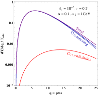
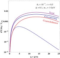
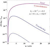
For completeness, we can include the contribution in Eq. (38), then this result also applies to the case if cuts through both and . Fig. 3 shows the differential DM density as a function of the comoving momentum in different phases, all calculated from Eq. (38) including all contributions. We will use this formula for numerical calculations of DM densities in the next section in all phases.
V Numerical results
In this section we present the numerical calculations of the dark matter relic abundance for various parameter choices of the model. We fix for the twin electromagnetic gauge coupling and calculate the DM density in units of the observed . All calculations are performed using Eq. (38) including contributions from all relevant processes.
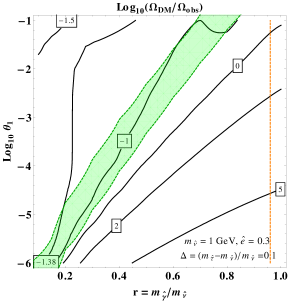
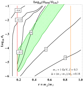
In Fig. 4, we consider GeV and plot the DM density dependence on and the mixing angle , for and . The contours are in and the “0” contour represents points which produce the observed DM density. The coscattering phase sits in the lower-right region, as for small and large the coscattering process is suppressed and freezes out earlier. The upper-left region, on the other hand, belongs to the coannihilation phase. The green band separating them corresponds to the mixed phase. The boundaries of the green band are determined by the condition and . The contribution to the relic density from modes with is small and is ignored in the coscattering calculation. The orange vertical dashed line corresponds to . To the right of it becomes relevant and we enter the mixed phase. The DM relic density is slightly reduced by compared to a pure coscattering calculation. The red vertical dashed line indicates . To the left of it the on-shell decay and inverse decay are open so this whole region is in the coannihilation phase.
The relic density in the coannhilation phase is mostly independent of because it is mainly controlled by which hardly depends on . Only at larger values when and become relevant the DM relic density shows some dependence. The dependence on of the relic density in the coannihilation phase is also mild, as it mainly affects the phase space of the coannihilation process. In the coscattering phase, the DM relic density increases as increases, which can be seen by comparing the two plots in Fig. 4. This is because a larger gap between and requires a higher threshold momentum for to make happen. Therefore the coscattering is suppressed, resulting in a larger relic density. For GeV, , the observed DM density is produced in the coscattering phase, while for it moves to the mixed phase or coannihilation phase.
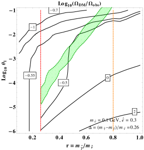
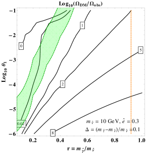
In Figs. 5 and 6 we show the results for MeV and 10 GeV. A larger DM mass will give a larger relic density if all other parameters are fixed. Consequently for a correct relic density we need a smaller (larger) for a larger (smaller) . The values are chosen to be 0.2 and 0.26 for the two plots with MeV, and 0.04 and 0.1 for the two plots with GeV. The behaviors of the contours are similar to the case of GeV.


VI Experimental Constraints and Tests
In this section we discuss the current experimental constraints and future experimental tests of this model. A comprehensive summary for this type of DM scenarios can be found in Ref. DAgnolo:2018wcn .
VI.1 Direct Detection
The dark matter interacts with SM particles through the Higgs portal or dark photon portal. The Higgs portal is suppressed by the Higgs mixing between the SM and twin sectors, and the twin neutrino Yukawa coupling. The dark photon portal is suppressed by the kinetic mixing , and also the mixing angle . Most current DM direct detection experiments are based on heavy nuclei recoiling when the nuclei scatter with the DM particles. They become ineffective for light DM less than a few GeV, but could potentially constrain the parameter space of heavier twin neutrino region, as the Yukawa coupling also becomes larger for a heavier twin neutrino. For =10 GeV and , the -nucleon cross section is of cm2, which is dominated by the Higgs portal. Such DM is not yet constrained by recent liquid xenon DM detectors daSilva:2017swg ; Aprile:2017iyp ; Cui:2017nnn . A conservative estimate according to Ref. Djouadi:2011aa gives an upper limit of 22(60) GeV on for .
For even lighter DM, recent upgrades/proposals of detecting DM-electron scattering can largely increase the sensitivity for sub-GeV mass DM Essig:2013lka ; Alexander:2016aln . In our model, the - couplings from both the dark photon portal and the Higgs portal are highly suppressed. The elastic cross section of scattering from the dark photon portal is
| (40) | |||||
where the reference values of mixing parameters , have been chosen close to the upper bounds to maximize the cross section. This is not yet constrained by recent electron-scattering experiments, including SENSEI Crisler:2018gci , Xenon10 Essig:2012yx , DarkSide-50 Agnes:2018oej . Future upgrades will be able to probe part of the parameter space with large mixings.
It is also worth mentioning that there are also crystal experiments based on phonon signals coming from DM scattering off nuclei in the detector, such as CRESST-III Petricca:2017zdp . Thanks to the low energy threshold ((50 eV)), these experiments will also be sensitive to the sub-GeV DM mass region. For such low DM mass, the dark photon portal becomes important and can dominate over the Higgs portal interaction if the mixings are not too small. However, the current constraint still can not put any bounds on even for the =3 case. Significant progress in the future could be helpful to constrain the parameter space for a light .
VI.2 Indirect Constraints Induced from DM Annihilation
Light DM is in general strongly constrained by indirect searches due to its high number density. WIMP models with annihilation cross section and GeV have already been ruled out Ade:2015xua . In our model the DM relic density is not determined by the DM annihilation process, but by the coannihilation and coscattering processes. The DM annihilation is dominated by , which is suppressed by . An upper bound on the DM annihilation cross section gives a constraint on the combination of the parameters . Fermi-LAT data Geringer-Sameth:2014qqa has put an upper limit on the DM annihilation cross section for DM heavier than 6 GeV. A stronger constraint comes from CMB observables, which restrict the net energy deposited from DM annihilation into visible particles during the reionization era Liu:2016cnk . The constraints from the Fermi-LAT and the Planck data are plotted in Fig. 7.
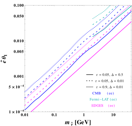
Note that the annihilation of can produce instead of . This may modify the bounds derived from the final state. The total energy injection is the same, and the final state will result in more electrons but with lower energies. Ref. Elor:2015bho performed a detailed study in comparing the constrains for cascade decays with different numbers of final sate particles. After convoluting with the energy dependence of the efficiency factor Slatyer:2015jla , it is found that the effects due to multi-step decay is rather mild. The constraints on the and final states from the Planck data are roughly the same. On the other hand, a higher-step cascade tends to soften the spectrum and thus slightly weakens the constraint from the Fermi-LAT result Elor:2015bho . The proposed ground-based CMB Stage-4 experiment Abazajian:2016yjj is expected to improve the constraint by a factor of 2 to 3 compared to Planck. The DM annihilation after the CMB era will also heat the intergalactic hydrogen gas and erase the absorption features of 21cm spectrum around . The recent measurement by the EDGES experiment instead observed an even stronger absorption than the standard astrophysical expectation Bowman:2018yin . If one interprets this result as a constraint that the DM annihilation should not significantly reduce the absorption, the observed brightness temperature then suggests an even stronger bound than the one from CMB DAmico:2018sxd ; Cheung:2018vww ; Berlin:2018sjs ; Barkana:2018qrx . In Fig. 7 we also plot the most conservative constraint in terms of according to Ref. DAmico:2018sxd , taking the efficiency factor to be 1. For GeV, the upper limit for is between and depending on other model parameters.222 The annihilation cross section depends on the model parameters as For a fixed mixing angle, the annihilation rate reaches its maximum around for very small , while for larger , it decreases as increases. The constraint gets more stringent for lighter .
VI.3 Constraints induced by the Light Twin Photon
In our scenario is the lightest twin sector particle. An on-shell decays through its kinetic mixing with the SM photon and there is no invisible decay mode to the twin sector. In this case, it is well described by two parameters: the twin photon mass and the kinematic mixing with the SM photon . Experimental constraints on dark photon have been extensively studied. Summeries of current status can be found in Refs. Curtin:2013fra ; Curtin:2014cca ; Alexander:2016aln ; Ilten:2018crw .
A lower bound on comes from the effective number of neutrinos () Boehm:2013jpa . A light can stay in thermal equilibrium with photons and electrons after the neutrinos decouple at MeV. The entropy transferred from to the photon bath will change the neutrino-photon temperature ratio, and therefore modify . Using the results in Ref. Boehm:2013jpa and the Planck data Ade:2015xua , we obtain a lower bound on around MeV. It may be further improved to MeV by the future CMB-S4 experiment Abazajian:2016yjj .
There are also many constraints on depending on . The current upper bounds for mostly come from colliders, fixed target experiments and meson decay experiments, in searching for prompt decay products. (See Ref. Ilten:2018crw for a summary and an extended reference list.) These experiments constrain in the mass range that we consider (except for a few narrow gaps at the meson resonances). The lower bounds for come from displaced decays from various beam dump experiments Bjorken:2009mm ; Bergsma:1985is ; Konaka:1986cb ; Riordan:1987aw ; Bjorken:1988as ; Bross:1989mp ; Davier:1989wz ; Athanassopoulos:1997er ; Astier:2001ck ; Essig:2010gu ; Williams:2011qb ; Blumlein:2011mv ; Gninenko:2012eq ; Blumlein:2013cua , and also from supernova SN1987A Chang:2016ntp . The Big Bang Nucleosynthesis (BBN) would also constrain the lifetime of . However, the decay of is only suppressed by and the BBN does not introduce extra constraints for Chang:2016ntp , which is required in this model to keep the DM sector in thermal contact with the SM. These bounds are summarized in Fig. 8.

VI.4 Constraints Induced from decay
As we require , the twin photon only decays to SM particles, thus can only be pair produced in a lab via an off-shell twin photon or from the Higgs boson decay. The constraints from pair production from off-shell are weaker compared to the ones from visible decay modes described in the previous subsection. Moreover, pair production via will be further suppressed by , leaving to be the main production channel.
At the LHC, the produced from / will be long-lived in general, if the two-body decay is forbidden (), because the leading three-body decay is suppressed by . Assuming and are Dirac fermions and taking , the current upper bound of the Higgs invisible decay branching ratio, Br( invisible) Khachatryan:2016vau ; Khachatryan:2016whc , constrains to be GeV for . HL-LHC is expected to improve the Higgs invisible branching ratio measurement to 6-8% Dawson:2013bba , which would translate to a bound GeV for . Future colliders can probe BR( invisible) to the sub-percent level Gomez-Ceballos:2013zzn ; Fujii:2015jha ; CEPC-SPPCStudyGroup:2015csa ; Abramowicz:2016zbo . A 0.3% measurement can constrain down to GeV for .
The decay width can be expressed analytically in the small limit ():
| (41) |
which strongly depends on and . Numerically the proper decay length is given by
| (42) |
where is the number of SM fermions that can appear in the final state. The dark sector could be probed by searching for displaced decays at the HL-LHC for (1) m Curtin:2017izq . Longer decay lengths may be tested at future proposed experiments, such as SHiP Alekhin:2015byh , MATHUSLA Curtin:2017izq , CODEX-b Gligorov:2017nwh , and FASER Feng:2017uoz .
If (1) second, the decays of thermal relic will inject energy during the BBN era and the recombination era. However, the constraint is weakened by the fact that only makes up a small fraction of after it freezes out (), also the fact that only a small fraction of energy would be injected. The strongest bound comes from the electromagnetic decay products and depends on the model parameters. Typically, the lifetime of the long-lived is only constrained by BBN to be shorter than seconds Poulin:2016anj ; Kawasaki:2017bqm . The extra energy injection from decays could distort the CMB blackbody spectrum which can potentially be captured by the proposed PIXIE mission Kogut:2011xw . It may give a slightly stronger bound than BBN on Poulin:2016anj , also around sec for our typical benchmark models.
In Fig 8, we also plot several benchmark points with fixed , , and , that give rise to the correct DM relic density from our numerical results in Sec. V. The vertical parts indicates that the thermal relic density is mostly independent of the gauge kinematic mixing parameter , as long as it can keep the DM in thermal equilibrium with SM before freeze-out. For large values of , the three-body (inverse) decay rate gets larger, and can even freeze out later than the coannihilation process . It drives the benchmark models to the coannihilation phase even if it was in the coscattering or mixed phase for smaller values of . This occurs for all our benchmark models except for model 5 (red line) which is in the coannihilation phase for all . The transition to the coannihilation phase reduces the DM number density, hence it needs a larger DM mass to compensate the effect. This explains the turn of the curves at lager values. However, except for model 2 (orange line), the turns occur in the region which has been ruled out by other experiments. For smaller , the lifetime becomes longer, which is constrained by the BBN bound. The region that violates the BBN constraint is indicated by dashed lines.
VII Conclusions
The necessity of DM in the universe is one of the strongest evidences of new physics beyond the SM. Experimental searches in various fronts so far have not revealed the nature of the DM. For the most popular WIMP DM scenario, recent advancements in experiments have covered significant fractions of the allowed parameter space, even though there are still viable parameter space left. People have taken more seriously the possibility that DM resides in a more hidden sector, and hence has escaped our intensive experimental searches. Even in this case, it would be more satisfactory if it is part of a bigger story, rather than just arises in an isolated sector for no particular reason. In this paper, we consider DM coming from a particle in the twin sector of the fraternal twin Higgs model, which itself is motivated by the naturalness problem of the SM EW symmetry breaking and non-discovery of the colored top partners at the colliders. Although the relevant particles for the DM relic density in our study, i.e., the twin neutrino, twin tau, and twin photon, have little effect on the naturalness of the EW scale, they are an integral part of the full theory that solves the naturalness problem, just like the neutralinos in a supersymmetric SM.
To obtain the correct DM relic density, the interplay of the twin neutrino, twin tau, and twin photon is important. The DM relic density is determined by the order of the freeze-out temperatures of various annihilation and scattering processes. It is in the coannihilation phase if the twin tau annihilation freezes out earlier than the twin neutrino to twin tau scattering. In the opposite limit, it realizes the recently discovered coscattering phase. There is also an intermediate regime where the DM relic density is determined by both coannihilation and coscattering processes due to the momentum dependence of the coscattering process. The calculation of the DM relic density in this mixed phase is more complicated and has not been done in the literature and we provide a reasonably simple way to evaluate it with very good accuracies.
There are many experimental constraints but none of them can cover the whole parameter space. Direct detection with nuclei recoiling can only constrain heavier DM, above a few GeV. The experiments based on electron scattering are not yet sensitive to this model. Future upgrades may be able to probe the region of the parameter space with large mixings between the twin tau and the twin neutrino. Indirect constraints from DM annihilation are more sensitive to smaller DM mass with large enough twin tau – twin neutrino mixings. Other constraints rely on the coannihilation/coscattering partners of the DM. Twin photon is subject to various dark photon constraints. Twin tau typically has a long lifetime so it is constrained by BBN and CMB. Its displaced decays may be searched at colliders with dedicated detectors or strategies. A big chunk of the parameter space still survives all the constraints. A complete coverage of the parameter space directly is not easy in the foreseeable future. An indirect test may come from the test of the whole fraternal twin Higgs model at a future high energy collider, if other heavier particles in the model can be produced.
acknowledgments
We would like to thank Zackaria Chacko, Rafael Lang, Natalia Toro, Yuhsin Tsai, and Po-Jen Wang for useful discussions. This work is supported in part by the US Department of Energy grant DE-SC-000999. H.-C. C. was also supported by The Ambrose Monell Foundation at the Institute for Advanced Study, Princeton.
Appendix A Calculation of the Collision Operator
The evaluation of the reduced collision operator can be time consuming to achieve a high precision. It can be simplified by performing a partial analytic integration of the phase space, leaving a one-dimensional integral for the numerical calculation. A similar treatment for a case with a massless initial state was done in Ref. Garny:2017rxs . Notice that since and the final state integrated in Eq. (33) are Lorentz invariant, can be evaluated in the rest frame of . The initial state momentum in the rest frame is a function of both and , obtained from a simple boost. In this frame, the density distribution of is no longer spherically symmetric, but is still axially symmetric along the boost axis. In addition, the Mandelstam variable is a function of only, so the integration over the angular variables can be easily performed and the result is
| (43) |
where = is the threshold momentum of for the upward scattering.
Appendix B The Effect of the (Inverse) Decay
When the decay and the inverse decay [] are kinematically allowed, the effect can also be included in the collision operator by an extra term . The cross section of the inverse decay takes the form:
| (44) |
where the flux . The unintegrated Boltzmann equation (31) now reads
| (45) |
with the inverse decay contribution given by
| (46) | ||||
| (47) | ||||
| (48) |
where
| (49) |
Notice that the kinematic threshold of the inverse decay is lower than that of the coscattering because it does not need to create a twin photon in the final state. For example, the ratio of the threshold momenta for is
| (50) |
which is larger than one for any and . The interaction rate of is hence exponentially suppressed compared to the rate of , besides that it has an extra suppression. Consequently decouples much later than .
To compare the decoupling time between the inverse decay and the coannihilation , we can simply compare with when decouples. For , is simplified to:
We find that in the parameter space that we consider with , the (inverse) decay is still active when decouples. As an example, for , GeV, decouples at , much later than that decouples at . The difference is even larger for lower values of and . From these comparisons, we conclude that when , the (inverse) decay will keep and in chemical equilibrium and makes the relic density follow the coannihilation result.
Appendix C The Relic Density Calculation from Iteration
As the coscattering process freezes out, the assumption of chemical equilibrium between and (Eq. (26)) breaks down. As a result, the combined Boltzmann equation for and Eq. (27) no longer holds after freezes out. In the mixed phase when and are comparable, in principle one should solve the coupled Boltzmann equations for both and . As the distribution of remains canonical due to scattering, we can integrate out the momentum dependence to obtain the integrated Boltzmann equation for ,
| (51) |
where the last term is the contribution from the inverse coscattering process , which does not have a threshold and has very weak dependence. The combination of Eq. (51) and Eq. (38) will give the full solution of and .
One way to solve the coupled equations is to use the iterative method Garny:2017rxs . With an initial guess of , we can obtain from solving Eq. (51). Plugging it into Eq. (38) will return an improved value for . Repeating this process will eventually converges to the exact result.

We take the number densities obtained from the coannihilation calculation as our starting point. We argued that in this case Eq. (38) gives the correct results both in the coannihilation limit and the coscattering limit without iterations. The only possibility of significant deviation is when their contributions are comparable, i.e., in the mixed phase. To examine the corrections from iterations, we perform numerical studies for the benchmark parameters, GeV, , and , with , which correspond to coannihilation, mixed, and coscattering phases respectively. We found that the correction of from a single iteration is always small. The results are shown in Fig. 9. The first plot represents a coannihilation-like phase. The correction due to the coscattering contribution from the first iteration is less than . For smaller the coscattering becomes more important one can see larger deviations in , due to the larger from decoupling of . In the coscattering phase as shown in the bottom plot, the correction of at late time can be significant. However, during freeze-out (which occurs at for ), is still approximately in equilibrium, and the relic density is mostly given by . The correction to the total DM density is also small ( in this case). The largest correction from the iteration indeed happens in the mixed phase, although it is still quite small. For , the correction to is from the first iteration. The reason for such small corrections is that is not as sensitive to the early decoupling as is, therefore using from the coannihilation calculation in Eq. (38) gives a very good approximation. Based on these results, in our numerical calculations we simply adopt this prescription without iterations.
References
- (1) Z. Chacko, H. S. Goh and R. Harnik, “The Twin Higgs: Natural electroweak breaking from mirror symmetry,” Phys. Rev. Lett. 96, 231802 (2006) doi:10.1103/PhysRevLett.96.231802 [hep-ph/0506256].
- (2) N. Craig, A. Katz, M. Strassler and R. Sundrum, “Naturalness in the Dark at the LHC,” JHEP 1507, 105 (2015) doi:10.1007/JHEP07(2015)105 [arXiv:1501.05310 [hep-ph]].
- (3) I. Garcia Garcia, R. Lasenby and J. March-Russell, “Twin Higgs WIMP Dark Matter,” Phys. Rev. D 92, no. 5, 055034 (2015) doi:10.1103/PhysRevD.92.055034 [arXiv:1505.07109 [hep-ph]].
- (4) N. Craig and A. Katz, “The Fraternal WIMP Miracle,” JCAP 1510, no. 10, 054 (2015) doi:10.1088/1475-7516/2015/10/054 [arXiv:1505.07113 [hep-ph]].
- (5) I. Garcia Garcia, R. Lasenby and J. March-Russell, “Twin Higgs Asymmetric Dark Matter,” Phys. Rev. Lett. 115, no. 12, 121801 (2015) doi:10.1103/PhysRevLett.115.121801 [arXiv:1505.07410 [hep-ph]].
- (6) M. Farina, “Asymmetric Twin Dark Matter,” JCAP 1511, no. 11, 017 (2015) doi:10.1088/1475-7516/2015/11/017 [arXiv:1506.03520 [hep-ph]].
- (7) R. T. D’Agnolo, D. Pappadopulo and J. T. Ruderman, “Fourth Exception in the Calculation of Relic Abundances,” Phys. Rev. Lett. 119, no. 6, 061102 (2017) doi:10.1103/PhysRevLett.119.061102 [arXiv:1705.08450 [hep-ph]].
- (8) M. Garny, J. Heisig, B. Lülf and S. Vogl, “Coannihilation without chemical equilibrium,” Phys. Rev. D 96, no. 10, 103521 (2017) doi:10.1103/PhysRevD.96.103521 [arXiv:1705.09292 [hep-ph]].
- (9) K. Griest and D. Seckel, “Three exceptions in the calculation of relic abundances,” Phys. Rev. D 43, 3191 (1991). doi:10.1103/PhysRevD.43.3191
- (10) G. Bélanger, F. Boudjema, A. Goudelis, A. Pukhov and B. Zaldivar, “micrOMEGAs5.0 : freeze-in,” arXiv:1801.03509 [hep-ph].
- (11) T. Bringmann, J. Edsjö, P. Gondolo, P. Ullio and L. Bergström, “DarkSUSY 6 : An Advanced Tool to Compute Dark Matter Properties Numerically,” arXiv:1802.03399 [hep-ph].
- (12) F. Ambrogi, C. Arina, M. Backovic, J. Heisig, F. Maltoni, L. Mantani, O. Mattelaer and G. Mohlabeng, “MadDM v.3.0: a Comprehensive Tool for Dark Matter Studies,” arXiv:1804.00044 [hep-ph].
- (13) Z. Chacko, N. Craig, P. J. Fox and R. Harnik, “Cosmology in Mirror Twin Higgs and Neutrino Masses,” JHEP 1707, 023 (2017) doi:10.1007/JHEP07(2017)023 [arXiv:1611.07975 [hep-ph]].
- (14) N. Craig, S. Koren and T. Trott, “Cosmological Signals of a Mirror Twin Higgs,” JHEP 1705, 038 (2017) doi:10.1007/JHEP05(2017)038 [arXiv:1611.07977 [hep-ph]].
- (15) R. Barbieri, L. J. Hall and K. Harigaya, “Minimal Mirror Twin Higgs,” JHEP 1611, 172 (2016) doi:10.1007/JHEP11(2016)172 [arXiv:1609.05589 [hep-ph]].
- (16) C. Csaki, E. Kuflik and S. Lombardo, “Viable Twin Cosmology from Neutrino Mixing,” Phys. Rev. D 96, no. 5, 055013 (2017) doi:10.1103/PhysRevD.96.055013 [arXiv:1703.06884 [hep-ph]].
- (17) R. Barbieri, L. J. Hall and K. Harigaya, “Effective Theory of Flavor for Minimal Mirror Twin Higgs,” JHEP 1710, 015 (2017) doi:10.1007/JHEP10(2017)015 [arXiv:1706.05548 [hep-ph]].
- (18) S. Mizuta and M. Yamaguchi, “Coannihilation effects and relic abundance of Higgsino dominant LSP(s),” Phys. Lett. B 298, 120 (1993) doi:10.1016/0370-2693(93)91717-2 [hep-ph/9208251].
- (19) R. T. D’Agnolo, C. Mondino, J. T. Ruderman and P. J. Wang, “Exponentially Light Dark Matter from Coannihilation,” arXiv:1803.02901 [hep-ph].
- (20) C. F. P. da Silva [LUX Collaboration], “Dark Matter Searches with LUX,” arXiv:1710.03572 [hep-ex].
- (21) E. Aprile et al. [XENON Collaboration], “First Dark Matter Search Results from the XENON1T Experiment,” Phys. Rev. Lett. 119, no. 18, 181301 (2017) doi:10.1103/PhysRevLett.119.181301 [arXiv:1705.06655 [astro-ph.CO]], and new results which can be found at http://www.xenon1t.org.
- (22) X. Cui et al. [PandaX-II Collaboration], “Dark Matter Results From 54-Ton-Day Exposure of PandaX-II Experiment,” Phys. Rev. Lett. 119, no. 18, 181302 (2017) doi:10.1103/PhysRevLett.119.181302 [arXiv:1708.06917 [astro-ph.CO]].
- (23) A. Djouadi, O. Lebedev, Y. Mambrini and J. Quevillon, “Implications of LHC searches for Higgs–portal dark matter,” Phys. Lett. B 709, 65 (2012) doi:10.1016/j.physletb.2012.01.062 [arXiv:1112.3299 [hep-ph]].
- (24) R. Essig et al., “Working Group Report: New Light Weakly Coupled Particles,” arXiv:1311.0029 [hep-ph].
- (25) J. Alexander et al., “Dark Sectors 2016 Workshop: Community Report,” arXiv:1608.08632 [hep-ph].
- (26) M. Crisler et al. [SENSEI Collaboration], “SENSEI: First Direct-Detection Constraints on sub-GeV Dark Matter from a Surface Run,” arXiv:1804.00088 [hep-ex].
- (27) R. Essig, A. Manalaysay, J. Mardon, P. Sorensen and T. Volansky, “First Direct Detection Limits on sub-GeV Dark Matter from XENON10,” Phys. Rev. Lett. 109, 021301 (2012) doi:10.1103/PhysRevLett.109.021301 [arXiv:1206.2644 [astro-ph.CO]].
- (28) P. Agnes et al. [DarkSide Collaboration], “Constraints on Sub-GeV Dark Matter-Electron Scattering from the DarkSide-50 Experiment,” arXiv:1802.06998 [astro-ph.CO].
- (29) F. Petricca et al. [CRESST Collaboration], arXiv:1711.07692 [astro-ph.CO].
- (30) P. A. R. Ade et al. [Planck Collaboration], “Planck 2015 results. XIII. Cosmological parameters,” Astron. Astrophys. 594, A13 (2016) doi:10.1051/0004-6361/201525830 [arXiv:1502.01589 [astro-ph.CO]].
- (31) A. Geringer-Sameth, S. M. Koushiappas and M. G. Walker, “Comprehensive search for dark matter annihilation in dwarf galaxies,” Phys. Rev. D 91, no. 8, 083535 (2015) doi:10.1103/PhysRevD.91.083535 [arXiv:1410.2242 [astro-ph.CO]].
- (32) H. Liu, T. R. Slatyer and J. Zavala, “Contributions to cosmic reionization from dark matter annihilation and decay,” Phys. Rev. D 94, no. 6, 063507 (2016) doi:10.1103/PhysRevD.94.063507 [arXiv:1604.02457 [astro-ph.CO]].
- (33) G. Elor, N. L. Rodd, T. R. Slatyer and W. Xue, JCAP 1606, no. 06, 024 (2016) doi:10.1088/1475-7516/2016/06/024 [arXiv:1511.08787 [hep-ph]].
- (34) T. R. Slatyer, Phys. Rev. D 93, no. 2, 023527 (2016) doi:10.1103/PhysRevD.93.023527 [arXiv:1506.03811 [hep-ph]].
- (35) K. N. Abazajian et al. [CMB-S4 Collaboration], “CMB-S4 Science Book, First Edition,” arXiv:1610.02743 [astro-ph.CO].
- (36) J. D. Bowman, A. E. E. Rogers, R. A. Monsalve, T. J. Mozdzen and N. Mahesh, “An absorption profile centred at 78 megahertz in the sky-averaged spectrum,” Nature 555, no. 7694, 67 (2018). doi:10.1038/nature25792
- (37) G. D’Amico, P. Panci and A. Strumia, “Bounds on Dark Matter annihilations from 21 cm data,” arXiv:1803.03629 [astro-ph.CO].
- (38) K. Cheung, J. L. Kuo, K. W. Ng and Y. L. S. Tsai, “The impact of EDGES 21-cm data on dark matter interactions,” arXiv:1803.09398 [astro-ph.CO].
- (39) R. Barkana, N. J. Outmezguine, D. Redigolo and T. Volansky, “Signs of Dark Matter at 21-cm?,” arXiv:1803.03091 [hep-ph].
- (40) A. Berlin, D. Hooper, G. Krnjaic and S. D. McDermott, “Severely Constraining Dark Matter Interpretations of the 21-cm Anomaly,” arXiv:1803.02804 [hep-ph].
- (41) D. Curtin et al., “Exotic decays of the 125 GeV Higgs boson,” Phys. Rev. D 90, no. 7, 075004 (2014) doi:10.1103/PhysRevD.90.075004 [arXiv:1312.4992 [hep-ph]].
- (42) D. Curtin, R. Essig, S. Gori and J. Shelton, “Illuminating Dark Photons with High-Energy Colliders,” JHEP 1502, 157 (2015) doi:10.1007/JHEP02(2015)157 [arXiv:1412.0018 [hep-ph]].
- (43) P. Ilten, Y. Soreq, M. Williams and W. Xue, “Serendipity in dark photon searches,” arXiv:1801.04847 [hep-ph].
- (44) C. Boehm, M. J. Dolan and C. McCabe, “A Lower Bound on the Mass of Cold Thermal Dark Matter from Planck,” JCAP 1308, 041 (2013) doi:10.1088/1475-7516/2013/08/041 [arXiv:1303.6270 [hep-ph]].
- (45) J. D. Bjorken, R. Essig, P. Schuster and N. Toro, “New Fixed-Target Experiments to Search for Dark Gauge Forces,” Phys. Rev. D 80, 075018 (2009) doi:10.1103/PhysRevD.80.075018 [arXiv:0906.0580 [hep-ph]].
- (46) F. Bergsma et al. [CHARM Collaboration], “A Search for Decays of Heavy Neutrinos in the Mass Range 0.5-GeV to 2.8-GeV,” Phys. Lett. 166B, 473 (1986). doi:10.1016/0370-2693(86)91601-1
- (47) A. Konaka et al., “Search for Neutral Particles in Electron Beam Dump Experiment,” Phys. Rev. Lett. 57, 659 (1986). doi:10.1103/PhysRevLett.57.659
- (48) E. M. Riordan et al., “A Search for Short Lived Axions in an Electron Beam Dump Experiment,” Phys. Rev. Lett. 59, 755 (1987). doi:10.1103/PhysRevLett.59.755
- (49) J. D. Bjorken et al., “Search for Neutral Metastable Penetrating Particles Produced in the SLAC Beam Dump,” Phys. Rev. D 38, 3375 (1988). doi:10.1103/PhysRevD.38.3375
- (50) A. Bross, M. Crisler, S. H. Pordes, J. Volk, S. Errede and J. Wrbanek, “A Search for Shortlived Particles Produced in an Electron Beam Dump,” Phys. Rev. Lett. 67, 2942 (1991). doi:10.1103/PhysRevLett.67.2942
- (51) M. Davier and H. Nguyen Ngoc, “An Unambiguous Search for a Light Higgs Boson,” Phys. Lett. B 229, 150 (1989). doi:10.1016/0370-2693(89)90174-3
- (52) C. Athanassopoulos et al. [LSND Collaboration], “Evidence for muon-neutrino —¿ electron-neutrino oscillations from pion decay in flight neutrinos,” Phys. Rev. C 58, 2489 (1998) doi:10.1103/PhysRevC.58.2489 [nucl-ex/9706006].
- (53) P. Astier et al. [NOMAD Collaboration], “Search for heavy neutrinos mixing with tau neutrinos,” Phys. Lett. B 506, 27 (2001) doi:10.1016/S0370-2693(01)00362-8 [hep-ex/0101041].
- (54) R. Essig, R. Harnik, J. Kaplan and N. Toro, “Discovering New Light States at Neutrino Experiments,” Phys. Rev. D 82, 113008 (2010) doi:10.1103/PhysRevD.82.113008 [arXiv:1008.0636 [hep-ph]].
- (55) M. Williams, C. P. Burgess, A. Maharana and F. Quevedo, “New Constraints (and Motivations) for Abelian Gauge Bosons in the MeV-TeV Mass Range,” JHEP 1108, 106 (2011) doi:10.1007/JHEP08(2011)106 [arXiv:1103.4556 [hep-ph]].
- (56) J. Blumlein and J. Brunner, “New Exclusion Limits for Dark Gauge Forces from Beam-Dump Data,” Phys. Lett. B 701, 155 (2011) doi:10.1016/j.physletb.2011.05.046 [arXiv:1104.2747 [hep-ex]].
- (57) S. N. Gninenko, “Constraints on sub-GeV hidden sector gauge bosons from a search for heavy neutrino decays,” Phys. Lett. B 713, 244 (2012) doi:10.1016/j.physletb.2012.06.002 [arXiv:1204.3583 [hep-ph]].
- (58) J. Blümlein and J. Brunner, “New Exclusion Limits on Dark Gauge Forces from Proton Bremsstrahlung in Beam-Dump Data,” Phys. Lett. B 731, 320 (2014) doi:10.1016/j.physletb.2014.02.029 [arXiv:1311.3870 [hep-ph]].
- (59) J. H. Chang, R. Essig and S. D. McDermott, “Revisiting Supernova 1987A Constraints on Dark Photons,” JHEP 1701, 107 (2017) doi:10.1007/JHEP01(2017)107 [arXiv:1611.03864 [hep-ph]].
- (60) G. Aad et al. [ATLAS and CMS Collaborations], “Measurements of the Higgs boson production and decay rates and constraints on its couplings from a combined ATLAS and CMS analysis of the LHC pp collision data at and 8 TeV,” JHEP 1608, 045 (2016) doi:10.1007/JHEP08(2016)045 [arXiv:1606.02266 [hep-ex]].
- (61) V. Khachatryan et al. [CMS Collaboration], “Searches for invisible decays of the Higgs boson in pp collisions at = 7, 8, and 13 TeV,” JHEP 1702, 135 (2017) doi:10.1007/JHEP02(2017)135 [arXiv:1610.09218 [hep-ex]].
- (62) S. Dawson et al., “Working Group Report: Higgs Boson,” arXiv:1310.8361 [hep-ex].
- (63) M. Bicer et al. [TLEP Design Study Working Group], “First Look at the Physics Case of TLEP,” JHEP 1401, 164 (2014) doi:10.1007/JHEP01(2014)164 [arXiv:1308.6176 [hep-ex]].
- (64) K. Fujii et al., “Physics Case for the International Linear Collider,” arXiv:1506.05992 [hep-ex].
- (65) CEPC-SPPC Study Group, “CEPC-SPPC Preliminary Conceptual Design Report. 1. Physics and Detector,” IHEP-CEPC-DR-2015-01, IHEP-TH-2015-01, IHEP-EP-2015-01.
- (66) H. Abramowicz et al., “Higgs physics at the CLIC electron?positron linear collider,” Eur. Phys. J. C 77, no. 7, 475 (2017) doi:10.1140/epjc/s10052-017-4968-5 [arXiv:1608.07538 [hep-ex]].
- (67) D. Curtin and M. E. Peskin, “Analysis of Long Lived Particle Decays with the MATHUSLA Detector,” Phys. Rev. D 97, no. 1, 015006 (2018) doi:10.1103/PhysRevD.97.015006 [arXiv:1705.06327 [hep-ph]].
- (68) S. Alekhin et al., “A facility to Search for Hidden Particles at the CERN SPS: the SHiP physics case,” Rept. Prog. Phys. 79, no. 12, 124201 (2016) doi:10.1088/0034-4885/79/12/124201 [arXiv:1504.04855 [hep-ph]].
- (69) V. V. Gligorov, S. Knapen, M. Papucci and D. J. Robinson, “Searching for Long-lived Particles: A Compact Detector for Exotics at LHCb,” Phys. Rev. D 97, no. 1, 015023 (2018) doi:10.1103/PhysRevD.97.015023 [arXiv:1708.09395 [hep-ph]].
- (70) J. Feng, I. Galon, F. Kling and S. Trojanowski, “ForwArd Search ExpeRiment at the LHC,” Phys. Rev. D 97, no. 3, 035001 (2018) doi:10.1103/PhysRevD.97.035001 [arXiv:1708.09389 [hep-ph]].
- (71) V. Poulin, J. Lesgourgues and P. D. Serpico, “Cosmological constraints on exotic injection of electromagnetic energy,” JCAP 1703, no. 03, 043 (2017) doi:10.1088/1475-7516/2017/03/043 [arXiv:1610.10051 [astro-ph.CO]].
- (72) M. Kawasaki, K. Kohri, T. Moroi and Y. Takaesu, “Revisiting Big-Bang Nucleosynthesis Constraints on Long-Lived Decaying Particles,” Phys. Rev. D 97, no. 2, 023502 (2018) doi:10.1103/PhysRevD.97.023502 [arXiv:1709.01211 [hep-ph]].
- (73) A. Kogut et al., “The Primordial Inflation Explorer (PIXIE): A Nulling Polarimeter for Cosmic Microwave Background Observations,” JCAP 1107, 025 (2011) doi:10.1088/1475-7516/2011/07/025 [arXiv:1105.2044 [astro-ph.CO]].