On Consensus-Optimality Trade-offs in Collaborative Deep Learning

Zhanhong Jiang Department of Mechanical Engineering, Iowa State University Aditya Balu Department of Mechanical Engineering, Iowa State University Chinmay Hegde Department of Electrical and Computer Engineering, Iowa State University
{zhjiang|baditya|chinmay|soumiks}@iastate.edu
Soumik Sarkar Department of Mechanical Engineering, Iowa State University
Abstract

In distributed machine learning, where agents collaboratively learn from diverse private data sets, there is a fundamental tension between consensus and optimality. In this paper, we build on recent algorithmic progresses in distributed deep learning to explore various consensus-optimality trade-offs over a fixed communication topology. First, we propose the incremental consensus-based distributed SGD (i-CDSGD) algorithm, which involves multiple consensus steps (where each agent communicates information with its neighbors) within each SGD iteration. Second, we propose the generalized consensus-based distributed SGD (g-CDSGD) algorithm that enables us to navigate the full spectrum from complete consensus (all agents agree) to complete disagreement (each agent converges to individual model parameters). We analytically establish convergence of the proposed algorithms for strongly convex and nonconvex objective functions; we also analyze the momentum variants of the algorithms for the strongly convex case. We support our algorithms via numerical experiments, and demonstrate significant improvements over existing methods for collaborative deep learning.

1   Introduction

Scaling up deep learning algorithms in a distributed setting [1, 2, 3] is becoming increasingly critical, impacting several applications such as learning in robotic networks [4], the Internet of Things (IoT) [5, 6], and mobile device networks [7]. Several distributed deep learning approaches have been proposed to address issues such as model parallelism [8], data parallelism [8, 9], and the role of communication and computation [10, 11].

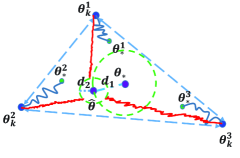
We focus on the constrained communication topology setting where the data is distributed (so that each agent has its own estimate of the deep model) and where information exchange among the learning agents are constrained along the edges of a given communication graph [9, 12]. In this context, two key aspects arise: consensus and optimality. We refer the reader to Figure 1 for an illustration involving 3 agents. With sufficient information exchange, the learned model parameters corresponding to each agent, θkj,j=1,2,3formulae-sequencesubscriptsuperscript𝜃𝑗𝑘𝑗123\theta^{j}_{k},j=1,2,3 could converge to θ^^𝜃\hat{\theta}, in which case they achieve consensus but not optimality (here, θsubscript𝜃\theta_{*} is the optimal model estimate if all the data were centralized). On the other hand, if no communication happens, the agents may approach their individual model estimates (θisubscriptsuperscript𝜃𝑖\theta^{i}_{*}) while being far from consensus. The question is whether this trade-off between consensus and optimality can be balanced so that all agents collectively agree upon a model estimate close to θsubscript𝜃\theta_{*}.

Our contributions: In this paper, we propose, analyze, and empirically evaluate two new algorithmic frameworks for distributed deep learning that enable us to explore fundamental trade-offs between consensus and optimality. The first approach is called incremental consensus-based distributed SGD (i-CDSGD), which is a stochastic extension of the descent-style algorithm proposed in [13]. This involves running multiple consensus steps where each agent exchanges information with its neighbors within each SGD iteration. The second approach is called generalized consensus-based distributed SGD (g-CDSGD), based on the concept of generalized gossip [14]. This involves a tuning parameter that explicitly controls the trade-off between consensus and optimality. Specifically, we:

  • (Algorithmic) propose the i-CDSGD and g-CDSGD algorithms (along with their momentum variants).

  • (Theoretical) prove the convergence of g-CDSGD (Theorems 1 & 3) and i-CDSGD (Theorems 2 & 4) for strongly convex and non-convex objective functions;

  • (Theoretical) prove the convergence of the momentum variants of g-CDSGD (Theorem 5) and i-CDSGD (Theorem 6) for strongly convex objective functions;

  • (Practical) empirically demonstrate that i-CDMSGD (the momentum variant of i-CDSGD) can achieve similar (global) accuracy as the state-of-the-art with lower fluctuation across epochs as well as better consensus;

  • (Practical) empirically demonstrate that g-CDMSGD (the momentum variant of g-CDSGD) can achieve similar (global) accuracy as the state-of-the-art with lower fluctuation, smaller generalization error and better consensus.

We use both balanced and unbalanced data sets (i.e., equal or unequal distributions of training samples among the agents) for the numerical experiments with benchmark deep learning data sets. Please see Table 1 for a detailed comparison with existing algorithms.

Method f𝑓f Con.Bou. Opt.Bou. Con.Rate Mom.Ana. C.C.T. Sto.
FedAvg [15] Nonconvex N/A N/A N/A No No Yes
DGDτ𝐷𝐺superscript𝐷𝜏DGD^{\tau} [13] Str-con 𝒪(α1λ2τ)𝒪𝛼1superscriptsubscript𝜆2𝜏\mathcal{O}(\frac{\alpha}{1-\lambda_{2}^{\tau}}) 𝒪(α1λ2τ)𝒪𝛼1superscriptsubscript𝜆2𝜏\mathcal{O}(\frac{\alpha}{1-\lambda_{2}^{\tau}}) 𝒪(ϵk)𝒪superscriptitalic-ϵ𝑘\mathcal{O}(\epsilon^{k}) No Yes No
MSDA [16] Str-con N/A N/A 𝒪(ϵk)𝒪superscriptitalic-ϵ𝑘\mathcal{O}(\epsilon^{k}) Yes Yes No
CDSGD [9] Str-con 𝒪(α1λ2)𝒪𝛼1subscript𝜆2\mathcal{O}(\frac{\alpha}{1-\lambda_{2}}) 𝒪(αγ+1H+α1(1λ2))𝒪𝛼𝛾1𝐻superscript𝛼11subscript𝜆2\mathcal{O}(\frac{\alpha\gamma+1}{H+\alpha^{-1}(1-\lambda_{2})}) 𝒪(ϵk)𝒪superscriptitalic-ϵ𝑘\mathcal{O}(\epsilon^{k}) No Yes Yes
Nonconvex 𝒪(α1λ2)𝒪𝛼1subscript𝜆2\mathcal{O}(\frac{\alpha}{1-\lambda_{2}}) 𝒪(αγ+1λN)𝒪𝛼𝛾1subscript𝜆𝑁\mathcal{O}(\alpha\gamma+1-\lambda_{N}) N/A
Acc-DNGD-SC [17] Str-con 𝒪(α13(1λ2)λ223)𝒪superscript𝛼131subscript𝜆2superscriptsubscript𝜆223\mathcal{O}(\frac{\alpha^{\frac{1}{3}}}{(1-\lambda_{2})\lambda_{2}^{\frac{2}{3}}}) N/A 𝒪(ϵk)𝒪superscriptitalic-ϵ𝑘\mathcal{O}(\epsilon^{k}) Yes Yes No
i-CDSGD [This paper] Str-con 𝒪(α1λ2τ)𝒪𝛼1superscriptsubscript𝜆2𝜏\mathcal{O}(\frac{\alpha}{1-\lambda_{2}^{\tau}}) 𝒪(αγ+1H+α1(1λ2τ))𝒪𝛼𝛾1𝐻superscript𝛼11superscriptsubscript𝜆2𝜏\mathcal{O}(\frac{\alpha\gamma+1}{H+\alpha^{-1}(1-\lambda_{2}^{\tau})}) 𝒪(ϵk)𝒪superscriptitalic-ϵ𝑘\mathcal{O}(\epsilon^{k}) Yes Yes Yes
Nonconvex 𝒪(α1λ2τ)𝒪𝛼1superscriptsubscript𝜆2𝜏\mathcal{O}(\frac{\alpha}{1-\lambda_{2}^{\tau}}) 𝒪(αγ+1λNτ)𝒪𝛼𝛾1superscriptsubscript𝜆𝑁𝜏\mathcal{O}(\alpha\gamma+1-\lambda_{N}^{\tau}) N/A
g-CDSGD [This paper] Str-con 𝒪(ωα1λ2)𝒪𝜔𝛼1subscript𝜆2\mathcal{O}(\frac{\omega\alpha}{1-\lambda_{2}}) 𝒪(αγ1+ω1H)𝒪𝛼𝛾1superscript𝜔1𝐻\mathcal{O}(\frac{\alpha\gamma-1+\omega^{-1}}{H}) 𝒪(ϵk)𝒪superscriptitalic-ϵ𝑘\mathcal{O}(\epsilon^{k}) Yes Yes Yes
Nonconvex 𝒪(ωα1λ2)𝒪𝜔𝛼1subscript𝜆2\mathcal{O}(\frac{\omega\alpha}{1-\lambda_{2}}) 𝒪(ωαγ+(1ω)(1λN))𝒪𝜔𝛼𝛾1𝜔1subscript𝜆𝑁\mathcal{O}(\omega\alpha\gamma+(1-\omega)(1-\lambda_{N})) N/A
  • Con.Bou.: consensus bound. Opt.Bou.: optimality bound. Con.Rate: convergence rate. Str-con: strongly convex. Mom.Ana.: momentum analysis. α𝛼\alpha: step size. λ2(0,1)subscript𝜆201\lambda_{2}\in(0,1): the second largest eigen-value of a stochastic matrix. τ𝜏\tau\in\mathbb{N}: positive constant. ω(0,1]𝜔01\omega\in(0,1]: a positive constant. ϵ(0,1)italic-ϵ01\epsilon\in(0,1): a positive constant, and it signifies the representative meaning. They are not exactly the same in different methods. Sto.: stochastic. C.C.T.: constrained communication topology. c1,c2>0subscript𝑐1subscript𝑐20c_{1},c_{2}\textgreater 0: condition numbers. H𝐻H: strong convexity constant. γ1,γ2,γ3>0subscript𝛾1subscript𝛾2subscript𝛾30\gamma_{1},\gamma_{2},\gamma_{3}\textgreater 0: smoothness constants.

Table 1: Comparisons between different optimization approaches

Related work: A large literature has emerged that studies distributed deep learning in both centralized and decentralized settings [8, 15, 18, 19, 3, 20, 21, 22], and due to space limitations we only summarize the most recent work. [23] propose a gradient sparsification approach for communication-efficient distributed learning, while  [24] propose the concept of ternary gradients to reduce communication costs. [16] propose a multi-step dual accelerated method using a gossip protocol to provide an optimal decentralized optimization algorithm for smooth and strongly convex loss functions. Decentralized parallel stochastic gradient descent [12] has also been proposed.

Perhaps most closely related to this paper is the work of [13], who present a distributed optimization method (called DGDτ𝐷𝐺superscript𝐷𝜏DGD^{\tau}) to enable consensus when the cost of communication is cheap. However, the authors only considered convex optimization problems, and only study deterministic gradient updates. Also, [17] propose a class of (deterministic) accelerated distributed Nesterov gradient descent methods to achieve linear convergence rate, for the special case of strongly convex objective functions. In [25], both deterministic and stochastic distributed were discussed while the algorithm had no acceleration techniques. To our knowledge, none of these previous works have explicitly studied the trade-off between consensus and optimality.
Refer to caption
Figure 1: A closer look at the optimization updates in distributed deep learning: Blue dots represent the current states (i.e., learned model parameters) of the agents; green dots represent the individual local optima (θisubscriptsuperscriptθi\theta^{i}_{*}), that agents converge to without sufficient consensus; the purple dot (θsubscriptθ\theta_{*}) represents the ideal optimal point for the entire agent population; another purple dot θ^^θ\hat{\theta} represents a possible consensus point for the agents which is far from optimal; blue and red curves signify the convergence trajectories with different step sizes; the green dashed circles indicate the neighborhoods of θsubscriptθ\theta_{*} and θ^^θ\hat{\theta}, respectively; d2subscriptd2d_{2} represents the consensus bound/error and d1subscriptd1d_{1} represents the optimality bound/error; ideally, both of these bounds should be small.

Outline: Section 2 presents the problem and several mathematical preliminaries. In Section 3, we present our two algorithmic frameworks, along with their analysis in Section 4. For validating the proposed schemes, several experimental results based on benchmark data sets are presented in Section 5. Concluding remarks are in Section 6.

2   Problem Formulation

We consider the standard unconstrained empirical risk minimization (ERM) problem typically used in machine learning problems (such as deep learning):

min1ni=1nfi(θ),min1𝑛superscriptsubscript𝑖1𝑛superscript𝑓𝑖𝜃\text{min}\,\frac{1}{n}\sum_{i=1}^{n}f^{i}(\theta), (1)

where θd𝜃superscript𝑑\theta\in\mathbb{R}^{d} denotes the parameter vector of interest, f:d:𝑓superscript𝑑f:\mathbb{R}^{d}\to\mathbb{R} denotes a given loss function, and fisuperscript𝑓𝑖f^{i} is the function value corresponding to a data point i𝑖i. Our focus is to investigate the case where the ERM problem is solved collaboratively among a number of computational agents. In this paper, we are interested in problems where the agents exhibit data parallelism, i.e., they only have access to their own respective training datasets. However, we assume that the agents can communicate over a static undirected graph 𝒢=(𝒱,)𝒢𝒱\mathcal{G}=(\mathcal{V},\mathcal{E}), where 𝒱𝒱\mathcal{V} is a vertex set (with nodes corresponding to agents) and \mathcal{E} is an edge set. Throughout this paper we assume that the graph 𝒢𝒢\mathcal{G} is connected.

Let 𝒟j,j=1,,nformulae-sequencesubscript𝒟𝑗𝑗1𝑛\mathcal{D}_{j},~{}j=1,\ldots,n denote the subset of the training data (comprising njsubscript𝑛𝑗n_{j} samples) corresponding to the jthsuperscript𝑗thj^{\textrm{th}} agent such that j=1Nnj=nsuperscriptsubscript𝑗1𝑁subscript𝑛𝑗𝑛\sum_{j=1}^{N}n_{j}=n, where N𝑁N is the total number of agents. With this formulation, and since f(θ)=j=1Nfj(θ)𝑓𝜃superscriptsubscript𝑗1𝑁subscript𝑓𝑗𝜃f(\theta)=\sum_{j=1}^{N}f_{j}(\theta), we have the following (constrained) reformulation of  (1):

minj=1Ni𝒟jfji(θj),s.t. θj=θl(j,l),minsuperscriptsubscript𝑗1𝑁subscript𝑖subscript𝒟𝑗subscriptsuperscript𝑓𝑖𝑗superscript𝜃𝑗s.t. superscript𝜃𝑗superscript𝜃𝑙for-all𝑗𝑙\text{min}\,\sum_{j=1}^{N}\sum_{i\in\mathcal{D}_{j}}f^{i}_{j}(\theta^{j}),\;\text{s.t.~{}}\,\theta^{j}=\theta^{l}~{}~{}\forall(j,l)\in\mathcal{E}, (2)

Equivalently, the concatenated form of the above equation is as follows:

min(Θ):=j=1Ni𝒟jfji(θj),s.t. (ΠId)Θ=Θ,formulae-sequenceassignminΘsuperscriptsubscript𝑗1𝑁subscript𝑖subscript𝒟𝑗subscriptsuperscript𝑓𝑖𝑗superscript𝜃𝑗s.t. tensor-productΠsubscript𝐼𝑑ΘΘ\text{min}\,\mathcal{F}(\Theta):=\sum_{j=1}^{N}\sum_{i\in\mathcal{D}_{j}}f^{i}_{j}(\theta^{j}),\;\text{s.t.~{}}\,(\Pi\otimes I_{d})\Theta=\Theta, (3)

where Θ:=[θ1;θ2;;θN]TdNassignΘsuperscriptsuperscript𝜃1superscript𝜃2superscript𝜃𝑁𝑇superscript𝑑𝑁\Theta:=[\theta^{1};\theta^{2};\ldots;\theta^{N}]^{T}\in\mathbb{R}^{dN}, ΠN×NΠsuperscript𝑁𝑁\Pi\in\mathbb{R}^{N\times N} is the agent interaction matrix with its entries πjlsubscript𝜋𝑗𝑙\pi_{jl} indicating the link between agents j𝑗j and l𝑙l, Idsubscript𝐼𝑑I_{d} is the identity matrix of dimension d×d𝑑𝑑d\times d, and tensor-product\otimes represents the Kronecker product.

We now introduce several key definitions and assumptions that characterize the above problem.

Definition 1.

A function f:d:𝑓superscript𝑑f:\mathbb{R}^{d}\to\mathbb{R} is said to be H𝐻H-strongly convex, if for all x,yd𝑥𝑦superscript𝑑x,y\in\mathbb{R}^{d}, we have f(y)f(x)+f(x)T(yx)+H2yx2𝑓𝑦𝑓𝑥𝑓superscript𝑥𝑇𝑦𝑥𝐻2superscriptnorm𝑦𝑥2f(y)\geq f(x)+\nabla f(x)^{T}(y-x)+\frac{H}{2}\|y-x\|^{2}; it is said to be γ𝛾\gamma-smooth if we have f(y)f(x)+f(x)T(yx)+γ2yx2𝑓𝑦𝑓𝑥𝑓superscript𝑥𝑇𝑦𝑥𝛾2superscriptnorm𝑦𝑥2f(y)\leq f(x)+\nabla f(x)^{T}(y-x)+\frac{\gamma}{2}\|y-x\|^{2}; it is said to be hh-Lipschitz continuous if we have |f(y)f(x)|<hyx𝑓𝑦𝑓𝑥norm𝑦𝑥|f(y)-f(x)|<h\|y-x\|. Here, \|\cdot\| represents the Euclidean norm.

Definition 2.

A function c𝑐c is said to be coercive if it satisfies: c(x)whenx.𝑐𝑥𝑤𝑒𝑛norm𝑥c(x)\to\infty\;when\;\|x\|\to\infty.

Assumption 1.

The objective functions fj:d:subscript𝑓𝑗superscript𝑑f_{j}:\mathbb{R}^{d}\to\mathbb{R} are assumed to satisfy the following conditions: a) each fjsubscript𝑓𝑗f_{j} is γjsubscript𝛾𝑗\gamma_{j}-smooth; b) each fjsubscript𝑓𝑗f_{j} is proper (not everywhere infinite) and coercive; c) each fjsubscript𝑓𝑗f_{j} is hjsubscript𝑗h_{j}-Lipschitz continuous.

Assumption 2.

The interaction matrix ΠΠ\Pi is normalized to be doubly stochastic; the second largest eigenvalue of ΠΠ\Pi is strictly less than 1, i.e., λ2(Π)<1subscript𝜆2Π1\lambda_{2}(\Pi)\textless 1, where λ2(Π)subscript𝜆2Π\lambda_{2}(\Pi) is the second largest eigenvalue of ΠΠ\Pi. If (j,l)𝑗𝑙(j,l)\notin\mathcal{E}, then πjl=0subscript𝜋𝑗𝑙0\pi_{jl}=0.

For convenience, we use λ2subscript𝜆2\lambda_{2} to represent λ2(Π)subscript𝜆2Π\lambda_{2}(\Pi) and similar λNsubscript𝜆𝑁\lambda_{N} for λN(Π)subscript𝜆𝑁Π\lambda_{N}(\Pi), which signifies the N𝑁N-largest eigenvalue of ΠΠ\Pi. An immediate consequence from Assumption 1 (c) is that j=1Nfj(x)superscriptsubscript𝑗1𝑁subscript𝑓𝑗𝑥\sum_{j=1}^{N}f_{j}(x) is hh-Lipschitz continuous, where h=max1jN{hj}subscript1𝑗𝑁subscript𝑗h=\max\limits_{1\leq j\leq N}\{h_{j}\}.

We will solve (2) in a distributed and stochastic manner. For solving stochastic optimization problems, variants of the well-known stochastic gradient descent (SGD) have been commonly employed. For the formulation in (2), the state-of-the-art algorithm is a method called consensus distributed SGD, or CDSGD, recently proposed in [9]. This method estimates θ𝜃\theta according to the update equation:

θk+1j=lNb(j)πjlθklαgj(θkj)subscriptsuperscript𝜃𝑗𝑘1subscript𝑙𝑁𝑏𝑗subscript𝜋𝑗𝑙subscriptsuperscript𝜃𝑙𝑘𝛼subscript𝑔𝑗subscriptsuperscript𝜃𝑗𝑘\theta^{j}_{k+1}=\sum_{l\in Nb(j)}\pi_{jl}\theta^{l}_{k}-\alpha g_{j}(\theta^{j}_{k}) (4)

where Nb(j)𝑁𝑏𝑗Nb(j) indicates the neighborhood of agent j𝑗j, α𝛼\alpha is the step size, gj(θkj)subscript𝑔𝑗subscriptsuperscript𝜃𝑗𝑘g_{j}(\theta^{j}_{k}) is the (stochastic) gradient of fjsubscript𝑓𝑗f_{j} at θkjsubscriptsuperscript𝜃𝑗𝑘\theta^{j}_{k}, implemented by drawing a minibatch of sampled data points. More precisely, gj(θkj)=1bq𝒟fjq(θkj),subscript𝑔𝑗subscriptsuperscript𝜃𝑗𝑘1superscript𝑏subscriptsuperscript𝑞superscript𝒟subscriptsuperscript𝑓superscript𝑞𝑗subscriptsuperscript𝜃𝑗𝑘g_{j}(\theta^{j}_{k})=\frac{1}{b^{\prime}}\sum_{q^{\prime}\in\mathcal{D^{\prime}}}\nabla f^{q^{\prime}}_{j}(\theta^{j}_{k}), where bsuperscript𝑏b^{\prime} is the size of the minibatch 𝒟superscript𝒟\mathcal{D^{\prime}} selected uniformly at random from the data subset 𝒟jsubscript𝒟𝑗\mathcal{D}_{j} available to Agent j𝑗j.

3   Proposed Algorithms

State-of-the-art algorithms such as CDSGD alternate between the gradient update and consensus steps. We propose two natural extensions where one can control the emphasis on consensus relative to the gradient update and hence, leads to interesting trade-offs between consensus and optimality.

3.1   Increasing consensus

Observe that the concatenated form of the CDSGD updates,  (4), can be expressed as

Θk+1=(ΠId)Θkα𝐠(Θk).subscriptΘ𝑘1tensor-productΠsubscript𝐼𝑑subscriptΘ𝑘𝛼𝐠subscriptΘ𝑘\Theta_{k+1}=(\Pi\otimes I_{d})\Theta_{k}-\alpha\mathbf{g}(\Theta_{k}).

If we perform τ𝜏\tau consensus steps interlaced with each gradient update, we can obtain the following concatenated form of the iterations of the parameter estimates:

Θk+1=(ΠτId)Θkα𝐠(Θk)subscriptΘ𝑘1tensor-productsuperscriptΠ𝜏subscript𝐼𝑑subscriptΘ𝑘𝛼𝐠subscriptΘ𝑘\Theta_{k+1}=(\Pi^{\tau}\otimes I_{d})\Theta_{k}-\alpha\mathbf{g}(\Theta_{k}) (5)

where, 𝐠(Θk)=[g1T(θk1),g2T(θk2),,gNT(θkN)]T.𝐠subscriptΘ𝑘superscriptsuperscriptsubscript𝑔1𝑇subscriptsuperscript𝜃1𝑘superscriptsubscript𝑔2𝑇subscriptsuperscript𝜃2𝑘superscriptsubscript𝑔𝑁𝑇subscriptsuperscript𝜃𝑁𝑘𝑇\mathbf{g}(\Theta_{k})=\bigg{[}g_{1}^{T}(\theta^{1}_{k}),\;g_{2}^{T}(\theta^{2}_{k}),\dots,g_{N}^{T}(\theta^{N}_{k})\bigg{]}^{T}. We call this variant incremental consensus-based distributed SGD (i-CDSGD) which is detailed in Algorithm 1. Note, in a distributed setting, the this algorithm incurs an additional factor τ𝜏\tau in communication complexity.

A different and more direct approach to control the trade-off between consensus and gradient would be as follows:

Θk+1=(1ω)(ΠId)Θk+ω(Θkα𝐠.(Θk))\Theta_{k+1}=(1-\omega)(\Pi\otimes I_{d})\Theta_{k}+\omega(\Theta_{k}-\alpha\mathbf{g}.(\Theta_{k})) (6)

where, 0<ω10𝜔10\textless\omega\leq 1 is a user-defined parameter. We call this algorithm generalized consensus-based distributed SGD (g-CDSGD), and the full procedure is detailed in Algorithm 2.
1:  Initialization: θ0j,v0j,j=1,2,,Nformulae-sequencesuperscriptsubscript𝜃0𝑗superscriptsubscript𝑣0𝑗𝑗12𝑁\theta_{0}^{j},v_{0}^{j},\;j=1,2,...,N, α𝛼\alpha, N𝑁N, τ𝜏\tau, m𝑚m, ΠΠ\Pi 2:  Distribute the training data set to N𝑁N agents 3:  for each agent do 4:     Randomly shuffle each data subset 5:     for k=0:m:𝑘0𝑚k=0:m do 6:        t=0𝑡0t=0 7:        for j=1,,N𝑗1𝑁j=1,...,N do 8:           θtj=θkjsubscriptsuperscript𝜃𝑗𝑡subscriptsuperscript𝜃𝑗𝑘\theta^{j}_{t}=\theta^{j}_{k} 9:        end for 10:        for j=1,,N𝑗1𝑁j=1,...,N do 11:           while tτ1𝑡𝜏1t\leq\tau-1 do 12:              θt+1j=lNb(j)πjlθtlsubscriptsuperscript𝜃𝑗𝑡1subscript𝑙𝑁𝑏𝑗subscript𝜋𝑗𝑙subscriptsuperscript𝜃𝑙𝑡\theta^{j}_{t+1}=\sum_{l\in Nb(j)}\pi_{jl}\theta^{l}_{t} // Incremental Consensus 13:              t=t+1𝑡𝑡1t=t+1 14:           end while 15:        end for 16:        θ^=θtj^𝜃subscriptsuperscript𝜃𝑗𝑡\hat{\theta}=\theta^{j}_{t} 17:        θk+1j=θ^αgj(θkj)subscriptsuperscript𝜃𝑗𝑘1^𝜃𝛼subscript𝑔𝑗subscriptsuperscript𝜃𝑗𝑘\theta^{j}_{k+1}=\hat{\theta}-\alpha g_{j}(\theta^{j}_{k}) 18:     end for 19:  end for Algorithm 1 i-CDSGD 1:  Initialization: ω,θ0j,v0j,j=1,2,,Nformulae-sequence𝜔superscriptsubscript𝜃0𝑗superscriptsubscript𝑣0𝑗𝑗12𝑁\omega,\theta_{0}^{j},v_{0}^{j},\;j=1,2,...,N, α𝛼\alpha, N𝑁N, m𝑚m, ΠΠ\Pi 2:  Distribute the training data set to N𝑁N agents 3:  for each agent do 4:     Randomly shuffle each data subset 5:     for k=0:m:𝑘0𝑚k=0:m do 6:        θ^=lNb(j)πjlθkl^𝜃subscript𝑙𝑁𝑏𝑗subscript𝜋𝑗𝑙subscriptsuperscript𝜃𝑙𝑘\hat{\theta}=\sum_{l\in Nb(j)}\pi_{jl}\theta^{l}_{k} 7:        θk+1j=(1ω)θ^+ω(θkjαgj(θkj))subscriptsuperscript𝜃𝑗𝑘11𝜔^𝜃𝜔subscriptsuperscript𝜃𝑗𝑘𝛼subscript𝑔𝑗subscriptsuperscript𝜃𝑗𝑘\theta^{j}_{k+1}=(1-\omega)\hat{\theta}+\omega(\theta^{j}_{k}-\alpha g_{j}(\theta^{j}_{k})) // Generalized Consensus 8:     end for 9:  end for Algorithm 2 g-CDSGD

By examining Eq. 6, we observe that when ω𝜔\omega approaches 0, the update law boils down to a only consensus protocol, and that when ω𝜔\omega approaches 1, the method reduces to standard stochastic gradient descent (for individual agents).

Next, we introduce the Nesterov momentum variants of our aforementioned algorithms. The momentum term is typically used for speeding up the convergence rate with high momentum constant close to 1 [26]. For the purpose of reference and convenience, we embed the momentum variants of i-CDSGD and g-CDSGD within the Algorithms 1 and 2. More details can be found in Algorithms 3 and 4 in the Supplementary Section A.1.

3.2   Tools for convergence analysis

We now analyze the convergence of the iterates {θkj}subscriptsuperscript𝜃𝑗𝑘\{\theta^{j}_{k}\} generated by our algorithms. Specifically, we identify an appropriate Lyapunov function (that is bounded from below) for each algorithm that decreases with each iteration, thereby establishing convergence. In our analysis, we use the concatenated (Kronecker) form of the updates. For simplicity, let 𝐏=ΠIdNd×Nd𝐏tensor-productΠsubscript𝐼𝑑superscript𝑁𝑑𝑁𝑑\mathbf{P}=\Pi\otimes I_{d}\in\mathbb{R}^{Nd\times Nd}.

We begin the analysis for g-CDSGD by constructing a Lyapunov function that combines the true objective function with a regularization term involving a quadratic form of consensus as follows:

V(Θ):=ω(Θ)+1ω2αΘT(INd𝐏)Θassign𝑉Θ𝜔Θ1𝜔2𝛼superscriptΘ𝑇subscript𝐼𝑁𝑑𝐏ΘV(\Theta):=\omega\mathcal{F}(\Theta)+\frac{1-\omega}{2\alpha}\Theta^{T}(I_{Nd}-\mathbf{P})\Theta (7)

It is easy to show that j=1Nfj(θj)superscriptsubscript𝑗1𝑁subscript𝑓𝑗superscript𝜃𝑗\sum_{j=1}^{N}f_{j}(\theta^{j}) is γm:=maxj{γj}assignsubscript𝛾𝑚𝑚𝑎subscript𝑥𝑗subscript𝛾𝑗\gamma_{m}:=max_{j}\{\gamma_{j}\}-smooth, and that V(Θ)𝑉ΘV(\Theta) is γ^^𝛾\hat{\gamma}-smooth with

γ^^𝛾\displaystyle\hat{\gamma} :=ωγm+(1ω)α1λmax(INd𝐏)assignabsent𝜔subscript𝛾𝑚1𝜔superscript𝛼1subscript𝜆maxsubscript𝐼𝑁𝑑𝐏\displaystyle:=\omega\gamma_{m}+(1-\omega)\alpha^{-1}\lambda_{\text{max}}(I_{Nd}-\mathbf{P})
=ωγm+(1ω)α1(1λN).absent𝜔subscript𝛾𝑚1𝜔superscript𝛼11subscript𝜆𝑁\displaystyle=\omega\gamma_{m}+(1-\omega)\alpha^{-1}(1-\lambda_{N}).\vspace{-2pt}

Likewise, it is easy to show that j=1Nfj(θj)superscriptsubscript𝑗1𝑁subscript𝑓𝑗superscript𝜃𝑗\sum_{j=1}^{N}f_{j}(\theta^{j}) is Hm:=minj{Hj}assignsubscript𝐻𝑚𝑚𝑖subscript𝑛𝑗subscript𝐻𝑗H_{m}:=min_{j}\{H_{j}\}-strongly convex; therefore V(Θ)𝑉ΘV(\Theta) is H^^𝐻\hat{H}-strongly convex with

H^^𝐻\displaystyle\hat{H} :=ωHm+(1ω)(2α)1λmin(INd𝐏)assignabsent𝜔subscript𝐻𝑚1𝜔superscript2𝛼1subscript𝜆minsubscript𝐼𝑁𝑑𝐏\displaystyle:=\omega H_{m}+(1-\omega)(2\alpha)^{-1}\lambda_{\text{min}}(I_{Nd}-\mathbf{P})
=ωHm+(1ω)(2α)1(1λ2).absent𝜔subscript𝐻𝑚1𝜔superscript2𝛼11subscript𝜆2\displaystyle=\omega H_{m}+(1-\omega)(2\alpha)^{-1}(1-\lambda_{2}).

We also assume that there exists a lower bound Vinfsubscript𝑉infimumV_{\inf} for the function value sequence {V(Θk)},k𝑉subscriptΘ𝑘for-all𝑘\{V(\Theta_{k})\},\forall k. When the objective functions are strongly convex, we have Vinf=V(Θ)subscript𝑉infimum𝑉superscriptΘV_{\inf}=V(\Theta^{*}), where ΘsuperscriptΘ\Theta^{*} is the optimizer.

Due to Assumptions 1 and 2, it is straightforward to obtain an equivalence between the gradient of Eq. 7 and the update law of g-CDSGD. Rewriting (6), we get:

Θk+1=(1ω)𝐏Θk+ω(Θkα𝐠(Θk))subscriptΘ𝑘11𝜔𝐏subscriptΘ𝑘𝜔subscriptΘ𝑘𝛼𝐠subscriptΘ𝑘\Theta_{k+1}=(1-\omega)\mathbf{P}\Theta_{k}+\omega(\Theta_{k}-\alpha\mathbf{g}(\Theta_{k})) (8)

Therefore, we obtain:

Θk+1subscriptΘ𝑘1\displaystyle\Theta_{k+1} =ΘkΘk+(1ω)𝐏Θk+ω(Θkα𝐠(Θk))absentsubscriptΘ𝑘subscriptΘ𝑘1𝜔𝐏subscriptΘ𝑘𝜔subscriptΘ𝑘𝛼𝐠subscriptΘ𝑘\displaystyle=\Theta_{k}-\Theta_{k}+(1-\omega)\mathbf{P}\Theta_{k}+\omega(\Theta_{k}-\alpha\mathbf{g}(\Theta_{k})) (9)
=ΘkαωΘk(1ω)INdΘk+(1ω)𝐏ΘkabsentsubscriptΘ𝑘𝛼𝜔subscriptΘ𝑘1𝜔subscript𝐼𝑁𝑑subscriptΘ𝑘1𝜔𝐏subscriptΘ𝑘\displaystyle=\Theta_{k}-\alpha\omega\Theta_{k}-(1-\omega)I_{Nd}\Theta_{k}+(1-\omega)\mathbf{P}\Theta_{k}
=Θkα(ω𝐠(Θk)+1α(1ω)(INd𝐏)Θk)Lyapunov GradientabsentsubscriptΘ𝑘𝛼subscript𝜔𝐠subscriptΘ𝑘1𝛼1𝜔subscript𝐼𝑁𝑑𝐏subscriptΘ𝑘Lyapunov Gradient\displaystyle=\Theta_{k}-\alpha\underbrace{(\omega\mathbf{g}(\Theta_{k})+\frac{1}{\alpha}(1-\omega)(I_{Nd}-\mathbf{P})\Theta_{k})}_{\text{Lyapunov Gradient}}

The last term in (9) is precisely the gradient of V(Θ)𝑉ΘV(\Theta). In the stochastic setting, 𝐠(Θk)𝐠subscriptΘ𝑘\mathbf{g}(\Theta_{k}) can be approximated by sampling one data point (or a mini-batch of data points) and the stochastic Lyapunov gradient is denoted by 𝒮(Θk),k𝒮subscriptΘ𝑘for-all𝑘\mathcal{S}(\Theta_{k}),\forall k.

Similarly, the update laws for our proposed Nesterov momentum variants can be compactly analyzed using the above Lyapunov function. First, we rewrite the updates for g-CDMSGD as follows:

𝐲k+1=Θk+μ(ΘkΘk1)subscript𝐲𝑘1subscriptΘ𝑘𝜇subscriptΘ𝑘subscriptΘ𝑘1\displaystyle\mathbf{y}_{k+1}=\Theta_{k}+\mu(\Theta_{k}-\Theta_{k-1}) (10a)
Θk+1=(1ω)𝐏𝐲k+1+ω(𝐲k+1α𝐠(𝐲k+1))subscriptΘ𝑘11𝜔subscript𝐏𝐲𝑘1𝜔subscript𝐲𝑘1𝛼𝐠subscript𝐲𝑘1\displaystyle\Theta_{k+1}=(1-\omega)\mathbf{P}\mathbf{y}_{k+1}+\omega(\mathbf{y}_{k+1}-\alpha\mathbf{g}(\mathbf{y}_{k+1})) (10b)

With a few algebraic manipulations, we get:

Θk+1=𝐲k+1𝐲k+1+(1ω)𝐏𝐲k+1subscriptΘ𝑘1subscript𝐲𝑘1subscript𝐲𝑘11𝜔subscript𝐏𝐲𝑘1\displaystyle\Theta_{k+1}=\mathbf{y}_{k+1}-\mathbf{y}_{k+1}+(1-\omega)\mathbf{P}\mathbf{y}_{k+1} (11)
+ω(𝐲k+1α𝐠(𝐲k+1))𝜔subscript𝐲𝑘1𝛼𝐠subscript𝐲𝑘1\displaystyle+\omega(\mathbf{y}_{k+1}-\alpha\mathbf{g}(\mathbf{y}_{k+1}))
=𝐲k+1α(ω𝐠(𝐲k+1)+1ωα(INd𝐏)𝐲k+1)absentsubscript𝐲𝑘1𝛼𝜔𝐠subscript𝐲𝑘11𝜔𝛼subscript𝐼𝑁𝑑𝐏subscript𝐲𝑘1\displaystyle=\mathbf{y}_{k+1}-\alpha(\omega\mathbf{g}(\mathbf{y}_{k+1})+\frac{1-\omega}{\alpha}(I_{Nd}-\mathbf{P})\mathbf{y}_{k+1})

The above derivation simplifies the Nesterov momentum-based updates into a regular form which is more convenient for convergence analysis. For clarity, we separate this into two sub-equations. Let 𝒮(𝐲k+1)=ω𝐠(𝐲k+1)+1ωα(INd𝐏)𝐲k+1𝒮subscript𝐲𝑘1𝜔𝐠subscript𝐲𝑘11𝜔𝛼subscript𝐼𝑁𝑑𝐏subscript𝐲𝑘1\mathcal{S}(\mathbf{y}_{k+1})=\omega\mathbf{g}(\mathbf{y}_{k+1})+\frac{1-\omega}{\alpha}(I_{Nd}-\mathbf{P})\mathbf{y}_{k+1}. Thus, the updates for g-CDMSGD can be expressed as

𝐲k+1=Θk+μ(ΘkΘk1)subscript𝐲𝑘1subscriptΘ𝑘𝜇subscriptΘ𝑘subscriptΘ𝑘1\displaystyle\mathbf{y}_{k+1}=\Theta_{k}+\mu(\Theta_{k}-\Theta_{k-1}) (12a)
Θk+1=𝐲k+1αS(𝐲k+1),subscriptΘ𝑘1subscript𝐲𝑘1𝛼𝑆subscript𝐲𝑘1\displaystyle\Theta_{k+1}=\mathbf{y}_{k+1}-\alpha S(\mathbf{y}_{k+1}), (12b)

Please find the similar transformation for i-CDMSGD in Supplementary Section A.1.

For analysis, we require a bound on the variance of the stochastic Lyapunov gradient 𝒮(Θk)𝒮subscriptΘ𝑘\mathcal{S}(\Theta_{k}) such that the variance of the gradient noise111As our proposed algorithm is a distributed variant of SGD, the noise in the performance is caused by the random sampling [27]. can be bounded from above. The variance of 𝒮(Θk)𝒮subscriptΘ𝑘\mathcal{S}(\Theta_{k}) is defined as:

Var[𝒮(Θk)]:=𝔼[𝒮(Θk)2]𝔼[𝒮(Θk)]2.assign𝑉𝑎𝑟delimited-[]𝒮subscriptΘ𝑘𝔼delimited-[]superscriptnorm𝒮subscriptΘ𝑘2superscriptnorm𝔼delimited-[]𝒮subscriptΘ𝑘2Var[\mathcal{S}(\Theta_{k})]:=\mathbb{E}[\|\mathcal{S}(\Theta_{k})\|^{2}]-\|\mathbb{E}[\mathcal{S}(\Theta_{k})]\|^{2}.

The following assumption is standard in SGD convergence analysis, and is based on [28].

Assumption 3.

a) There exist scalars r2r1>0subscript𝑟2subscript𝑟10r_{2}\geq r_{1}\textgreater 0 such that V(Θk)T𝔼[𝒮(Θk)]r1V(Θk)2𝑉superscriptsubscriptΘ𝑘𝑇𝔼delimited-[]𝒮subscriptΘ𝑘subscript𝑟1superscriptnorm𝑉subscriptΘ𝑘2\nabla V(\Theta_{k})^{T}\mathbb{E}[\mathcal{S}(\Theta_{k})]\geq r_{1}\|\nabla V(\Theta_{k})\|^{2} and 𝔼[𝒮(Θk)]r2V(Θk)norm𝔼delimited-[]𝒮subscriptΘ𝑘subscript𝑟2norm𝑉subscriptΘ𝑘\|\mathbb{E}[\mathcal{S}(\Theta_{k})]\|\leq r_{2}\|\nabla V(\Theta_{k})\| for all k𝑘k\in\mathbb{N}; b) There exist scalars B0𝐵0B\geq 0 and BV0subscript𝐵𝑉0B_{V}\geq 0 such that Var[𝒮(Θk)]B+BVV(Θk)2𝑉𝑎𝑟delimited-[]𝒮subscriptΘ𝑘𝐵subscript𝐵𝑉superscriptnorm𝑉subscriptΘ𝑘2Var[\mathcal{S}(\Theta_{k})]\leq B+B_{V}\|\nabla V(\Theta_{k})\|^{2} for all k𝑘k\in\mathbb{N}.

Remark 1.

While Assumption 3(a) guarantees the sufficient descent of V𝑉V in the direction of 𝒮(Θk)𝒮subscriptΘ𝑘-\mathcal{S}(\Theta_{k}), Assumption 3(b) states that variance of 𝒮(Θk)𝒮subscriptΘ𝑘\mathcal{S}(\Theta_{k}) is bounded above by the second moment of V(Θk)𝑉subscriptΘ𝑘\nabla V(\Theta_{k}). The constant B𝐵B can be regarded to represent the second moment of noise involving in the gradient 𝒮(Θk)𝒮subscriptΘ𝑘\mathcal{S}(\Theta_{k}). Therefore, the second moment of 𝒮(Θk)𝒮subscriptΘ𝑘\mathcal{S}(\Theta_{k}) can be bounded above as 𝔼[𝒮(Θk)2]B+BmV(Θk)2𝔼delimited-[]superscriptnorm𝒮subscriptΘ𝑘2𝐵subscript𝐵𝑚superscriptnorm𝑉subscriptΘ𝑘2\mathbb{E}[\|\mathcal{S}(\Theta_{k})\|^{2}]\leq B+B_{m}\|\nabla V(\Theta_{k})\|^{2}, where Bm:=BV+r22r12>0assignsubscript𝐵𝑚subscript𝐵𝑉superscriptsubscript𝑟22superscriptsubscript𝑟120B_{m}:=B_{V}+r_{2}^{2}\geq r_{1}^{2}\textgreater 0.

For convergence analysis, we assume:

Assumption 4.

There exists a constant G>0𝐺0G\textgreater 0 such that V(x)G,xdformulae-sequencenorm𝑉𝑥𝐺for-all𝑥superscript𝑑\|\nabla V(x)\|\leq G,\forall x\in\mathbb{R}^{d}.

As the Lyapunov function is a composite function with the true cost function which is Lipschitz continuous and the regularization term associated with consensus, it can be immediately obtained that V(x)norm𝑉𝑥\|\nabla V(x)\| is bounded above by some positive constant.

Before turning to our main results, we present two auxiliary technical lemmas.

Lemma 1.

Let Assumptions 1 and 2 hold. The iterates of g-CDSGD (Algorithm 2) satisfy the following inequality kfor-all𝑘\forall k\in\mathbb{N}:

𝔼𝔼\displaystyle\mathbb{E} [V(Θk+1)]V(Θk)delimited-[]𝑉subscriptΘ𝑘1𝑉subscriptΘ𝑘\displaystyle[V(\Theta_{k+1})]-V(\Theta_{k}) (13)
αV(Θk)T𝔼[𝒮(Θk)]+γ^2α2𝔼[𝒮(Θk)2].absent𝛼𝑉superscriptsubscriptΘ𝑘𝑇𝔼delimited-[]𝒮subscriptΘ𝑘^𝛾2superscript𝛼2𝔼delimited-[]superscriptnorm𝒮subscriptΘ𝑘2\displaystyle\leq-\alpha\nabla V(\Theta_{k})^{T}\mathbb{E}[\mathcal{S}(\Theta_{k})]+\frac{\hat{\gamma}}{2}\alpha^{2}\mathbb{E}[\|\mathcal{S}(\Theta_{k})\|^{2}].
Lemma 2.

Let Assumptions 12, and 3 hold. The iterates of g-CDSGD (Algorithm 2) satisfy the following inequality kfor-all𝑘\forall k\in\mathbb{N}:

𝔼𝔼\displaystyle\mathbb{E} [V(Θk+1)]V(Θk)delimited-[]𝑉subscriptΘ𝑘1𝑉subscriptΘ𝑘\displaystyle[V(\Theta_{k+1})]-V(\Theta_{k}) (14)
(r1γ^2αBm)αV(Θk)2+γ^2α2B.absentsubscript𝑟1^𝛾2𝛼subscript𝐵𝑚𝛼superscriptnorm𝑉subscriptΘ𝑘2^𝛾2superscript𝛼2𝐵\displaystyle\leq-(r_{1}-\frac{\hat{\gamma}}{2}\alpha B_{m})\alpha\|\nabla V(\Theta_{k})\|^{2}+\frac{\hat{\gamma}}{2}\alpha^{2}B.

We provide the proof of Lemmas 1 and 2 in the Supplementary Section A. To guarantee that the first term on the right hand side is strictly negative, the step size α𝛼\alpha should be chosen such that

0<αr1(1ω)(1λNτ)BmωBmγm.0𝛼subscript𝑟11𝜔1superscriptsubscript𝜆𝑁𝜏subscript𝐵𝑚𝜔subscript𝐵𝑚subscript𝛾𝑚0\textless\alpha\leq\frac{r_{1}-(1-\omega)(1-\lambda_{N}^{\tau})B_{m}}{\omega B_{m}\gamma_{m}}. (15)

4   Analysis and Main Results

This section presents the main results by analyzing the convergence properties of the proposed algorithms. Our main results are grouped as follows: (i) we provide rigorous convergence analysis for g-CDSGD and i-CDSGD for both strongly convex and non-convex objective functions. (ii) we analyze their momentum variants only for strongly convex objective functions. It is noted that all proofs are provided in the Supplementary Section A.1.

4.1   Convergence Analysis for i-CDSGD and g-CDSGD

Our analysis will consist of two components: establishing an upper bound on how far away the estimates of the individual agents are with respect to their empirical mean (which we call the consensus bound), and establishing an upper bound on how far away the overall procedure is with respect to the optimum (which we call the optimality bound).

First, we obtain consensus bounds for the g-CDSGD and i-CDSGD as follows.

Proposition 1.

(Consensus with fixed step size, g-CDSGD) Let Assumptions 124 hold. The iterates of g-CDSGD (Algorithm 2) satisfy the following inequality kfor-all𝑘\forall k\in\mathbb{N}, when α𝛼\alpha satisfies Eq. 15,

𝔼[θkjsk]ωαh1λ^2𝔼delimited-[]normsubscriptsuperscript𝜃𝑗𝑘subscript𝑠𝑘𝜔𝛼1subscript^𝜆2\mathbb{E}[\|\theta^{j}_{k}-s_{k}\|]\leq\frac{\omega\alpha h}{1-\hat{\lambda}_{2}} (16)

where sk=1Nj=1Nθkjsubscript𝑠𝑘1𝑁superscriptsubscript𝑗1𝑁superscriptsubscript𝜃𝑘𝑗s_{k}=\frac{1}{N}\sum_{j=1}^{N}\theta_{k}^{j}, λ^2subscript^𝜆2\hat{\lambda}_{2} is the second-largest eigenvalue of the matrix 𝐐=(1ω)𝐏+ωINd𝐐1𝜔𝐏𝜔subscript𝐼𝑁𝑑\mathbf{Q}=(1-\omega)\mathbf{P}+\omega I_{Nd}.

Proposition 2.

(Consensus with fixed step size, i-CDSGD) Let Assumptions 124 hold. The iterates of i-CDSGD (Algorithm 1) satisfy the following inequality kfor-all𝑘\forall k\in\mathbb{N}, when α𝛼\alpha satisfies 0<αr1(1λNτ)BmγmBm0𝛼subscript𝑟11superscriptsubscript𝜆𝑁𝜏subscript𝐵𝑚subscript𝛾𝑚subscript𝐵𝑚0\textless\alpha\leq\frac{r_{1}-(1-\lambda_{N}^{\tau})B_{m}}{\gamma_{m}B_{m}},

𝔼[θkjsk]αh1λ2τ𝔼delimited-[]normsubscriptsuperscript𝜃𝑗𝑘subscript𝑠𝑘𝛼1superscriptsubscript𝜆2𝜏\mathbb{E}[\|\theta^{j}_{k}-s_{k}\|]\leq\frac{\alpha h}{1-\lambda_{2}^{\tau}} (17)

We provide a discussion on comparing the consensus bounds in the Supplementary Section A.2. Next, we obtain optimality bounds for g-CDSGD and i-CDSGD.

Theorem 1.

(Convergence of g-CDSGD in strongly convex case) Let Assumptions 12 and 3 hold. When the step size satisfies Eq. 15, the iterates of g-CDSGD (Algorithm 2) satisfy the following inequality kfor-all𝑘\forall k\in\mathbb{N}:

𝔼[Dk]C1k1D1+C2q=0k1C1q𝔼delimited-[]subscript𝐷𝑘superscriptsubscript𝐶1𝑘1subscript𝐷1subscript𝐶2superscriptsubscript𝑞0𝑘1superscriptsubscript𝐶1𝑞\mathbb{E}[D_{k}]\leq C_{1}^{k-1}D_{1}+C_{2}\sum_{q=0}^{k-1}C_{1}^{q} (18)

where Dk=V(Θk)V,C1=1(ωαHm+1ω2(1λ2))r1,C2=(α2γmω+α(1ω)(1λN))B2formulae-sequencesubscript𝐷𝑘𝑉subscriptΘ𝑘superscript𝑉formulae-sequencesubscript𝐶11𝜔𝛼subscript𝐻𝑚1𝜔21subscript𝜆2subscript𝑟1subscript𝐶2superscript𝛼2subscript𝛾𝑚𝜔𝛼1𝜔1subscript𝜆𝑁𝐵2D_{k}=V(\Theta_{k})-V^{*},C_{1}=1-(\omega\alpha H_{m}+\frac{1-\omega}{2}(1-\lambda_{2}))r_{1},C_{2}=\frac{(\alpha^{2}\gamma_{m}\omega+\alpha(1-\omega)(1-\lambda_{N}))B}{2}.

Theorem 2.

(Convergence of i-CDSGD in strongly convex case) Let Assumptions 12 and 3 hold. When the step size satisfies 0<αr1(1λNτ)BmγmBm0𝛼subscript𝑟11superscriptsubscript𝜆𝑁𝜏subscript𝐵𝑚subscript𝛾𝑚subscript𝐵𝑚0\textless\alpha\leq\frac{r_{1}-(1-\lambda_{N}^{\tau})B_{m}}{\gamma_{m}B_{m}}, the iterates of i-CDSGD (Algorithm 1) satisfy the following inequality kfor-all𝑘\forall k\in\mathbb{N}:

𝔼[Dk]C3k1D1+C4q=0k1C3q𝔼delimited-[]subscript𝐷𝑘superscriptsubscript𝐶3𝑘1subscript𝐷1subscript𝐶4superscriptsubscript𝑞0𝑘1superscriptsubscript𝐶3𝑞\mathbb{E}[D_{k}]\leq C_{3}^{k-1}D_{1}+C_{4}\sum_{q=0}^{k-1}C_{3}^{q} (19)

where Dk=V(Θk)Vsubscript𝐷𝑘𝑉subscriptΘ𝑘superscript𝑉D_{k}=V(\Theta_{k})-V^{*}, C3=1(αHm+12(1λ2τ))r1subscript𝐶31𝛼subscript𝐻𝑚121superscriptsubscript𝜆2𝜏subscript𝑟1C_{3}=1-(\alpha H_{m}+\frac{1}{2}(1-\lambda_{2}^{\tau}))r_{1}, C4=(α2γm+α(1λNτ))B2subscript𝐶4superscript𝛼2subscript𝛾𝑚𝛼1superscriptsubscript𝜆𝑁𝜏𝐵2C_{4}=\frac{(\alpha^{2}\gamma_{m}+\alpha(1-\lambda_{N}^{\tau}))B}{2}.

Although we show the convergence for strongly convex objectives, we note that objective functions are higly non-convex for most deep learning applications. While convergence to a global minimum in such cases is extremely difficult to establish, we prove that g-CDSGD and i-CDSGD still exhibits weaker (but meaningful) notions of convergence.

Theorem 3.

(Convergence to the first-order stationary point for non-convex case of g-CDSGD) Let Assumptions 12, and 3 hold. When the step size satisfies Eq. 15, the iterates of g-CDSGD (Algorithm 2) satisfy the following inequality Kfor-all𝐾\forall K\in\mathbb{N}:

𝔼[\displaystyle\mathbb{E}[ 1Kk=1KV(Θk)2]\displaystyle\frac{1}{K}\sum_{k=1}^{K}\|\nabla V(\Theta_{k})\|^{2}] (20)
(ωγmα+(1ω)(1λN))Br1+2(V(Θ1)Vinf)Kr1αabsent𝜔subscript𝛾𝑚𝛼1𝜔1subscript𝜆𝑁𝐵subscript𝑟12𝑉subscriptΘ1subscript𝑉inf𝐾subscript𝑟1𝛼\displaystyle\leq\frac{(\omega\gamma_{m}\alpha+(1-\omega)(1-\lambda_{N}))B}{r_{1}}+\frac{2(V(\Theta_{1})-V_{\text{inf}})}{Kr_{1}\alpha}
Theorem 4.

(Convergence to the first-order stationary point for non-convex case of i-CDSGD) Let Assumptions 12, and 3 hold. When the step size satisfies 0<αr1(1λNτ)BmγmBm0𝛼subscript𝑟11superscriptsubscript𝜆𝑁𝜏subscript𝐵𝑚subscript𝛾𝑚subscript𝐵𝑚0\textless\alpha\leq\frac{r_{1}-(1-\lambda_{N}^{\tau})B_{m}}{\gamma_{m}B_{m}}, the iterates of i-CDSGD (Algorithm 1) satisfy the following inequality Kfor-all𝐾\forall K\in\mathbb{N}:

𝔼[\displaystyle\mathbb{E}[ 1Kk=1KV(Θk)2]\displaystyle\frac{1}{K}\sum_{k=1}^{K}\|\nabla V(\Theta_{k})\|^{2}] (21)
(γmα+(1λNτ))Br1+2(V(Θ1)Vinf)Kr1α.absentsubscript𝛾𝑚𝛼1superscriptsubscript𝜆𝑁𝜏𝐵subscript𝑟12𝑉subscriptΘ1subscript𝑉inf𝐾subscript𝑟1𝛼\displaystyle\leq\frac{(\gamma_{m}\alpha+(1-\lambda_{N}^{\tau}))B}{r_{1}}+\frac{2(V(\Theta_{1})-V_{\text{inf}})}{Kr_{1}\alpha}.
Remark 2.

Let us discuss the rates of convergence suggested by Theorems 1 and 3. We observe that when the objective function is strongly convex, the function value sequence {V(Θk)}𝑉subscriptΘ𝑘\{V(\Theta_{k})\} can linearly converge to within a fixed radius of convergence, which can be calculated as follows:

limk𝔼[V(Θk)V]B[ωαγm+(1ω)(1λN)]2r1(ωHm+α1(1ω)(1λ2)).\lim_{k\to\infty}\mathbb{E}[V(\Theta_{k})-V*]\leq\frac{B[\omega\alpha\gamma_{m}+(1-\omega)(1-\lambda_{N})]}{2r_{1}(\omega H_{m}+\alpha^{-1}(1-\omega)(1-\lambda_{2}))}.

When the objective function is non-convex, we cannot claim linear convergence. However, Theorem 3 asserts that the average of the second moment of the Lyapunov gradient is bounded from above. Recall that the parameter B𝐵B bounds the variance of the “noise” due to the stochasticity of the gradient, and if B=0𝐵0B=0, Theorem 3 implies that {Θk}subscriptΘ𝑘\{\Theta_{k}\} asymptotically converges to a first-order stationary point.

Remark 3.

For g-CDSGD, let us investigate the corner cases where ω0𝜔0\omega\to 0 or ω1𝜔1\omega\to 1. For the strongly convex case, when ω1𝜔1\omega\to 1, we have αcB2r1𝛼𝑐𝐵2subscript𝑟1\frac{\alpha cB}{2r_{1}}, where c=γmHm𝑐subscript𝛾𝑚subscript𝐻𝑚c=\frac{\gamma_{m}}{H_{m}} is the condition number. This suggests that if consensus is not a concern, then each iterate {θkj}subscriptsuperscript𝜃𝑗𝑘\{\theta^{j}_{k}\} converges to its own respective θjsubscriptsuperscript𝜃𝑗\theta^{j}_{*}, as depicted in Fig. 1. On the other hand, when ω0𝜔0\omega\to 0, the upper bound converges to αB(1λN)2r1(1λ2)𝛼𝐵1subscript𝜆𝑁2subscript𝑟11subscript𝜆2\frac{\alpha B(1-\lambda_{N})}{2r_{1}(1-\lambda_{2})}. In such a scenario, each agent sufficiently communicates its own information with other agents to arrive at an agreement. In this case, the upper bound depends on the topology of the communication network. If λN0subscript𝜆𝑁0\lambda_{N}\approx 0, this results in:

limk𝔼[V(Θk)V]Bα2r1(1λ2).subscript𝑘𝔼delimited-[]𝑉subscriptΘ𝑘superscript𝑉𝐵𝛼2subscript𝑟11subscript𝜆2\lim_{k\to\infty}\mathbb{E}[V(\Theta_{k})-V^{*}]\leq\frac{B\alpha}{2r_{1}(1-\lambda_{2})}.

For the non-convex case, when ω1𝜔1\omega\to 1, the upper bound suggested by Theorem 3 is αγmBr1𝛼subscript𝛾𝑚𝐵subscript𝑟1\frac{\alpha\gamma_{m}B}{r_{1}}, while ω0𝜔0\omega\to 0 leads to (1λN)Br11subscript𝜆𝑁𝐵subscript𝑟1\frac{(1-\lambda_{N})B}{r_{1}}, which is roughly Br1𝐵subscript𝑟1\frac{B}{r_{1}} if λN0subscript𝜆𝑁0\lambda_{N}\approx 0.

We also compare i-CDSGD and CDSGD with g-CDSGD in terms of the optimality upper bounds to arrive at a suitable lower bound for ω𝜔\omega. However, due to the space limit, the analysis is presented in the Supplementary Section A.2.

4.2   Convergence Analysis for momentum variants

We next provide a convergence analysis for the g-CDMSGD algorithm, summarized in the update laws given in Eq. 12. A similar analysis can be applied to i-CDMSGD. Before stating the main result, we define the sequence ϕk(Θ),k=1,2,formulae-sequencesubscriptitalic-ϕ𝑘Θ𝑘12\phi_{k}(\Theta),~{}k=1,2,\ldots as:

ϕ1(Θ)=V(Θ1)+H^2ΘΘ12,andsubscriptitalic-ϕ1Θ𝑉subscriptΘ1^𝐻2superscriptnormΘsubscriptΘ12and\phi_{1}(\Theta)=V(\Theta_{1})+\frac{\hat{H}}{2}\|\Theta-\Theta_{1}\|^{2},~{}\text{and}
ϕk+1=subscriptitalic-ϕ𝑘1absent\displaystyle\phi_{k+1}= (1H^α)ϕk(Θ)+H^α(V^(𝐲k)\displaystyle(1-\sqrt{\hat{H}\alpha})\phi_{k}(\Theta)+\sqrt{\hat{H}\alpha}(\hat{V}(\mathbf{y}_{k}) (22)
+(𝒮k,Θ𝐲k)+H^2Θ𝐲k2subscript𝒮𝑘Θsubscript𝐲𝑘^𝐻2superscriptnormΘsubscript𝐲𝑘2\displaystyle+(\mathcal{S}_{k},\Theta-\mathbf{y}_{k})+\frac{\hat{H}}{2}\|\Theta-\mathbf{y}_{k}\|^{2}

where V^^𝑉\hat{V} represents the average of the objective function values of a mini-batch. We define ϕksubscriptsuperscriptitalic-ϕ𝑘\phi^{*}_{k} as follows

ϕk=minΘNdϕk(Θ)subscriptsuperscriptitalic-ϕ𝑘subscriptΘsuperscript𝑁𝑑subscriptitalic-ϕ𝑘Θ\phi^{*}_{k}=\min\limits_{\Theta\in\mathbb{R}^{Nd}}\phi_{k}(\Theta)

Further, from Assumption 3, we see that Var[𝒮(𝐲k)]B+BVV(𝐲k)2𝑉𝑎𝑟delimited-[]𝒮subscript𝐲𝑘𝐵subscript𝐵𝑉superscriptnorm𝑉subscript𝐲𝑘2Var[\mathcal{S}(\mathbf{y}_{k})]\leq B+B_{V}\|\nabla V(\mathbf{y}_{k})\|^{2}. Combining Assumption 4 and Var[𝒮(𝐲k)]:=𝔼[𝒮(𝐲k)V(𝐲k)2]assignVardelimited-[]𝒮subscript𝐲𝑘𝔼delimited-[]superscriptnorm𝒮subscript𝐲𝑘𝑉subscript𝐲𝑘2\text{Var}[\mathcal{S}(\mathbf{y}_{k})]:=\mathbb{E}[\|\mathcal{S}(\mathbf{y}_{k})-\nabla V(\mathbf{y}_{k})\|^{2}], we have 𝔼[𝒮(𝐲k)V(𝐲k)2]B+BVG2𝔼delimited-[]superscriptnorm𝒮subscript𝐲𝑘𝑉subscript𝐲𝑘2𝐵subscript𝐵𝑉superscript𝐺2\mathbb{E}[\|\mathcal{S}(\mathbf{y}_{k})-\nabla V(\mathbf{y}_{k})\|^{2}]\leq B+B_{V}G^{2}.

We now state our main result, which characterizes the performance of g-CDMSGD. To our knowledge, this is the first theoretical result for momentum-based versions of consensus-distributed SGD.

Theorem 5.

(Convergence of g-CDMSGD, strongly convex case) Let Assumptions 123, and 4 hold. If the step size satisfies αmin{r1(1ω)(1λN)BmωBmγm,1H^,12γ^}𝛼minsubscript𝑟11𝜔1subscript𝜆𝑁subscript𝐵𝑚𝜔subscript𝐵𝑚subscript𝛾𝑚1^𝐻12^𝛾\alpha\leq\textnormal{min}\{\frac{r_{1}-(1-\omega)(1-\lambda_{N})B_{m}}{\omega B_{m}\gamma_{m}},\frac{1}{\hat{H}},\frac{1}{2\hat{\gamma}}\}, we have:

𝔼[V(Θk)V](1\displaystyle\mathbb{E}[V(\Theta_{k})-V^{*}]\leq(1- H^α)k1(ϕ1V)\displaystyle\sqrt{\hat{H}\alpha})^{k-1}(\phi_{1}^{*}-V^{*}) (23)
+αH^(B+BVG2).𝛼^𝐻𝐵subscript𝐵𝑉superscript𝐺2\displaystyle+\sqrt{\frac{\alpha}{\hat{H}}}(B+B_{V}G^{2}).
Theorem 6.

(Convergence of i-CDMSGD, strongly convex case) Let Assumptions 123, and 4 hold. If the step size satisfies αmin{r1(1λNτ)BmBmγm,1H^,12γ^}𝛼minsubscript𝑟11superscriptsubscript𝜆𝑁𝜏subscript𝐵𝑚subscript𝐵𝑚subscript𝛾𝑚1^𝐻12^𝛾\alpha\leq\textnormal{min}\{\frac{r_{1}-(1-\lambda_{N}^{\tau})B_{m}}{B_{m}\gamma_{m}},\frac{1}{\hat{H}},\frac{1}{2\hat{\gamma}}\}, we have:

𝔼[V(Θk)V](1\displaystyle\mathbb{E}[V(\Theta_{k})-V^{*}]\leq(1- H^α)k1(ϕ1V)\displaystyle\sqrt{\hat{H}\alpha})^{k-1}(\phi_{1}^{*}-V^{*}) (24)
+αH^(B+BVG2).𝛼^𝐻𝐵subscript𝐵𝑉superscript𝐺2\displaystyle+\sqrt{\frac{\alpha}{\hat{H}}}(B+B_{V}G^{2}).

Note, although the theorem statements look the same for g-CDMSGD and i-CDMSGD, the constants H^^𝐻\hat{H} are significantly different from each other. Theorem 5 suggests that with a sufficiently small step size, using Nesterov acceleration results in a linear convergence (with parameter 1H^α1^𝐻𝛼1-\sqrt{\hat{H}\alpha}) up to a neighbourhood of Vsuperscript𝑉V^{*} of radius αH^(B+BVG2)𝛼^𝐻𝐵subscript𝐵𝑉superscript𝐺2\sqrt{\frac{\alpha}{\hat{H}}}(B+B_{V}G^{2}). When k𝑘k\to\infty, the first term on the right hand side vanishes and substituting H^=ωHm+(1ω)(2α)1(1λ2)^𝐻𝜔subscript𝐻𝑚1𝜔superscript2𝛼11subscript𝜆2\hat{H}=\omega H_{m}+(1-\omega)(2\alpha)^{-1}(1-\lambda_{2}) into αH^(B+BVG2)𝛼^𝐻𝐵subscript𝐵𝑉superscript𝐺2\sqrt{\frac{\alpha}{\hat{H}}}(B+B_{V}G^{2}), we have

αωHm+(1ω)(2α)1(1λ2)(B+BVG2),𝛼𝜔subscript𝐻𝑚1𝜔superscript2𝛼11subscript𝜆2𝐵subscript𝐵𝑉superscript𝐺2\sqrt{\frac{\alpha}{\omega H_{m}+(1-\omega)(2\alpha)^{-1}(1-\lambda_{2})}}(B+B_{V}G^{2}),

which implies that the upper bound is related to the spectral gap 1λ21subscript𝜆21-\lambda_{2} of the network; hence, a similar conclusion Theorem 1 can be deduced. When ω0𝜔0\omega\to 0, the upper bound becomes α12(1λ)(B+BVG2)𝛼121𝜆𝐵subscript𝐵𝑉superscript𝐺2\alpha\sqrt{\frac{1}{2(1-\lambda)}}(B+B_{V}G^{2}). However, ω1𝜔1\omega\to 1 leads to αHm(B+BVG2)𝛼subscript𝐻𝑚𝐵subscript𝐵𝑉superscript𝐺2\sqrt{\frac{\alpha}{H_{m}}}(B+B_{V}G^{2}). These two scenarios demonstrates that the ‘‘gradient noise’’ cased by the stochastic sampling negatively affects the convergence. One can use ω𝜔\omega to trade-off the consensus and updates.

Next, we discuss the upper bounds obtained when k𝑘k\to\infty for g-CDSGD and g-CDMSGD. (1) ω0𝜔0\omega\to 0: When BVsubscript𝐵𝑉B_{V} is sufficiently small and r1122subscript𝑟1122r_{1}\approx\frac{1}{2\sqrt{2}}, it can be observed that the optimality bound for the Nesterov momentum variant is smaller than that for g-CDSGD as Bα1λ2>Bα1λ2𝐵𝛼1subscript𝜆2𝐵𝛼1subscript𝜆2\frac{B\alpha}{1-\lambda_{2}}\textgreater\frac{B\alpha}{\sqrt{1-\lambda_{2}}}; (2) ω1𝜔1\omega\to 1: When γmsubscript𝛾𝑚\gamma_{m} and r1subscript𝑟1r_{1} are carefully selected such that γm2r11subscript𝛾𝑚2subscript𝑟11\frac{\gamma_{m}}{2r_{1}}\approx 1, we have BαHm<BαHm𝐵𝛼subscript𝐻𝑚𝐵𝛼subscript𝐻𝑚B\sqrt{\frac{\alpha}{H_{m}}}\textless\frac{B\alpha}{H_{m}} when αHm>1𝛼subscript𝐻𝑚1\frac{\alpha}{H_{m}}>1. Therefore, introducing the momentum can speed up the convergence rate with appropriately chosen hyperparameters.
Refer to caption
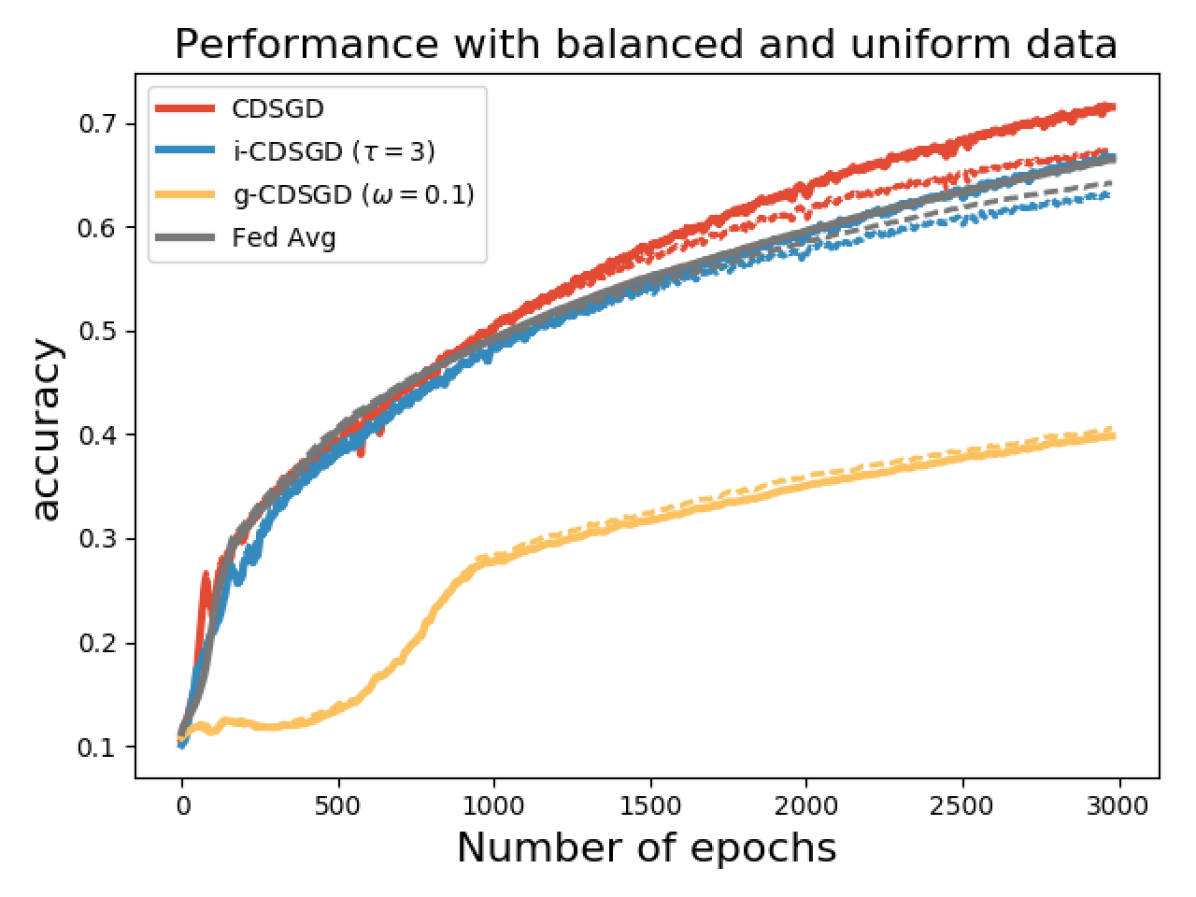
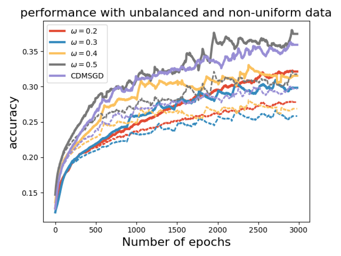
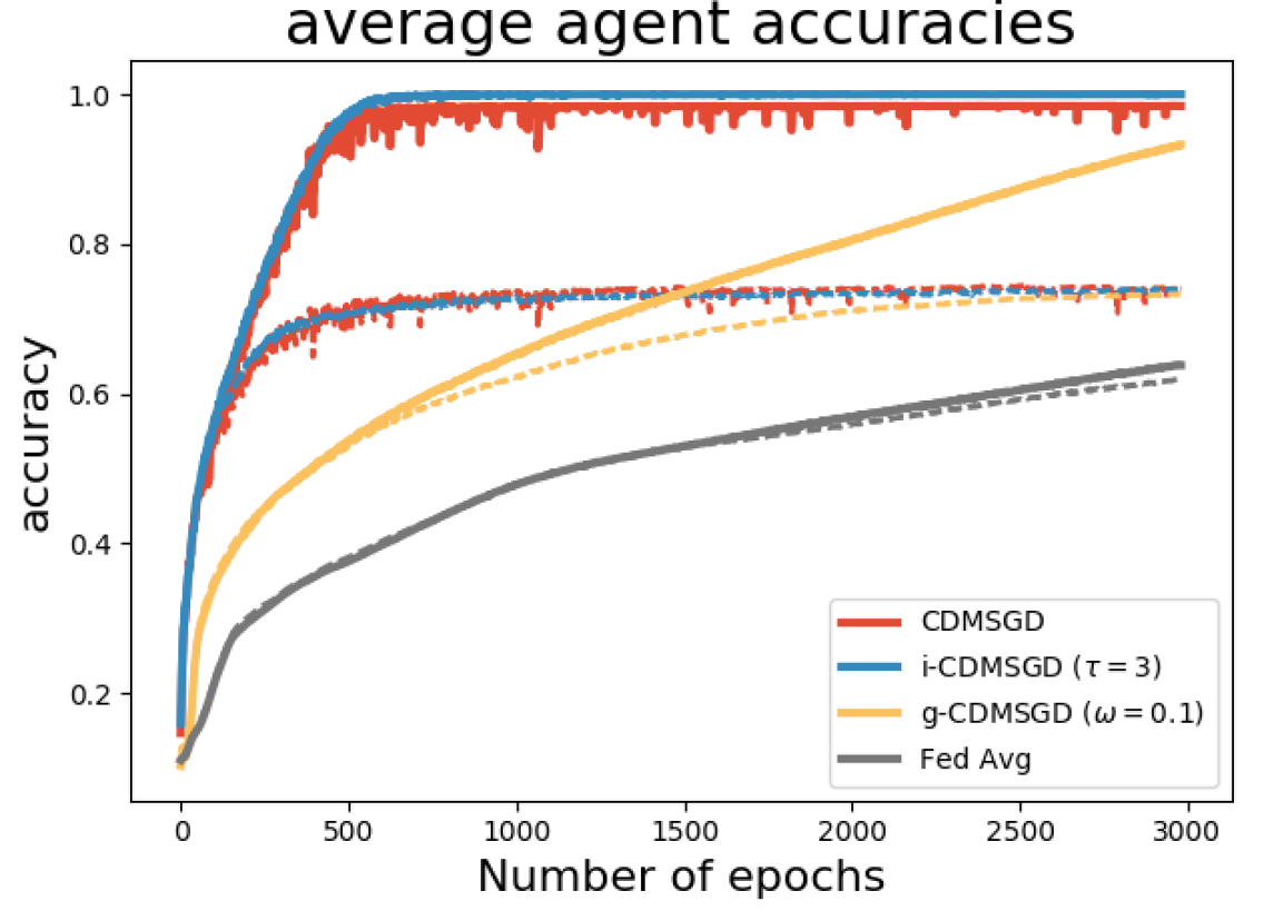
(a) Performance of different algorithms with unbalanced sample distribution among agents. (Dashed lines represent test accuracy & solid lines represent training accuracy.)
Refer to caption
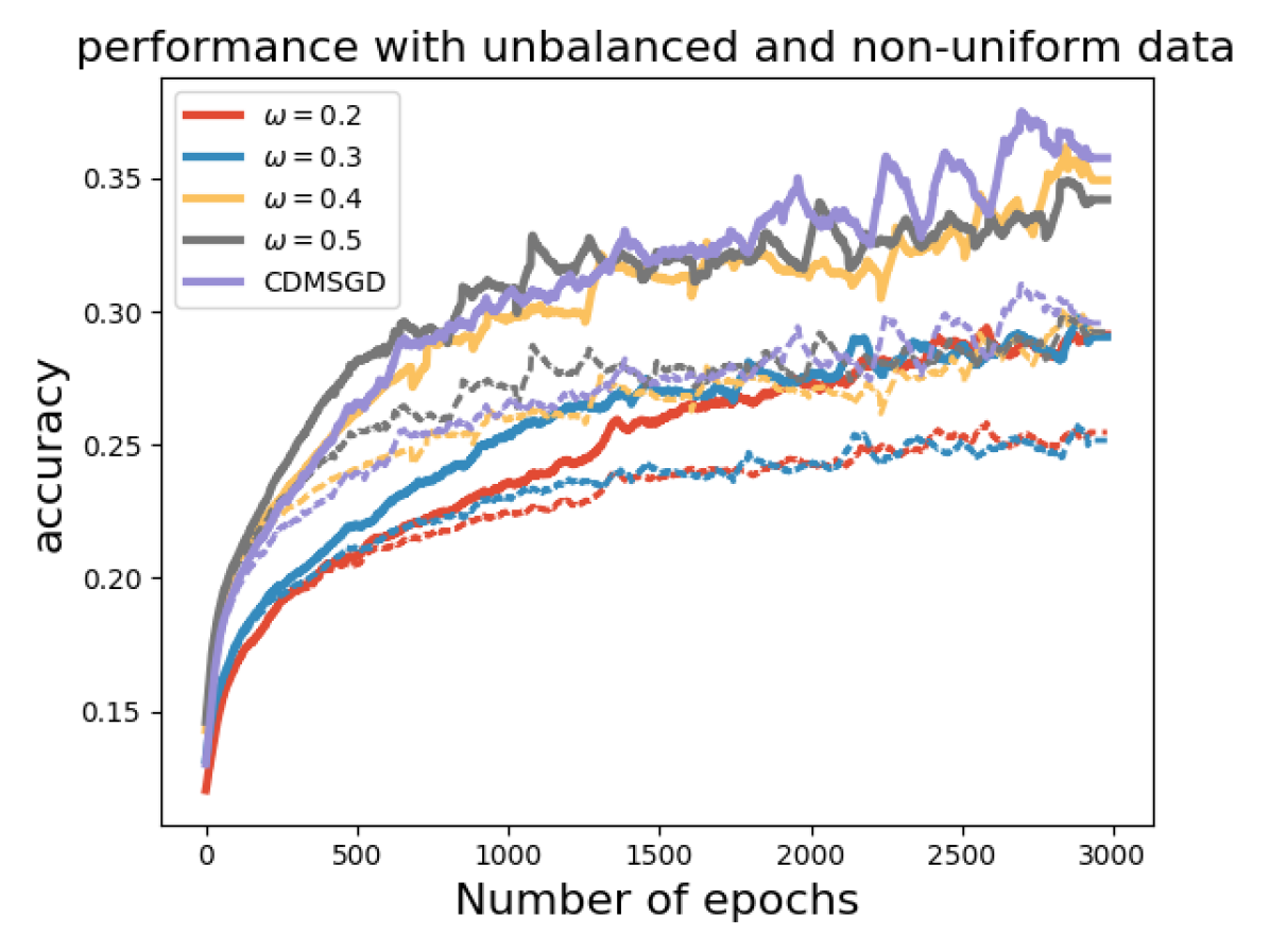
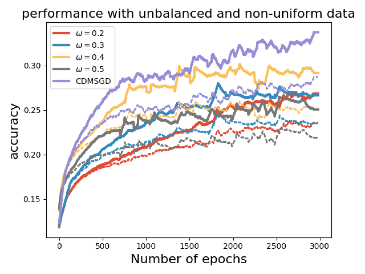
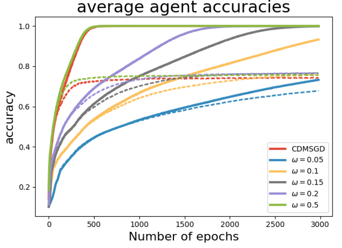
(b) Performance of g-CDMSGD for different ω𝜔\omega values. (Dashed lines represent test accuracy & solid lines represent training accuracy.)
Refer to caption
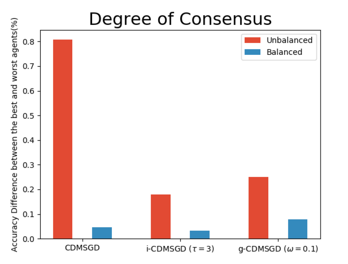
(c) The accuracy percentage difference between the best and the worst agents for different algorithms with unbalanced and balanced sample distribution among agents.
Refer to caption
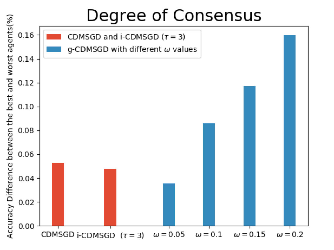
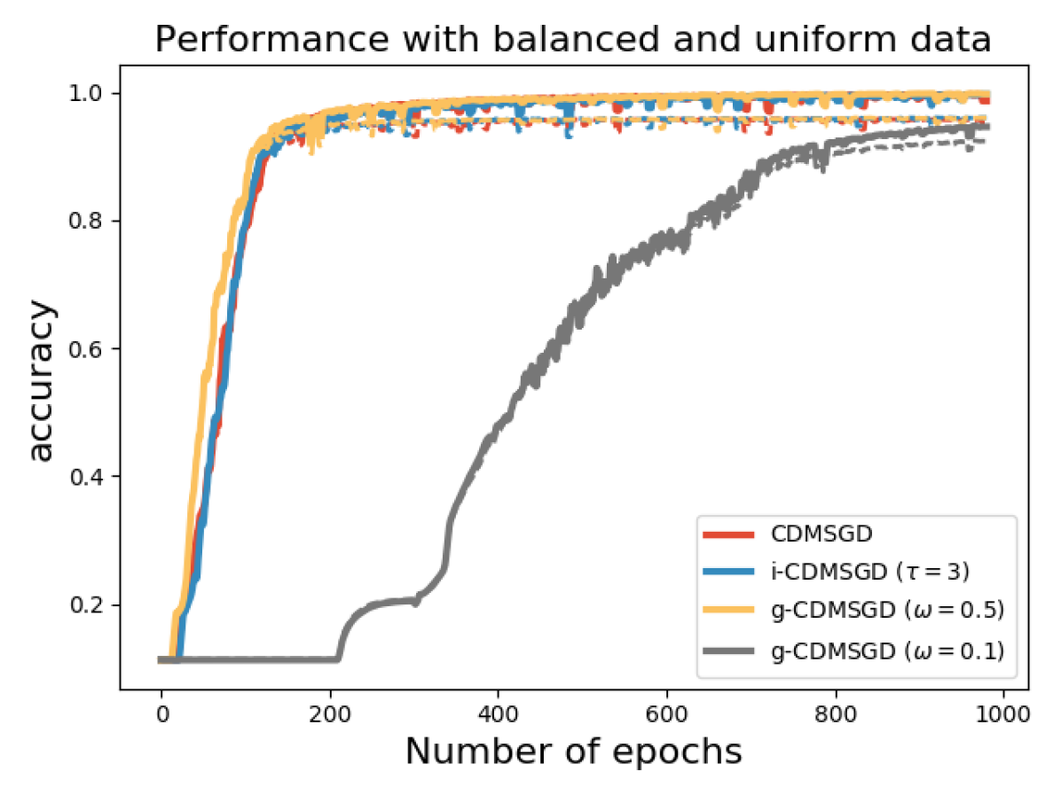
(d) The accuracy percentage difference between the best and the worst agents with balanced sample distribution for CDMSGD, i-CDMSGD and g-CDMSGD (varying ω𝜔\omega.)
Figure 2: Results from numerical experiments with CIFAR-10 data set

5   Experimental Results

We validate our algorithms via several experimental results using the CIFAR-10 image recognition dataset (with standard training and testing sets). The model adopted for the experiments is a deep convolutional neural network (CNN) (with ReLU activations) which includes 2 convolutional layers with 32 filters each followed by a max pooling layer, then 2 more convolutional layers with 64 filters each followed by another max pooling layer, and a dense layer with 512 units. The mini-batch size is set to 512, and step size is set to 0.01 in all experiments. All experiments were performed using Keras with TensorFlow [29, 30]. We use a sparse network topology with 5 agents. We use both balanced and unbalanced data sets for our experiments. In the balanced case, agents have an equal share of the entire training set. However, in the unbalanced case, agents have (randomly selected) unequal parts of the training set while making sure that each agent has at least half of the equal share amount of examples. We summarize our key experimental results in this section, with more details and results provided in the Supplementary Section A.4.

Performance of algorithms. In Figure 2(a), we compare the performance of the momentum variants of our proposed algorithms, i-CDMSGD and g-CDMSGD (with ω=0.1𝜔0.1\omega=0.1) with state-of-the art techniques such as CDMSGD and Federated Averaging using an unbalanced data set. All algorithms were run for 3000 epochs. Observing the average accuracy over all the agents for both training and test data, we note that i-CDMSGD can converge as fast as CDMSGD with lesser fluctuation in the performance across epochs. While being slower in convergence, g-CDMSGD acheves similar performance (with test data) with less fluctuation as well as smaller generalization gap (i.e., difference between training and testing accuracy). All algorithms significantly outperform Federated Averaging in terms of average accuracy. We also vary the tuning parameter ω𝜔\omega for g-CDMSGD to show (in Figure 2(b)) that it is able to achieve similar (or better) convergence rate as CDMSGD using higher ω𝜔\omega values with some sacrifice in terms of the generalization gap.

Degree of Consensus. One of the main contribution of our paper is to show that one can control the degree of consensus while maintaining average accuracy in distributed deep learning. We demonstrate this by observing the accuracy difference between the best and the worst performing agents (identified by computing the mean accuracy for the last 100 epochs). As shown in Figure 2(c), the degree of consensus is similar for all three algorithms for balanced data set, with i-CDMSGD performing slightly better than the rest. However, for an unbalanced set, both i-CDMSGD and g-CDMSGD perform significantly better compared to CDMSGD. Note, the degree of consensus can be further improved for g-CDMSGD using lower values of ω𝜔\omega as shown in Figure 2(d). However, the convergence becomes relatively slower as shown in Figure 2(b). We do not compare these results with the Federated Averaging algorithm as it performs a brute force consensus at every epoch using centralized parameter server. We also do not vary τ𝜏\tau as the doubly stochastic agent interaction matrix for the small agent population becomes stationary very quickly with a very small value of τ𝜏\tau. However, this will be explored in our future work with significantly bigger networks.

6   Conclusion and Future Work

For investigating the trade-off between consensus and optimality in distributed deep learning with constrained communication topology, this paper presents two new algorithms, called i-CDSGD and g-CDSGD and their momentum variants. We show the convergence properties for the proposed algorithms and the relationships between the hyperparameters and the consensus & optimality bounds. Theoretical and experimental comparison with the state-of-the-art algorithm called CDSGD, shows that i-CDSGD, and g-CDSGD can improve the degree of consensus among the agents while maintaining the average accuracy especially when there is data imbalance among the agents. Future research directions include learning with non-uniform data distributions among agents and time-varying networks.

References

  • [1] Yann LeCun, Yoshua Bengio, and Geoffrey Hinton. Deep learning. Nature, 521(7553):436--444, 2015.
  • [2] Benjamin Recht, Christopher Re, Stephen Wright, and Feng Niu. Hogwild: A lock-free approach to parallelizing stochastic gradient descent. In Advances in Neural Information Processing Systems, pages 693--701, 2011.
  • [3] Peter H Jin, Qiaochu Yuan, Forrest Iandola, and Kurt Keutzer. How to scale distributed deep learning? arXiv preprint arXiv:1611.04581, 2016.
  • [4] Ian Lenz, Honglak Lee, and Ashutosh Saxena. Deep learning for detecting robotic grasps. The International Journal of Robotics Research, 34(4-5):705--724, 2015.
  • [5] Jayavardhana Gubbi, Rajkumar Buyya, Slaven Marusic, and Marimuthu Palaniswami. Internet of things (iot): A vision, architectural elements, and future directions. Future generation computer systems, 29(7):1645--1660, 2013.
  • [6] Nicholas D Lane, Sourav Bhattacharya, Petko Georgiev, Claudio Forlivesi, and Fahim Kawsar. An early resource characterization of deep learning on wearables, smartphones and internet-of-things devices. In Proceedings of the 2015 International Workshop on Internet of Things towards Applications, pages 7--12. ACM, 2015.
  • [7] Nicholas D Lane and Petko Georgiev. Can deep learning revolutionize mobile sensing? In Proceedings of the 16th International Workshop on Mobile Computing Systems and Applications, pages 117--122. ACM, 2015.
  • [8] Jeffrey Dean, Greg Corrado, Rajat Monga, Kai Chen, Matthieu Devin, Mark Mao, Andrew Senior, Paul Tucker, Ke Yang, Quoc V Le, et al. Large scale distributed deep networks. In Advances in neural information processing systems, pages 1223--1231, 2012.
  • [9] Zhanhong Jiang, Aditya Balu, Chinmay Hegde, and Soumik Sarkar. Collaborative deep learning in fixed topology networks. Neural Information Processing Systems (NIPS), 2017.
  • [10] Mu Li, David G Andersen, Alexander J Smola, and Kai Yu. Communication efficient distributed machine learning with the parameter server. In Advances in Neural Information Processing Systems, pages 19--27, 2014.
  • [11] Dipankar Das, Sasikanth Avancha, Dheevatsa Mudigere, Karthikeyan Vaidynathan, Srinivas Sridharan, Dhiraj Kalamkar, Bharat Kaul, and Pradeep Dubey. Distributed deep learning using synchronous stochastic gradient descent. arXiv preprint arXiv:1602.06709, 2016.
  • [12] Xiangru Lian, Ce Zhang, Huan Zhang, Cho-Jui Hsieh, Wei Zhang, and Ji Liu. Can decentralized algorithms outperform centralized algorithms? a case study for decentralized parallel stochastic gradient descent. In Advances in Neural Information Processing Systems, pages 5336--5346, 2017.
  • [13] Albert S Berahas, Raghu Bollapragada, Nitish Shirish Keskar, and Ermin Wei. Balancing communication and computation in distributed optimization. arXiv preprint arXiv:1709.02999, 2017.
  • [14] Zhanhong Jiang, Kushal Mukherjee, and Soumik Sarkar. Generalised gossip-based subgradient method for distributed optimisation. International Journal of Control, pages 1--17, 2017.
  • [15] H Brendan McMahan, Eider Moore, Daniel Ramage, Seth Hampson, et al. Communication-efficient learning of deep networks from decentralized data. arXiv preprint arXiv:1602.05629, 2016.
  • [16] Kevin Scaman, Francis Bach, Sébastien Bubeck, Yin Tat Lee, and Laurent Massoulié. Optimal algorithms for smooth and strongly convex distributed optimization in networks. In International Conference on Machine Learning, pages 3027--3036, 2017.
  • [17] Guannan Qu and Na Li. Accelerated distributed nesterov gradient descent. arXiv preprint arXiv:1705.07176, 2017.
  • [18] Sixin Zhang, Anna E Choromanska, and Yann LeCun. Deep learning with elastic averaging sgd. In Advances in Neural Information Processing Systems, pages 685--693, 2015.
  • [19] Michael Blot, David Picard, Matthieu Cord, and Nicolas Thome. Gossip training for deep learning. arXiv preprint arXiv:1611.09726, 2016.
  • [20] Zheng Xu, Gavin Taylor, Hao Li, Mario Figueiredo, Xiaoming Yuan, and Tom Goldstein. Adaptive consensus admm for distributed optimization. In International Conference on Machine Learning, pages 3841--3850, 2017.
  • [21] Shuxin Zheng, Qi Meng, Taifeng Wang, Wei Chen, Nenghai Yu, Zhi-Ming Ma, and Tie-Yan Liu. Asynchronous stochastic gradient descent with delay compensation for distributed deep learning. In International Conference on Machine Learning, pages 4120--4129, 2017.
  • [22] Wenpeng Zhang, Peilin Zhao, Wenwu Zhu, Steven CH Hoi, and Tong Zhang. Projection-free distributed online learning in networks. In International Conference on Machine Learning, pages 4054--4062, 2017.
  • [23] Jianqiao Wangni, Jialei Wang, Ji Liu, and Tong Zhang. Gradient sparsification for communication-efficient distributed optimization. arXiv preprint arXiv:1710.09854, 2017.
  • [24] Wei Wen, Cong Xu, Feng Yan, Chunpeng Wu, Yandan Wang, Yiran Chen, and Hai Li. Terngrad: Ternary gradients to reduce communication in distributed deep learning. In Advances in Neural Information Processing Systems, pages 1508--1518, 2017.
  • [25] Konstantinos I Tsianos and Michael G Rabbat. Distributed strongly convex optimization. In Communication, Control, and Computing (Allerton), 2012 50th Annual Allerton Conference on, pages 593--600. IEEE, 2012.
  • [26] Ilya Sutskever, James Martens, George Dahl, and Geoffrey Hinton. On the importance of initialization and momentum in deep learning. In International conference on machine learning, pages 1139--1147, 2013.
  • [27] Shuang Song, Kamalika Chaudhuri, and Anand Sarwate. Learning from data with heterogeneous noise using sgd. pages 894--902, 2015.
  • [28] Léon Bottou, Frank E Curtis, and Jorge Nocedal. Optimization methods for large-scale machine learning. arXiv preprint arXiv:1606.04838, 2016.
  • [29] François Chollet et al. Keras, 2015.
  • [30] Martín Abadi, Paul Barham, Jianmin Chen, Zhifeng Chen, Andy Davis, Jeffrey Dean, Matthieu Devin, Sanjay Ghemawat, Geoffrey Irving, Michael Isard, et al. Tensorflow: A system for large-scale machine learning. In OSDI, volume 16, pages 265--283, 2016.
  • [31] Yurii Nesterov. Introductory lectures on convex optimization: A basic course, volume 87. Springer Science & Business Media, 2013.
  • [32] Atsushi Nitanda. Stochastic proximal gradient descent with acceleration techniques. In Advances in Neural Information Processing Systems, pages 1574--1582, 2014.

Appendix A Supplementary Materials

A.1   Omitted algorithms

Update rules for the momentum variant, i-CDMSGD. The compact form of i-CDMSGD is expressed as follows:

𝐲k+1=Θk+μ(ΘkΘk1)subscript𝐲𝑘1subscriptΘ𝑘𝜇subscriptΘ𝑘subscriptΘ𝑘1\displaystyle\mathbf{y}_{k+1}=\Theta_{k}+\mu(\Theta_{k}-\Theta_{k-1}) (25a)
Θk+1=𝐏τ𝐲k+1α𝐠(𝐲k+1).subscriptΘ𝑘1superscript𝐏𝜏subscript𝐲𝑘1𝛼𝐠subscript𝐲𝑘1\displaystyle\Theta_{k+1}=\mathbf{P}^{\tau}\mathbf{y}_{k+1}-\alpha\mathbf{g}(\mathbf{y}_{k+1}). (25b)

Rewriting the above equations yields:

Θk+1=𝐲k+1𝐲k+1+𝐏τ𝐲k+1α𝐠(𝐲k+1)subscriptΘ𝑘1subscript𝐲𝑘1subscript𝐲𝑘1superscript𝐏𝜏subscript𝐲𝑘1𝛼𝐠subscript𝐲𝑘1\displaystyle\Theta_{k+1}=\mathbf{y}_{k+1}-\mathbf{y}_{k+1}+\mathbf{P}^{\tau}\mathbf{y}_{k+1}-\alpha\mathbf{g}(\mathbf{y}_{k+1}) (26)
=𝐲k+1α(𝐠(𝐲k+1)+1α(INd𝐏τ)𝐲k+1).absentsubscript𝐲𝑘1𝛼𝐠subscript𝐲𝑘11𝛼subscript𝐼𝑁𝑑superscript𝐏𝜏subscript𝐲𝑘1\displaystyle=\mathbf{y}_{k+1}-\alpha(\mathbf{g}(\mathbf{y}_{k+1})+\frac{1}{\alpha}(I_{Nd}-\mathbf{P}^{\tau})\mathbf{y}_{k+1}).

Letting 𝒮(𝐲k+1)=𝐠(𝐲k+1)+1α(INd𝐏τ)𝒮subscript𝐲𝑘1𝐠subscript𝐲𝑘11𝛼subscript𝐼𝑁𝑑superscript𝐏𝜏\mathcal{S}(\mathbf{y}_{k+1})=\mathbf{g}(\mathbf{y}_{k+1})+\frac{1}{\alpha}(I_{Nd}-\mathbf{P}^{\tau}), we have

𝐲k+1=Θk+μ(ΘkΘk1),subscript𝐲𝑘1subscriptΘ𝑘𝜇subscriptΘ𝑘subscriptΘ𝑘1\displaystyle\mathbf{y}_{k+1}=\Theta_{k}+\mu(\Theta_{k}-\Theta_{k-1}), (27a)
Θk+1=𝐲k+1α𝒮(𝐲k+1).subscriptΘ𝑘1subscript𝐲𝑘1𝛼𝒮subscript𝐲𝑘1\displaystyle\Theta_{k+1}=\mathbf{y}_{k+1}-\alpha\mathcal{S}(\mathbf{y}_{k+1}). (27b)

A.1.1   Proofs of main lemmas

We repeat the statements of all lemmas and theorems for completeness.

Lemma 1: Let Assumptions 1 and 2 hold. The iterates of g-CDSGD (Algorithm 2) satisfy the following kfor-all𝑘\forall k\in\mathbb{N}:

𝔼[V(Θk+1)]𝔼delimited-[]𝑉subscriptΘ𝑘1\displaystyle\mathbb{E}[V(\Theta_{k+1})] V(Θk)𝑉subscriptΘ𝑘\displaystyle-V(\Theta_{k}) (28)
αV(Θk)T𝔼[𝒮(Θk)]absent𝛼𝑉superscriptsubscriptΘ𝑘𝑇𝔼delimited-[]𝒮subscriptΘ𝑘\displaystyle\leq-\alpha\nabla V(\Theta_{k})^{T}\mathbb{E}[\mathcal{S}(\Theta_{k})]
+γ^2α2𝔼[𝒮(Θk)2].^𝛾2superscript𝛼2𝔼delimited-[]superscriptnorm𝒮subscriptΘ𝑘2\displaystyle+\frac{\hat{\gamma}}{2}\alpha^{2}\mathbb{E}[\|\mathcal{S}(\Theta_{k})\|^{2}].
Proof.

By Assumption 1, the iterates generated by g-CDSGD satisfy:

V(\displaystyle V( Θk+1)V(Θk)\displaystyle\Theta_{k+1})-V(\Theta_{k}) (29)
V(Θk)T(Θk+1Θk)+12γ^Θk+1Θk2absent𝑉superscriptsubscriptΘ𝑘𝑇subscriptΘ𝑘1subscriptΘ𝑘12^𝛾superscriptnormsubscriptΘ𝑘1subscriptΘ𝑘2\displaystyle\leq\nabla V(\Theta_{k})^{T}(\Theta_{k+1}-\Theta_{k})+\frac{1}{2}\hat{\gamma}\|\Theta_{k+1}-\Theta_{k}\|^{2}
=αV(Θk)T𝒮(Θk)+12γ^α2𝒮(𝐱k)2.absent𝛼𝑉superscriptsubscriptΘ𝑘𝑇𝒮subscriptΘ𝑘12^𝛾superscript𝛼2superscriptnorm𝒮subscript𝐱𝑘2\displaystyle=-\alpha\nabla V(\Theta_{k})^{T}\nabla\mathcal{S}(\Theta_{k})+\frac{1}{2}\hat{\gamma}\alpha^{2}\|\nabla\mathcal{S}(\mathbf{x}_{k})\|^{2}.

Taking expectations on both sides, we can obtain

𝔼𝔼\displaystyle\mathbb{E} [V(Θk+1)V(Θk)]delimited-[]𝑉subscriptΘ𝑘1𝑉subscriptΘ𝑘\displaystyle[V(\Theta_{k+1})-V(\Theta_{k})] (30)
𝔼[αV(Θk)T𝒮(Θk)+12γ^α2𝒮(Θk)2].absent𝔼delimited-[]𝛼𝑉superscriptsubscriptΘ𝑘𝑇𝒮subscriptΘ𝑘12^𝛾superscript𝛼2superscriptnorm𝒮subscriptΘ𝑘2\displaystyle\leq\mathbb{E}[-\alpha\nabla V(\Theta_{k})^{T}\nabla\mathcal{S}(\Theta_{k})+\frac{1}{2}\hat{\gamma}\alpha^{2}\|\nabla\mathcal{S}(\Theta_{k})\|^{2}].

While V(Θk)𝑉subscriptΘ𝑘V(\Theta_{k}) is deterministic, V(Θk+1)𝑉subscriptΘ𝑘1V(\Theta_{k+1}) can be considered to be stochastic due to the random sampling aspect. Therefore, we have

𝔼𝔼\displaystyle\mathbb{E} [V(Θk+1)]V(Θk)delimited-[]𝑉subscriptΘ𝑘1𝑉subscriptΘ𝑘\displaystyle[V(\Theta_{k+1})]-V(\Theta_{k}) (31)
αV(Θk)T𝔼[𝒮(Θk)]+12γ^α2𝔼[𝒮(Θk)2],absent𝛼𝑉superscriptsubscriptΘ𝑘𝑇𝔼delimited-[]𝒮subscriptΘ𝑘12^𝛾superscript𝛼2𝔼delimited-[]superscriptnorm𝒮subscriptΘ𝑘2\displaystyle\leq-\alpha\nabla V(\Theta_{k})^{T}\mathbb{E}[\nabla\mathcal{S}(\Theta_{k})]+\frac{1}{2}\hat{\gamma}\alpha^{2}\mathbb{E}[\|\nabla\mathcal{S}(\Theta_{k})\|^{2}],

which completes the proof. ∎

Lemma 2: Let Assumptions 12, and 3 hold. The iterates of i-CDSGD (Algorithm 2) satisfy the following inequality kfor-all𝑘\forall k\in\mathbb{N}:

𝔼𝔼\displaystyle\mathbb{E} [V(Θk+1)]V(Θk)delimited-[]𝑉subscriptΘ𝑘1𝑉subscriptΘ𝑘\displaystyle[V(\Theta_{k+1})]-V(\Theta_{k}) (32)
(r1γ^2αBm)αV(Θk)2+γ^2α2B.absentsubscript𝑟1^𝛾2𝛼subscript𝐵𝑚𝛼superscriptnorm𝑉subscriptΘ𝑘2^𝛾2superscript𝛼2𝐵\displaystyle\leq-(r_{1}-\frac{\hat{\gamma}}{2}\alpha B_{m})\alpha\|\nabla V(\Theta_{k})\|^{2}+\frac{\hat{\gamma}}{2}\alpha^{2}B. (33)
Proof.

Recalling Lemma 1 and using Assumption 2 and Remark 1, we have

𝔼[V(Θk+1)]V(Θk)r1αV(Θk)2𝔼delimited-[]𝑉subscriptΘ𝑘1𝑉subscriptΘ𝑘subscript𝑟1𝛼superscriptnorm𝑉subscriptΘ𝑘2\displaystyle\mathbb{E}[V(\Theta_{k+1})]-V(\Theta_{k})\leq-r_{1}\alpha\|\nabla V(\Theta_{k})\|^{2} (34)
+γ^2α2𝔼[𝒮(Θk)2]r1αV(Θk)2^𝛾2superscript𝛼2𝔼delimited-[]superscriptnorm𝒮subscriptΘ𝑘2subscript𝑟1𝛼superscriptnorm𝑉subscriptΘ𝑘2\displaystyle+\frac{\hat{\gamma}}{2}\alpha^{2}\mathbb{E}[\|\nabla\mathcal{S}(\Theta_{k})\|^{2}]\leq-r_{1}\alpha\|\nabla V(\Theta_{k})\|^{2}
+γ^2α2(B+BmV(Θk)2)^𝛾2superscript𝛼2𝐵subscript𝐵𝑚superscriptnorm𝑉subscriptΘ𝑘2\displaystyle+\frac{\hat{\gamma}}{2}\alpha^{2}(B+B_{m}\|\nabla V(\Theta_{k})\|^{2})
=(r1γ^2αBm)αV(Θk)2+γ^2α2Babsentsubscript𝑟1^𝛾2𝛼subscript𝐵𝑚𝛼superscriptnorm𝑉subscriptΘ𝑘2^𝛾2superscript𝛼2𝐵\displaystyle=-(r_{1}-\frac{\hat{\gamma}}{2}\alpha B_{m})\alpha\|\nabla V(\Theta_{k})\|^{2}+\frac{\hat{\gamma}}{2}\alpha^{2}B

which completes the proof. ∎

Proposition 1: Let Assumptions 124 hold. The iterates of g-CDSGD (Algorithm 2) satisfy the following inequality kfor-all𝑘\forall k\in\mathbb{N}, when α𝛼\alpha satisfies Eq. 15,

𝔼[θkjsk]ωαh1λ^2,𝔼delimited-[]normsubscriptsuperscript𝜃𝑗𝑘subscript𝑠𝑘𝜔𝛼1subscript^𝜆2\mathbb{E}[\|\theta^{j}_{k}-s_{k}\|]\leq\frac{\omega\alpha h}{1-\hat{\lambda}_{2}}, (35)

where sk=1Nj=1Nθkjsubscript𝑠𝑘1𝑁superscriptsubscript𝑗1𝑁superscriptsubscript𝜃𝑘𝑗s_{k}=\frac{1}{N}\sum_{j=1}^{N}\theta_{k}^{j}, λ^2subscript^𝜆2\hat{\lambda}_{2} is the second-largest eigenvalue of the matrix 𝐐=(1ω)(ΠId)+ωINd𝐐1𝜔tensor-productΠsubscript𝐼𝑑𝜔subscript𝐼𝑁𝑑\mathbf{Q}=(1-\omega)(\Pi\otimes I_{d})+\omega I_{Nd}.

Proof.

Rewriting the expression 6 in another form yields Θk+1=𝐐Θkωα𝐠(Θk)subscriptΘ𝑘1𝐐subscriptΘ𝑘𝜔𝛼𝐠subscriptΘ𝑘\Theta_{k+1}=\mathbf{Q}\Theta_{k}-\omega\alpha\mathbf{g}(\Theta_{k}). Recursively applying the new form of Eq. 6 results in the following expression

Θk=ωαo=0k1𝐐k1o𝐠(Θk)subscriptΘ𝑘𝜔𝛼superscriptsubscript𝑜0𝑘1superscript𝐐𝑘1𝑜𝐠subscriptΘ𝑘\Theta_{k}=-\omega\alpha\sum_{o=0}^{k-1}\mathbf{Q}^{k-1-o}\mathbf{g}(\Theta_{k}) (36)

which follows from that the initial value of ΘksubscriptΘ𝑘\Theta_{k} is set 0. Let 𝐬k=[sk;sk;;sk]Ndsubscript𝐬𝑘subscript𝑠𝑘subscript𝑠𝑘subscript𝑠𝑘superscript𝑁𝑑\mathbf{s}_{k}=[s_{k};s_{k};...;s_{k}]\in\mathbb{R}^{Nd} such that 𝐬k=1Nd(𝟏Nd𝟏NdT)Θksubscript𝐬𝑘1𝑁𝑑subscript1𝑁𝑑superscriptsubscript1𝑁𝑑𝑇subscriptΘ𝑘\mathbf{s}_{k}=\frac{1}{Nd}(\mathbf{1}_{Nd}\mathbf{1}_{Nd}^{T})\Theta_{k}. Therefore, we have

θkjskΘk𝐬knormsuperscriptsubscript𝜃𝑘𝑗subscript𝑠𝑘normsubscriptΘ𝑘subscript𝐬𝑘\displaystyle\|\theta_{k}^{j}-s_{k}\|\leq\|\Theta_{k}-\mathbf{s}_{k}\| (37)
=Θk1Nd(𝟏Nd𝟏NdT)ΘkabsentnormsubscriptΘ𝑘1𝑁𝑑subscript1𝑁𝑑superscriptsubscript1𝑁𝑑𝑇subscriptΘ𝑘\displaystyle=\|\Theta_{k}-\frac{1}{Nd}(\mathbf{1}_{Nd}\mathbf{1}_{Nd}^{T})\Theta_{k}\|
=ωαo=0k1𝐐k1o𝐠(Θo)\displaystyle=\|-\omega\alpha\sum_{o=0}^{k-1}\mathbf{Q}^{k-1-o}\mathbf{g}(\Theta_{o})
+ωαo=0k11Nd(𝟏Nd𝟏NdT𝐐k1o)𝐠(Θo)\displaystyle~{}~{}~{}~{}~{}+\omega\alpha\sum_{o=0}^{k-1}\frac{1}{Nd}(\mathbf{1}_{Nd}\mathbf{1}_{Nd}^{T}\mathbf{Q}^{k-1-o})\mathbf{g}(\Theta_{o})\|
=ωαo=0k1𝐐k1o𝐠(Θo)\displaystyle=\|-\omega\alpha\sum_{o=0}^{k-1}\mathbf{Q}^{k-1-o}\mathbf{g}(\Theta_{o})
+ωαo=0k11Nd(𝟏Nd𝟏NdT)𝐠(Θk)\displaystyle~{}~{}~{}~{}~{}+\omega\alpha\sum_{o=0}^{k-1}\frac{1}{Nd}(\mathbf{1}_{Nd}\mathbf{1}_{Nd}^{T})\mathbf{g}(\Theta_{k})\|
=ωαo=0k1(𝐐k1o1Nd𝟏Nd𝟏NdT)𝐠(Θo)absent𝜔𝛼normsuperscriptsubscript𝑜0𝑘1superscript𝐐𝑘1𝑜1𝑁𝑑subscript1𝑁𝑑superscriptsubscript1𝑁𝑑𝑇𝐠subscriptΘ𝑜\displaystyle=\omega\alpha\|\sum_{o=0}^{k-1}(\mathbf{Q}^{k-1-o}-\frac{1}{Nd}\mathbf{1}_{Nd}\mathbf{1}_{Nd}^{T})\mathbf{g}(\Theta_{o})\|
ωαo=0k1𝐐k1o1Nd𝟏Nd𝟏NdT𝐠(Θo)absent𝜔𝛼superscriptsubscript𝑜0𝑘1normsuperscript𝐐𝑘1𝑜1𝑁𝑑subscript1𝑁𝑑superscriptsubscript1𝑁𝑑𝑇norm𝐠subscriptΘ𝑜\displaystyle\leq\omega\alpha\sum_{o=0}^{k-1}\|\mathbf{Q}^{k-1-o}-\frac{1}{Nd}\mathbf{1}_{Nd}\mathbf{1}_{Nd}^{T}\|\|\mathbf{g}(\Theta_{o})\|
=ωαo=0k1λ^2k1o𝐠(Θo),absent𝜔𝛼superscriptsubscript𝑜0𝑘1superscriptsubscript^𝜆2𝑘1𝑜norm𝐠subscriptΘ𝑜\displaystyle=\omega\alpha\sum_{o=0}^{k-1}\hat{\lambda}_{2}^{k-1-o}\|\mathbf{g}(\Theta_{o})\|,

where the third equality follows from that 1Nd𝟏Nd𝟏NdT𝐐=1Nd𝟏Nd𝟏NdT1𝑁𝑑subscript1𝑁𝑑superscriptsubscript1𝑁𝑑𝑇𝐐1𝑁𝑑subscript1𝑁𝑑superscriptsubscript1𝑁𝑑𝑇\frac{1}{Nd}\mathbf{1}_{Nd}\mathbf{1}_{Nd}^{T}\mathbf{Q}=\frac{1}{Nd}\mathbf{1}_{Nd}\mathbf{1}_{Nd}^{T}, the second inequality is obtained by using Cauchy-Schwartz inequality, λ^2<1subscript^𝜆21\hat{\lambda}_{2}\textless 1.

Therefore, the following relationships can be obtained:

𝔼[θkjsk]𝔼delimited-[]normsuperscriptsubscript𝜃𝑘𝑗subscript𝑠𝑘\displaystyle\mathbb{E}[\|\theta_{k}^{j}-s_{k}\|] ωα𝔼[o=0k1λ^2k1o𝐠(Θo)]absent𝜔𝛼𝔼delimited-[]superscriptsubscript𝑜0𝑘1superscriptsubscript^𝜆2𝑘1𝑜norm𝐠subscriptΘ𝑜\displaystyle\leq\omega\alpha\mathbb{E}[\sum_{o=0}^{k-1}\hat{\lambda}_{2}^{k-1-o}\|\mathbf{g}(\Theta_{o})\|] (38)
=ωαo=0k1λ^2k1o𝔼[𝐠(Θo)]absent𝜔𝛼superscriptsubscript𝑜0𝑘1superscriptsubscript^𝜆2𝑘1𝑜𝔼delimited-[]norm𝐠subscriptΘ𝑜\displaystyle=\omega\alpha\sum_{o=0}^{k-1}\hat{\lambda}_{2}^{k-1-o}\mathbb{E}[\|\mathbf{g}(\Theta_{o})\|]
ωαh1λ^2,absent𝜔𝛼1subscript^𝜆2\displaystyle\leq\frac{\omega\alpha h}{1-\hat{\lambda}_{2}},

which completes the proof. ∎

Similarly, the consensus bound for i-CDSGD is shown as follows.

Proposition 2: Let Assumptions 124 hold. The iterates of i-CDSGD (Algorithm 1) satisfy the following inequality kfor-all𝑘\forall k\in\mathbb{N}, when α𝛼\alpha satisfies 0<αr1(1λNτ)BmγmBm0𝛼subscript𝑟11superscriptsubscript𝜆𝑁𝜏subscript𝐵𝑚subscript𝛾𝑚subscript𝐵𝑚0\textless\alpha\leq\frac{r_{1}-(1-\lambda_{N}^{\tau})B_{m}}{\gamma_{m}B_{m}}:

𝔼[θkjsk]αh1λ2τ𝔼delimited-[]normsubscriptsuperscript𝜃𝑗𝑘subscript𝑠𝑘𝛼1superscriptsubscript𝜆2𝜏\mathbb{E}[\|\theta^{j}_{k}-s_{k}\|]\leq\frac{\alpha h}{1-\lambda_{2}^{\tau}} (39)

where sk=1Nj=1Nθkjsubscript𝑠𝑘1𝑁superscriptsubscript𝑗1𝑁superscriptsubscript𝜃𝑘𝑗s_{k}=\frac{1}{N}\sum_{j=1}^{N}\theta_{k}^{j}.

Proof.

Rewriting Equation (5) yields

Θk+1=𝐏τΘkα𝐠(Θk).subscriptΘ𝑘1superscript𝐏𝜏subscriptΘ𝑘𝛼𝐠subscriptΘ𝑘\Theta_{k+1}=\mathbf{P}^{\tau}\Theta_{k}-\alpha\mathbf{g}(\Theta_{k}).

Recursively applying the new form of Equation (5) results in the following expression:

Θk=αo=0k1𝐏τ(k1o)𝐠(Θk)subscriptΘ𝑘𝛼superscriptsubscript𝑜0𝑘1superscript𝐏𝜏𝑘1𝑜𝐠subscriptΘ𝑘\Theta_{k}=-\alpha\sum_{o=0}^{k-1}\mathbf{P}^{\tau(k-1-o)}\mathbf{g}(\Theta_{k}) (40)

which follows from the fact that that the initial value of ΘksubscriptΘ𝑘\Theta_{k} is set 0.

Let 𝐬k=[sk;sk;;sk]Ndsubscript𝐬𝑘subscript𝑠𝑘subscript𝑠𝑘subscript𝑠𝑘superscript𝑁𝑑\mathbf{s}_{k}=[s_{k};s_{k};...;s_{k}]\in\mathbb{R}^{Nd} such that

𝐬k=1Nd(𝟏Nd𝟏NdT)Θk.subscript𝐬𝑘1𝑁𝑑subscript1𝑁𝑑superscriptsubscript1𝑁𝑑𝑇subscriptΘ𝑘\mathbf{s}_{k}=\frac{1}{Nd}(\mathbf{1}_{Nd}\mathbf{1}_{Nd}^{T})\Theta_{k}.

Therefore, we have:

θkjsknormsuperscriptsubscript𝜃𝑘𝑗subscript𝑠𝑘\displaystyle\|\theta_{k}^{j}-s_{k}\| Θk𝐬kabsentnormsubscriptΘ𝑘subscript𝐬𝑘\displaystyle\leq\|\Theta_{k}-\mathbf{s}_{k}\| (41)
=Θk1Nd(𝟏Nd𝟏NdT)ΘkabsentnormsubscriptΘ𝑘1𝑁𝑑subscript1𝑁𝑑superscriptsubscript1𝑁𝑑𝑇subscriptΘ𝑘\displaystyle=\|\Theta_{k}-\frac{1}{Nd}(\mathbf{1}_{Nd}\mathbf{1}_{Nd}^{T})\Theta_{k}\|
=αo=0k1𝐏τ(k1o)𝐠(Θo)\displaystyle=\|-\alpha\sum_{o=0}^{k-1}\mathbf{P}^{\tau(k-1-o)}\mathbf{g}(\Theta_{o})
+αo=0k11Nd(𝟏Nd𝟏NdT𝐏τ(k1o))𝐠(Θo)\displaystyle~{}~{}~{}~{}~{}+\alpha\sum_{o=0}^{k-1}\frac{1}{Nd}(\mathbf{1}_{Nd}\mathbf{1}_{Nd}^{T}\mathbf{P}^{\tau(k-1-o)})\mathbf{g}(\Theta_{o})\|
=αo=0k1𝐏τ(k1o)𝐠(Θo)\displaystyle=\|-\alpha\sum_{o=0}^{k-1}\mathbf{P}^{\tau(k-1-o)}\mathbf{g}(\Theta_{o})
+αo=0k11Nd(𝟏Nd𝟏NdT)𝐠(Θk)\displaystyle~{}~{}~{}~{}~{}+\alpha\sum_{o=0}^{k-1}\frac{1}{Nd}(\mathbf{1}_{Nd}\mathbf{1}_{Nd}^{T})\mathbf{g}(\Theta_{k})\|
=αo=0k1(𝐏τ(k1o)1Nd𝟏Nd𝟏NdT)𝐠(Θo)absent𝛼normsuperscriptsubscript𝑜0𝑘1superscript𝐏𝜏𝑘1𝑜1𝑁𝑑subscript1𝑁𝑑superscriptsubscript1𝑁𝑑𝑇𝐠subscriptΘ𝑜\displaystyle=\alpha\|\sum_{o=0}^{k-1}(\mathbf{P}^{\tau(k-1-o)}-\frac{1}{Nd}\mathbf{1}_{Nd}\mathbf{1}_{Nd}^{T})\mathbf{g}(\Theta_{o})\|
αo=0k1𝐏τ(k1o)1Nd𝟏Nd𝟏NdT𝐠(Θo)absent𝛼superscriptsubscript𝑜0𝑘1normsuperscript𝐏𝜏𝑘1𝑜1𝑁𝑑subscript1𝑁𝑑superscriptsubscript1𝑁𝑑𝑇norm𝐠subscriptΘ𝑜\displaystyle\leq\alpha\sum_{o=0}^{k-1}\|\mathbf{P}^{\tau(k-1-o)}-\frac{1}{Nd}\mathbf{1}_{Nd}\mathbf{1}_{Nd}^{T}\|\|\mathbf{g}(\Theta_{o})\|
=αo=0k1λ2τ(k1o)𝐠(Θo),absent𝛼superscriptsubscript𝑜0𝑘1superscriptsubscript𝜆2𝜏𝑘1𝑜norm𝐠subscriptΘ𝑜\displaystyle=\alpha\sum_{o=0}^{k-1}\lambda_{2}^{\tau(k-1-o)}\|\mathbf{g}(\Theta_{o})\|,

where the third equality follows from that 1N𝟏N𝟏NT𝐏=1N𝟏N𝟏NT1𝑁subscript1𝑁superscriptsubscript1𝑁𝑇𝐏1𝑁subscript1𝑁superscriptsubscript1𝑁𝑇\frac{1}{N}\mathbf{1}_{N}\mathbf{1}_{N}^{T}\mathbf{P}=\frac{1}{N}\mathbf{1}_{N}\mathbf{1}_{N}^{T}, and the second inequality is obtained by using the Cauchy-Schwartz inequality. Therefore,

𝔼[θkjsk]𝔼delimited-[]normsuperscriptsubscript𝜃𝑘𝑗subscript𝑠𝑘\displaystyle\mathbb{E}[\|\theta_{k}^{j}-s_{k}\|] α𝔼[o=0k1λ2τ(k1o)𝐠(Θo)]absent𝛼𝔼delimited-[]superscriptsubscript𝑜0𝑘1superscriptsubscript𝜆2𝜏𝑘1𝑜norm𝐠subscriptΘ𝑜\displaystyle\leq\alpha\mathbb{E}[\sum_{o=0}^{k-1}\lambda_{2}^{\tau(k-1-o)}\|\mathbf{g}(\Theta_{o})\|] (42)
=αo=0k1λ2τ(k1o)𝔼[𝐠(Θo)]absent𝛼superscriptsubscript𝑜0𝑘1superscriptsubscript𝜆2𝜏𝑘1𝑜𝔼delimited-[]norm𝐠subscriptΘ𝑜\displaystyle=\alpha\sum_{o=0}^{k-1}\lambda_{2}^{\tau(k-1-o)}\mathbb{E}[\|\mathbf{g}(\Theta_{o})\|]
αh1λ2τ.absent𝛼1superscriptsubscript𝜆2𝜏\displaystyle\leq\frac{\alpha h}{1-\lambda_{2}^{\tau}}.

which completes the proof. ∎

We next show the main results for g-CDSGD and i-CDSGD with both strongly convex and nonconvex objective functions.

Theorem 1 (Convergence of g-CDSGD to global optimum, strongly convex case): Let Assumptions 12 and 3 hold. When the step size satisfies Eq. 15, the iterates of g-CDSGD (Algorithm 2) satisfy the following inequality kfor-all𝑘\forall k\in\mathbb{N}:

𝔼[Dk]C1k1D1+C2q=0k1C1q𝔼delimited-[]subscript𝐷𝑘superscriptsubscript𝐶1𝑘1subscript𝐷1subscript𝐶2superscriptsubscript𝑞0𝑘1superscriptsubscript𝐶1𝑞\mathbb{E}[D_{k}]\leq C_{1}^{k-1}D_{1}+C_{2}\sum_{q=0}^{k-1}C_{1}^{q} (43)

where Dk=V(Θk)V,C1=1(ωαHm+1ω2(1λ2))r1,C2=(α2γmω+α(1ω)(1λN))B2formulae-sequencesubscript𝐷𝑘𝑉subscriptΘ𝑘superscript𝑉formulae-sequencesubscript𝐶11𝜔𝛼subscript𝐻𝑚1𝜔21subscript𝜆2subscript𝑟1subscript𝐶2superscript𝛼2subscript𝛾𝑚𝜔𝛼1𝜔1subscript𝜆𝑁𝐵2D_{k}=V(\Theta_{k})-V^{*},C_{1}=1-(\omega\alpha H_{m}+\frac{1-\omega}{2}(1-\lambda_{2}))r_{1},C_{2}=\frac{(\alpha^{2}\gamma_{m}\omega+\alpha(1-\omega)(1-\lambda_{N}))B}{2}.

Proof.

Recalling Lemma 2 and using Definition 1 yield:

𝔼[V\displaystyle\mathbb{E}[V (Θk+1)]V(Θk)\displaystyle(\Theta_{k+1})]-V(\Theta_{k}) (44)
(r1γ^2αBm)αV(Θk)2absentsubscript𝑟1^𝛾2𝛼subscript𝐵𝑚𝛼superscriptnorm𝑉subscriptΘ𝑘2\displaystyle\leq-(r_{1}-\frac{\hat{\gamma}}{2}\alpha B_{m})\alpha\|\nabla V(\Theta_{k})\|^{2}
+γ^2α2B12αr1(Θk)2+α2γ^B2^𝛾2superscript𝛼2𝐵12𝛼subscript𝑟1superscriptnormsubscriptΘ𝑘2superscript𝛼2^𝛾𝐵2\displaystyle+\frac{\hat{\gamma}}{2}\alpha^{2}B\leq-\frac{1}{2}\alpha r_{1}\|\nabla(\Theta_{k})\|^{2}+\frac{\alpha^{2}\hat{\gamma}B}{2}
αr1H^(V(Θk)V)+α2γ^B2.absent𝛼subscript𝑟1^𝐻𝑉subscriptΘ𝑘superscript𝑉superscript𝛼2^𝛾𝐵2\displaystyle\leq-\alpha r_{1}\hat{H}(V(\Theta_{k})-V^{*})+\frac{\alpha^{2}\hat{\gamma}B}{2}.

The second inequality follows from that αr1γ^Bm𝛼subscript𝑟1^𝛾subscript𝐵𝑚\alpha\leq\frac{r_{1}}{\hat{\gamma}B_{m}}, which is implied by Eq. 15. The expectation taken in the above inequalities is only related to θk+1subscript𝜃𝑘1\theta_{k+1}. Hence, recursively taking the expectation and subtracting Vsuperscript𝑉V^{*} from both sides, we get:

𝔼[V(Θk+1)V](1αH^r1)𝔼[V(Θk)V]+α2γ^B2.𝔼delimited-[]𝑉subscriptΘ𝑘1superscript𝑉1𝛼^𝐻subscript𝑟1𝔼delimited-[]𝑉subscriptΘ𝑘superscript𝑉superscript𝛼2^𝛾𝐵2\mathbb{E}[V(\Theta_{k+1})-V^{*}]\leq(1-\alpha\hat{H}r_{1})\mathbb{E}[V(\Theta_{k})-V^{*}]+\frac{\alpha^{2}\hat{\gamma}B}{2}. (45)

As 0<αH^r1H^r12γ^BmH^r12γ^r12=H^γ^10𝛼^𝐻subscript𝑟1^𝐻superscriptsubscript𝑟12^𝛾subscript𝐵𝑚^𝐻superscriptsubscript𝑟12^𝛾superscriptsubscript𝑟12^𝐻^𝛾10\textless\alpha\hat{H}r_{1}\leq\frac{\hat{H}r_{1}^{2}}{\hat{\gamma}B_{m}}\leq\frac{\hat{H}r_{1}^{2}}{\hat{\gamma}r_{1}^{2}}=\frac{\hat{H}}{\hat{\gamma}}\leq 1, the conclusion follows by applying Eq. 1 recursively through iteration k𝑘k\in\mathbb{N} and letting Dk=V(Θk)V,C1=1(ωαHm+1ω2(1λ2))r1,C2=(α2γmω+α(1ω)(1λN))B2formulae-sequencesubscript𝐷𝑘𝑉subscriptΘ𝑘superscript𝑉formulae-sequencesubscript𝐶11𝜔𝛼subscript𝐻𝑚1𝜔21subscript𝜆2subscript𝑟1subscript𝐶2superscript𝛼2subscript𝛾𝑚𝜔𝛼1𝜔1subscript𝜆𝑁𝐵2D_{k}=V(\Theta_{k})-V^{*},C_{1}=1-(\omega\alpha H_{m}+\frac{1-\omega}{2}(1-\lambda_{2}))r_{1},C_{2}=\frac{(\alpha^{2}\gamma_{m}\omega+\alpha(1-\omega)(1-\lambda_{N}))B}{2}. ∎

Theorem 2 (Convergence of i-CDSGD to global optimum, strongly convex case) Let Assumptions 12 and 3 hold. When the step size satisfies 0<αr1(1λNτ)BmγmBm0𝛼subscript𝑟11superscriptsubscript𝜆𝑁𝜏subscript𝐵𝑚subscript𝛾𝑚subscript𝐵𝑚0\textless\alpha\leq\frac{r_{1}-(1-\lambda_{N}^{\tau})B_{m}}{\gamma_{m}B_{m}}, the iterates of i-CDSGD (Algorithm 1) satisfy the following inequality kfor-all𝑘\forall k\in\mathbb{N}:

𝔼[Dk]C3k1D1+C4q=0k1C3q𝔼delimited-[]subscript𝐷𝑘superscriptsubscript𝐶3𝑘1subscript𝐷1subscript𝐶4superscriptsubscript𝑞0𝑘1superscriptsubscript𝐶3𝑞\mathbb{E}[D_{k}]\leq C_{3}^{k-1}D_{1}+C_{4}\sum_{q=0}^{k-1}C_{3}^{q} (46)

where Dk=V(Θk)V,C3=1(αHm+12(1λ2τ))r1,C4=(α2γm+α(1λNτ))B2formulae-sequencesubscript𝐷𝑘𝑉subscriptΘ𝑘superscript𝑉formulae-sequencesubscript𝐶31𝛼subscript𝐻𝑚121superscriptsubscript𝜆2𝜏subscript𝑟1subscript𝐶4superscript𝛼2subscript𝛾𝑚𝛼1superscriptsubscript𝜆𝑁𝜏𝐵2D_{k}=V(\Theta_{k})-V^{*},C_{3}=1-(\alpha H_{m}+\frac{1}{2}(1-\lambda_{2}^{\tau}))r_{1},C_{4}=\frac{(\alpha^{2}\gamma_{m}+\alpha(1-\lambda_{N}^{\tau}))B}{2}.

Proof.

We omit the proof here and one can easily get it following the proof techniques shown for Theorem 1. The desired result is obtained by replacing C1subscript𝐶1C_{1} with C3subscript𝐶3C_{3} and C2subscript𝐶2C_{2} with C4subscript𝐶4C_{4}, respectively. ∎

Theorem 3 (Convergence of g-CDSGD to a first-order stationary point, non-convex case): Let Assumptions 12, and 3 hold. When the step size satisfies Eq. 15, the iterates of g-CDSGD (Algorithm 2) satisfy the following inequality Kfor-all𝐾\forall K\in\mathbb{N}:

𝔼[\displaystyle\mathbb{E}[ 1Kk=1KV(Θk)2]\displaystyle\frac{1}{K}\sum_{k=1}^{K}\|\nabla V(\Theta_{k})\|^{2}] (47)
(ωγmα+(1ω)(1λN))Br1+2(V(Θ1)Vinf)Kr1αabsent𝜔subscript𝛾𝑚𝛼1𝜔1subscript𝜆𝑁𝐵subscript𝑟12𝑉subscriptΘ1subscript𝑉inf𝐾subscript𝑟1𝛼\displaystyle\leq\frac{(\omega\gamma_{m}\alpha+(1-\omega)(1-\lambda_{N}))B}{r_{1}}+\frac{2(V(\Theta_{1})-V_{\text{inf}})}{Kr_{1}\alpha}
Proof.

Recalling Lemma 2 and taking expectations on both sides lead to the following relation:

𝔼[V(\displaystyle\mathbb{E}[V( Θk+1)]𝔼[V(Θk)]\displaystyle\Theta_{k+1})]-\mathbb{E}[V(\Theta_{k})] (48)
(r1γ^αBm2)α𝔼[V(Θk)2]+γ^α2B2.absentsubscript𝑟1^𝛾𝛼subscript𝐵𝑚2𝛼𝔼delimited-[]superscriptnorm𝑉subscriptΘ𝑘2^𝛾superscript𝛼2𝐵2\displaystyle\leq-(r_{1}-\frac{\hat{\gamma}\alpha B_{m}}{2})\alpha\mathbb{E}[\|\nabla V(\Theta_{k})\|^{2}]+\frac{\hat{\gamma}\alpha^{2}B}{2}.

If the step size is such that αr1γ^Bm𝛼subscript𝑟1^𝛾subscript𝐵𝑚\alpha\leq\frac{r_{1}}{\hat{\gamma}B_{m}}, we get:

𝔼[V(Θk+1)]𝔼[V(Θk)]r1α2𝔼[V(Θk)2]+α2γ^B2.𝔼delimited-[]𝑉subscriptΘ𝑘1𝔼delimited-[]𝑉subscriptΘ𝑘subscript𝑟1𝛼2𝔼delimited-[]superscriptnorm𝑉subscriptΘ𝑘2superscript𝛼2^𝛾𝐵2\mathbb{E}[V(\Theta_{k+1})]-\mathbb{E}[V(\Theta_{k})]\leq-\frac{r_{1}\alpha}{2}\mathbb{E}[\|\nabla V(\Theta_{k})\|^{2}]+\frac{\alpha^{2}\hat{\gamma}B}{2}. (49)

Applying the above inequality from 1 to K𝐾K and summing them up can give the following relation

VinfV(Θ1)subscript𝑉inf𝑉subscriptΘ1\displaystyle V_{\text{inf}}-V(\Theta_{1}) 𝔼[V(Θk+1)]V(Θ1)absent𝔼delimited-[]𝑉subscriptΘ𝑘1𝑉subscriptΘ1\displaystyle\leq\mathbb{E}[V(\Theta_{k+1})]-V(\Theta_{1}) (50)
r1α2k=1m𝔼[V(Θk)2]+mα2γ^B2.absentsubscript𝑟1𝛼2superscriptsubscript𝑘1𝑚𝔼delimited-[]superscriptnorm𝑉subscriptΘ𝑘2𝑚superscript𝛼2^𝛾𝐵2\displaystyle\leq-\frac{r_{1}\alpha}{2}\sum_{k=1}^{m}\mathbb{E}[\|\nabla V(\Theta_{k})\|^{2}]+\frac{m\alpha^{2}\hat{\gamma}B}{2}.

The last inequality follows from the Assumption 3. Rearrangement of the above inequality, substituting γ^=ωγm+α1(1ω)(1λN)^𝛾𝜔subscript𝛾𝑚superscript𝛼11𝜔1subscript𝜆𝑁\hat{\gamma}=\omega\gamma_{m}+\alpha^{-1}(1-\omega)(1-\lambda_{N}), and dividing by K𝐾K yields the desired result. ∎

Theorem 4 (Convergence of i-CDSGD to a first-order stationary point, non-convex case): Let Assumptions 12, and 3 hold. When the step size satisfies 0<αr1(1λNτ)BmγmBm0𝛼subscript𝑟11superscriptsubscript𝜆𝑁𝜏subscript𝐵𝑚subscript𝛾𝑚subscript𝐵𝑚0\textless\alpha\leq\frac{r_{1}-(1-\lambda_{N}^{\tau})B_{m}}{\gamma_{m}B_{m}}, the iterates of i-CDSGD (Algorithm 1) satisfy the following inequality Kfor-all𝐾\forall K\in\mathbb{N}:

𝔼[\displaystyle\mathbb{E}[ 1Kk=1KV(Θk)2]\displaystyle\frac{1}{K}\sum_{k=1}^{K}\|\nabla V(\Theta_{k})\|^{2}] (51)
(γmα+(1λNτ))Br1+2(V(Θ1)Vinf)Kr1αabsentsubscript𝛾𝑚𝛼1superscriptsubscript𝜆𝑁𝜏𝐵subscript𝑟12𝑉subscriptΘ1subscript𝑉inf𝐾subscript𝑟1𝛼\displaystyle\leq\frac{(\gamma_{m}\alpha+(1-\lambda_{N}^{\tau}))B}{r_{1}}+\frac{2(V(\Theta_{1})-V_{\text{inf}})}{Kr_{1}\alpha}
Proof.

The proof for this theorem is rather similar to the one provided for Theorem 3 above, and we omit the details. ∎

We now give the proof for g-CDMSGD as well as the proof for i-CDMSGD for completeness. Note that for i-CDMSGD, the strongly convex and smooth constants are different from those of g-CDMSGD. We first present several auxiliary technical lemmas.

Define

vk=argminΘNdϕk(Θ)subscript𝑣𝑘argsubscriptΘsuperscript𝑁𝑑subscriptitalic-ϕ𝑘Θv_{k}=\textnormal{arg}\min\limits_{\Theta\in\mathbb{R}^{Nd}}\phi_{k}(\Theta)
Lemma 3.

The process generated by the Eq. 22 preserves the canonical form of functions {ϕk(Θ)}subscriptitalic-ϕ𝑘Θ\{\phi_{k}(\Theta)\} when ϕ1(Θ)=ϕ1+H^2ΘΘ12subscriptitalic-ϕ1Θsubscriptsuperscriptitalic-ϕ1^𝐻2superscriptnormΘsubscriptΘ12\phi_{1}(\Theta)=\phi^{*}_{1}+\frac{\hat{H}}{2}\|\Theta-\Theta_{1}\|^{2}:

ϕk(Θ)=ϕk+H^2ΘΘk2subscriptitalic-ϕ𝑘Θsubscriptsuperscriptitalic-ϕ𝑘^𝐻2superscriptnormΘsubscriptΘ𝑘2\phi_{k}(\Theta)=\phi^{*}_{k}+\frac{\hat{H}}{2}\|\Theta-\Theta_{k}\|^{2} (52)
Lemma 4.

If αmin{r1(1ω)(1λN)BmωBmγm,1H^}𝛼minsubscript𝑟11𝜔1subscript𝜆𝑁subscript𝐵𝑚𝜔subscript𝐵𝑚subscript𝛾𝑚1^𝐻\alpha\leq\textnormal{min}\{\frac{r_{1}-(1-\omega)(1-\lambda_{N})B_{m}}{\omega B_{m}\gamma_{m}},\frac{1}{\hat{H}}\}, then the sequences {vk}subscript𝑣𝑘\{v_{k}\} and {vk𝐲k}subscript𝑣𝑘subscript𝐲𝑘\{v_{k}-\mathbf{y}_{k}\} are defined as follows:

vk+1=(1H^α)vk+H^α𝐲kαH^𝒮(𝐲k)subscript𝑣𝑘11^𝐻𝛼subscript𝑣𝑘^𝐻𝛼subscript𝐲𝑘𝛼^𝐻𝒮subscript𝐲𝑘\displaystyle v_{k+1}=(1-\sqrt{\hat{H}\alpha})v_{k}+\sqrt{\hat{H}\alpha}\mathbf{y}_{k}-\sqrt{\frac{\alpha}{\hat{H}}}\mathcal{S}(\mathbf{y}_{k}) (53a)
vk𝐲k=1H^α(𝐲kΘk)subscript𝑣𝑘subscript𝐲𝑘1^𝐻𝛼subscript𝐲𝑘subscriptΘ𝑘\displaystyle v_{k}-\mathbf{y}_{k}=\frac{1}{\sqrt{\hat{H}\alpha}}(\mathbf{y}_{k}-\Theta_{k}) (53b)

The proof of both Lemmas follow from [31]. We also have:

Lemma 5.

Let Assumptions 123, and 4 hold. If αmin{r1(1ω)(1λN)BmωBmγm,1H^,12γ^}𝛼minsubscript𝑟11𝜔1subscript𝜆𝑁subscript𝐵𝑚𝜔subscript𝐵𝑚subscript𝛾𝑚1^𝐻12^𝛾\alpha\leq\textnormal{min}\{\frac{r_{1}-(1-\omega)(1-\lambda_{N})B_{m}}{\omega B_{m}\gamma_{m}},\frac{1}{\hat{H}},\frac{1}{2\hat{\gamma}}\}, then for kfor-all𝑘\forall k\in\mathbb{N}, we have:

𝔼[ϕk(Θ)]V(Θ)+(1H^α)k1(ϕ1(Θ)V(Θ)),𝔼delimited-[]subscriptitalic-ϕ𝑘Θ𝑉Θsuperscript1^𝐻𝛼𝑘1subscriptitalic-ϕ1Θ𝑉Θ\mathbb{E}[\phi_{k}(\Theta)]\leq V(\Theta)+(1-\sqrt{\hat{H}\alpha})^{k-1}(\phi_{1}(\Theta)-V(\Theta)), (54)
𝔼[V(Θk)]𝔼[ϕk+p=1k1(1H^α)k1p\displaystyle\mathbb{E}[V(\Theta_{k})]\leq\mathbb{E}\Bigg{[}\phi^{*}_{k}+\sum_{p=1}^{k-1}(1-\sqrt{\hat{H}\alpha})^{k-1-p} (55)
{H^21H^αH^αΘp𝐲p2+αV(𝐲p)𝒮(𝐲p)2}]\displaystyle\bigg{\{}-\frac{\hat{H}}{2}\frac{1-\sqrt{\hat{H}\alpha}}{\sqrt{\hat{H}\alpha}}\|\Theta_{p}-\mathbf{y}_{p}\|^{2}+\alpha\|\nabla V(\mathbf{y}_{p})-\mathcal{S}(\mathbf{y}_{p})\|^{2}\bigg{\}}\Bigg{]}

The proof of this lemma follows from Lemmas 3 and 4, Lemma 1 of [32], and the expressions:

(V(𝐲k),𝒮(𝐲k))𝑉subscript𝐲𝑘𝒮subscript𝐲𝑘\displaystyle(\nabla V(\mathbf{y}_{k}),\mathcal{S}(\mathbf{y}_{k}))
=12(V(𝐲k)2+𝒮(𝐲k)2V(𝐲k)𝒮(𝐲k)2),absent12superscriptnorm𝑉subscript𝐲𝑘2superscriptnorm𝒮subscript𝐲𝑘2superscriptnorm𝑉subscript𝐲𝑘𝒮subscript𝐲𝑘2\displaystyle=\frac{1}{2}(\|\nabla V(\mathbf{y}_{k})\|^{2}+\|\mathcal{S}(\mathbf{y}_{k})\|^{2}-\|\nabla V(\mathbf{y}_{k})-\mathcal{S}(\mathbf{y}_{k})\|^{2}),
𝒮(𝐲k)2superscriptnorm𝒮subscript𝐲𝑘2\displaystyle\|\mathcal{S}(\mathbf{y}_{k})\|^{2} 2(V(𝐲k)2+V(𝐲k)𝒮(𝐲k)2),absent2superscriptnorm𝑉subscript𝐲𝑘2superscriptnorm𝑉subscript𝐲𝑘𝒮subscript𝐲𝑘2\displaystyle\leq 2(\|\nabla V(\mathbf{y}_{k})\|^{2}+\|\nabla V(\mathbf{y}_{k})-\mathcal{S}(\mathbf{y}_{k})\|^{2}),
V(𝐲k)2superscriptnorm𝑉subscript𝐲𝑘2\displaystyle\|\nabla V(\mathbf{y}_{k})\|^{2} 2(𝒮(𝐲k)2+V(𝐲k)𝒮(𝐲k)2).absent2superscriptnorm𝒮subscript𝐲𝑘2superscriptnorm𝑉subscript𝐲𝑘𝒮subscript𝐲𝑘2\displaystyle\leq 2(\|\mathcal{S}(\mathbf{y}_{k})\|^{2}+\|\nabla V(\mathbf{y}_{k})-\mathcal{S}(\mathbf{y}_{k})\|^{2}).

The last two inequalities directly follow from the triangle inequality.

Theorem 5 (Convergence of g-CDMSGD, strongly convex case): Let Assumptions 123, and 4 hold. If the step size α𝛼\alpha satisfies αmin{r1(1ω)(1λN)BmωBmγm,1H^,12γ^}𝛼minsubscript𝑟11𝜔1subscript𝜆𝑁subscript𝐵𝑚𝜔subscript𝐵𝑚subscript𝛾𝑚1^𝐻12^𝛾\alpha\leq\textnormal{min}\{\frac{r_{1}-(1-\omega)(1-\lambda_{N})B_{m}}{\omega B_{m}\gamma_{m}},\frac{1}{\hat{H}},\frac{1}{2\hat{\gamma}}\}, then we have

𝔼[V(Θk)V](1H^α)k1(ϕ1V)𝔼delimited-[]𝑉subscriptΘ𝑘superscript𝑉superscript1^𝐻𝛼𝑘1superscriptsubscriptitalic-ϕ1superscript𝑉\displaystyle\mathbb{E}[V(\Theta_{k})-V^{*}]\leq(1-\sqrt{\hat{H}\alpha})^{k-1}(\phi_{1}^{*}-V^{*}) (56)
+αH^(B+BVG2)𝛼^𝐻𝐵subscript𝐵𝑉superscript𝐺2\displaystyle+\sqrt{\frac{\alpha}{\hat{H}}}(B+B_{V}G^{2})
Proof.

From Lemma 5, it can be obtained that

𝔼[V(Θk)]𝔼delimited-[]𝑉subscriptΘ𝑘\displaystyle\mathbb{E}[V(\Theta_{k})] 𝔼[ϕk+p=1k1(1H^α)k1p\displaystyle\leq\mathbb{E}\Bigg{[}\phi^{*}_{k}+\sum_{p=1}^{k-1}(1-\sqrt{\hat{H}\alpha})^{k-1-p} (57)
{α𝒮(𝐲k)V(𝐲k)2}]\displaystyle\bigg{\{}\alpha\|\mathcal{S}(\mathbf{y}_{k})-\nabla V(\mathbf{y}_{k})\|^{2}\bigg{\}}\Bigg{]}

The last inequality follows from that the coefficient H^21H^αH^α<0^𝐻21^𝐻𝛼^𝐻𝛼0-\frac{\hat{H}}{2}\frac{1-\sqrt{\hat{H}\alpha}}{\sqrt{\hat{H}\alpha}}\textless 0. Recalling Eq. 54 and letting Θ=ΘΘsuperscriptΘ\Theta=\Theta^{*}, and combining Eq. 57, we have

𝔼[V(Θk)]𝔼delimited-[]𝑉subscriptΘ𝑘\displaystyle\mathbb{E}[V(\Theta_{k})] 𝔼[V+(1H^α)k1(ϕ1V)]absent𝔼delimited-[]superscript𝑉superscript1^𝐻𝛼𝑘1subscriptsuperscriptitalic-ϕ1superscript𝑉\displaystyle\leq\mathbb{E}[V^{*}+(1-\sqrt{\hat{H}\alpha})^{k-1}(\phi^{*}_{1}-V^{*})] (58)
+𝔼[p=1k1(1H^α)k1p\displaystyle+\mathbb{E}\Bigg{[}\sum_{p=1}^{k-1}(1-\sqrt{\hat{H}\alpha})^{k-1-p}
{α𝒮(𝐲k)V(𝐲k)2}]\displaystyle\bigg{\{}\alpha\|\mathcal{S}(\mathbf{y}_{k})-\nabla V(\mathbf{y}_{k})\|^{2}\bigg{\}}\Bigg{]}

As 𝔼[𝒮(𝐲k)V(𝐲k)2]B+BVG2𝔼delimited-[]superscriptnorm𝒮subscript𝐲𝑘𝑉subscript𝐲𝑘2𝐵subscript𝐵𝑉superscript𝐺2\mathbb{E}[\|\mathcal{S}(\mathbf{y}_{k})-\nabla V(\mathbf{y}_{k})\|^{2}]\leq B+B_{V}G^{2}, therefore, the following inequality can be acquired

𝔼[V(Θk)V]𝔼delimited-[]𝑉subscriptΘ𝑘superscript𝑉\displaystyle\mathbb{E}[V(\Theta_{k})-V^{*}] (1H^α)k1(ϕ1V)absentsuperscript1^𝐻𝛼𝑘1subscriptsuperscriptitalic-ϕ1superscript𝑉\displaystyle\leq(1-\sqrt{\hat{H}\alpha})^{k-1}(\phi^{*}_{1}-V^{*}) (59)
+𝔼[p=1k1(1H^α)k1p(B+BVG2)]𝔼delimited-[]superscriptsubscript𝑝1𝑘1superscript1^𝐻𝛼𝑘1𝑝𝐵subscript𝐵𝑉superscript𝐺2\displaystyle+\mathbb{E}\Bigg{[}\sum_{p=1}^{k-1}(1-\sqrt{\hat{H}\alpha})^{k-1-p}(B+B_{V}G^{2})\Bigg{]}

Using p=1k1(1H^α)k1pt=0(1H^α)t=1H^αsuperscriptsubscript𝑝1𝑘1superscript1^𝐻𝛼𝑘1𝑝superscriptsubscript𝑡0superscript1^𝐻𝛼𝑡1^𝐻𝛼\sum_{p=1}^{k-1}(1-\sqrt{\hat{H}\alpha})^{k-1-p}\leq\sum_{t=0}^{\infty}(1-\sqrt{\hat{H}\alpha})^{t}=\frac{1}{\sqrt{\hat{H}\alpha}} completes the proof. ∎

A.2   Discussion on consensus and optimality trade-offs for various algorithms

As shown in Figure 1, we formally denote the consensus bound after sufficient iterations by d1subscript𝑑1d_{1}. Observe that the consensus (upper) bound is a function of the spectral properties of the underlying communication topology (specifically, proportional to 1λ21subscript𝜆21-\lambda_{2} for g-CDSGD, or 1λ2τ1superscriptsubscript𝜆2𝜏1-\lambda_{2}^{\tau} for i-CDSGD). Let us consider two illustrative example communication topologies: dense (λ2=0.01subscript𝜆20.01\lambda_{2}=0.01) and sparse (λ2=0.8subscript𝜆20.8\lambda_{2}=0.8). We can observe that with even τ=2𝜏2\tau=2, i-CDSGD has a much smaller consensus bound compared to that of CDSGD for the sparse topology. However, the improvement is negligible for the dense topology. Therefore, in practice one can achieve better consensus with higher τ𝜏\tau for sparser topologies. For g-CDSGD, as d1subscript𝑑1d_{1} is also a function of the parameter ω𝜔\omega, it can be seen that with an appropriately chosen ω𝜔\omega, one can reduce the consensus bound significantly. However, the tuning of ω𝜔\omega can affect the optimality as we discuss later in the paper. For i-CDSGD, the smallest consensus bound is αh𝛼\alpha h when τ𝜏\tau\to\infty, which leads to a large communication cost. Considering ωαh1λ^2αh1λ2τ𝜔𝛼1subscript^𝜆2𝛼1superscriptsubscript𝜆2𝜏\frac{\omega\alpha h}{1-\hat{\lambda}_{2}}\leq\frac{\alpha h}{1-\lambda_{2}^{\tau}}, we obtain the condition ω1λ22λ2λ2τ𝜔1subscript𝜆22subscript𝜆2superscriptsubscript𝜆2𝜏\omega\leq\frac{1-\lambda_{2}}{2-\lambda_{2}-\lambda_{2}^{\tau}} that guarantees g-CDSGD to have a better consensus bound than i-CDSGD.

In sparse networks, i-CDSGD performs empirically better than CDSGD in terms of optimality; here we attempt to explain why our theory suggests this is the case. For completeness we also compare g-CDSGD with i-CDSGD and CDSGD.

Comparisons between i-CDSGD and g-CDSGD. We provide optimality bounds (which can be interpreted as the Euclidean distance between θ^^𝜃\hat{\theta} and θsuperscript𝜃\theta^{*} in Figure 1. In this context, we give the upper bound for i-CDSGD, which is

limk𝔼[V(Θk)V]B(αγm+1λNτ)2r1(Hm+α1(1λ2τ)),\lim_{k\to\infty}\mathbb{E}[V(\Theta_{k})-V*]\leq\frac{B(\alpha\gamma_{m}+1-\lambda_{N}^{\tau})}{2r_{1}(H_{m}+\alpha^{-1}(1-\lambda_{2}^{\tau}))},

which demonstrates that the optimality bound is related to τ𝜏\tau. Theorem 1 shows the optimality bound of g-CDSGD is a function of ω𝜔\omega. We discuss the comparison for the strongly convex case; the non-convex case follows from the similar analysis techniques to obtain the conclusion. Suppose the following condition holds:

B[ωαγm+(1ω)(1λN)]2r1(ωHm+α1(1ω)(1λ2))𝐵delimited-[]𝜔𝛼subscript𝛾𝑚1𝜔1subscript𝜆𝑁2subscript𝑟1𝜔subscript𝐻𝑚superscript𝛼11𝜔1subscript𝜆2\displaystyle\frac{B[\omega\alpha\gamma_{m}+(1-\omega)(1-\lambda_{N})]}{2r_{1}(\omega H_{m}+\alpha^{-1}(1-\omega)(1-\lambda_{2}))} (60)
B[αγm+1λNτ]2r1(Hm+α1(1λ2τ))absent𝐵delimited-[]𝛼subscript𝛾𝑚1superscriptsubscript𝜆𝑁𝜏2subscript𝑟1subscript𝐻𝑚superscript𝛼11superscriptsubscript𝜆2𝜏\displaystyle\leq\frac{B[\alpha\gamma_{m}+1-\lambda_{N}^{\tau}]}{2r_{1}(H_{m}+\alpha^{-1}(1-\lambda_{2}^{\tau}))}

which leads to

ω2Hmabγm+(beda)α12Hm(a+e)+(adbe)α1γm(b+d)𝜔2subscript𝐻𝑚𝑎𝑏subscript𝛾𝑚𝑏𝑒𝑑𝑎superscript𝛼12subscript𝐻𝑚𝑎𝑒𝑎𝑑𝑏𝑒superscript𝛼1subscript𝛾𝑚𝑏𝑑\omega\geq\frac{2H_{m}a-b\gamma_{m}+(be-da)\alpha^{-1}}{2H_{m}(a+e)+(ad-be)\alpha^{-1}-\gamma_{m}(b+d)}

where a=1λN,b=1λ2,e=1λNτ,d=1λ2τformulae-sequence𝑎1subscript𝜆𝑁formulae-sequence𝑏1subscript𝜆2formulae-sequence𝑒1superscriptsubscript𝜆𝑁𝜏𝑑1superscriptsubscript𝜆2𝜏a=1-\lambda_{N},b=1-\lambda_{2},e=1-\lambda_{N}^{\tau},d=1-\lambda_{2}^{\tau}. Let

A1subscript𝐴1\displaystyle A_{1} =2Hmabγm+(beda)α1,absent2subscript𝐻𝑚𝑎𝑏subscript𝛾𝑚𝑏𝑒𝑑𝑎superscript𝛼1\displaystyle=2H_{m}a-b\gamma_{m}+(be-da)\alpha^{-1},
A2subscript𝐴2\displaystyle A_{2} =2Hm(a+e)+(adbe)α1γm(b+d).absent2subscript𝐻𝑚𝑎𝑒𝑎𝑑𝑏𝑒superscript𝛼1subscript𝛾𝑚𝑏𝑑\displaystyle=2H_{m}(a+e)+(ad-be)\alpha^{-1}-\gamma_{m}(b+d).

To guarantee the lower bound is positive and less than 1, the following condition should be satisfied:

A1>0,A2>0,A1<A2.formulae-sequencesubscript𝐴10formulae-sequencesubscript𝐴20subscript𝐴1subscript𝐴2A_{1}\textgreater 0,~{}A_{2}\textgreater 0,~{}A_{1}\textless A_{2}. (61)

Based on the above condition, we obtain:

c<min{22a+e2b+d,2Hme2(bcad)α1dHm}𝑐min22𝑎𝑒2𝑏𝑑2subscript𝐻𝑚𝑒2𝑏𝑐𝑎𝑑superscript𝛼1𝑑subscript𝐻𝑚c\textless\textnormal{min}\big{\{}2\frac{2a+e}{2b+d},\frac{2H_{m}e-2(bc-ad)\alpha^{-1}}{dH_{m}}\big{\}}

Thus the lower bound for ω𝜔\omega is obtained for the guarantee that g-CDSGD has a better optimal bound than i-CDSGD in strongly convex case.

Comparison between CDSGD and g-CDSGD. Given the optimality upper bound of CDSGD when k𝑘k\to\infty [9] as follows:

limk𝔼[V(Θk)V]B(αγm+1λN)2r1(Hm+α1(1λ2)),\lim_{k\to\infty}\mathbb{E}[V(\Theta_{k})-V*]\leq\frac{B(\alpha\gamma_{m}+1-\lambda_{N})}{2r_{1}(H_{m}+\alpha^{-1}(1-\lambda_{2}))},

we have:

B[ωαγm+(1ω)(1λN)]2r1(ωHm+α1(1ω)(1λ2))𝐵delimited-[]𝜔𝛼subscript𝛾𝑚1𝜔1subscript𝜆𝑁2subscript𝑟1𝜔subscript𝐻𝑚superscript𝛼11𝜔1subscript𝜆2\displaystyle\frac{B[\omega\alpha\gamma_{m}+(1-\omega)(1-\lambda_{N})]}{2r_{1}(\omega H_{m}+\alpha^{-1}(1-\omega)(1-\lambda_{2}))} (62)
B[αγm+1λN]2r1(Hm+α1(1λ2))absent𝐵delimited-[]𝛼subscript𝛾𝑚1subscript𝜆𝑁2subscript𝑟1subscript𝐻𝑚superscript𝛼11subscript𝜆2\displaystyle\leq\frac{B[\alpha\gamma_{m}+1-\lambda_{N}]}{2r_{1}(H_{m}+\alpha^{-1}(1-\lambda_{2}))}

After some mathematical manipulations, we can obtain the following lower bound for ω𝜔\omega:

ω12𝜔12\omega\geq\frac{1}{2}

. Combining the lower bound for ω𝜔\omega after comparing i-CDSGD with g-CDSGD, it can be obtained that

ωmax{12,2Hmabγm+(beda)α12Hm(a+e)+(adbe)α1γm(b+d)}𝜔122subscript𝐻𝑚𝑎𝑏subscript𝛾𝑚𝑏𝑒𝑑𝑎superscript𝛼12subscript𝐻𝑚𝑎𝑒𝑎𝑑𝑏𝑒superscript𝛼1subscript𝛾𝑚𝑏𝑑\omega\geq\max\bigg{\{}\frac{1}{2},\frac{2H_{m}a-b\gamma_{m}+(be-da)\alpha^{-1}}{2H_{m}(a+e)+(ad-be)\alpha^{-1}-\gamma_{m}(b+d)}\bigg{\}}

Such a result may improve the lower bound for ω𝜔\omega to be tighter. However, since for sparse networks, i-CDSGD outperforms CDSGD, the lower bound for ω𝜔\omega we have shown in the main contents is an enough guarantee for improving the optimality.

A.3   Additional pseudo-codes of the algorithms

Applying momentum term to optimization methods has been done for speeding up the convergence rate and it provably shows the efficiency improvement in many problems. This section presents the Nesterov momentum variants of i-CDSGD (Algorithm 3) and g-CDSGD (Algorithm 4).
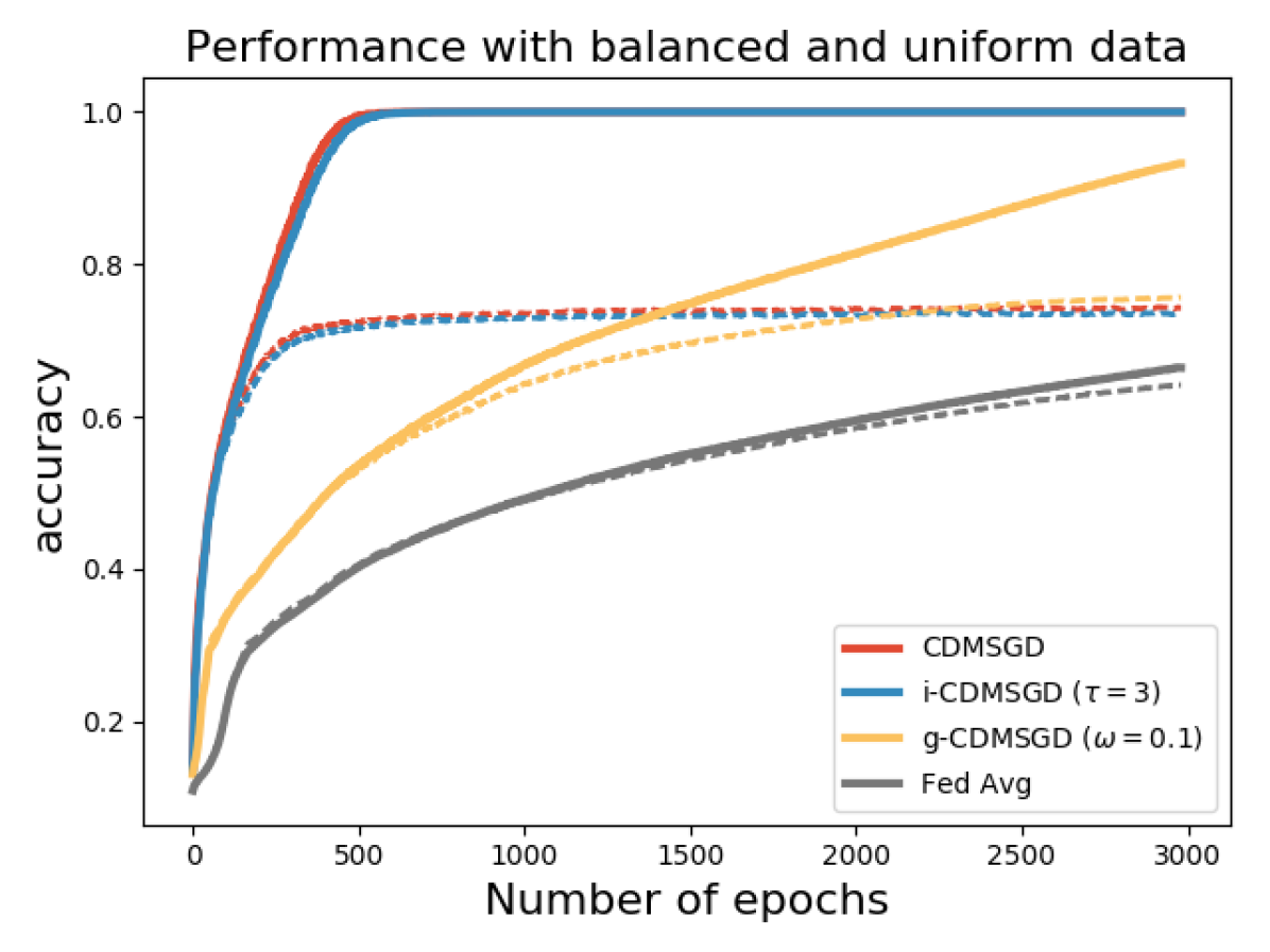
1:  Initialization: θ0j,v0j,j=1,2,,Nformulae-sequencesuperscriptsubscript𝜃0𝑗superscriptsubscript𝑣0𝑗𝑗12𝑁\theta_{0}^{j},v_{0}^{j},\;j=1,2,...,N, α𝛼\alpha, N𝑁N, τ𝜏\tau, m𝑚m, ΠΠ\Pi, μ𝜇\mu
2:  Distribute the Non-IID training data set to N𝑁N agents
3:  for each agent do
4:     Randomly shuffle each data subset
5:     for k=0:m:𝑘0𝑚k=0:m do
6:        t=0𝑡0t=0
7:        for j=1,,N𝑗1𝑁j=1,...,N do
8:           θtj=θkjsubscriptsuperscript𝜃𝑗𝑡subscriptsuperscript𝜃𝑗𝑘\theta^{j}_{t}=\theta^{j}_{k}
9:           vtj=vkjsubscriptsuperscript𝑣𝑗𝑡subscriptsuperscript𝑣𝑗𝑘v^{j}_{t}=v^{j}_{k}
10:        end for
11:        for j=1,,N𝑗1𝑁j=1,...,N do
12:           while tτ1𝑡𝜏1t\leq\tau-1 do
13:              θt+1j=lNb(j)πjlθtlsubscriptsuperscript𝜃𝑗𝑡1subscript𝑙𝑁𝑏𝑗subscript𝜋𝑗𝑙subscriptsuperscript𝜃𝑙𝑡\theta^{j}_{t+1}=\sum_{l\in Nb(j)}\pi_{jl}\theta^{l}_{t}
14:              vt+1j=lNb(j)πjlvtlsubscriptsuperscript𝑣𝑗𝑡1subscript𝑙𝑁𝑏𝑗subscript𝜋𝑗𝑙subscriptsuperscript𝑣𝑙𝑡v^{j}_{t+1}=\sum_{l\in Nb(j)}\pi_{jl}v^{l}_{t}{Momentum Consensus}
15:              t=t+1𝑡𝑡1t=t+1
16:           end while
17:        end for
18:        θ^=θtj^𝜃subscriptsuperscript𝜃𝑗𝑡\hat{\theta}=\theta^{j}_{t}
19:        v^=vtj^𝑣subscriptsuperscript𝑣𝑗𝑡\hat{v}=v^{j}_{t}
20:        vk+1j=θ^θkj+μv^αgj(θkj)superscriptsubscript𝑣𝑘1𝑗^𝜃subscriptsuperscript𝜃𝑗𝑘𝜇^𝑣𝛼subscript𝑔𝑗subscriptsuperscript𝜃𝑗𝑘v_{k+1}^{j}=\hat{\theta}-\theta^{j}_{k}+\mu\hat{v}-\alpha g_{j}(\theta^{j}_{k})
21:        θk+1j=θkj+vk+1jsubscriptsuperscript𝜃𝑗𝑘1subscriptsuperscript𝜃𝑗𝑘subscriptsuperscript𝑣𝑗𝑘1\theta^{j}_{k+1}=\theta^{j}_{k}+v^{j}_{k+1}
22:     end for
23:  end for
Algorithm 3 i-CDMSGD
1:  Initialization: ω𝜔\omega, θ0j,v0j,j=1,2,,Nformulae-sequencesuperscriptsubscript𝜃0𝑗superscriptsubscript𝑣0𝑗𝑗12𝑁\theta_{0}^{j},v_{0}^{j},\;j=1,2,...,N, α𝛼\alpha, N𝑁N, m𝑚m, ΠΠ\Pi, μ𝜇\mu
2:  Distribute the Non-IID training data set to N𝑁N agents
3:  for each agent do
4:     Randomly shuffle each data subset
5:     for k=0:m:𝑘0𝑚k=0:m do
6:        θ^=lNb(j)πjlθtl^𝜃subscript𝑙𝑁𝑏𝑗subscript𝜋𝑗𝑙subscriptsuperscript𝜃𝑙𝑡\hat{\theta}=\sum_{l\in Nb(j)}\pi_{jl}\theta^{l}_{t}
7:        v^=lNb(j)πjlvtl^𝑣subscript𝑙𝑁𝑏𝑗subscript𝜋𝑗𝑙subscriptsuperscript𝑣𝑙𝑡\hat{v}=\sum_{l\in Nb(j)}\pi_{jl}v^{l}_{t}
8:        vk+1j=(1ω)(θ^θkj+μv^)+ωμvkjωαgj(θkj+μvkj)superscriptsubscript𝑣𝑘1𝑗1𝜔^𝜃subscriptsuperscript𝜃𝑗𝑘𝜇^𝑣𝜔𝜇subscriptsuperscript𝑣𝑗𝑘𝜔𝛼subscript𝑔𝑗subscriptsuperscript𝜃𝑗𝑘𝜇subscriptsuperscript𝑣𝑗𝑘v_{k+1}^{j}=(1-\omega)(\hat{\theta}-\theta^{j}_{k}+\mu\hat{v})+\omega\mu v^{j}_{k}-\omega\alpha g_{j}(\theta^{j}_{k}+\mu v^{j}_{k})
9:        θk+1j=θkj+vk+1jsuperscriptsubscript𝜃𝑘1𝑗subscriptsuperscript𝜃𝑗𝑘subscriptsuperscript𝑣𝑗𝑘1\theta_{k+1}^{j}=\theta^{j}_{k}+v^{j}_{k+1}
10:     end for
11:  end for
Algorithm 4 g-CDMSGD
Refer to caption
(a) Performance of different algorithms on balanced and uniformly distributed data among agents. (Dashed lines represent test accuracy & solid lines represent training accuracy.)
Refer to caption
(b) Performance of different non-momentum versions of the algorithms. (Dashed lines represent test accuracy & solid lines represent training accuracy.)
Refer to caption
(c) Performance of g-CDMSGD algorithm with different ω𝜔\omega values with an unbalanced and non-uniform distribution of data (20% non uniformity).
Refer to caption
(d) Performance of g-CDMSGD algorithm with different ω𝜔\omega values with an unbalanced and non-uniform distribution of data (40% non uniformity).
Refer to caption
(e) Performance of g-CDMSGD algorithm with different ω𝜔\omega values with an unbalanced and non-uniform distribution of data (60% non uniformity).
Refer to caption
(f) Performance of different algorithms with a balanced data distribution on MNIST dataset
Figure 3: Results from numerical experiments on several data distributions for CIFAR10 and also one experiment on MNIST data set

A.4   Additional Experimental Results

In all our experiments. we consider the number of agents to be 5. We choose the following sparse agent interaction matrix for all our experiments.

π=[0.340.330.00.0.330.330.340.330.00.00.00.330.340.330.00.00.00.330.340.330.330.00.00.330.34]𝜋matrix0.340.330.000.330.330.340.330.00.00.00.330.340.330.00.00.00.330.340.330.330.00.00.330.34\pi=\begin{bmatrix}0.34&0.33&0.0&0.&0.33\\ 0.33&0.34&0.33&0.0&0.0\\ 0.0&0.33&0.34&0.33&0.0\\ 0.0&0.0&0.33&0.34&0.33\\ 0.33&0.0&0.0&0.33&0.34\\ \end{bmatrix}

More results are shown in Figure. 3. In Figure 3(a), we see that fluctuations in the average accuracy are almost negligible for the case where each agent gets balanced and uniformly distributed dataset. Algorithm i-CDMSGD performs as good as CDMSGD. We also notice that g-CDMSGD has a lower convergence rate but achieves slightly better test error which shows similar trend with Unbalanced data distribution case shown in Figure 2(a). Figure 3(b) shows the performance of the non-momentum versions of the same settings. Algorithms i-CDSGD and CDSGD perform similar to Federated Averaging whereas g-CDSGD is slow but the generalization gap is lesser.

For all the experiments until this point, each agent is allocated data from a uniform distribution of data (assured by shuffling of the data). However, it is possible that each agent can have non-uniformity in the distribution of data they are receiving. One of the aspect of non-uniformity is when each agent gets samples biased towards a few (not all) classes and gets very few samples of other classes. Note that this kind of distribution is referred as non-iid data distribution in Federated Averaging[15]. For simulating this, we allocate a portion of samples pertaining to a class to a specific agent and the other portion will be pooled, shuffled and distributed. Figure 3(c)3(e) represents the performance of different algorithms with different percentage of non-uniform distribution of data (percentage of data per class allocated without any shuffling). For Figure 3(c), we split 20% of data pertaining to two classes to an each agent. Thus, each agent has a bias of 30%absentpercent30\approx 30\% towards a class. In such a non-uniform distribution of data, the performance of each agent fluctuates a lot more than the other the uniform distribution of data. With several values of ω𝜔\omega we see that as the value of ω𝜔\omega increases, the performance is close to CDMSGD and is even slightly better than it. At the same time, as the percentage of non-uniformity is increased to 60%, we see that the increasing ω𝜔\omega deteriorates the performance. This can be corroborated with the increase in the agent level difference in the performance and lack of consensus as well as more emphasis on local gradient updates (ω=0.5𝜔0.5\omega=0.5). Since, the algorithms have not reached stability, we could not compute the degree of consensus among the agents.

Finally, we also compare our proposed algorithms to CDMSGD on another benchmark dataset - MNIST. The performance of the algorithms is shown in Figure 3(f) which follows similar trend as observed for CIFAR-10.