Theoretical compensation of static deformations of freeform multi mirror substrates

Abstract

Varying temperatures influence the figure errors of freeform metal mirrors by thermal expansion. Furthermore, different materials lead to thermo-elastic bending effects. The article presents a derivation of a compensation approach for general static loads. Utilizing perturbation theory this approach works for shape compensation of substrates which operate in various temperature environments. Verification is made using a finite element analysis which is further used to produce manufacturable CAD models. The remaining low spatial frequency errors are deterministically correctable using diamond turning or polishing techniques.
(120.4880) Optomechanics, (120.6810) Thermal effects, (260.3910) Metal optics, (120.4610) Optical fabrication, (220.1920) Diamond machining

I Introduction and Motivation

Metal optics for space and ground-based applications have been state of the art for several years Riedl:2001 ; Gardner:Mather:Clampin:others:2006 ; Steinkopf:Gebhardt:Scheiding:others:2008 ; Risse:Gebhardt:Damm:others:2008 ; Horst:Tromp:Haan:others:2008 ; Nijkerk:vanVenrooy:vanDoorn:others:2012 ; Kerridge:Hegglin:McConnell:others:2012 ; Peschel:Damm:Scheiding:others:2014 ; Beier:Hartung:Peschel:others:2014 ; Schuermann:Gaebler:Schlegel:others:2016 . Polishable coatings like X-ray amorphous electroless nickel-phosphorus (NiP) Qin:2011 ; Park:Lee:1988 ; Hur:Jeong:Lee:1990 ; Dini:1991 ; Syn:Dini:Taylor:others:1985 ; Hibbard:1997 ; Steinkopf:Gebhardt:Scheiding:others:2008 ; Pramanik:Neo:Rahman:others:2008 ; Carrigan:2011 ; Feigl:Perske:Pauer:others:2015 ; Gebhardt:Scheiding:Kinast:others:2011 ; Risse:Gebhardt:Damm:others:2008 ; Gebhardt:Kinast:Rohloff:others:2014 extend the range of applicable surface finishing methods to include chemical mechanical or computer controlled polishing (CMP, CCP) or Magnetorheological finishing (MRF) Steinkopf:Gebhardt:Scheiding:others:2008 ; Schuermann:Gaebler:Schlegel:others:2016 ; Carrigan:2011 ; Feigl:Perske:Pauer:others:2015 ; Gebhardt:Scheiding:Kinast:others:2011 ; Risse:Gebhardt:Damm:others:2008 ; Gebhardt:Kinast:Rohloff:others:2014 ; Kinast:Beier:Gebhardt:others:2015 and improve the achievable optical surface accuracy. There are several effects which lead to a change of the substrate shape (dimensional instability) and thus, of the optical surfaces. Dimensional instabilities are divided into three types: long-term, thermal cycling, and thermal Hibbard:1990 ; Folkman:Stevens:2002 ; Marschall:Maringer:1977 ; DeWitt:Eikenberry:Cardona:2008 ; Robichaud:Wang:Mastandrea:1998 ; Kinast:Grabowski:Gebhardt:others:2014 ; Vukobratovich:Gerzoff:Cho:1997 ; Moon:Cho:Richard:2003 ; Wang:Shouwang:Jinlong:others:2016 ; Zhou:Lin:Liu:others:2005 . Long-term instabilities are time dependent effects, like diffusion, phase transitions and stress relaxation of the materials used. Thermal cycling instabilities are plastic deformations due to thermal treatments. Different coefficients of thermal expansion (CTE) of the materials used lead to thermal instabilities. Dimensional instabilities lead in general to a non-acceptable degradation of the optical performance of the system which has to be restored by dimensional stable materials and one or more compensation approaches. Thermal instabilities can be compensated using kinematic means Yang:Liu:Wu:2012 ; Batteral:Fuss:Durieux:Martaut:2015 , active/adaptive optics Susini:Thomas:1993 ; Hubin:Noethe:1993 ; Reinlein:Appelfelder:Goy:others:2013 ; Goy:Reinlein:Devaney:others:2016 ; Reinlein:Brady:Damm:others:2016 ; Brady:Berlich:Leonhard:others:2017 , or compensation optics Krist:Burrows:1995 ; Slusher:Satter:Kaplan:others:1993 . While all aforementioned compensation approaches take place in a post-manufacturing stage or during the operation of the optical instrument, the subject of this article is compensation during manufacturing, possible when the static loads are known beforehand.

One important static effect is the isotropic linear thermal expansion or shrinkage of substrates made of one single material under certain temperature loads. For substrates coated with the previously mentioned polishing layer, non-linear and non-isotropic expansion and bending effects exist, too. To minimize these effects, the mismatch of the CTE between the typical substrate material aluminum (e.g. Al6061) and the NiP coating – which is responsible for the bending – has to be reduced. Therefore it is important to use a thermally matched material for the metallic substrate. In the case of NiP, 40 w% (weight percent) silicon-particle reinforced aluminum (designated as Al–40Si throughout the article) is considered, because the CTE mismatch between these materials is $<0.5\times 10^{-6}\,\text{K}^{-1}$ Hibbard:1995 ; Hibbard:1990 ; Kinast:Hilpert:Lange:others:2014 ; Kinast:Hilpert:Rohloff:others:2014 ; Rohloff:Gebhardt:Schoenherr:others:2010 .

Those effects lead to a specific surface form deviation (low spatial frequency contributions corresponding to figure errors), which reduces the performance of an optical system. In the case of a spherical mirror in a rotationally symmetric system, this performance degradation is predictable and correctable by adjusting the distances along the optical axis in this system, but for a freeform mirror the thermal expansion leads to an irregular surface form deviation, which cannot be compensated easily anymore. Additionally, if there is a polishing layer applied to this metal mirror substrate, the bimetallic bending effect induces a freeform deviation of the mirror surface, even for a relatively simple base shape. Even if the materials are thermally matched (small difference of their corresponding CTEs at the respective operational temperatures), the occuring small mismatch produces an undesirable bending effect at large differences between manufacturing temperature and the well-defined operation temperature. To predict and correct these thermo-elastic surface form deviations (thermal instability) of the optical surfaces before operation of the metal optics is the motivation of this paper.

Within this article, the calculations to quantify these effects and to perform a compensation are carried out for a metal two-mirror substrate which is part of a three-mirror-anastigmat (TMA). The two-mirror substrate consists of the primary mirror (M1) and the tertiary mirror (M3). It is made of Al–40Si and coated with NiP. Both mirrors M1 and M3 are aspheric with Zernike freeform contributions. For their manufacturing freeform techniques are necessary. The manufacturing and metrology usually take place at room temperature, but the operational environment is different. E.g., infrared (IR) optics are used at $-196\,{}^{\circ}$C to mitigate thermal noise effects. This specific temperature is chosen because it is achievable by using liquid nitrogen and denotes its boiling temperature. Although the mirror module is designed for the visual (VIS) spectral range, $-196\,{}^{\circ}$C in comparison to room temperature defines the temperature load case throughout the present article DeWitt:Eikenberry:Cardona:2008 ; Fuentes:Manescau:SanchezDeLaRosa:1994 ; Robinson:Huppi:Folkman:2002 ; Shen:Lin:Ma:others:1996 .

To describe the theory of thermo-elastic deformations, tensor calculus is necessary. All vectorial and tensorial calculations are carried out by utilizing a simplified Einsteinian summation convention, i.e. over double indices in one term is summed and the $\sum$ symbol is neglected (e.g. the matrix multiplication $C_{ij}=A_{ik}B_{kj}$ is short for $C_{ij}=\sum_{k=1}^{3}A_{ik}B_{kj}$). Further vector and tensor indices $i,j,k,\dots$ denoting their components are always from the middle of the Latin alphabet and their values are $1,\dots,3$. Different material indices $a,b,\dots$ are from the beginning of the Latin alphabet. In the following calculations, the vector field $\mathbf{u}(\mathbf{x})$ denotes the deformation of a single volume element in a macroscopic substrate at the field evaluation point $\mathbf{x}=(x_{i})=(x,y,z)^{T}$. The dependency of certain fields on the point $\mathbf{x}$ is mostly omitted within the formulas. Further $\sigma_{ij}~{}=~{}\sigma_{ji}$ is the stress tensor field and $\delta_{ij}$ the Kronecker delta, which is $1$ for $i=j$ and $0$ for $i\neq j$, respectively. $\partial_{i}$ denotes the partial derivative in the $i$-th direction. From the partial derivatives and the deformation field, the symmetrical infinitesimal geometrical linearized strain tensor $u_{ij}~{}=~{}\tfrac{1}{2}(\partial_{i}u_{j}~{}+~{}\partial_{j}u_{i})$ is composed. Since the strain tensor is derived from the length of an infinitesimal distance between two points in the substrate before and after deformation, its full form is given by $u_{ik}=\frac{1}{2}(\partial_{i}u_{k}+\partial_{k}u_{i}+\partial_{\ell}u_{i}\partial_{\ell}u_{k})$, where the last term is neglected throughout the article.

However, the optical design of the example system is decoupled from the present article. The optical analyses, e.g., footprint export, and coordinate systems analysis were performed by using the program ZEMAX ZEMAX:2017 . From ZEMAX, the surface exports need to be converted into a volume model. Therefore, the computer-aided design (CAD) program CREO Pro/Engineer ProE:2017 is used. The finite element analyses (FEA) are carried out by using ANSYS ANSYS:2017 and the data analysis steps were done utilizing the computer algebra system Mathematica Wolfram:1991 ; Wolfram:2003 .

There are three main tasks to be achieved within this article:

1. Theoretically derive general compensation formula to reduce optical influences of static load cases.

2. Simplify compensation formula for thermo-elastic load case.

3. Use finite element analyses to verify, apply, and compare different approaches for the derived compensation formula for the M1M3 metal mirror substrate including polishing coating for the aforementioned thermo-elastic load case.

Therefore, the present article is organized as follows. In section II the theoretical foundations of thermal effects in structural mechanics are described and the compensation formula is derived. To put the theoretical derivation into an application context, the TMA mirror system with the M1M3 mirror substrate and the corresponding manufacturing process chain are introduced in section III. The compensation formula as well as the model and manufacturing chain considerations are used in section IV to pre-deform a model and to perform an FEA to obtain the residual deformation for the thermal load case mentioned. There are also some consistency calculations presented. The article concludes with presentation of the results of the FEA in section V and shows a short outlook on the next steps in section VI.

II Theoretical Analysis

II.1 Elasticity Theory with Thermal Effects

From a theoretical point of view the top-down derivation starts by introduction of the total differential of the inner energy with a strain energy contribution for the deformation of a volume body,

$$\text{d}\mathcal{E} =T\text{d}S+\sigma_{ij}\text{d}u_{ij}\,.$$ (1)

From that, it is possible to use a Legendre transformation and turn the expression of the inner energy into one for the free energy,

$$\text{d}F =-S\text{d}T+\sigma_{ij}\text{d}u_{ij}\,.$$ (2)

This leads to a thermodynamic expression for the stress tensor in the isothermic case of constant temperature $T$ Landau:Lifshitz:6:1991 ,

$$\sigma_{ij} =\left(\frac{\partial F}{\partial u_{ij}}\right)_{T}\,.$$ (3)

To get an expression for the stress tensor, it is necessary to provide a concrete form of the free energy $F$ in dependence of the strain tensor $u_{ij}$. The most simple way to construct such an expression is to use a series expansion in $u_{ij}$, where the only appearing terms may be scalars built up from $u_{ij}$. It is further necessary that for $u_{ij}~{}=~{}0$ at constant temperature, the stress tensor vanishes, too. The expansion has to start at quadratic order in $u_{ij}$. If $F$ consists of quadratic parts in $u_{ij}$ only, the arising dependency between $\sigma_{ij}$ and $u_{ij}$ is linear and is called Hooke’s law.

Nevertheless, thermal expansion effects change the argumentation from above, since there is also a net deformation without exterior forces acting on the material. Therefore, the free energy of an isotropic single material deformable substrate for a small temperature range $\text{d}T$ starts at linear order in $u_{ij}$ and is given by

$$F(T) =F_{0}(T)-3K(T)\alpha(T)\text{d}T\;u_{\ell\ell}$$

$$+\mu(T)\;\left(u_{ik}-\frac{1}{3}\delta_{ik}u_{\ell\ell}\right)^{2}+\frac{K(T)}{2}\;u_{\ell\ell}^{2}\,,$$ (4)

where $\alpha(T)$ (CTE), $K(T)$ (compression modulus), $\mu(T)$ (shear modulus) are considered to be spatially constant but functions of the temperature. For the present article, the temperature ranges are not small and in addition, the CTE data is obtained from a push–rod dilatometer, which works by applying a constant force to a sample and monitors its length change during well-defined temperature variations. Therefore, in this measurement all temperature dependencies of the elastic moduli are cumulated in an effective temperature dependency of $\alpha(T)$ and hence, they are taken as being constant, $K(T)=\text{const}$ and $\mu(T)=\text{const}$. Considering a finite temperature range $T-T_{0}$ for the elastic substrate, the free energy contribution $\sim\alpha(T)\text{d}T$ has to be integrated over this range. Since the temperature difference $T-T_{0}$ is a constant throughout this article, it is useful to substitute the integral by an averaged CTE,

$$\bar{\alpha} =\frac{1}{T-T_{0}}\int_{T_{0}}^{T}\text{d}T\alpha(T)\,.$$ (5)

This leads to a modified free energy for a finite temperature difference $T-T_{0}$

$$F(T) =\bar{F}_{0}-3K\bar{\alpha}(T-T_{0})\;u_{\ell\ell}$$

$$+\mu\;\left(u_{ik}-\frac{1}{3}\delta_{ik}u_{\ell\ell}\right)^{2}+\frac{K}{2}\;u_{\ell\ell}^{2}\,.$$ (6)

From the free energy the stress tensor $\sigma_{ik}$ can be obtained by (3),

$$\sigma_{ik} =-3K\bar{\alpha}(T-T_{0})\delta_{ik}+K\;u_{\ell\ell}\delta_{ik}+2\mu\;\left(u_{ik}-\frac{1}{3}\delta_{ik}u_{\ell\ell}\right)\,.$$ (7)

The first term is the constant term due to linear contributions of $u_{\ell\ell}$ to the free energy. The second and third terms are the contraction and shear contributions to the stress tensor, respectively. As described in Landau:Lifshitz:6:1991 there may be no internal stresses in the material for a simple thermal expansion and therefore the stress tensor has to vanish,

$$\sigma_{ik} =0\,.$$ (8)

This relation is valid for all field evaluation points $\mathbf{x}$ within the substrate. (In the present article, $\alpha$ is the linear coefficient of thermal expansion, while in Landau:Lifshitz:6:1991 , the volume coefficient of thermal expansion is used. Further, the connection between shear modulus and contraction modulus on the one hand and Young’s modulus and Poisson number, which are typically used as material parameters, is $E~{}=~{}\frac{9K\mu}{3K+\mu}$ and $\nu~{}=~{}\frac{3K-2\mu}{6K+2\mu}$, respectively. If there are exterior forces acting on the substrate or stresses are induced, the full stationary equations of motion $-\partial_{i}\sigma_{ij}=f_{j}$ are to be solved.) As it is known from representation theory, the trace part and the symmetric trace free (STF) or shear part transform independently under the group of the orthogonal $3\times 3$ transformations with determinant one ($SO(3)$). Therefore, vanishing of the stress tensor leads to two conditions. From cancellation of the $\mu$ proportional STF part, it follows $u_{ik}=\text{const}\cdot\delta_{ik}$; from cancellation of the trace part, one obtains

$$u_{\ell\ell} =3\bar{\alpha}(T-T_{0})\,.$$ (9)

Therefore,

$$u_{ik} =\frac{1}{2}(\partial_{i}u_{k}+\partial_{k}u_{i})=\bar{\alpha}(T-T_{0})\delta_{ik}\,.$$ (10)

For $T-T_{0}=\text{const}$, one solution to this equation is

$$u_{k} =\bar{\alpha}(T-T_{0})x_{k}+u_{0\,k}+A_{km}x_{m}\,,$$ (11)

where $A_{km}=-A_{mk}$. In particular, this is valid for $A_{km}=\tfrac{1}{2}\varepsilon_{kjm}a_{0\,j}$. The last part contributes to the rotation of $\mathbf{u}(\mathbf{x})$ only, but does not affect the symmetrical derivative $u_{ik}$.

Usually, for the deformation field there is no requirement to be zero at all of the volume boundaries of the solid body under consideration. This would render the mechanical system over–constrained. Without any boundary conditions applied, the solution of (11) – in classical notation – is thus given by

$$\mathbf{u}(\mathbf{x}) =\bar{\alpha}(T-T_{0})\mathbf{x}+\mathbf{u}_{0}+\frac{1}{2}\mathbf{a}_{0}\times\mathbf{x}\,,$$ (12)

where $\mathbf{u}_{0}$ and $\mathbf{a}_{0}$ are integration constants.

Until now, the thermal expansion of a substrate containing only one material is described. Equation (12) shows that there are no bending effects as $\mathbf{u}$ depends only linearly on $\mathbf{x}$ only. If there are two materials present (e.g. NiP coated Al–40Si), the situation changes. Their different CTEs lead to different expansions and thus, stresses at the contact boundary and a bending of both occur. For two metal stripes bonded together with a respective thickness of $t_{a}$, Young’s moduli of $E_{a}$, and averaged CTEs $\bar{\alpha}_{a}$ ($a=1,2$), the analytical description of their curvature is given by

$$\frac{1}{R} =\frac{6(\bar{\alpha}_{1}-\bar{\alpha}_{2})(T-T_{0})\left(1+\tau\right)^{2}}{(t_{1}+t_{2})\left[3\left(1+\tau\right)^{2}+\left(1+\tau\varepsilon\right)\left(\tau^{2}+\frac{1}{\tau\varepsilon}\right)\right]}\,,$$ (13)

where $\tau~{}=~{}t_{1}/t_{2}$ is the thickness ratio and $\varepsilon~{}=~{}E_{1}/E_{2}$ is Young’s modulus ratio Timoshenko:1925 . There also exist several generalizations of (13) for, e.g., multi material stripes. The deflection for a substrate of length $L$ fixed in $z$ direction on both ends is approximately derived from the geometrical relation

$$\Delta z =R\left(1-\sqrt{1-\frac{L^{2}}{4R^{2}}}\right)\,,$$ (14)

which is shown in fig. 1. The stripe is fixed in $z$ direction, but in $x$ direction it is only fixed on the left hand side. Since the substrate length is mostly much smaller than the curvature radius $R$, one may use a second order approximation in $L/(2R)\ll 1$,

$$\Delta z \approx\frac{L^{2}}{8R}\,.$$ (15)

In contrast for a one sided fixed stripe, which is free on the other side, the $z$ deformation is given by $\Delta z\approx\frac{L^{2}}{2R}$.

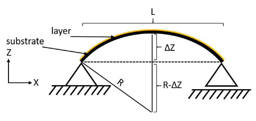
Figure 1: Principle of bimetallic bending effect

Assuming that the corresponding deformation field $\mathbf{u}(\mathbf{x})$ is mostly dominated by $u_{z}(x,0,z)$ and the strip is fixed in $z$ direction at both sides, $u_{z}(0,0,z)=0$, $u_{z}(L,0,z)=0$ and $u_{z}(L/2,0,z)=L^{2}/(8R)$, which leads in quadratic approximation to

$$\mathbf{u}_{\text{quadratic}}(x,0,z) \approx-\frac{1}{2R}\left[\left(x-\frac{L}{2}\right)^{2}-\frac{L^{2}}{4}\right]\mathbf{e}_{z}\,,$$ (16)

where $1/R$ from (13) is proportional to $T-T_{0}$ and the averaged CTE mismatch $\bar{\alpha}_{1}-\bar{\alpha}_{2}$.

Although the formulas given in the last paragraphs are correct in the most simple cases only (i.e. no gradients for the thermal expansion and metal stripe for the bending effects), they give an impression about the order of magnitude of certain effects ($\sim\bar{\alpha}(T-T_{0})$ for thermal expansion and $\sim(\bar{\alpha}_{1}-\bar{\alpha}_{2})(T-T_{0})$ for the bending) and provide a reason for dividing the deformation field $\mathbf{u}(\mathbf{x})$ the way it will be done in the following sections. Further, the M1M3 metal mirror substrate is neither a simple block of material nor a metal stripe, but the formulas derived above lead to certain consistency checks verifying the FEA in section IV.

II.2 Deformation Compensation

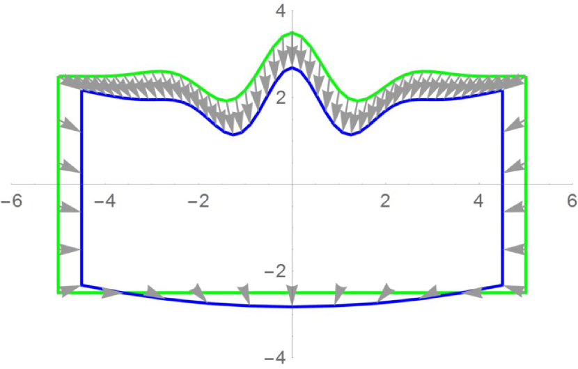
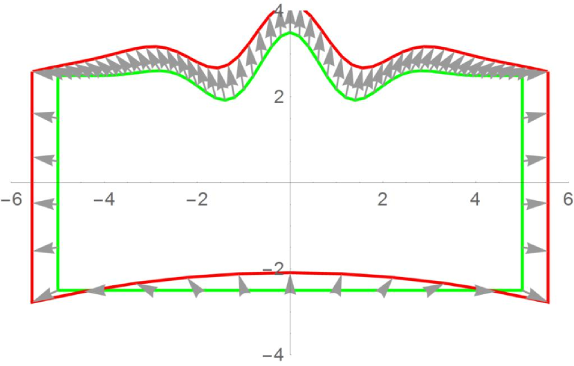
Figure 2: (a) Obtained cooling deformation. Green shows ideal substrate basis. Blue shows the deformed substrate after cooling.

(b) Calculated cooling compensating “heating” deformation (red) and pre-deformed substrate such that its form corresponds to the red line.

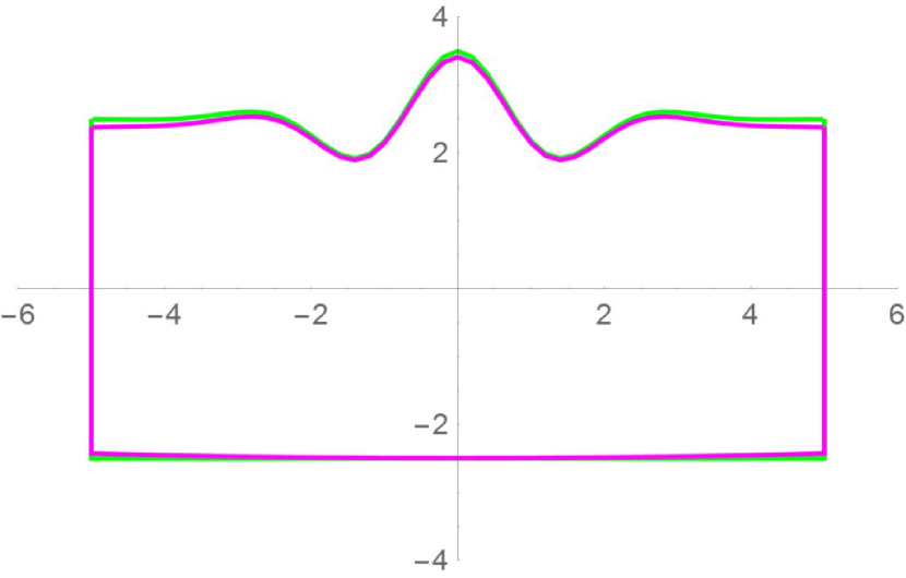
(c) Cooling of pre-deformed (red) substrate should give a small residual deformation compared to the original (violet).

The results of subsection II.1 show that for the material combinations considered in the present article, thermal expansion effects are much larger than thermal bending effects and therefore, $\mathbf{u}(\mathbf{x})$ is mostly affine linear with a small non-linear correction, namely

$$u_{i} =D_{ij}x_{j}+b_{i}+u_{i\,\text{nl}}(x_{k})\,.$$ (17)

The reason is, in (12) the field evaluation point $\mathbf{x}$ occurs in a linear manner only and in, e.g., (16) quadratic terms appear. The affine linear structure of the first two terms in (17) is chosen, because a certain mounting of the M1M3 mirror module throughout the FEA may produce residual linear contributions in $\mathbf{u}(\mathbf{x})$, which cannot be modelled by a simple divergence. To be able to extract those mounting effects, the full linear dependence is obtained by using a fit, whereas the CTE is given by the divergence of the linear part of the vector field (divergence parts coming from the non-linear correction are neglected),

$$\bar{\alpha}(T-T_{0}) =\frac{1}{3}D_{ii}\,,$$ (18)

and thus, by the trace of the matrix $D_{ij}$. Besides, the rotation of the vector field can be expressed by the matrix components,

$$(\text{rot}\,\mathbf{u})_{i} =\varepsilon_{ijk}\partial_{j}u_{k}=\varepsilon_{ijk}D_{jk}=a_{0\,i}\,.$$ (19)

The residual components are the symmetric traceless components of the matrix $D_{ij}$. These correspond to pure shearing of the material. By analysis of the different linear parts and subtracting them from the deformation field, the purely non-linear deformations are obtained. Therefore different parts of the deformation are well-defined and can easily be extracted from the fit data.

For a general derivation of the compensation procedure, a non-restricted $\mathbf{u}(\mathbf{x})$ is considered. The different steps of the compensation procedure are shown in fig. 2. These steps are shown more explicitly throughout the next paragraph. In this context, the article refers to cooling for the load case and heating for a virtual load case compensating the deformation of the former one.

When a substrate is being cooled down during a finite element analysis from $T_{0}$ to operation temperature $T<T_{0}$ (see fig. 2(a)) its new nodal positions are given by

$$\mathbf{x}_{c} =\mathbf{x}+\mathbf{u}_{c}(\mathbf{x})\,,$$ (20)

where $\mathbf{x}$ corresponds to the original nodal positions and $\mathbf{u}_{c}(\mathbf{x})$ is the deformation known according to the simulation. To compensate the known cooling deformation after applying the former load case it is necessary to deform the substrate before. The deformation could be considered as a “heating” from operation temperature $T$ to $T_{0}$, see fig. 2(b). Its corresponding nodal deformation is denoted by

$$\mathbf{x}_{w} =\mathbf{x}+\mathbf{u}_{w}(\mathbf{x})\,,$$ (21)

where $\mathbf{u}_{w}(\mathbf{x})$ is still unknown. The determination of $\mathbf{u}_{w}(\mathbf{x})$ for a known $\mathbf{u}_{c}(\mathbf{x})$ is the first goal of the present article. Afterwards, the compensated substrate (pre-deformed by $\mathbf{u}_{w}$) is cooled down with the load case leading to $\mathbf{u}_{c}$ and deformed nodal positions should end up near the ideal starting nodal positions $\mathbf{x}$, see fig. 2(c). In the following calculations, these considerations are formulated in a formal manner and a compensation equation is derived. This means

$$\mathbf{x} \stackrel{{\scriptstyle!}}{{=}}\mathbf{x}_{w}+\mathbf{u}_{c}(\mathbf{x}_{w})=\mathbf{x}+\mathbf{u}_{w}(\mathbf{x})+\mathbf{u}_{c}(\mathbf{x}+\mathbf{u}_{w}(\mathbf{x}))\,.$$ (22)

Cancellation of $\mathbf{x}$ leads to

$$\boxed{\mathbf{u}_{w}(\mathbf{x})+\mathbf{u}_{c}(\mathbf{x}+\mathbf{u}_{w}(\mathbf{x}))\stackrel{{\scriptstyle!}}{{=}}0}\,,$$ (23)

which is the compensation equation, where $\mathbf{u}_{c}$ is known and $\mathbf{u}_{w}$ should be calculated. Depending on the structure of $\mathbf{u}_{c}(\mathbf{x})$, this equation can be inverted analytically (e.g. for the purely linear case) or perturbatively (e.g. for a possible decomposition of $\mathbf{u}_{c}$ in some small and dominating part) or only numerically (for a general structure of $\mathbf{u}_{c}(\mathbf{x})$).

Since the thermal load case is dominated by linear deformations,

$$\mathbf{u}_{c} =D\mathbf{x}+\mathbf{b}\,,$$ (24)

(23) can be solved exactly by

$$\mathbf{u}_{w\,\text{lin}} =-(\mathds{1}+D)^{-1}(D\mathbf{x}+\mathbf{b})\,.$$ (25)

For performing a first order Taylor expansion in the non-linear correction, it is necessary to introduce a bookkeeping parameter $\beta$. The perturbative treatment is valid, because the non-linear correction is small compared to the linear part for thermal deformation problems. This leads to a correction of (24) which is determined by a higher order polynomial fit

$$\mathbf{u}_{c}(\mathbf{x}) =D\mathbf{x}+\mathbf{b}+\beta\mathbf{u}_{c\,\text{nl}}(\mathbf{x})\,.$$ (26)

Besides, the compensation field $\mathbf{u}_{w}=\mathbf{u}_{w\,\text{lin}}+\beta\mathbf{u}_{w\,\text{nl}}$ is divided into a linear and non-linear part. After inserting these two splittings into (23), a lengthy expression arises:

$$\mathbf{u}_{w\,\text{lin}}(\mathbf{x})+D\mathbf{x}+D\mathbf{u}_{w\,\text{lin}}(\mathbf{x})+\mathbf{b}$$

$$+\beta[\mathbf{u}_{w\,\text{nl}}(\mathbf{x})+D\mathbf{u}_{w\,\text{nl}}(\mathbf{x})$$

$$\quad+\mathbf{u}_{c\,\text{nl}}(\mathbf{x}+\mathbf{u}_{w\,\text{lin}}(\mathbf{x})+\beta\mathbf{u}_{w\,\text{nl}}(\mathbf{x}))]\stackrel{{\scriptstyle!}}{{=}}0\,.$$ (27)

In the Taylor expansion around $\beta=0$, all terms higher than linear order in $\beta$ have to be neglected to be consistent in the approximation. By setting $\beta=0$, the purely linear part (see (25) and (24)) is restored. All other orders in $\beta$ are calculated by sorting the Taylor expansion of (27) by powers of $\beta$ and setting them to zero term by term. Therefore, the leading order $\beta$ non-linear contribution of the compensation field is given by

$$\mathbf{u}_{w\,\text{nl}}(\mathbf{x}) =-(\mathds{1}+D)^{-1}\mathbf{u}_{c\,\text{nl}}((\mathds{1}+D)^{-1}(\mathbf{x}-\mathbf{b}))\,,$$ (28)

and the whole compensation field including the linear part by

$$\mathbf{u}_{w}(\mathbf{x}) \approx-(\mathds{1}+D)^{-1}\left[D\mathbf{x}+\mathbf{b}+\mathbf{u}_{c\,\text{nl}}((\mathds{1}+D)^{-1}(\mathbf{x}-\mathbf{b}))\right]\,.$$ (29)

The field $\mathbf{u}_{w}(\mathbf{x})$ shown in (29) is referred as “compensation” deformation field. It is a first order approximation to compensate a given $\mathbf{u}_{c}(\mathbf{x})$, if it can be decomposed into a dominant linear and a small non-linear part. In the following section, the example substrate M1M3 will be introduced and afterwards, the result (29) will be applied to the $-196\,{}^{\circ}$C load case within finite element analysis.

III Example System and Process Chain

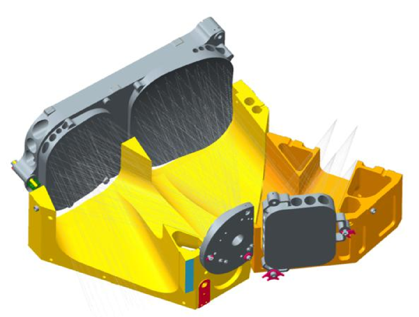
Figure 3: CAD model of the TMA with mirror substrates (grey) including housing (yellow).

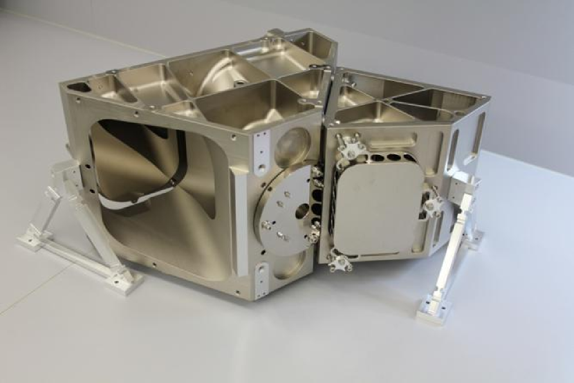
Figure 4: TMA after manufacturing and integration. The bipods shown in the picture are necessary to decouple the system from the mounting plate.

III.1 Optical Design Description of the TMA

The optical system is a TMA (see fig. 4 and fig. 4) consisting of three freeform mirrors and one folding mirror. Except the folding mirror, the mirrors M1, M2, and M3 (see tab. 2) are referenced to a single axis and only their $z$ position differs, see tab. 1 and fig. 5 respectively. Since M1 and M3 should be manufactured on one substrate their respective optical coordinate system is also located at a coincident position with the same axis orientations. The manufacturing coordinate system is then given by the fulfillment of the manufacturing constraints. It is tilted and decentered in relation to the optical coordinate system. The surface M2 is located at the system stop. The entrance pupil has a diameter of $81.25$ mm. Since the TMA is a telescope demonstrator, the object plane is located at infinity. This means, each raybundle for different points of the field of view (FOV) comes into the entrance pupil in different angles, but in a parallel manner. The FOV ranges between $-6.8^{\circ}$ and $6.8^{\circ}$ in $x$ direction and between $0^{\circ}$ and $6.3^{\circ}$ in $y$ direction. Further, there is a focal plane array (FPA) located at the image plane. Since keystone and smile distortion are typically specified for spectrometers they are also optimization criteria during the design process of this space technology demonstrator: its overall distortion magnitude is about $-2.94~{}\%$.

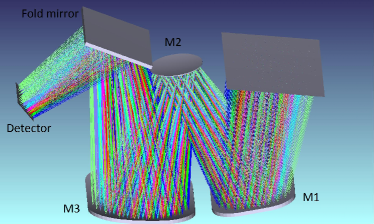
Figure 5: 3D optical design layout.

Table 1: Optical design for the TMA mirror system. (Thickness $t$, decenter in $Y$ direction $DY$, tilt angle $RX$ around $X$ axis, clear aperture CA.)

Surface	$t$ [mm]	$DY$ [mm]	$RX$ [∘]	CA [mm2]
Object	$\infty$	0	0	–
Entrance ap.	23	0	0	$109\times 74.5$
Coord. Break	0	0	$13.5$	–
M1	$-220$	0	0	user defined
M2	$220$	0	0	radius $40.5$
M3	$-230$	0	0	user defined
Coord. Break	0	0	$-30$	–
Fold mirror	0	0	0	$68.5\times 54.5$
Coord. Break	$220$	0	$-30$	–
Coord. Break	$-30$	$88.6$	0	–
Front surf. FPA	$30$	0	0	radius $100$
Detector	0	0	0	$40\times 20$

Table 2: Optical design data for the mirrors of the TMA. The Zernike contributions were neglected. Both vertex coordinate systems of M1 and M3 share a common point. The manufacturing coordinate system (i.e. the center for the diamond turning, see subsection III.3) is decentered and tilted vs. the optical coordinate system of the two vertices. The decenter in $y$ direction is $-15$ mm and the tilt around the $x$ axis is $-2.5^{\circ}$. (RoC $=$ radius of curvature, CC $=$ conic constant.)

Mirror	M1	M2	M3
RoC [mm]	$-1750.000$	$-401.923$	$-465.322$
CC [1]	$-69.850$	$27.909$	$-0.544$
A4 [mm-3]	$-3.422\times 10^{-10}$	$3.571\times 10^{-7}$	$-1.067\times 10^{-9}$
A6 [mm-5]	$1.833\times 10^{-14}$	$-3.836\times 10^{-10}$	$-3.351\times 10^{-15}$
A8 [mm-7]	$-7.748\times 10^{-20}$	$6.820\times 10^{-16}$	$-2.851\times 10^{-20}$
Freeform	Zernike Noll	Zernike Noll	Zernike Noll

III.2 Mechanical Design Description M1M3 Mirror Substrate

The STEP surface export from ZEMAX is taken as a starting point for generating a volume CAD model of the different mirror substrates. There are three different mirror substrates: the M1M3 substrate, the M2 substrate, and the fold mirror substrate. Due to its complicated structure and to demonstrate the general usability of the algorithms developed, the M1M3 substrate is considered as a demonstrator throughout this article. It does not have symmetries anymore, except the $YZ$ plane. The mirror surfaces are aspheric with Zernike freeform contributions. Due to the deviation of the manufacturing coordinate system from the optical coordinate system, manufacturing requires freeform techniques, even for spherical symmetric surface shapes. In this case, the compensation introduces also a freeform deviation from the optical design surface in general.

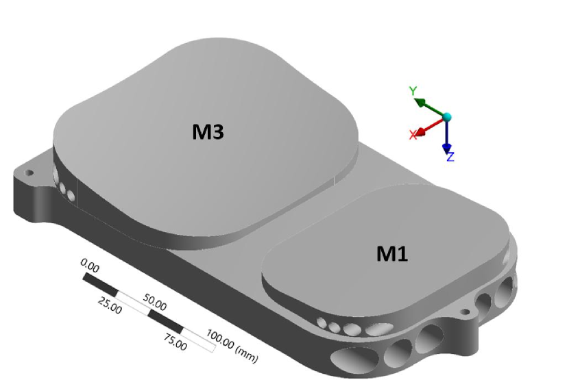
Figure 6: CAD model of the mirror substrate. The bounding box of this model is $205\,\text{mm}\times 339.5\,\text{mm}\times 60\,\text{mm}$. The mass of the model manufactured from Al–40Si with $100\,\upmu$m NiP polishing coating is $4.06$ kg. $100\,\upmu$m NiP polishing coating thickness is chosen to have enough material for the iterative UP diamond turning steps.

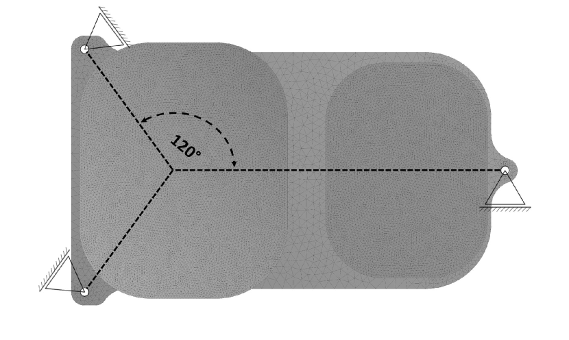
Figure 7: Isostatic mount points with an 120^∘ degree angle. The radial degree of freedom at the mountings is free, the tangential ones are fixed. The mesh elements are shown in color which represents the element quality, i. e. the aspect ratio.

III.3 Overview Manufacturing Process Chain

The first step of manufacturing is an artificial aging of the rough part to minimize thermal cycling instabilities and to achieve a long-term stable material behavior. Afterwards, the rough geometry of the substrate is obtained by a CNC manufacturing step, which is performed by a five-axis milling machine. Lightweight structures like crosswise bore holes are typically drilled or electrical discharge machined. These steps depend on a ready-to-use CAD model, which needs to satisfy certain conditions to be manufacturable. Therefore, it is necessary to discuss possibilities to obtain a mostly simplified CAD model, see subsection IV.2.2.

In the following, ultra-precise (UP) refers to an achievable figure error, which is in the micron range depending on the substrate size, its deviation from rotational symmetry, its material, and several other parameters. For the UP manufacturing step, the following main processes are available among others:

1. Ultra-precise diamond turning for which a substrate is mounted on the turning machine ($C$-) axis and a fixed tool is moved in a defined manner in $X$ and $Z$ direction to maintain the surface form. For a freeform manufacturing using the slow tool servo, the $Z$ axis is controlled in dependency of the $C$ values. For a higher dynamics of the freeform part, a fast tool servo is utilized, which introduces an additional voice coil driven $W$ axis. This axis has a lower maximal stroke than the whole $Z$ axis, but is more dynamical. It can only be used if the freeform part is not dominating the rotational symmetric part. For an imaging optical system, it is mostly possible to achieve this, see fig. 9 and fig. 9, Beier:Hartung:Peschel:others:2014 ; Scheiding:Damm:Holota:others:2010 ; Risse:Scheiding:Gebhardt:others:2011 .

2. Milling is necessary if the rotational symmetry of a part is broken strongly. It typically lasts longer than diamond turning processes. But $C$ axis milling in combination with diamond turning is also useful to provide references for tactile or interferometric metrology onto a metal mirror substrate. This is necessary to utilize the snap-together approach Beier:Hartung:Peschel:others:2014 .

A typical post-processing step to maintain a figure error down to $20$ nm r.m.s (root-mean-square). and around $1$ nm r.m.s. surface microroughness is the MRF step, where a fluid on a wheel and a magnetic field is used to generate a well-defined abrasive behaviour by controlling the dwell-time of the polishing wheel on the NiP coated substrate.

Figure 8: Freeform toolpath for fast tool servo with continuous toolpath between mirror surfaces M1 and M3.

Figure 9: Tool acceleration for fast tool servo on a decadic logarithmic scale in units of $g=9.81\,\text{m}/\text{s}^{2}$.

IV Finite Element Analysis

IV.1 Model and Materials

Table 3: Material data. The CTE mismatch is $0.5\times 10^{-6}\text{K}^{-1}$.

Name	Al–40Si	NiP
Young’s modulus [MPa]	102000	170000
Poisson number [1]	0.27	0.27
CTE [K${}^{-1}\times 10^{-6}$] @ 20 ∘C	13.0	12.5

The finite element model of the mirror substrate derived from the CAD model is built with 10-nodes tetrahedron (Solid187) elements for the substrate and 4-nodes quad (Shell181) elements for the NiP coating (see tab. 3 for the material data). Both elements have coincident nodes at the contact area. Shell elements for modelling the NiP coating are necessary, since for a sufficient mesh quality the aspect ratio of the linear dimensions of the volume elements should be of order one. This is violated for thin surface elements. (Since the thickness of the surface elements is approximately $100\,\upmu$m and their lateral dimensions are around $3\,$mm, they can be considered as thin.) Therefore, such coatings are usually modelled by using shell elements.

Based on the mounting concept for metallic mirrors, an isostatic mounting (ISM) is used for the boundary conditions model. Therefore, only the out-of-plane and the tangential component of the in-plane degrees of freedom (DOF) are appended to three bearings, which have a symmetrical $120^{\circ}$ grid arrangement, see fig. 7. For this reason, a rigid body element (RBE3, not infinitely stiff) is attached at each of the three bores of the mirror substrate. This does not increase the stiffness of the model. The reference nodes (pilot node in ANSYS) of the RBE3 boundary condition are constrained in the tangential $\phi$ and $z$ DOFs with respect to a cylindrical coordinate system. In contrast, the radial $r$ DOF of every RBE3 element is free in the mentioned cylindrical coordinate system. Therefore, the ISM generates a statically determined low-stress coupling with regard to thermal expansion.

A thermal condition is applied for both the mirror substrate body and the layer shells. Each of the elements composing the substrate and the coating are set to a specific temperature $T\neq T_{0}$, justifying usage of (9) and (17) for modelling the $\mathbf{u}$ field without any NiP layer (e.g. Al6061 or Al–40Si only). For the model with NiP layer, there are stresses induced at the boundary of the substrate due to different CTEs and hence, non-linear corrections to (17) have to be taken into account, see (29).

Modelling the $\mathbf{u}$ field in this context means that after FEA, a global fit of the deformation field over the model is carried out by using (17). From there, the compensation field is determined and put into another FEA with the same load cases. This leads to a net deformation on the mirror surfaces, which are compared to the optical design afterwards. Notice that a fit in general violates the boundary conditions of the FEA and therefore the compensation field does not satisfy any well-defined boundary conditions, too. However, this is acceptable, since it is only used for deformation of the base geometry.

IV.2 Simulations

Figure 10: Data flow for exact compensation within the ANSYS FEA software. The load case is given by a temperature ramp starting at $22\,{}^{\circ}$C and ending at $-196\,{}^{\circ}$C.

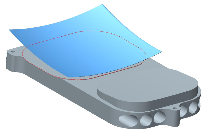
Figure 11: Compensation of the CAD model of the mirror substrate by generating the necessary exact compensated surfaces and increasing the size of the substrate isotropically.

IV.2.1 Dataflow Exact Compensation

In the “exact” compensation, the field $\mathbf{u}_{w}$, see (29), is used to displace the nodal positions in the whole model. As far as the deformation field has a smaller magnitude than the size of the elements, it does not lead to any problems like breaking of elements. During mechanical design stage (see subsection III.2) a CAD model is created to perform the CNC manufacturing, and also for the documentation of every step in the process chain. It is necessary to maintain the connection of the FEA model (mesh together with boundary conditions) to the CAD model after the compensation as well. By the calculated nodal deformation of the whole model, this connection is lost. Another major drawback is that edges may not be straight anymore or plane surfaces may also be deformed. Therefore, the exact compensation of all nodal position is of theoretical interest, but does not satisfy certain constraints, which are necessary for manufacturing.

IV.2.2 Dataflow CAD-based Compensation

Thus, a reduced compensation is performed. Starting from the fully deformed model, the necessary exact surface deviation is extracted. This is used to modify the former ideal surfaces. But for the volume model only an isotropic expansion is performed by using the effective CTE extracted from the $D_{ij}$ matrix fit. This leads to straight lines and surfaces after the deformation and therefore, they are still usable for mounting and clamping purposes on the machines. In fig. 11, building the CAD conform model is shown. Exactly deformed surfaces are created by using spline patches, which were generated from the compensated nodal positions on the surface. Those spline patches are used as a boundary surface for the extrusion of the surface footprints from the main substrate after its isotropic expansion.

In the following section, the resulting figure error after cooling the compensated geometry is compared for these two approaches.

V Results

During temperature change, each metal undergoes a certain thermal expansion. This thermal expansion is isotropic and linear for a single isotropic material and is non-isotropic and non-linear for a group of bonded different materials. For the case of metal mirror substrates, both effects lead to a deviation of the optical surface shapes from the intended design form. Throughout the present article, those effects were discussed for a metal mirror substrate with two mirrors, which is part of a TMA introduced in section III. The double mirror substrate and the thermal load case are both examples to demonstrate the feasiblity of the general compensation approach developed in subsection II.2 to compensate the deviations mentioned above. This approach relies on the precise knowledge of the temperature load, which arises between manufacturing process and operational environment of the optical component.

Given the compensation formula (23), there were two algorithms developed to change the substrate in such a manner that a further application of the temperature load leads to a net surface contribution, which is far smaller than without compensation. Although (23) is exact and quite general, the decomposition of the thermal load in this article into a large expansion part and a small bending part allows to find a closed form first order perturbative compensation formula for the necessary deformation of the original substrate, see (29).

The exact compensation leads to a non-manufacturable geometry of the part, because, e.g., straight lined lightweight structures get bended in general. This approach (see subsection IV.2.1) is not feasible for production. For the thermal load case, the deformations may be divided into a large linear and a small non-linear bending part. Therefore, it is also possible to produce a CAD model with the desired compensation properties, which is also manufacturable in the CNC fabrication step before ultra-precise diamond turning (see subsection IV.2.2). Further, the $z$ value compensation of the optical surfaces is in a range, which is also tractable by diamond turning techniques. Therefore, the developed compensation approaches are in-situ and fit into an existing manufacturing chain for metal mirrors right before the finishing process steps.

In the following, the optical surface deviations from design are illustrated and compared between the uncompensated model, the exact nodal compensation approach and the CAD compensation one.

Figure 12: M1 after cooling, uncompensated. Form deviation p.-v. $\approx~{}{21.8}$ $\mu$m, r.m.s. $\approx{5.8}$ $\mu$m.

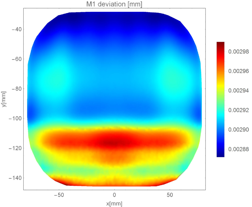
Figure 13: M1 after cooling, exactly compensated. Form deviation p.-v. $\approx~{}{118}$ nm, r.m.s. $\approx{26}$ nm.

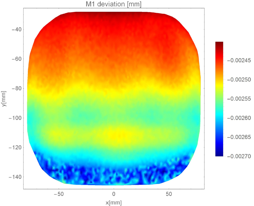
Figure 14: M1 after cooling, CAD compensated. Form deviation p.-v. $\approx~{}{301}$ nm, r.m.s. $\approx{61}$ nm. PST/TIP/TLT: $-2.37\,\upmu$m/$0^{\circ}$/$0.37^{\prime\prime}$, after removal
p.-v./r.m.s.: 166 nm/19 nm

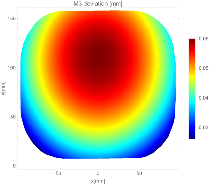
Figure 15: M3 after cooling, uncompensated. Form deviation p.-v. $\approx~{}{34.4}$ $\mu$m, r.m.s. $\approx{8.6}$ $\mu$m.

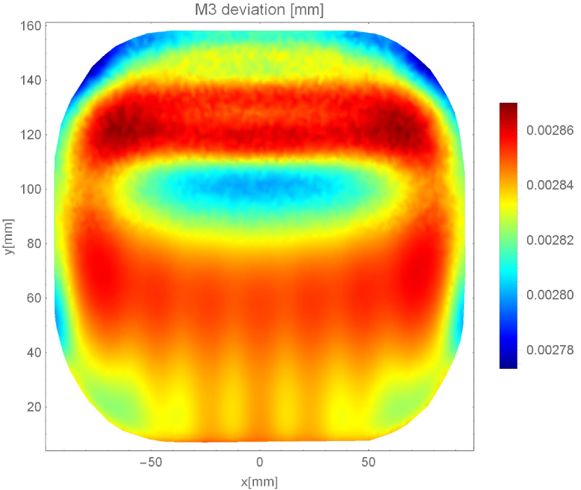
Figure 16: M3 after cooling, exactly compensated. Form deviation p.-v. $\approx~{}{97}$ nm, r.m.s. $\approx{16}$ nm.

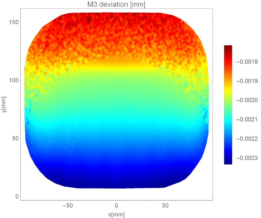
Figure 17: M3 after cooling, CAD compensated. Form deviation p.-v. $\approx~{}{618}$ nm, r.m.s. $\approx{160}$ nm. PST/TIP/TLT: $-2.36\,\upmu$m/$0^{\circ}$/$0.79^{\prime\prime}$, after removal
p.-v./r.m.s.: 171 nm/21 nm

The FEA results show that the thermal deformation due to the cooling of a highly asymmetric Al–40Si mirror substrate with a NiP layer from room temperature down to $-196\,{}^{\circ}$C may be compensated within two approaches. Those are also able to achieve a low figure error for the CAD compensated and for the exactly compensated model. The usual form deviation for the thermally matched material combination without any compensation in this temperature range is of several microns for M1 and M3, respectively. Therefore, the compensation approach may be used to increase performance significantly for freeform mirrors that are not manufactured at operation temperature, for non-thermally matched mirror substrates with their respective polishing coatings, or even for substrate materials that are both thermally matched.

VI Summary and Outlook

The magnitude of the compensation in case of thermal loads is of an order accessible by diamond turning or other ultra-precise manufacturing steps. But even if the temperature loads are small, the order of magnitude is due to its mainly low spatial frequency content still accessible by MRF figure correction. It is emphasized that cryogenic thermal loads discussed throughout the present article are an example for well-defined pre-compensable static loads. Although the compensation approach is usable for substrates, which operate in, e.g., a high-temperature environment. The general formula (23) does not make assumptions about the type of deformation.

In the future the experimental verification of the derived compensation approach has to be carried out. The present article contains theoretical considerations and the verification of the compensation was only done by FEA. Next step is to manufacture a compensated substrate and perform the appropriate figure measurements by interferometric techniques under cryogenic conditions.

VII Acknowledgements

The authors thank Matthias Beier, Andreas Gebhardt, Thomas Peschel, and Stefan Risse for very useful and enlighting discussions. Further they thank Stephanie Hesse-Ertelt and Aoife Brady for helpful corrections. This work is partly funded by Federal Ministry of Education and Research (BMBF) within framework “Unternehmen Region – Innovative Regional Growth Core” grant number 03WKCK1B.

References

- (1) M. J. Riedl, Optical Design Fundamentals for Infrared Systems. Spie Press, 2nd ed., 2001.
- (2) J. P. Gardner, J. C. Mather, M. Clampin, R. Doyon, M. A. Greenhouse, H. B. Hammel, J. B. Hutchings, P. Jakobsen, S. J. Lilly, K. S. Long, J. I. Lunine, M. J. McCaughrean, M. Mountain, J. Nella, G. H. Rieke, M. J. Rieke, H.-W. Rix, E. P. Smith, G. Sonneborn, M. Stiavelli, H. S. Stockman, R. A. Windhorst, and G. S. Wright, “The James Webb Space Telescope,” Space Sci. Rev. 123 (2006) 485–606, arXiv:astro-ph/0606175.
- (3) R. Steinkopf, A. Gebhardt, S. Scheiding, M. Rohde, O. Stenzel, S. Gliech, V. Giggel, H. Löscher, G. Ullrich, P. Rucks, A. Duparré, S. Risse, R. Eberhardt, and A. Tünnermann, “Metal mirrors with excellent figure and roughness,” Proc. SPIE 7102 (2008) 71020C.
- (4) S. Risse, A. Gebhardt, C. Damm, T. Peschel, W. Stöckl, T. Feigl, S. Kirschstein, R. Eberhardt, N. Kaiser, and A. Tünnermann, “Novel tma telescope based on ultra precise metal mirrors,” Proc. SPIE 7010 (2008) 701016.
- (5) R. ter Horst, N. Tromp, M. de Haan, R. Navarro, L. Venema, and J. Pragt, “Directly polished lightweight aluminum mirror,” Proc. SPIE 7018 (2008) 701808.
- (6) D. Nijkerk, B. van Venrooy, P. van Doorn, R. Henselmans, F. Draaisma, and A. Hoogstrate, “The TROPOMI telescope,” in Proceedings of International Conference on Space Optics ICSO. 2012.
- (7) B. Kerridge, M. Hegglin, J. McConnell, D. Murtagh, J. Orphal, V.-H. Peuch, M. Riese, and M. van Weele, “Report for mission selection: PREMIER,” Tech. Rep. SP-1324/3, ESA, 2012.
- (8) T. Peschel, C. Damm, S. Scheiding, M. Beier, S. Risse, S. Nikolov, W. Holota, S. Weiß, and P. Bartsch, “Anamorphotic telescope for earth observation in the mid-infrared range,” in Proceedings of International Conference on Space Optics ICSO. 2014.
- (9) M. Beier, J. Hartung, T. Peschel, C. Damm, A. Gebhardt, S. Scheiding, D. Stumpf, U. D. Zeitner, S. Risse, R. Eberhardt, and A. Tünnermann, “Development, fabrication, and testing of an anamorphic imaging snap-together freeform telescope,” Appl. Optics 54 (2015) 3530–3542.
- (10) M. Schürmann, D. Gäbler, R. Schlegel, S. Schwinde, T. Peschel, C. Damm, R. Jende, J. Kinast, S. Müller, M. Beier, S. Risse, B. Sang, M. Glier, H. Bittner, and M. Erhard, “Manufacturing and coating of optical components for the EnMAP hyperspectral imager,” Proc. SPIE 9912 (2016) 991230.
- (11) W. Qin, “Microstructure and corrosion behavior of electroless Ni–P coatings on 6061 aluminum alloys,” J. Coat. Technol. Res. 8 (2011) 135–139.
- (12) S. H. Park and D. N. Lee, “A study on the microstructure and phase transformation of electroless nickel deposits,” J. Mater. Sci. 23 (1988) 1643–1654.
- (13) K.-H. Hur, J.-H. Jeong, and D. N. Lee, “Microstructures and crystallization of electroless Ni–P deposits,” J. Mater. Sci. 25 (1990) 2573–2584.
- (14) J. W. Dini, Perspective on plating for precision finishing. Conference: American Society for Precision Engineering (ASPE) conference, Tucson, AZ (USA), 15-18 Apr 1991. Apr, 1991.
- (15) C. K. Syn, J. W. Dini, J. S. Taylor, G. L. Mara, R. R. Vandervoort, and R. R. Donaldson, Influence of phosphorus content and heat treatment on the machinability of electroless nickel deposits. Jan, 1985.
- (16) D. L. Hibbard, “Electroless nickel for optical applications,” Proc. SPIE 10289 (1997) 102890C.
- (17) A. Pramanik, K. S. Neo, M. Rahman, X. P. Li, M. Sawa, and Y. Maeda, “Ultra-precision turning of electroless-nickel: Effect of phosphorus contents, depth-of-cut and rake angle,” J. Mater. Process. Tech. 208 (2008) 400–408.
- (18) K. G. Carrigan, “Visible quality aluminum and nickel superpolish polishing technology enabling new missions,” Proc. SPIE 8012 (2011) 80123F.
- (19) T. Feigl, M. Perske, H. Pauer, T. Fiedler, U. D. Zeitner, R. Leitel, H.-C. Eckstein, P. Schleicher, S. Schröder, M. Trost, S. Risse, R. Steinkopf, F. Scholze, and C. Laubis, “Sub-aperture EUV collector with dual-wavelength spectral purity filter,” Proc. SPIE 9422 (2015) 94220E.
- (20) A. Gebhardt, S. Scheiding, J. Kinast, S. Risse, A. Duparré, M. Trost, R.-R. Rohloff, V. Schönherr, V. Giggel, and H. Löscher, “Nickel plated metal mirrors for advanced applications,” in ASPE Proceedings, 52, pp. 43–46. 2011.
- (21) A. Gebhardt, J. Kinast, R.-R. Rohloff, W. Seifert, M. Beier, S. Scheiding, and T. Peschel, “Athermal metal optics made of nickel plated AlSi40,” in Proceedings of International Conference on Space Optics ICSO. 2014.
- (22) J. Kinast, M. Beier, A. Gebhardt, S. Risse, and A. Tünnermann, “Polishability of thin electrolytic and electroless NiP layers,” Proc. SPIE 9633 (2015) 963311.
- (23) D. L. Hibbard, “Dimensional stability of electroless nickel coatings,” Proc. SPIE 1335 (1990) 180–185.
- (24) S. L. Folkman and M. Stevens, “Characterization of electroless nickel plating on aluminum mirrors,” Proc. SPIE 4771 (2002) 254–264.
- (25) C. W. Marschall and R. E. Maringer, “Dimensional instability: an introduction,” vol. 22 of International series on materials science and technology. London; New York: Pergamon Press, 1977.
- (26) C. DeWitt, S. Eikenberry, S. C. Cardona, O. Chapa, C. Espejo, C. Keiman, and B. Sanchez, “Cryogenic tests of bimetallic diamond-turned mirrors for the FRIDA integral field unit,” Proc. SPIE 7014 (2008) 70142X.
- (27) J. L. Robichaud, D. Wang, and A. A. Mastandrea, “Cryogenic performance and long-term stability of metal optics and optical systems,” Proc. SPIE 3354 (1998) 178–186.
- (28) J. Kinast, K. Grabowski, A. Gebhardt, R.-R. Rohloff, S. Risse, and A. Tünnermann, “Dimensional stability of metal optics on nickel plated alsi40,” in International Conference on Space Optics ICSO. Oct., 2014.
- (29) D. Vukobratovich, A. Gerzoff, and M. K. Cho, “Therm-optic analysis of bi-metallic mirrors,” Proc. SPIE 3132 (1997) 12–23.
- (30) I.-K. Moon, M. K. Cho, and R. M. Richard, “Optical performance of bimetallic mirrors under lateral temperature distributions,” Proc. SPIE 4837 (2003) 589–599.
- (31) X. Wang, S. Jiang, J. Wan, and R. Shu, “Gravity and thermal deformation of large primary mirror in space telescope,” Proc. SPIE 9682 (2016) 968205.
- (32) J. Zhou, W. Lin, G. Liu, and T. Xing, “Deformation analysis of a lightweight metal mirror,” Proc. SPIE 5638 (2005) 60–66.
- (33) C. Yang, W. Liu, and Q. Wu, “Design and analysis on a kind of primary reflector support structure based on thermal compensation principle,” Proc. SPIE 8415 (2012) 841511.
- (34) D. Battarel, P. Fuss, A. Durieux, and E. Martaud, “Aberration modeling of thermo-optical effects applied to wavefront fine-tuning and thermal compensation of Sodern UV and LWIR optical systems,” Proc. SPIE 9626 (2015) 96260M.
- (35) J. Susini and M. Thomas, “Active mirror based on the bimetallic strip effect,” Proc. SPIE 1997 (1993) 290–301.
- (36) N. Hubin and L. Noethe, “Active optics, adaptive optics, and laser guide stars,” Science 262 (1993) 1390–1394.
- (37) C. Reinlein, M. Appelfelder, M. Goy, K. Ludewigt, and A. Tünnermann, “Performance of a thermal-piezoelectric deformable mirror under 6.2 kW continuous-wave operation,” Appl. Optics 52 (2013) 8363–8368.
- (38) M. Goy, C. Reinlein, N. Devaney, A. Goncharov, R. Eberhardt, and A. Tünnermann, “Design study for an active metal mirror: Sub-system of a correction chain for large UVOIR space telescope,” in Proceedings of International Conference on Space Optics ICSO. 2016.
- (39) C. Reinlein, A. Brady, C. Damm, M. Mohaupt, A. Kamm, N. Lange, and M. Goy, “Long-term stable active mount for reflective optics,” Proc. SPIE 9912 (2016) 99121N.
- (40) A. Brady, R. Berlich, N. Leonhard, T. Kopf, P. Böttner, R. Eberhardt, and C. Reinlein, “Experimental validation of phase-only pre-compensation over 494 m free-space propagation,” Opt. Lett. 42 (2017) 2679–2682.
- (41) J. E. Krist and C. J. Burrows, “Phase-retrieval analysis of pre- and post-repair Hubble Space Telescope images,” Appl. Optics 34 (1995) 4951–4964.
- (42) R. B. Slusher, M. J. Satter, M. L. Kaplan, M. A. Martella, E. D. Freymiller, and V. A. Buzzetta, “Corrective optics space telescope axial replacement alignment system,” Proc. SPIE 1996 (1993) 193–204.
- (43) D. L. Hibbard, “Electrochemically deposited nickel alloys with controlled thermal expansion for optical applications,” Proc. SPIE 2542 (1995) 236–243.
- (44) J. Kinast, E. Hilpert, N. Lange, A. Gebhardt, R.-R. Rohloff, S. Risse, R. Eberhardt, and A. Tünnermann, “Minimizing the bimetallic bending for cryogenic metal optics based on electroless nickel,” Proc. SPIE 9151 (2014) 915136.
- (45) J. Kinast, E. Hilpert, R.-R. Rohloff, A. Gebhardt, and A. Tünnermann, “Thermal expansion coefficient analyses of electroless nickel with varying phosphorous concentrations,” Surf. Coat. Technol. 259 (2014) 500–503.
- (46) R.-R. Rohloff, A. Gebhardt, V. Schönherr, S. Risse, J. Kinast, S. Scheiding, and T. Peschel, “A novel athermal approach for high-performance cryogenic metal optics,” Proc. SPIE 7739 (2010) 77394E.
- (47) F. J. Fuentes, A. Manescau, E. Cadavid, and V. Sanchez de la Rosa, “Design, fabrication, and testing of aluminum mirrors for the cold optics of the Instituto de Astrofisica de Canarias (IAC) infrared camera,” Proc. SPIE 2227 (1994) 26–32.
- (48) R. C. Robinson, R. J. Huppi, and S. L. Folkman, “Optimization of a cryogenic mirror stage,” Proc. SPIE 4822 (2002) 72–81.
- (49) M. Shen, X. Lin, W. Ma, S. Liao, and X. Zhang, “Cryogenic test of an all-aluminum infrared optical system,” Proc. SPIE 2814 (1996) 121–125.
- (50) “ZEMAX website,” 2017. https://www.zemax.com/. Accessed 2017/08/16.
- (51) “Creo/Pro/Engineer website,” 2017. http://www.ptc-de.com/cad/pro-engineer/. Accessed 2017/08/16.
- (52) “ANSYS website,” 2017. https://www.ansys.com/. Accessed 2017/07/18.
- (53) S. Wolfram, Mathematica. A System for Doing Mathematics by Computer. Addison-Wesley, Redwood City, 2nd ed., 1991.
- (54) S. Wolfram, The Mathematica Book. Wolfram Media, Champaign, IL, 5th ed., 2003.
- (55) L. D. Landau and E. M. Lifshitz, Elastizitätstheorie, vol. VI of Lehrbuch der Theoretischen Physik. Akademieverlag, 1991.
- (56) S. Timoshenko, “Analysis of bi-metal thermostats,” J. Opt. Soc. Am. 11 (1925) 233–255.
- (57) S. Scheiding, C. Damm, W. Holota, T. Peschel, A. Gebhardt, S. Risse, and A. Tünnermann, “Ultra-precisely manufactured mirror assemblies with well-defined reference structures,” Proc. SPIE 7739 (2010) 773908.
- (58) S. Risse, S. Scheiding, A. Gebhardt, W. Holota, R. Eberhardt, and A. Tünnermann, “Development and fabrication of a hyperspectral, mirror based IR-telescope with ultra-precise manufacturing and mounting techniques for a snap-together system assembly,” Proc. SPIE 8176 (2011) 81761N.