HT-AWGM: A Hierarchical Tucker–Adaptive Wavelet Galerkin Method for High Dimensional Elliptic Problems.

Abstract

This paper is concerned with the construction, analysis and realization of a numerical method to approximate the solution of high dimensional elliptic partial differential equations. We propose a new combination of an Adaptive Wavelet Galerkin Method (AWGM) and the well-known Hierarchical Tensor (HT) format. The arising HT-AWGM is adaptive both in the wavelet representation of the low dimensional factors and in the tensor rank of the HT representation.

The point of departure is an adaptive wavelet method for the HT format using approximate Richardson iterations from [1] and an AWGM method as described in [13]. HT-AWGM performs a sequence of Galerkin solves based upon a truncated preconditioned conjugate gradient (PCG) algorithm from [33] in combination with a tensor-based preconditioner from [3].

Our analysis starts by showing convergence of the truncated conjugate gradient method. The next step is to add routines realizing the adaptive refinement. The resulting HT-AWGM is analyzed concerning convergence and complexity. We show that the performance of the scheme asymptotically depends only on the desired tolerance with convergence rates depending on the Besov regularity of low dimensional quantities and the low rank tensor structure of the solution. The complexity in the ranks is algebraic with powers of four stemming from the complexity of the tensor truncation. Numerical experiments show the quantitative performance.

65N99

1 Introduction

The increase of available computational power made a variety of complex problems accessible for computer-based simulations. However, the complexity of problems has increased even faster, so that several ‘real-world’ problems will be out of reach even with computers of the next generations. One class of such challenging problems arises from high-dimensional models suffering from the curse of dimensionality. This shows the ultimate need to construct and analyze sophisticated numerical methods.

This paper is concerned with high-dimensional systems of elliptic partial differential equations (PDEs). Examples include chemical reactions, financial derivatives, equations depending on a large number of parameters (e.g. material properties) or a large number of independent variables. In general terms, we consider an operator problem $Au=f$, where $A:\mathcal{X}\to\mathcal{X}^{\prime}$ is elliptic, $f\in\mathcal{X}^{\prime}$ is given and $u\in\mathcal{X}$ is the desired solution, which we aim to approximate in a possible ‘sparse’ manner.

Of course, this issue also depends on the specific notion of sparsity, which itself is typically adapted to the problem. In the context of adaptive methods (think of adaptive finite element or wavelet methods), the sparsity benchmark is a Best $N$-term approximation, i.e., a possibly optimal approximation to $u\in\mathcal{X}$ using $N\in\mathbb{N}$ degrees of freedom. In particular for high-dimensional problems, one tries to approximate $u$ in terms of low rank tensor format approximations. We will combine these two notions to be explained next.

Best $N$-term Approximation

Given a dictionary (basis, frame) $\Psi:=\{\psi_{\lambda}:\lambda\in\mathcal{J}\}\subset\mathcal{X}$, where the index set $\mathcal{J}$ is typically of infinite cardinality, one seeks an approximate expansion of $u$ in $\Psi$. A best $N$-term approximation is of the form $u\approx u_{N}:=\sum_{\lambda\in\Lambda}c_{\lambda}\psi_{\lambda}$, $c_{\lambda}\in\mathbb{R}$ and $\Lambda\subset\mathcal{J}$ is of cardinality $N\in\mathbb{N}$, i.e., $|\Lambda|=N$.The goal of an optimal approximation can also be expressed by determining the minimal number of terms $N(\varepsilon)$ required to achieve a certain accuracy $\varepsilon>0$: $\|u-u_{N(\varepsilon)}\|_{\mathcal{X}}\leq\varepsilon$.

It is known that the optimal speed of convergence of such approximations entirely depends on the properties of the solution $u$ and the chosen basis. In fact, there is an intimate connection between decay of the error of the best $N$-term approximation and the Besov regularity of $u$, see [10]. An approximation scheme (or algorithm) is called quasi-optimal if it realizes (asymptotically) the same rate as the $N$-term approximation. Known quasi-optimal methods are adaptive in the sense that approximations are constructed in nonlinear manifolds rather than in linear subspaces.

For Adaptive Finite Element Methods (AFEM, [25]) and Adaptive Wavelet Methods (AWM, e.g. [7, 8, 13]) there are quasi-optimal algorithms known, in particular for elliptic problems.

Low-Rank Tensor Methods

For high-dimensional problems ($d\gg 1$), it is well-known that most algorithms scale exponentially in the dimension and are thus intractable: they suffer from the curse of dimensionality. If the operator $A$ has a tensor structure (or can at least be well-approximated by such), one can try to find an efficient separable approximation

(1.1) $$u\approx\sum_{i=1}^{r}\bigotimes_{j=1}^{d}v_{j}^{i},$$

where $r$ is referred to as the rank and $v_{1}\otimes\cdots\otimes v_{d}(x):=v_{1}(x_{1})\cdots v_{d}(x_{d})$ for $x=(x_{1},\ldots,x_{d})\in\mathbb{R}^{d}$ is a tensor product. Hence, if the rank $r$ is small even for large $d$, one can try to approximate the univariate factors $v_{j}^{i}:\mathbb{R}\rightarrow\mathbb{R}$ separately resulting in a tractable algorithm.

A major breakthrough in this area was the development of tensor formats that in fact realized such approximations. We mention the hierarchical Tucker (HT) format [16], the tensor train format [27] and refer to [15] for a general overview. Nowadays, there is a whole variety of algorithms that have been developed in these formats, both iterative solvers [6, 20, 22, 23] (using basic arithmetic operations on tensors and truncations to control the rank) and direct methods [11, 17, 21, 28], which work within the tensor structure itself. For a survey on tensor methods for solving high-dimensional PDEs we refer to [5].

HTucker-Adaptive Wavelet Galerkin Method (HT-AWGM)

In this paper, we consider a combination of best $N$-term and low rank approximations in order to obtain a convergent algorithm that is optimal both w.r.t. $N$ and the tensor rank $r$. To this end, we use appropriate wavelet bases $\Psi$, i.e., the factors in Eq. 1.1 are approximated by sparse wavelet expansions

$$v_{j}^{i}=\sum_{\lambda\in\Lambda_{j}^{i}}c_{\lambda}^{i,j}\psi_{\lambda}^{j},\quad c_{\lambda}^{i,j}\in\mathbb{R}.$$

To the best of our knowledge, the first such approximation was constructed in [1], where inexact Richardson iterations from [8] were combined with the HT format from [16]. In [4], the authors considered soft threshholding techniques for the rank reduction. Though convergence and complexity estimates were provided, it is still unclear what is the correct notion of optimality for high-dimensional problems.

The goal of this paper is to extend the AWGM method to the high dimensional setting using the HT format – resulting in an HT-AWGM. In particular, we aim at providing the corresponding convergence analysis. A core ingredient of AWGM is the fact that wavelet bases can be used to rewrite the operator equation $Au=f$ equivalently into an equation $\boldsymbol{A}\boldsymbol{u}=\boldsymbol{f}$ in sequence spaces, where $\boldsymbol{A}$ is boundedly invertible. The backbone of that is optimal wavelet preconditioning. Hence, a tensor-based wavelet preconditioner is needed. Luckily, in [3] the problem of separable preconditioning was addressed and the algorithm from [1] was extended to the elliptic case.

Organization of the Paper

The remainder of this paper is organized as follows. In Section 2, we collect all required preliminaries. As a core ingredient for the new HT-AWGM, we use a truncated PCG algorithm from [33, Algorithm 9] and analyze its convergence in Section 3. The convergence and complexity analysis of the full HT-AWGM is described in Section 4. We show numerical results in Section 5. We indicate the potential and remaining issues of the method.

2 Preliminaries

We start by briefly reviewing some basic facts on adaptive wavelet methods, low rank tensor formats and the preconditioning problem arising in connection with tensor spaces.

2.1 (Quasi-)optimal Approximations

For the remainder of this work we use the shorthand notation

$$A\lesssim B,$$

to indicate there exists a constant $C>0$ independent of $A$ and $B$ such that $A\leq CB$. The notation $A\gtrsim B$ is defined analogously.

The introduction mainly follows [32]. We seek the solution of the operator equation

(2.1) $$Au=f,\quad A:\mathcal{X}\rightarrow\mathcal{X}^{\prime},\quad u\in\mathcal{X},\quad f\in\mathcal{X}^{\prime},$$

where $A$ is a linear boundedly invertible operator and $\mathcal{X}$ is a separable Hilbert Space. Given a Riesz basis $\Psi:=\left\{\psi_{\lambda}:\lambda\in\mathcal{J}\right\}$, e.g., a wavelet basis, and the corresponding boundedly invertible analysis and synthesis operators

$$\mathcal{F}:\mathcal{X}^{\prime}\rightarrow\ell_{2}(\mathcal{J}),\quad f\mapsto\{f(\psi_{\lambda})\}_{\lambda}, \mathcal{F}^{\prime}:\ell_{2}(\mathcal{J})\rightarrow\mathcal{X},\quad\{c_{\lambda}\}_{\lambda}\mapsto\sum_{\lambda\in\mathcal{J}}c_{\lambda}\psi_{\lambda},$$

we can reformulate Eq. 2.1 equivalently as a discrete infinite dimensional linear system

(2.2) $$\boldsymbol{A}\boldsymbol{u}=\boldsymbol{f},\quad\boldsymbol{A}:\ell_{2}(\mathcal{J})\rightarrow\ell_{2}(\mathcal{J}),\quad\boldsymbol{u},\boldsymbol{f}\in\ell_{2}(\mathcal{J}),$$

with $\boldsymbol{A}:=\mathcal{F}A\mathcal{F}^{\prime}$, $\boldsymbol{u}:=\mathcal{F}\mathcal{R}u$ and $\boldsymbol{f}:=\mathcal{F}f$, where $\mathcal{R}:\mathcal{X}\rightarrow\mathcal{X}^{\prime}$ is the Riesz isomorphism. The operator $\boldsymbol{A}$ inherits the properties of its continuous counterpart $A$ and is in particular boundedly invertible as well.

Next, we introduce the notation for the Galerkin problem. Let $\Lambda\subset\mathcal{J}$ be some finite index subset. We introduce the restriction operator $R_{\Lambda}:\ell_{2}(\mathcal{J})\rightarrow\ell_{2}(\Lambda)$, which simply drops all entries outside $\Lambda$. Likewise the extension operator $E_{\Lambda}:\ell_{2}(\Lambda)\rightarrow\ell_{2}(\mathcal{J})$ pads all entries outside $\Lambda$ with zeros. We will sometimes employ the notation $\boldsymbol{A}_{\Lambda}:=R_{\Lambda}\boldsymbol{A}E_{\Lambda}$ to denote the discretized wavelet operator.

The benchmark for optimal approximations is the best $N$-term approximation

$$u_{N}:=\operatorname*{arg\,\min}\Big{\{}\|u-v\|_{\mathcal{X}}:v\in\mathcal{X},\;v=\sum_{\lambda\in\Lambda\subset\mathcal{J}}v_{\lambda}\psi_{\lambda},\;\#\Lambda\leq N\Big{\}},$$

or, equivalently, in $\ell_{2}(\mathcal{J})$

$$\boldsymbol{u}_{N}:=\operatorname*{arg\,\min}\left\{\|\boldsymbol{u}-\boldsymbol{v}\|_{\ell_{2}}:\boldsymbol{v}\in\ell_{2}(\mathcal{J}),\;\#\operatorname{supp}(\boldsymbol{v})\leq N\right\},$$

where $\operatorname{supp}(\boldsymbol{v})$ denotes those wavelet indices $\lambda\in\mathcal{J}$, for which $\boldsymbol{v}_{\lambda}\neq 0$. Note that, as opposed to linear approximation techniques, we seek an approximation in an $N$-dimensional nonlinear manifold. The approximation class of all best $N$-term approximations converging with rate $s$ is known as

(2.3) $$\mathcal{A}_{s}:=\Big{\{}\boldsymbol{u}\in\ell_{2}(\mathcal{J}):\|\boldsymbol{u}\|_{\mathcal{A}_{s}}:=\sup_{\varepsilon>0}\varepsilon[\min\{N\in\mathbb{N}_{0}:\|\boldsymbol{u}-\boldsymbol{u}_{N}\|_{\ell_{2}}\leq\varepsilon\}]^{s}<\infty\Big{\}}.$$

It is known that such approximation spaces are interpolation spaces between $L_{p}$ and certain Besov spaces, which establishes a direct link between regularity and approximation classes, see also [10] for more details.

An adaptive wavelet method is called (quasi-)optimal whenever it produces for $\boldsymbol{u}\in\mathcal{A}_{s}$ an approximation $\boldsymbol{v}$ to $\boldsymbol{u}$ with $\|\boldsymbol{u}-\boldsymbol{v}\|_{\ell_{2}}\leq\varepsilon$, such that $\#\operatorname{supp}(\boldsymbol{v})\lesssim\varepsilon^{-1/s}\|\boldsymbol{u}\|^{1/s}_{\mathcal{A}_{s}}$ and the number of operators is bounded by a multiple of the same quantity. In other words, given that $\boldsymbol{u}$ is in a certain approximation class, an optimal adaptive method achieves the best possible asymptotic rate of convergence in linear computational complexity of the output size.

There are two classical approaches to implementing such an optimal adaptive wavelet method (see [7, 8, 13]). The first applies an inexact iteration method such as the Richardson iteration, to the bi-infinite discrete system in Eq. 2.2. The second one, in the spirit of adaptive FEM methods, produces a sequence $\Lambda^{(0)}\rightarrow\Lambda^{(1)}\rightarrow\cdots$ of finite index sets and solves the finite Galerkin problem on these sets, yielding a sequence of solutions $\boldsymbol{u}^{(0)}\rightarrow\boldsymbol{u}^{(1)}\rightarrow\cdots$, following the paradigm solve $\rightarrow$ estimate $\rightarrow$ mark $\rightarrow$ refine. The latter one is referred to as an adaptive wavelet Galerkin method (AWGM), which is the focus of this paper.

There are three basic routines necessary for an efficient realization of an AWGM: (1) approximate residual evaluation (Estimate), (2) approximate Galerkin solver
(solve) and (3) bulk chasing (mark and refine). We do not discuss these routines in detail here, but refer to the literature. In order to control the number of active variables (number of selected wavelets), one often uses a coarsening step in order to remover ‘unnecessary’ coefficients. This is done by a routine called COARSE, which we detail for later use: For a given finitely supported $\boldsymbol{v}$ such routine is assumed to produce an approximation $\boldsymbol{v}_{\varepsilon}$ such that

$$\#\operatorname{supp}(\boldsymbol{v}_{\varepsilon})\lesssim\min\left\{N:\|\boldsymbol{v}-\boldsymbol{w}\|_{\ell_{2}}\leq\varepsilon,\;\boldsymbol{w}\in\ell_{2}(\mathcal{J}),\;\#\operatorname{supp}(\boldsymbol{w})\leq N\right\}.$$

A straightforward realization would involve sorting – with log linear complexity. To achieve linear complexity, exact sorting can be replaced by an approximate bin sorting which satisfies the above estimate. Again, we refer to the literature.

Note that both methods require that $A$, or, equivalently, $\boldsymbol{A}$ is symmetric positive definite. Otherwise a similar analysis applies to the normal equations with $\boldsymbol{A}^{T}\boldsymbol{A}$. However, the additional application of $\boldsymbol{A}^{T}$ hampers numerical performance and convergence estimates depend on $\kappa(\boldsymbol{A})^{2}$ rather than on $\kappa(\boldsymbol{A})$. The penalty for applying $\boldsymbol{A}^{T}$ is even more severe in the high-dimensional case due to the increase in ranks.

2.2 Tensor Formats

We briefly review some of the basics of tensor formats, see e.g. [15]. In this paper, we view tensors as algebraical or topological objects rather than tensor fields as geometrical objects. A tensor of order $d$ is an element of a tensor space $\mathcal{V}:=\otimes_{j=1}^{d}V_{j}$, where $V_{j}$ are some vector spaces. We consider topological tensor spaces, i.e., $\mathcal{V}$ is Banach space with some norm $\|\cdot\|_{\mathcal{V}}$. Typically, $V_{j}$ are themselves Banach spaces and the norm on $\mathcal{V}$ is induced by the norms on $V_{j}$. The tensor product $\otimes:V_{1}\times\cdots\times V_{d}\rightarrow V_{1}\otimes\cdots\otimes V_{d}$ is the unique multilinear mapping factoring any other multilinear mapping $\varphi:V_{1}\times\cdots\times V_{d}\rightarrow W$ into a linear mapping $f:V_{1}\otimes\cdots\otimes V_{d}\rightarrow W$ such that $\varphi=f\circ\otimes$, where $V_{j}$ and $W$ are some vector spaces. If the tensor product $\otimes:\displaystyle{\bigtimes_{j=1}^{d}}(V_{j},\|\cdot\|_{V_{j}})\rightarrow(\mathcal{V},\|\cdot\|_{\mathcal{V}})$ is continuous, any element $u\in\mathcal{V}$ can be written as

(2.4) $$u=\sum_{k=1}^{r}\bigotimes_{j=1}^{d}v_{j}^{k},$$

with $r\leq\infty$. The representation in Eq. 2.4 is referred to as the $r$-term representation or CP format (canonical polyadic decomposition). The smallest possible $r$ in this representation is called the tensor rank and we will denote it by

$$r(u)\in\mathbb{N}_{0}\cup\{\infty\},$$

whenever it is clear that $u$ is to be interpreted in the $r$-term format. Though the representation Eq. 2.4 would be a cheap way to store $u$, the approximation problem in the said format is ill posed, the reason being already apparent from Eq. 2.4, namely possible cancellations. A format which is better suited for approximation is the Tucker format

$$u=\sum_{i_{1}=1}^{r_{1}}\ldots\sum_{i_{d}=1}^{r_{d}}a_{i_{1},\ldots,i_{d}}\bigotimes_{j=1}^{d}U_{j}^{i_{j}}=:Ua,$$

with

$$U:=\bigotimes_{j=1}^{d}U_{j},\quad U_{j}:=[U_{j}^{1},\ldots,U_{j}^{r_{j}}],\quad a:=[a_{i_{1},\ldots,i_{d}}],\,1\leq i_{j}\leq r_{j},\;1\leq j\leq d,$$

where the $U_{j}$’s are referred to as frames and $a$ as core tensor. One can apply techniques from (multi)linear algebra in combination with matricizations to build a well conditioned, even orthonormal basis $U$. Unfortunately, the storage cost of the core tensor $a$ grows exponentially in $d$.

The hierarchical Tucker (HT) format combines both the advantages of stable approximation of the Tucker format with the sparse representation of the $r$-term format by further decomposing the core tensor. For a general multi-index $\alpha\subset\{1,\ldots,d\}$, we can define the tensor product vector space

$$V_{\alpha}:=\bigotimes_{j\in\alpha}V_{j}.$$

The idea behind HT can be illustrated by the following simple observation: An element $u\in\mathcal{V}$ can be also seen as an element of $u\in V_{\alpha}\otimes V_{\bar{\alpha}}$ with $\alpha,\bar{\alpha}\subset\{1,\ldots,d\}$ with $\bar{\alpha}$ being the complement of $\alpha$. Note, that the rank $r(u)$ may change if we reinterpret $u$. Applying this idea recursively, we start with a Tucker decomposition of $u\in V_{\alpha}\otimes V_{\bar{\alpha}}$. We then further decompose the bases $U_{\alpha}$ and $U_{\bar{\alpha}}$ of $V_{\alpha}$ and $V_{\bar{\alpha}}$ respectively, until we reach the singeltons $\alpha=\{j\}$. We denote the ranks of this hierarchical representation by $r(u)=(r(u)_{\alpha})_{\alpha\in T}$ with the max norm $|r(u)|_{\infty}$ defined in an obvious way, where $T$ is the HT tree structure. In contrast to the Tucker format, which requires the storage of an order $d$ tensor, the HT format stores several order 3 tensors. However, note that in the worst case $r(u)$ can still behave exponentially w.r.t. $d$. Nonetheless, it is known that the asymptotic behavior of the storage requirements of HT are not worse than that of the $r$-term format and the performance of HT in practice has proven its merit. A rigorous answer to the question as to when and why functions exhibit good approximation properties in tensor tree formats remains a challenging and interesting problem.

As in the case for best $N$-term approximations in Eq. 2.3, we require a benchmark to assess the quality of the ranks of approximation. For this purpose we use the benchmark introduced in [1], similar to Eq. 2.3. We use the notation $u\in\mathcal{H}_{N}$ to denote that $u$ is representable in an HT format with $|r(u)|_{\infty}\leq N$. Given a positive, strictly increasing growth sequence, $\gamma:=(\gamma(n))_{n\in\mathbb{N}_{0}}$ with $\gamma(0)=1$, define an approximation class as

$$\mathcal{A}(\gamma):=\left\{v\in\mathcal{V}:|v|_{\mathcal{A}(\gamma)}:=\sup_{N\in\mathbb{N}_{0}}\gamma(N)\inf_{w\in\mathcal{H}_{N}}\|v-w\|_{\mathcal{V}}<\infty\right\},$$

with norm $\|v\|_{\mathcal{A}(\gamma)}=\|v\|_{\mathcal{V}}+|v|_{\mathcal{A}(\gamma)}$. It is known from, e.g., [30] that the best approximation error for a function with Sobolev smoothness $s$ behaves in the worst case like

$$\max_{\alpha\in T\setminus\{1,\ldots,d\}}r_{\alpha}^{-s\max\{1/|\alpha|,1/(d-|\alpha|)\}}.$$

One of the most important operations on tensors is truncation. It lies in the heart of all iterative tensor algorithms that rely on truncation to keep ranks low. For a given algebraic tensor $u\in\mathcal{V}$, we seek an approximation $v\in\mathcal{V}$ with $r(v)_{\alpha}\leq r_{\alpha}\leq r(u)_{\alpha}$ for some fixed $r_{\alpha}$ and all $\alpha\subset\{1,\ldots,d\}$. In practice, this can be done by applying singular value decompositions (SVD) to matricizations $\mathcal{M}_{\alpha}(u)\in V_{\alpha}\otimes V_{\bar{\alpha}}$, a method referred to as higher order singular value decomposition (HOSVD). Unlike the standard SVD, the HOSVD provides one only with a quasi-best approximation in the sense

(2.5) $$\|u-v_{\text{HOSVD}}\|_{\mathcal{V}}\leq\sqrt{\sum_{\alpha}\sum_{i\geq r_{\alpha}+1}(\sigma_{i}^{\alpha})^{2}}\leq\sqrt{2d-3}\inf_{\begin{subarray}{c}v\in\mathcal{V},\\ r(v)\leq r\end{subarray}}\|u-v\|_{\mathcal{V}},$$

where $r=(r_{\alpha})_{\alpha}$ is some integer vector and $\sigma_{i}^{\alpha}$ are the corresponding singular values of the $\alpha$ matricization. We will denote the (nonlinear) operator that produces an HOSVD of $u$ by $\mathcal{T}(u,\varepsilon)$, i.e.,

$$\|u-\mathcal{T}(u,\varepsilon)\|_{\mathcal{V}}\leq\varepsilon.$$

The total computational work for truncating a tensor $u$ can be bounded by a constant multiple of $dr^{4}+r^{2}\sum_{j=1}^{d}n_{j}$, where $r=|r(u)|_{\infty}$ and $n_{j}:=\dim(V_{j})$.

We need to combine the wavelet coarsening with the tensor rank tuncation. Recall that to apply COARSE to a tensor $u\in\mathcal{V}$ of finite support in the wavelet dictionary, we would have to search through all entries of $u$, a process that scales exponentially in $d$. Thus, we require low dimensional quantities that allow us to perform this task. For this purpose we use contractions introduced in [1]. For a tensor $\boldsymbol{u}\in\ell_{2}(\mathcal{J}^{d})$ where $\mathcal{J}$ is a 1D wavelet index set, we set

(2.6) $$\pi_{j}(\boldsymbol{u})=(\pi_{j}(\boldsymbol{u})[\lambda_{j}])_{\lambda_{j}\in\mathcal{J}}:=\left(\sqrt{\sum_{\lambda_{1},\ldots,\lambda_{j-1},\lambda_{j+1},\ldots,\lambda_{d}\in\mathcal{J}^{d-1}}|\boldsymbol{u}_{\lambda_{1},\ldots,\lambda_{j},\ldots,\lambda_{d}}|^{2}}\right)_{\lambda_{j}\in\mathcal{J}}.$$

Recalling the restriction operator

$$R_{\mathcal{J}_{1}\times\ldots\times\mathcal{J}_{d}}\boldsymbol{u}[\lambda]:=\begin{cases}\boldsymbol{u}[\lambda],&\quad\text{if }\lambda\in\mathcal{J}_{1}\times\ldots\times\mathcal{J}_{d},\\ 0,&\quad\text{otherwise},\end{cases}$$

the two important properties of these contractions are

$$\pi_{j}(\boldsymbol{u})[\lambda_{j}] =\sqrt{\sum_{k}|\sigma^{j}_{k}|^{2}|\boldsymbol{U}_{j}^{k}(\lambda_{j})|^{2}},$$

$$\|(I-R_{\mathcal{J}_{1}\times\ldots\times\mathcal{J}_{d}})\boldsymbol{u}\| \leq\sqrt{\sum_{j=1}^{d}\sum_{\lambda\in\mathcal{J}\setminus\mathcal{J}_{j}}|\pi_{j}(\boldsymbol{u})[\lambda]|^{2}},$$

(2.7) $$\leq\sqrt{d}\|(I-R_{\mathcal{J}_{1}\times\ldots\times\mathcal{J}_{d}})\boldsymbol{u}\|,$$

where $\boldsymbol{U}_{j}^{k}$ is the $k$-th column of the $j$-th HOSVD basis frame and $\sigma^{j}_{k}$ are the corresponding singular values. We use the notation

$$\operatorname{supp}_{j}(\boldsymbol{u}):=\operatorname{supp}(\pi_{j}(\boldsymbol{u})),$$

to refer to the 1D support of $\boldsymbol{u}$ along the $j$-th dimension, i.e., $\boldsymbol{u}$ can be viewed as $\boldsymbol{u}\in\ell_{2}(\operatorname{supp}_{1}(\boldsymbol{u})\times\cdots\times\operatorname{supp}_{d}(\boldsymbol{u}))$.

2.3 Separable Preconditioning

Suppose we want to solve an equation on the Sobolev space $\mathcal{X}\subset H^{s}(\Omega)$ on a bounded Lipschitz domain $\Omega\subset\mathbb{R}^{d}$ with appropriate boundary conditions. Typically, the point of departure is a Riesz wavelet basis $\Psi_{L_{2}}$ for $L_{2}(\Omega)$ from which we obtain a whole range of Riesz bases for $H^{s}$ by a simple diagonal scaling (see e.g. [34, Section 5.6.3]) $\Psi_{H^{1}}:=\boldsymbol{D}^{-s}\Psi_{L_{2}}$, where $\boldsymbol{D}:=(\delta_{\lambda,\mu}\|\psi_{\lambda}\|_{H^{1}})_{\lambda,\mu}$. This is equivalent to reformulating Eq. 2.2 as the preconditioned infinite system

(2.8) $$\boldsymbol{D}^{-s}\boldsymbol{A}\boldsymbol{D}^{-s}\boldsymbol{D}\boldsymbol{u}=\boldsymbol{D}^{-s}\boldsymbol{f}.$$

In the context of high dimensional problems, $d\gg 1$ is large and approximating the solution to Eq. 2.2 is in general an intractable problem (see, e.g., [26]). However, given a product structure of the domain $\Omega=\times_{j=1}^{d}\Omega_{j}$ (or smooth images thereof), the problem Eq. 2.2 can be solved with tractable (algebraic) methods (see, e.g., [9]). For this we will need $\Psi$ to be a tensorised basis of lower dimensional components, i.e., $\Psi:=\times_{j=1}^{d}\Psi_{j}$ and we reconsider $\mathcal{X}$ as a tensor space $\mathcal{X}=\otimes_{j=1}^{d}\mathcal{X}_{j}$. This way, if $A$ permits a separable structure or can be well approximated in such a form, than we can discretize $A$ such that it preserves the product structure with low dimensional components.

Unfortunately, the space $H^{s}(\Omega)$ is not equipped with a cross norm, i.e., for an elementary tensor product $v=v_{1}\otimes\cdots\otimes v_{d}$

$$\|v\|_{s}\neq\|v_{1}\|_{s}\cdots\|v_{d}\|_{s}.$$

Considering again Eq. 2.8, this means that $\boldsymbol{D}^{-s}$ can not be represented in a separable form. However, this issue was addressed in [3], where the exact preconditioning $\boldsymbol{D}^{-s}$ was replaced by an approximate separable scaling via exponential sum approximations. We will utilize this separate scaling both for preconditioning the Galerkin solver and the approximate residual evaluation. We briefly recall some basic properties of the said preconditioning.

For certain parameters $\delta>0$, $\eta>0$, $T>1$, we choose $h\in\left(0,\frac{\pi^{2}}{5(|\ln(\delta/2)|+4)}\right)$, $n^{+}\geq h^{-1}\max\left\{\frac{4}{\sqrt{\pi}},\sqrt{|\ln(\delta/2)|}\right\}$ and $n\geq h^{-1}\left(\ln\frac{2}{\sqrt{\pi}}+|\ln(\min\{\delta/2,\eta\})|+\frac{1}{2}\ln T\right)$ The approximation involved is

$$\frac{1}{\sqrt{t}} =\frac{2}{\sqrt{\pi}}\int_{\mathbb{R}}\frac{e^{-t\ln^{2}(1+e^{x})}}{1+e^{-x}}dx\approx\sum_{k=-n}^{n^{+}}hw(kh)e^{-\alpha(kh)t}=:\varphi_{n^{+},n}(t),$$

where $w(x):=\frac{2}{\sqrt{\pi}}(1+e^{-x})^{-1}$, $\alpha(x):=\ln^{2}(1+e^{x})$ and $t>0$ is some scaling weight. We get

$$\left|\frac{1}{\sqrt{t}}-\varphi_{n^{+},n}(t)\right|\leq\frac{\delta}{\sqrt{t}}, |\varphi_{n^{+},\infty}(t)-\varphi_{n^{+},n}(t)|\leq\frac{\eta}{\sqrt{t}},$$

for all $t\in[1,T]$. For the exact diagonal preconditioning, the scaling weights for tensor product wavelets can be obtained by observing that $H^{1}$ (and similarly $H^{s}$) is isomorphic to the intersection of Hilbert spaces

$$H^{1}(\Omega)\cong\bigcap_{j=1}^{d}L_{2}(\Omega_{1})\otimes\cdots\otimes H^{1}(\Omega_{j})\otimes\cdots\otimes L_{2}(\Omega_{d}),\qquad\text{with }\Omega=\Omega_{1}\times\cdots\times\Omega_{d}.$$

The norm on the intersection space leads to the scaling weight $t:=\sum_{j=1}^{d}\|\psi_{\lambda_{j}}\|^{2}_{H^{1}}$, for $\psi_{\lambda}=\otimes_{j=1}^{d}\psi_{\lambda_{j}}$. We will denote by

$$\boldsymbol{S}(\delta,\eta)\qquad\text{and}\qquad\boldsymbol{S}(\delta):=\lim_{\eta\rightarrow 0}\boldsymbol{S}(\delta,\eta)$$

the corresponding separable approximation to $\boldsymbol{D}$ and the limit, respectively. We mention important properties from [3] for later use

(2.9a) $$\|\boldsymbol{D}\boldsymbol{S}^{-1}(\delta,\eta)\| \leq 1+\delta,\quad\forall\eta>0,$$

(2.9b) $$\|\boldsymbol{D}\boldsymbol{S}^{-1}(\delta)\| \leq 1+\delta,$$

(2.9c) $$\|\boldsymbol{S}(\delta)\boldsymbol{D}^{-1}\| \leq\frac{1}{1-\delta},$$

(2.9d) $$\|\boldsymbol{D}(\boldsymbol{D}^{-1}-\boldsymbol{S}^{-1}(\delta,\eta))R_{\mathcal{J}_{T}}\| \leq\delta,\quad\forall\eta>0,$$

(2.9e) $$\|\boldsymbol{D}(\boldsymbol{S}^{-1}(\delta)-\boldsymbol{S}^{-1}(\delta,\eta))R_{\mathcal{J}_{T}}\| \leq\eta,\quad\forall\delta>0,$$

(2.9f) $$\|\boldsymbol{S}(\delta)(\boldsymbol{S}^{-1}(\delta)-\boldsymbol{S}^{-1}(\delta,\eta))R_{\mathcal{J}_{T}}\| \leq\frac{\eta}{1-\delta},$$

(2.9g) $$\boldsymbol{S}^{-1}(\delta,\eta) \leq\boldsymbol{S}^{-1}(\delta),\quad\forall\eta>0,$$

(2.9h) $$1-\delta \leq\boldsymbol{S}^{-1}(\delta)\boldsymbol{D}\leq 1+\delta,$$

(2.9i) $$1-\delta \leq\left(\boldsymbol{S}^{-1}(\delta,\eta)\boldsymbol{D}\right)_{\lambda\in\mathcal{J}_{T}}\leq 1+\delta,\quad\forall\eta>0,$$

where the last three inequalities are to be understood componentwise and $T$ has to be chosen large enough in dependence on $\mathcal{J}_{T}$. We thus seek to approximate the solution of the separably preconditioned equation

$$\boldsymbol{S}^{-1}(\delta)\boldsymbol{A}\boldsymbol{S}^{-1}(\delta)\boldsymbol{S}(\delta)\boldsymbol{u}=\boldsymbol{A}^{\delta}\boldsymbol{u}^{\delta}=\boldsymbol{f}^{\delta}=\boldsymbol{S}^{-1}(\delta)\boldsymbol{f},$$

with the shorthand notation

$$\boldsymbol{S}^{-1}(\delta)\boldsymbol{A}\boldsymbol{S}^{-1}(\delta)=:\boldsymbol{A}^{\delta},\quad\boldsymbol{S}^{-1}(\delta)\boldsymbol{f}=:\boldsymbol{f}^{\delta},\quad\boldsymbol{S}(\delta)\boldsymbol{u}=:\boldsymbol{u}^{\delta}.$$

3 Perturbed finite-dimensional descent method

For further presentation we formulate a general descent method with perturbations for solving the linear system $Ax=b$, $A:\mathcal{V}\rightarrow\mathcal{V}$, $x,b\in\mathcal{V}$, where $A$ is an s.p.d. matrix and $\mathcal{V}$ is a finite-dimensional vector space, possibly an algebraic tensor space with $N:=\dim(\mathcal{V})<\infty$, i.e., $\mathcal{V}\cong\mathbb{R}^{N}$.

For simplicity of presentation, we omit preconditioning at this point. The analysis for the case of exact preconditioning remains the same. Approximate preconditioning adds a perturbation to the descent direction.

We will frequently use the associated quadratic functional

$$f(x):=\frac{1}{2}\langle x,Ax\rangle-\langle b,x\rangle\equiv f_{A,b}(x),$$

where $\langle\cdot,\cdot\rangle$ denotes the standard inner product on $\mathcal{V}$ with induced Euclidean norm $\|\cdot\|$ and $\|\cdot\|_{A}:=\langle\cdot,A\cdot\rangle$ the energy norm. The very well-known descent method then reads as follows.

Algorithm 1 Descent method for minimizing $f(x)$.

0:  $x^{(0)}\in\mathcal{V}$

1:  $k\leftarrow 0$

2:  while stopping criterion for $f(x^{(k)})$ not satisfied do

3:     choose/update descent direction $d^{(k)}$

4:     $d^{(k)}\leftarrow d^{(k)}+\varepsilon_{1}^{(k)}$ (e.g., truncation)

5:     compute step size $\alpha_{k}$

6:     $x^{(k+1)}\leftarrow x^{(k)}+\alpha_{k}d^{(k)}$

7:     $x^{(k+1)}\leftarrow x^{(k+1)}+\varepsilon_{2}^{(k+1)}$

8:     $k\leftarrow k+1$

9:  end while

In a tensor based solver, lines 4 and 7 are typical candidates for truncating a tensor due to the increase in ranks after the summation. The quantities $\varepsilon^{(k)}_{j}$, $j=1,2$, represent the error incurred due to truncation, where $x^{(k)}$ is replaced by a truncated version $\tilde{x}^{(k)}:=\mathcal{T}\left(x^{(k)},\varepsilon\right)$, such that $\|\varepsilon_{2}^{(k)}\|\leq\varepsilon$ for the truncation error $\varepsilon_{2}^{(k)}:=\tilde{x}^{(k)}-x^{(k)}$. We emphasize that the analysis has to rely solely on the control of the magnitude of $\varepsilon_{2}^{(k)}$ without restricting the direction of $\varepsilon_{2}^{(k)}$, which destroys optimality features of conjugate directions.

3.1 Gradient descent

Choosing $d^{(k)}=r^{(k)}+\varepsilon_{2}^{(k)}$, with $r^{(k)}:=b-Ax^{(k)}$ being the residual, and using the optimal step size $\alpha_{k}$ leads to the well-known gradient-type descent method. The following proposition shows that appropriately choosing $\varepsilon_{1}^{(k)}$ and $\varepsilon_{2}^{(k)}$ ensures the same asymptotic convergence as the exact gradient descent method.

Proposition 3.1.

For the choice $d^{(k)}=r^{(k)}$ in line 3 and

$$\alpha_{k}=\operatorname*{arg\,\min}_{\alpha\in\mathbb{R}}f(x^{(k)}+\alpha d^{(k)})$$

in line 5 (exact line search) of Algorithm 1, we have the estimate for the error $e^{(k)}:=x^{*}-x^{(k)}$

(3.1) $$\|e^{(k)}\|_{A} \leq\theta^{k}\|e^{(0)}\|_{A}+\sum_{j=0}^{k-1}\theta^{k-j-1}\left(\frac{\|\varepsilon_{1}^{(j)}\|_{A}}{\lambda_{\min}}+\|\varepsilon_{2}^{(j+1)}\|_{A}\right),$$

with reduction factor $\theta:=\frac{\lambda_{\max}-\lambda_{\min}}{\lambda_{\max}+\lambda_{\min}}$, and $\lambda_{\max}$ and $\lambda_{\min}$ being the largest and smallest eigenvalues of $A$, respectively.

Proof 3.2.

It holds that the iterate $x^{(k+1)}$ can be written as $x^{(k+1)}=x^{(k)}+\alpha_{k}r^{(k)}+\alpha_{k}\varepsilon_{1}^{(k)}+\varepsilon_{2}^{(k+1)}$ and the error reads $e^{(k+1)}=(I-\alpha_{k}A)e^{(k)}+\alpha_{k}\varepsilon_{1}^{(k)}+\varepsilon_{2}^{(k+1)}$. The optimal step size is known to be $\alpha_{k}=\frac{\langle d^{(k)},d^{(k)}\rangle}{\langle d^{(k)},Ad^{(k)}\rangle}$. Let $\{\lambda_{j}\}_{j=1,\ldots,N}$ denote the eigenvalues of $A$ and $\{\psi_{j}\}_{j=1,\ldots,N}$ the corresponding orthonormal basis of eigenvectors. Since $A$ is s.p.d., we get the standard estimate ($c_{j}:=\langle d^{(k)},\psi_{j}\rangle$)

(3.2) $$\langle d^{(k)},Ad^{(k)}\rangle=\langle\sum_{j=1}^{N}c_{j}\psi_{j},\sum_{j=0}^{N}c_{j}\lambda_{j}\psi_{j}\rangle=\sum_{j=1}^{N}\lambda_{j}c_{j}^{2}\geq\lambda_{\min}\|d^{(k)}\|^{2}.$$

Using standard arguments for the analysis of the gradient descent method (cf. [14, Thm. 9.2.3]), we get $\|e^{(k+1)}\|_{A}\leq\theta\|e^{(k)}\|_{A}+\frac{\|\varepsilon_{1}^{(k)}\|_{A}}{\lambda_{\min}}+\|\varepsilon_{2}^{(k+1)}\|_{A}$, which proves Eq. 3.1.

3.2 Conjugate gradient descent

The (rank-)truncated (P)CG method was first proposed by C. Tobler in [33, Algorithm 9] with promising numerical results.

Algorithm 2 Truncated (P)CG method

0:  $x^{(0)}\in\mathcal{V}$

1:  $r^{(0)}\leftarrow b-Ax^{(0)}$, $d^{(0)}\leftarrow r^{(0)}+\varepsilon_{1}^{(0)}$

2:  $k\leftarrow 0$

3:  while stopping criterion for $f(x^{(k)})$ not satisfied do

4:     $\alpha_{k}\leftarrow\frac{\langle r^{(k)},d^{(k)}\rangle}{\langle d^{(k)},Ad^{(k)}\rangle}$,

5:     $x^{(k+1)}\leftarrow x^{(k)}+\alpha_{k}d^{(k)}+\varepsilon_{2}^{(k+1)}$

6:     $\beta_{k}\leftarrow-\frac{\langle r^{(k+1)},Ad^{(k)}\rangle}{\langle d^{(k)},Ad^{(k)}\rangle}$

7:     $d^{(k+1)}\leftarrow r^{(k+1)}+\beta_{k}d^{(k)}+\varepsilon_{1}^{(k+1)}$

8:     $k\leftarrow k+1$

9:  end while

Obviously, the perturbed CG method does not preserve orthogonality of the search directions w.r.t. $\langle\cdot,A\cdot\rangle$ and the resulting algorithm is not a Krylov method (see also below). Nevertheless, we can guarantee the perturbed CG to be a descent method which in turn will provide us with a convergence estimate.

Lemma 3.3.

Let $\kappa:=\frac{\lambda_{\max}}{\lambda_{\min}}$ and fix some $\tau\in(0,\frac{1}{\sqrt{1+\kappa^{2}}})$. Let $\delta_{1},\delta_{2}>0$ and $\gamma>0$ be chosen such that $\frac{3}{2}\delta_{1}+\delta_{2}\leq\frac{1}{\tau^{2}}-(1+\kappa^{2})$ and $(1-\frac{\delta_{1}}{2})\tau\geq\gamma$. If the error sequence $\varepsilon_{1}^{(k)}$ satisfies

(3.3) $$\|\varepsilon_{1}^{(k)}\|\leq\min\left\{\frac{\delta_{1}}{2},\frac{\delta_{2}\|r^{(k)}\|}{2|\beta_{k-1}|\,\|d^{(k-1)}\|}\right\}\|r^{(k)}\|,$$

then $d^{(k)}$ is a descent direction with $\langle r^{(k)},d^{(k)}\rangle\geq\gamma\|r^{(k)}\|\|d^{(k)}\|$, where the angle $\gamma$ does not depend on $k$.

Proof 3.4.

First we show that $\|r^{(k)}\|\geq\tau\|d^{(k)}\|$. To this end, note that

$$\|d^{(k)}\|^{2}=\langle d^{(k)},d^{(k)}\rangle =\|r^{(k)}\|^{2}+\beta_{k-1}^{2}\|d^{(k-1)}\|^{2}+\|\varepsilon_{1}^{(k)}\|^{2}+2\beta_{k-1}\langle r^{(k)},d^{(k-1)}\rangle$$

(3.4) $$\quad+2\langle r^{(k)},\varepsilon_{1}^{(k)}\rangle+2\beta_{k-1}\langle d^{(k-1)},\varepsilon_{1}^{(k)}\rangle.$$

Next, we get

$$\langle r^{(k)},d^{(k-1)}\rangle =\langle b-A(x^{(k-1)}+\alpha_{k-1}d^{(k-1)}),d^{(k-1)}\rangle$$

$$=\langle r^{(k-1)},d^{(k-1)}\rangle-\frac{\langle r^{(k-1)},d^{(k-1)}\rangle}{\langle d^{(k-1)},Ad^{(k-1)}\rangle}\langle Ad^{(k-1)},d^{(k-1)}\rangle=0.$$

For the term $\beta_{k-1}^{2}\|d^{(k-1)}\|^{2}$ we get

$$\beta_{k-1}^{2}\|d^{(k-1)}\|^{2} =\frac{|\langle r^{(k)},Ad^{(k-1)}\rangle|^{2}}{|\langle d^{(k-1)},Ad^{(k-1)}\rangle|^{2}}\|d^{(k-1)}\|^{2}\overset{\lx@cref{creftype~refnum}{eq:step}}{\leq}\frac{|\langle r^{(k)},Ad^{(k-1)}\rangle|^{2}}{\lambda_{\min}^{2}|\langle d^{(k-1)},d^{(k-1)}\rangle|^{2}}\|d^{(k-1)}\|^{2}$$

$$\leq\frac{\lambda_{\max}^{2}\|r^{(k)}\|^{2}\|d^{(k-1)}\|^{2}}{\lambda_{\min}^{2}\|d^{(k-1)}\|^{4}}\|d^{(k-1)}\|^{2}\leq\kappa^{2}\|r^{(k)}\|^{2}.$$

Using Eq. 3.3, we estimate the term Eq. 3.4 as $\|d^{(k)}\|^{2}\leq(1+\kappa^{2}+\frac{\delta_{1}}{2}+\delta_{1}+\delta_{2})\|r^{(k)}\|^{2}\leq\frac{1}{\tau^{2}}\|r^{(k)}\|^{2}$. This finally gives us the desired claim

$$\langle r^{(k)},d^{(k)}\rangle =\langle r^{(k)},r^{(k)}\rangle+\langle r^{(k)},\varepsilon_{1}^{(k)}\rangle\geq\langle r^{(k)},r^{(k)}\rangle-\|r^{(k)}\|\|\varepsilon_{1}^{(k)}\|$$

$$=\|r^{(k)}\|(\|r^{(k)}\|-\|\varepsilon_{1}^{(k)}\|)\geq\|r^{(k)}\|^{2}(1-\frac{\delta_{1}}{2})\geq\gamma\|r^{(k)}\|\|d^{(k)}\|.$$

With this preparation at hand we get the following convergence estimate.

Theorem 3.5.

Let the assumptions of Lemma 3.3 hold. For the truncation tolerance $\varepsilon_{2}$ set

(3.5) $$\|\varepsilon_{2}^{k+1}\|\leq\theta\mu(\lambda_{\max})^{-1}\|r^{(k)}\|,$$

with

(3.6) $$\theta:=\sqrt{1-\frac{\gamma^{2}}{2\kappa}},\quad\gamma<1,\quad\kappa>1,\quad\mu<\theta^{-1}-1.$$

Then, we have

(3.7) $$\|e^{(k)}\|_{A}\leq[\theta(1+\mu)]^{k}\|e^{(0)}\|_{A},$$

with the error reduction factor

$$\varrho:=\theta(1+\mu)<1.$$

Proof 3.6.

Without loss of generality we can assume the solution is at the origin $x^{*}=0$ and thus $b=0$. Since $d^{(k)}$ is a descent direction by Lemma 3.3, [18, Lemma 6.2.2] yields $f(x^{(k+1)})\leq f(x^{(k)})-\frac{\gamma^{2}}{4\lambda_{\max}}\|r^{(k)}\|^{2}$. Using an eigenbasis of $A$ as in Eq. 3.2, we get

$$f(x^{(k)})=\frac{1}{2}\langle x^{(k)},Ax^{(k)}\rangle=\frac{1}{2}\sum_{j=1}^{N}\lambda_{j}c_{j}^{2}, \|r^{(k)}\|^{2}=\langle Ax^{(k)},Ax^{(k)}\rangle=\sum_{j=1}^{N}\lambda_{j}^{2}c_{j}^{2}.$$

This gives

$$f(x^{(k+1)})\leq\frac{1}{2}\sum_{j=1}^{N}\lambda_{j}c_{j}^{2}(1-\frac{\gamma^{2}}{2\lambda_{\max}}\lambda_{j})\leq(1-\frac{\gamma^{2}\lambda_{\min}}{2\lambda_{\max}})\frac{1}{2}\sum_{j=1}^{N}\lambda_{j}c_{j}^{2}=(1-\frac{\gamma^{2}}{2\kappa})f(x^{(k)}).$$

The identity $2f(x)=\|x\|_{A}^{2}$ gives the desired claim for $\theta$ as in Eq. 3.6. Finally, we get with Eq. 3.5

$$\|e^{(k+1)}\|_{A} \leq\theta\|e^{(k)}\|_{A}+\|\varepsilon_{2}^{(k+1)}\|_{A},$$

$$\leq\theta\|e^{(k)}\|_{A}+\theta\mu\|e^{(k)}\|_{A},$$

$$=\varrho\|e^{(k)}\|_{A}.$$

This completes the proof.

Remark 3.7.

Note that the rate in Eq. 3.6 is asymptotically the same as in Proposition 3.1 for large $\kappa$. This is not surprising, since we used the same approach for analyzing the convergence as in the gradient descent method.

Of course, Eq. 3.6 is qualitatively worse , since it applies to a broader setting than the gradient descent method.

The preceding analysis is a worst case scenario that guarantees convergence of the method with a monotonic decrease of the error in the energy norm. However, numerically, the perturbed CG performs far better than the gradient descent method. This is due to the fact that the perturbed CG inherits some nice properties of its exact counterpart, as can be seen in the following lemma. Moreover, the analysis in Theorem 3.5 is quite general, since we only require local optimality (i.e., a descent direction) and the resulting bound in Eq. 3.7 is thus by no means optimal.

Note, that according to Eq. 3.7, the truncation tolerance $\|\varepsilon_{2}^{(k+1)}\|$ should be set proportional to $\theta\|e^{(k)}\|_{A}$. However, since the error reduction factor $\theta$ corresponds to a worst case scenario, this tolerance might be unnecessarily prohibitive and significantly hamper quantitative performance.

A more detailed look on the estimates from [18, Lemma 6.2.2] reveals $f(x^{(k+1)})\leq\frac{1}{2}\sum_{j=1}^{N}\lambda_{j}c_{j}^{2}-\alpha_{k}\langle r^{(k)},d^{(k)}\rangle$, which suggests to choose an adaptive tolerance proportional to $\alpha_{k}\|d^{(k)}\|$. This is precisely the case for the adaptive tolerance strategy by C. Tobler in [33, Algorithm 9]. Hence, we use this in our subsequent numerical experiments.

Lemma 3.8.

For the perturbed CG method we have the following representations

$$r^{(k)} =(I-A\,p^{(k)}(A))r^{(0)}-A\left(\sum_{j=0}^{k-1}q_{k-j-1}^{(k)}(A)\varepsilon_{1}^{(j)}+A\sum_{j=1}^{k}g^{(k)}_{k-j}(A)\varepsilon_{2}^{(j)}\right),$$

$$e^{(k)} =(I-A\,p^{(k)}(A))e^{(0)}-\left(\sum_{j=0}^{k-1}q_{k-j-1}^{(k)}(A)\varepsilon_{1}^{(j)}+\sum_{j=1}^{k}g_{k-j}^{(k)}(A)\varepsilon_{2}^{(j)}\right),$$

where $p^{(k)}\in\mathcal{P}_{k-1}$, i.e., a polynomial of degree $k-1$, $g^{(k)}_{j}\in\mathcal{P}_{j}$ with $g^{(k)}_{j}(0)=1$, $j=0,\ldots,k-1$, and $q_{j}^{(k)}\in\mathcal{P}_{j}$ such that $p^{(k)}(t)=\sum_{j=0}^{k-1}q_{j}^{(k)}(t)$.

Proof 3.9.

We prove the assertion by induction over $k$. For $k=1$, we have $x^{(1)}=x^{(0)}+\alpha_{0}(r^{(0)}+\varepsilon_{1}^{(0)})+\varepsilon_{2}^{(1)}=x^{(0)}+\alpha_{0}Ar^{(0)}+\alpha_{0}\varepsilon_{1}^{(0)}+\varepsilon_{2}^{(1)}$. As a consequence, $r^{(1)}=b-Ax^{(1)}=(I-\alpha_{0}A)r^{(0)}-\alpha_{0}A\varepsilon_{1}^{(0)}-A\varepsilon_{2}^{(1)}$ and

$$d^{(1)} =r^{(1)}+\beta_{0}d^{(0)}+\varepsilon_{1}^{(1)}=(I-\alpha_{0}A)r^{(0)}-\alpha_{0}A\varepsilon_{1}^{(0)}-A\varepsilon_{2}^{(1)}+\beta_{0}(r^{(0)}+\varepsilon_{1}^{(0)})+\varepsilon_{1}^{(1)}$$

$$=(I+\beta_{0}I-\alpha_{0}A)r^{(0)}+(\beta_{0}I-\alpha_{0}A)\varepsilon_{1}^{(0)}+\varepsilon_{1}^{(1)}-A\varepsilon_{2}^{(1)},$$

from which the assertion follows for $k=1$. Now, let the claim hold for some $k\geq 1$, then, we get by induction that

$$x^{(k+1)} =x^{(k)}+\alpha_{k}d^{(k)}+\varepsilon_{2}^{(k+1)},$$

$$=x^{(0)}+p^{(k)}(A)r^{(0)}+\sum_{j=0}^{k-1}q_{k-j-1}^{(k)}(A)\varepsilon_{1}^{(j)}+\sum_{j=1}^{k}g_{k-j}^{(k)}(A)\varepsilon_{2}^{(j)}$$

$$\qquad+\alpha_{k}\left(\tilde{p}^{(k)}(A)r^{(0)}+\sum_{j=0}^{k}\tilde{q}_{k-j}^{(k)}(A)\varepsilon_{1}^{(j)}+A\sum_{j=1}^{k}\tilde{g}_{k-j}^{(k)}(A)\varepsilon_{2}^{(j)}\right)+\varepsilon_{2}^{(k+1)}$$

$$=x^{(0)}+p^{(k+1)}(A)r^{(0)}+\sum_{j=0}^{k}q_{k-j}^{(k+1)}(A)\varepsilon_{1}^{(j)}+\sum_{j=1}^{k+1}g_{k-j+1}^{(k+1)}(A)\varepsilon_{2}^{(j)},$$

with $p^{(k+1)}:=p^{(k)}+\alpha_{k}\tilde{p}^{(k)}$, $q_{j}^{(k+1)}:=q_{j}^{(k)}+\alpha_{k}\tilde{q}_{j}^{(k)}$ for $j<k$ and $q_{k}^{(k+1)}:=\alpha_{k}\tilde{q}_{k}^{(k)}$ as well as $g_{j}^{(k+1)}:=g_{j}^{(k)}+\alpha_{k}t\tilde{g}^{(k)}_{j-1}$ for $j>0$ and $g_{0}^{(k+1)}:=1$. Note that the properties stated in this Lemma hold for the polynomials $p^{(k+1)}$, $q_{j}^{(k+1)}$ and $g_{j}^{(k+1)}$. Finally,

$$d^{(k+1)} =r^{(k+1)}+\beta_{k}d^{(k)}+\varepsilon_{1}^{(k+1)}$$

$$=(I-A\,p^{(k)}(A))r^{(0)}-A\sum_{j=0}^{k}q_{k-j}^{(k)}(A)\varepsilon_{1}^{(j)}-A\sum_{j=1}^{k+1}g_{k-j+1}^{(k)}(A)\varepsilon_{2}^{(j)}$$

$$\quad+\beta_{k}\left(\tilde{p}^{(k)}(A)r^{(0)}+\sum_{j=0}^{k}\tilde{q}_{k-j}^{(k)}(A)\varepsilon_{1}^{(j)}+A\sum_{j=1}^{k}\tilde{g}_{k-j}^{(k)}(A)\varepsilon_{2}^{(j)}\right)+\varepsilon_{1}^{(k+1)}$$

$$=(I-Ap^{(k)}(A)+\beta_{k}\tilde{p}^{(k)}(A))r^{(0)}+\varepsilon_{1}^{(k)}-A\sum_{j=0}^{k}q_{k-j}^{(k)}(A)\varepsilon_{1}^{(j)}$$

$$\quad+\beta_{k}\sum_{j=0}^{k}\tilde{q}_{k-j}^{(k)}(A)\varepsilon_{1}^{(j)}-A\varepsilon_{2}^{(k+1)}-A\sum_{j=1}^{k}(g_{k-j+1}^{(k)}(A)-\beta_{k}\tilde{g}_{k-j}^{(k)}(A))\varepsilon_{2}^{(j)},$$

which completes the proof.

Similar to its exact counterpart, the perturbed (P)CG is thus a polynomial method both in the initial residual and in the perturbations. It is easy to see that the polynomials $\{p^{(j)}\}_{j}$ are not orthogonal w.r.t. the discrete inner product $\langle p,q\rangle_{\text{CG}}:=\langle p(A)r^{(0)},q(A)r^{(0)}\rangle$, see [12, Example 2.4.8]. Consequently the resulting iterates do not minimize $\langle p^{(k)},t^{-1}p^{(k)}\rangle_{\text{CG}}=\|e^{(k)}\|_{A}^{2}$.

Though the perturbed CG is a straightforward extension of its exact counterpart, its not a constructive method, in particular, it is not a Krylov method, and thus standard notions of optimality are lost.

One could try to improve the estimates by considering a different inner product in order to obtain orthogonal polynomials. However, since one has no control over the directions of the perturbations, this route does not seem to be promising.

4 HTucker-Adaptive Wavelet-Galerkin Method (HT-AWGM)

As already said earlier, the new HT-AWGM relies on the strategy

$$\cdots\rightarrow\textbf{SOLVE}\rightarrow\textbf{ESTIMATE}\rightarrow\textbf{MARK and REFINE}\rightarrow\cdots$$

which is analogous to an adaptive FEM solver. We detail the ingredients as follows.

4.1 SOLVE

We use a Galerkin solver based on the CG iterations described in §3.2 with the approximate separable preconditioning from [3], see §2.3. The arising procedure is referred to as

$$\textbf{PCG}(\boldsymbol{S}^{-1}(\delta),\boldsymbol{A}^{\delta},\boldsymbol{f}^{\delta},\boldsymbol{u}^{(0)},\Lambda,\varepsilon),$$

where $\boldsymbol{S}^{-1}(\delta)$ is the preconditioning operator, $\boldsymbol{A}^{\delta}$ is the discrete (infinite dimensional) operator, $\boldsymbol{f}^{\delta}$ is the right hand side, $\boldsymbol{u}^{(0)}$ is the initial guess, $\Lambda$ is a finite index set on which the iterations are performed and $\varepsilon$ is the residual tolerance.

Remark 4.1.

We shall assume a separable structure for the operator $A$ and thus will not discuss the approximation of more general operators (for this see, e.g., [1]). Thus, evaluating $\boldsymbol{A}_{\Lambda}\boldsymbol{u}$ on a finite set $\Lambda$ boils down to applying the low dimensional components of $\boldsymbol{A}_{\Lambda}$ to the leafs of $\boldsymbol{u}$. For the low dimensional evaluation we use the evaluation procedures from [19, Chapter 6].

4.2 ESTIMATE

For this step we need a procedure for approximate residual evaluation. This requires determining an extended index set $\tilde{\Lambda}\supset\Lambda$ based on a desired tolerance $\varepsilon>0$ and evaluating

$$\|R_{\tilde{\Lambda}}\left(\boldsymbol{f}^{\delta}-\boldsymbol{A}^{\delta}E_{\Lambda}\boldsymbol{u}_{\Lambda}\right)\|.$$

Again, due to the separable structure of $\boldsymbol{A}$, we only need to build $\tilde{\Lambda}=\tilde{\Lambda}_{1}\times\cdots\times\tilde{\Lambda}_{d}$ from the low dimensional components $\tilde{\Lambda}_{j}$, $j=1,\ldots,d$. For this purpose, we use the method from [19, Chapter 7]. Additionally, we need to approximate scaling $\boldsymbol{S}^{-1}(\delta)$, which we discuss in detail later. We refer to this procedure as

$$\textbf{RES}(\boldsymbol{S}^{-1}(\delta),\boldsymbol{A}^{\delta},\boldsymbol{f}^{\delta},\boldsymbol{u}^{\delta},\varepsilon),$$

where $\varepsilon$ refers to the relative accuracy in the sense that

$$\|\left(\boldsymbol{f}^{\delta}-\boldsymbol{A}^{\delta}E_{\Lambda}\boldsymbol{u}_{\Lambda}\right)-\tilde{\boldsymbol{r}}\|\leq\varepsilon\|\tilde{\boldsymbol{r}}\|,$$

and $\tilde{\boldsymbol{r}}$ is the approximate residual.

4.3 MARK and REFINE

In AFEM, one first marks certain elements, which are then refined by a chosen strategy: REFINE. In AWGM, these steps are performed together. The current index set $\Lambda$ is extended, which drives the adaptivity of the algorithm. We use a standard bulk chasing strategy with a parameter $\alpha\in(0,1)$, described as follows. Suppose the current approximation $\boldsymbol{u}$ is supported on $\Lambda$, then we determine a (minimal) set $\tilde{\Lambda}\supset\Lambda$ on which the approximate residual evaluation is performed. Then, we compute an intermediate set $\bar{\Lambda}$ with $\Lambda\subset\bar{\Lambda}\subset\tilde{\Lambda}$ such that

(4.1) $$\|R_{\bar{\Lambda}}\boldsymbol{r}\|\geq\alpha\|\boldsymbol{r}\|,$$

where $\boldsymbol{r}$ is the approximate residual supported on $\tilde{\Lambda}$.

In a low dimensional setting, Eq. 4.1 is realized by an approximate sorting of the entries in $\boldsymbol{r}$ and forming $\bar{\Lambda}$ by the minimal number of largest entries that satisfy Eq. 4.1. Such an approach is clearly not feasible for large dimensions $d\gg 1$.

In the tensor setting we can only use low dimensional quantities and thus determine $\bar{\Lambda}$ by sorting the contractions $\pi_{j}(\boldsymbol{r})$ using the COARSE routine from the low dimensional setting, where COARSE($\boldsymbol{u}$, $\varepsilon$) returns a tensor $\boldsymbol{v}$ with $\|\boldsymbol{u}-\boldsymbol{v}\|\leq\varepsilon.$ We refer to the resulting procedure as

$$\textbf{EXPAND}(\Lambda,\boldsymbol{r},\alpha).$$

4.4 HT-AWGM Algorithm

We now have all algorithmic ingredients at hand to describe a general AWGM procedure based on a tensor format in Algorithm 3. We use the notation $\mathcal{C}(\boldsymbol{u},\varepsilon)$ to denote $\textbf{COARSE}(\boldsymbol{u},\varepsilon)$; $\mathcal{T}(\boldsymbol{u},\varepsilon)$ to denote truncation and

$$\|(\boldsymbol{A}^{\delta})^{-1}\|\leq\lambda_{\min},\quad\|\boldsymbol{A}^{\delta}\|\leq\lambda_{\max}$$

Algorithm 3 HT-AWGM

0:  Tolerance $\varepsilon>0$, initial finite index set $\Lambda^{(0,0)}\neq\emptyset$, $\delta>0$, $\alpha\in(0,1)$, $\omega_{0},\omega_{1},\omega_{2},\omega_{3},\omega_{4},\omega_{5}>0$, $M\in\mathbb{N}$.

1:  $\boldsymbol{u}^{(0,0)}\leftarrow 0$, $\boldsymbol{r}^{(0,0)}\leftarrow\omega_{0}$, $\omega_{0}^{(0)}\leftarrow\omega_{0}$

2:  for $k=0,\ldots$ do

3:     for $m=0,\ldots,M$ do

4:        $\boldsymbol{u}^{(k,m+1)}\leftarrow\textbf{PCG}(\boldsymbol{S}^{-1}(\delta),\boldsymbol{A}^{\delta},\boldsymbol{f}^{\delta},\boldsymbol{u}^{(k,m)},\Lambda^{(k,m)},\omega_{2}\|\boldsymbol{r}^{(k,m)}\|)$

5:        $\boldsymbol{r}^{(k,m+1)}\leftarrow\textbf{RES}(\boldsymbol{S}^{-1}(\delta),\boldsymbol{A}^{\delta},\boldsymbol{f}^{\delta},\boldsymbol{u}^{(k,m+1)},\omega_{1})$

6:        if $(1+\omega_{1})\|\boldsymbol{r}^{(k,m+1)}\|\leq\varepsilon$ then

7:           return  $\boldsymbol{u}_{\varepsilon}\leftarrow\boldsymbol{u}^{(k,m+1)}$

8:        end if

9:        if $(1+\omega_{1})\|\boldsymbol{r}^{(k,m+1)}\|\leq\omega_{3}\omega_{0}^{(k)}$, or $m=M$ then

10:           $\boldsymbol{u}^{(k+1,0)}\leftarrow\mathcal{T}(\boldsymbol{u}^{(k,m+1)},\omega_{4}\lambda^{-1}_{\min}\omega_{0}^{(k)})$

11:           $\boldsymbol{u}^{(k+1,0)}\leftarrow\mathcal{C}(\boldsymbol{u}^{(k+1,0)},\omega_{5}\lambda^{-1}_{\min}\omega_{0}^{(k)})$

12:           $\Lambda^{(k+1,0)}\leftarrow\operatorname{supp}(\boldsymbol{u}^{(k+1,0)})$

13:           $\boldsymbol{r}^{(k+1,0)}\leftarrow\textbf{RES}(\boldsymbol{S}^{-1}(\delta),\boldsymbol{A}^{\delta},\boldsymbol{f}^{\delta},\boldsymbol{u}^{(k+1,0)},\omega_{1})$

14:           $\omega_{0}^{(k+1)}\leftarrow(\omega_{3}+\omega_{4}+\omega_{5})\omega_{0}^{(k)}$

15:           break

16:        end if

17:        $\Lambda^{(k,m+1)}\leftarrow\textbf{EXPAND}(\Lambda^{(k,m)},\boldsymbol{r}^{(k,m+1)},\alpha)$

18:     end for

19:  end for

The involved parameters have the following meaning:

• $\omega_{0}$ is the initial estimate for the right hand side, i.e., $\omega_{0}\geq\|\boldsymbol{f}^{\delta}\|$,

• $\omega_{1}$ is the relative precision of the residual evaluation,

• $\omega_{2}$ drives the tolerance for the approximate Galerkin solutions,

• $\omega_{3}$ is the required error reduction rate before truncation and coarsening,

• $\omega_{4}$ drives the truncation tolerance that controls rank growth,

• $\omega_{5}$ drives the coarsening tolerance that controls index set growth and influences rank growth by controlling the maximum wavelet level,

• $\alpha$ is the bulk criterion parameter that drives adaptivity.

4.5 Convergence of HT-AWGM

We start proving the convergence of the algorithm by investigating the approximate residual evaluation. Two types of approximation are involved for the operator: a) the finite index set approximation of $\boldsymbol{A}$ and b) the approximation of the exact diagonal scaling $\boldsymbol{D}^{-1}$, resp. $\boldsymbol{S}^{-1}(\delta)$.

Lemma 4.2.

Let $\boldsymbol{v}$ be finitely supported and let $\boldsymbol{A}_{\varepsilon}$ denote an approximation to $\boldsymbol{A}$ in the sense that $\left\|\boldsymbol{D}^{-1}(\boldsymbol{A}-\boldsymbol{A}_{\varepsilon})\boldsymbol{D}^{-1}\boldsymbol{v}\right\|\leq\varepsilon$. Moreover, let $\boldsymbol{f}_{\varepsilon}$ be an approximation to $\boldsymbol{f}$ such that $\left\|\boldsymbol{D}^{-1}(\boldsymbol{f}-\boldsymbol{f}_{\varepsilon})\right\|\leq\varepsilon$. Finally, assume that $\|\boldsymbol{S}^{-1}(\delta)\boldsymbol{f}_{\varepsilon}\|\leq C_{\boldsymbol{f}}\|\boldsymbol{f}^{\delta}\|$ for all $\varepsilon>0$ with $C_{\boldsymbol{f}}\geq 1$. Then,

$$\left\|(\boldsymbol{f}^{\delta}-\boldsymbol{A}^{\delta}\boldsymbol{v})-\boldsymbol{S}^{-1}(\delta,\eta)(\boldsymbol{f}_{\varepsilon}-\boldsymbol{A}_{\varepsilon}\boldsymbol{S}^{-1}(\delta,\eta)\boldsymbol{v})\right\|$$

(4.2) $$\leq\varepsilon(1+\delta)(2+\delta)+\frac{\eta}{1-\delta}\left(C_{\boldsymbol{f}}\|\boldsymbol{f}^{\delta}\|+2\|\boldsymbol{A}^{\delta}\|\|\boldsymbol{v}\|\right)+2\frac{(1+\delta)^{2}}{1-\delta}\eta\varepsilon,$$

with $\eta,\delta>0$.

Proof 4.3.

We begin by splitting the left-hand side of Lemma 4.2 into two parts

$$\left\|(\boldsymbol{f}^{\delta}-\boldsymbol{A}^{\delta}\boldsymbol{v})-\boldsymbol{S}^{-1}(\delta,\eta)(\boldsymbol{f}_{\varepsilon}-\boldsymbol{A}_{\varepsilon}\boldsymbol{S}^{-1}(\delta,\eta)\boldsymbol{v})\right\|$$

$$\quad\leq\underbrace{\left\|\boldsymbol{f}^{\delta}-\boldsymbol{S}^{-1}(\delta,\eta)\boldsymbol{f}_{\varepsilon}\right\|}_{=:\text{ (I)}}+\underbrace{\left\|\boldsymbol{A}^{\delta}\boldsymbol{v}-\boldsymbol{S}^{-1}(\delta,\eta)\boldsymbol{A}_{\varepsilon}\boldsymbol{S}^{-1}(\delta,\eta)\boldsymbol{v}\right\|}_{=:\text{ (II)}}.$$

We further split (I) as

$$\left\|\boldsymbol{f}^{\delta}-\boldsymbol{S}^{-1}(\delta,\eta)\boldsymbol{f}_{\varepsilon}\right\|\leq\|\boldsymbol{S}^{-1}(\delta)(\boldsymbol{f}-\boldsymbol{f}_{\varepsilon})\|+\|(\boldsymbol{S}^{-1}(\delta)-\boldsymbol{S}^{-1}(\delta,\eta))\boldsymbol{f}_{\varepsilon}\|$$

and get the first part $\|\boldsymbol{S}^{-1}(\delta)(\boldsymbol{f}-\boldsymbol{f}_{\varepsilon})\|=\|\boldsymbol{S}^{-1}(\delta)\boldsymbol{D}\boldsymbol{D}^{-1}(\boldsymbol{f}-\boldsymbol{f}_{\varepsilon})\|\leq(1+\delta)\varepsilon$, where the last inequality follows from the property $\|\boldsymbol{S}^{-1}(\delta)\boldsymbol{D}\|\leq 1+\delta.$ For the second part in (I) we get

$$\|(\boldsymbol{S}^{-1}(\delta)-\boldsymbol{S}^{-1}(\delta,\eta))\boldsymbol{f}_{\varepsilon}\| =\|(\boldsymbol{S}^{-1}(\delta)-\boldsymbol{S}^{-1}(\delta,\eta))\boldsymbol{S}(\delta)\boldsymbol{S}^{-1}(\delta)\boldsymbol{f}_{\varepsilon}\|$$

$$\leq\frac{\eta}{1-\delta}\|\boldsymbol{S}^{-1}(\delta)\boldsymbol{f}_{\varepsilon}\|\leq C_{\boldsymbol{f}}\frac{\eta}{1-\delta}\|\boldsymbol{f}^{\delta}\|,$$

where we used the fact $\|(\boldsymbol{S}^{-1}(\delta)-\boldsymbol{S}^{-1}(\delta,\eta))\boldsymbol{S}(\delta)\|\leq\frac{\eta}{1-\delta}$. In a similar fashion, we split (II) into 2 parts

(II) $$\leq\underbrace{\|\boldsymbol{S}^{-1}(\delta)(\boldsymbol{A}-\boldsymbol{A}_{\varepsilon})\boldsymbol{S}^{-1}(\delta)\boldsymbol{v}\|}_{=:\text{(II.1)}}$$

$$\quad+\underbrace{\|\boldsymbol{S}^{-1}(\delta)\boldsymbol{A}_{\varepsilon}\boldsymbol{S}^{-1}(\delta)\boldsymbol{v}-\boldsymbol{S}^{-1}(\delta,\eta)\boldsymbol{A}_{\varepsilon}\boldsymbol{S}^{-1}(\delta,\eta)\boldsymbol{v}\|}_{=:\text{(II.2)}},$$

and follow the proof of [3, Proposition 15]. For the first term we get

(II.1) $$=\|[\boldsymbol{S}^{-1}(\delta)\boldsymbol{D}]\boldsymbol{D}^{-1}(\boldsymbol{A}-\boldsymbol{A}_{\varepsilon})\boldsymbol{D}^{-1}[\boldsymbol{D}\boldsymbol{S}^{-1}(\delta)]\boldsymbol{v}\|\leq(1+\delta)^{2}\varepsilon,$$

where we used (2.9b). The second term (II.2) involves the approximation errors $\|\boldsymbol{S}(\delta)(\boldsymbol{S}^{-1}(\delta)-\boldsymbol{S}^{-1}(\delta,\eta))\boldsymbol{v}\|$ and $\|\boldsymbol{S}^{-1}(\delta)(\boldsymbol{A}-\boldsymbol{A}_{\varepsilon})\boldsymbol{S}^{-1}(\delta)\boldsymbol{v}\|$. For the former we use (2.9f) and the latter can be bounded by $(1+\delta)^{2}\varepsilon$ as in (II.1). Altogether we get

(II.2) $$\leq\frac{2\eta}{1-\delta}(\|\boldsymbol{A}^{\delta}\|\|\boldsymbol{v}\|+(1+\delta)^{2}\varepsilon),$$

which completes the proof.

For a given tolerance $\textit{tol}>0$ and a finite tensor $\boldsymbol{v}$, we can specify $\varepsilon$ and $\eta$ as

$$\varepsilon\leq\frac{\textit{tol}}{3(1+\delta)(2+\delta)},\quad\eta\leq\min\left\{\frac{1-\delta}{2},\frac{\textit{tol}(1-\delta)}{3(C_{\boldsymbol{f}}\|\boldsymbol{f}^{\delta}\|+2\|\boldsymbol{A}^{\delta}\|\|\boldsymbol{v}\|)}\right\}.$$

By Lemma 4.2 this would ensure

$$\|(\boldsymbol{f}^{\delta}-\boldsymbol{A}^{\delta}\boldsymbol{v})-\boldsymbol{S}^{-1}(\delta,\eta)(\boldsymbol{f}_{\varepsilon}-\boldsymbol{A}_{\varepsilon}S^{-1}(\delta,\eta)\boldsymbol{v})\|\leq\textit{tol}.$$

As a consequence, given the parameter $\omega_{1}\in(0,1)$ from Algorithm 3 and some fixed $\delta>0$, we can now use Lemma 4.2 to ensure

(4.3) $$\|(\boldsymbol{f}^{\delta}-\boldsymbol{A}^{\delta}\boldsymbol{v})-\boldsymbol{S}^{-1}(\delta,\eta)(\boldsymbol{f}_{\varepsilon}-\boldsymbol{A}_{\varepsilon}S^{-1}(\delta,\eta)\boldsymbol{v})\|\leq\omega_{1}\|\boldsymbol{S}^{-1}(\delta,\eta)(\boldsymbol{f}_{\varepsilon}-\boldsymbol{A}_{\varepsilon}S^{-1}(\delta,\eta)\boldsymbol{v})\|.$$

With all the above ingredients at hand, it is now easy to prove that Algorithm 3 converges for an appropriate choice of parameters. There are two main components. First, we choose $\omega_{1}$, $\omega_{2}$ and $\alpha$ appropriately such that we ensure in each inner iteration $m\rightarrow m+1$ of Algorithm 3 a guaranteed error reduction. Second, we choose $\omega_{3}$, $\omega_{4}$ and $\omega_{5}$ such that after truncation and coarsening we still ensure an error reduction for the outer iteration $k\rightarrow k+1$.

We use the notation

$$\|\cdot\|_{A}:=\langle\cdot,\boldsymbol{A}^{\delta}\cdot\rangle,$$

to denote the energy norm.

Proposition 4.4.

Let $\Lambda^{(0)}=\Lambda_{1}^{(0)}\times\cdots\times\Lambda_{d}^{(0)}$ and all $\Lambda^{(0)}_{j}$ are assumed to have a tree structure as required in [19, §6]. Let the parameters satisfy $0<\omega_{1}<\alpha$ and

$$\omega_{2}<\frac{(1-\omega_{1})(\alpha+\omega_{1})}{1+\omega_{1}}\kappa(\boldsymbol{A}^{\delta})^{-1}.$$

This guarantees an error reduction in the inner iterations

(4.4) $$\|\boldsymbol{u}-\boldsymbol{u}^{(k,m+1)}\|_{A}\leq\vartheta\|\boldsymbol{u}-\boldsymbol{u}^{(k,m)}\|_{A},$$

with

(4.5) $$\vartheta:=\left(1-\left(\frac{\alpha-\omega_{1}}{1+\omega_{1}}\right)^{2}\kappa^{-1}(\boldsymbol{A}^{\delta})+\left(\frac{\omega_{2}}{1-\omega_{1}}\right)^{2}\kappa(\boldsymbol{A}^{\delta})\right)^{1/2}<1$$

Moreover, if $M\in\mathbb{N}$ is chosen such that

(4.6) $$M\geq M^{*}=M^{*}(\delta):=\left\lceil\left|\frac{\ln(\omega_{3}[\kappa(\boldsymbol{A}^{\delta})]^{-1/2})}{\ln(\vartheta)}\right|\right\rceil,$$

and

(4.7) $$\omega_{3}+\omega_{4}+\omega_{5}<1,$$

then the error decreases in each outer iteration such that

(4.8) $$\|\boldsymbol{u}-\boldsymbol{u}^{(k,0)}\|\leq\lambda_{\min}^{-1}\omega_{0}(\omega_{3}+\omega_{4}+\omega_{5})^{k}.$$

This ensures Algorithm 3 terminates after at most $K^{*}M^{*}$ steps, where

(4.9) $$K^{*}=K^{*}(\varepsilon,\delta):=\left\lceil\left|\frac{\ln([\varepsilon\kappa(\boldsymbol{A}^{\delta})\omega_{3}\omega_{0}(1+\omega_{1})]^{-1}(1-\omega_{1}))}{\ln(\omega_{3}+\omega_{4}+\omega_{5})}\right|\right\rceil,$$

with the output satisfying

$$\|\boldsymbol{f}^{\delta}-\boldsymbol{A}^{\delta}\boldsymbol{u}_{\varepsilon}\|\leq\varepsilon.$$

Proof 4.5.

The statement in Eq. 4.4 with $\theta$ as in Eq. 4.5 is an immediate application of [32, Prop. 4.2]. The conditions on $\alpha$, $\omega_{1}$ and $\omega_{2}$ ensure $0<\vartheta<1$.

In the inner iterations we thus get for any $k$

$$\|\boldsymbol{u}-\boldsymbol{u}^{(k,m)}\| \leq\lambda_{\min}^{-1/2}\|\boldsymbol{u}-\boldsymbol{u}^{(k,m)}\|_{A}\leq\lambda_{\min}^{-1/2}\vartheta^{m}\|\boldsymbol{u}-\boldsymbol{u}^{(k,0)}\|_{A},$$

$$\leq\sqrt{\kappa(\boldsymbol{A}^{\delta})}\vartheta^{m}\|\boldsymbol{u}-\boldsymbol{u}^{(k,0)}\|\leq\sqrt{\kappa(\boldsymbol{A}^{\delta})}\vartheta^{m}\lambda^{-1}_{\min}\omega^{(k)}_{0}.$$

The requirement Eq. 4.6 ensures

(4.10) $$\|\boldsymbol{u}-\boldsymbol{u}^{(k,M)}\|\leq\sqrt{\kappa(\boldsymbol{A}^{\delta})}\vartheta^{M}\lambda^{-1}_{\min}\omega_{0}^{(k)}\leq\omega_{3}\lambda_{\min}^{-1}\omega_{0}^{(k)}.$$

Alternatively, the first if-condition in line 9 ensures

$$\|\boldsymbol{u}-\boldsymbol{u}^{(k,m+1)}\|\leq\lambda_{\min}^{-1}\|\boldsymbol{A}^{\delta}(\boldsymbol{u}-\boldsymbol{u}^{(k,m+1)})\|\leq\lambda_{\min}^{-1}(1+\omega_{1})\|\boldsymbol{r}^{(k,m+1)}\|\leq\omega_{3}\lambda_{\min}^{-1}\omega_{0}^{(k)}.$$

Hence, after truncation and coarsening we obtain

$$\|\boldsymbol{u}-\boldsymbol{u}^{(k+1,0)}\| \leq\|\boldsymbol{u}-\boldsymbol{u}^{(k,m+1)}\|+\|\boldsymbol{u}^{(k,m+1)}-\mathcal{T}(\boldsymbol{u}^{(k,m+1)},\lambda_{\min}^{-1}\omega_{4}\omega_{0}^{(k)})\|$$

$$\quad+\|\boldsymbol{u}^{k+1,0}-\mathcal{T}(\boldsymbol{u}^{(k,m+1)},\lambda_{\min}^{-1}\omega_{4}\omega_{0}^{(k)})\|$$

$$\leq\lambda_{\min}^{-1}\omega_{0}^{(k)}(\omega_{3}+\omega_{4}+\omega_{5})=\lambda_{\min}^{-1}\omega_{0}(\omega_{3}+\omega_{4}+\omega_{5})^{k+1},$$

which shows Eq. 4.8. Combining Eq. 4.10 and Eq. 4.8, we obtain Eq. 4.9. Together with Eq. 4.7 this completes the proof.

4.6 Complexity

The complexity in rank and discretization is controlled by the intermediate truncation and coarsening steps in line 10 and 11 of Algorithm 3. This is done in analogy to the re-coarsening step in the non-tensor case as in, e.g., [7]; and to the tensor recompression and coarsening as in [1]. In [13] it was shown that an AWGM without re-coarsening is optimal for a moderate choice of $\alpha$. Unfortunately, the same ideas do not carry over to the tensor case. For a detailed discussion, see Section 4.7.

In order to capture the optimal ranks and index set size w.r.t. $\boldsymbol{u}$, we must choose a truncation tolerance in line 10 and a coarsening tolerance in line 11 slightly above the error $\|\boldsymbol{u}-\boldsymbol{u}^{(k,m+1)}\|$. In addition, since in the tensor case we can only numerically realize quasi-optimal approximations w.r.t. rank and discretization, quasi-optimality constants from Eq. 2.5 and Section 2.2 are involved.

Proposition 4.6.

Let $\boldsymbol{u}^{\delta}\in\mathcal{A}(\gamma)$ and $\pi_{j}(\boldsymbol{u}^{\delta})\in\mathcal{A}_{s}$ for all $1\leq j\leq d$. Assume the sequence $\gamma$ is admissible

$$\rho(\gamma):=\sup_{n\in\mathbb{N}}\frac{\gamma(n)}{\gamma(n-1)}<\infty.$$

Finally, let the parameters $\omega_{4}$, $\omega_{5}$ satisfy

$$\omega_{4}>(\sqrt{2d-3})\omega_{3},\quad\omega_{5}>\sqrt{d}(1+\sqrt{2d-3})\omega_{3}.$$

Then the following estimates hold

$$|r(\boldsymbol{u}^{(k,0)})|_{\infty} \leq\gamma^{-1}\left(C_{0}(\omega_{3}+\omega_{4}+\omega_{5})^{-k}\|\boldsymbol{u}^{\delta}\|_{\mathcal{A}(\gamma)}\right),\quad\|\boldsymbol{u}^{(k,0)}\|\leq C_{1}\|\boldsymbol{u}^{\delta}\|_{\mathcal{A}(\gamma)},$$

$$\sum_{j=1}^{d}\#\operatorname{supp}_{j}(\boldsymbol{u}^{(k,0)}) \leq C_{2}(\omega_{3}+\omega_{4}+\omega_{5})^{-k/s}\left(\sum_{j=1}^{d}\|\pi_{j}(\boldsymbol{u}^{\delta})\|_{\mathcal{A}_{s}}\right)^{1/s},$$

$$\sum_{j=1}^{d}\|\pi_{j}(\boldsymbol{u}^{(k,0)})\|_{\mathcal{A}_{s}} \leq C_{3}\sum_{j=1}^{d}\|\pi_{j}(\boldsymbol{u}^{\delta})\|_{\mathcal{A}_{s}},$$

with the constants

$$C_{0} :=\frac{\lambda_{\min}\sqrt{2d-3}}{\omega_{0}(\omega_{4}-\omega_{3}\sqrt{2d-3})}\rho(\gamma),\quad C_{1}:=1+\frac{(\omega_{3}+\omega_{4})\sqrt{2d-3}}{\omega_{4}-\omega_{3}\sqrt{2d-3}},$$

$$C_{2} :=2d\left(\frac{\lambda_{\min}\omega_{3}\sqrt{2d-3}}{\omega_{0}(\omega_{4}-\omega_{3}\sqrt{2d-3})}\right)^{1/s},$$

$$C_{3} :=2^{s}(1+3^{s})+2^{4s}d^{\max(1,s)}\frac{1+\omega_{4}(\sqrt{2d-3}+\sqrt{d}(1+\sqrt{2d-3}))}{\omega_{4}-\omega_{3}\sqrt{2d-3}}.$$

Proof 4.7.

The proof is an application of [1, Thm. 7].

The complexity requirement Proposition 4.6 together with the convergence requirement Eq. 4.7 imply $\omega_{3}<[1+\sqrt{2d-3}+\sqrt{d}(1+\sqrt{2d-3})]^{-1}$.

Proposition 4.6 ensures the outer iterates $\boldsymbol{u}^{(k,0)}$ to have quasi-optimal support size and ranks. We first demonstrate that the quasi-optimal support size is preserved by the inner iterates $\boldsymbol{u}^{(k,m)}$.

In the estimates following in this subsection we require the basic assumption of efficient approximability of the right hand side, i.e.,

(4.11) $$\sum_{j=1}^{d}\#\pi_{j}(\boldsymbol{f}^{\delta}_{\varepsilon})\leq C\varepsilon^{-1/s}\left(\sum_{j=1}^{d}\|\pi_{j}(\boldsymbol{f}^{\delta})\|_{\mathcal{A}_{s}}\right)^{1/s},\quad\sum_{j=1}^{d}\|\pi_{j}(\boldsymbol{f}_{\varepsilon}^{\delta})\|_{\mathcal{A}_{s}}\leq C\sum_{j=1}^{d}\|\pi_{j}(\boldsymbol{f}^{\delta})\|_{\mathcal{A}_{s}},$$

for any $\varepsilon>0$ and a constant $C>0$ independent of $\varepsilon$.

Proposition 4.8.

Assume that the one dimensional components of $\boldsymbol{A}$ are $s^{*}$-compressible. Let the assumptions of Proposition 4.6 hold for $0<s<s^{*}$. Moreover, let the assumptions of Theorem 3.5 be satisfied. Then the intermediate index sets satisfy

$$\sum_{j=1}^{d}\#\Lambda_{j}^{(k,m)}\leq C\|\boldsymbol{u}^{\delta}-\boldsymbol{u}^{(k,m)}\|^{-1/s}\left(\sum_{j=1}^{d}\|\pi_{j}(\boldsymbol{u}^{\delta})\|_{\mathcal{A}_{s}}\right)^{1/s},$$

for a constant $C$ independent of $k$ and $m$.

Proof 4.9.

On iteration $(k,m)$ we get the following.

1. Due to Theorem 3.5, we can ensure an upper bound on the number of PCG iterations. Let $\boldsymbol{r}^{i}_{CG}$ denote the inner PCG residual at PCG iteration $i$ and $\boldsymbol{e}^{i}_{CG}$ the corresponding error. Then

$$\|\boldsymbol{r}^{i}_{CG}\|\leq\lambda_{\max}^{1/2}\|\boldsymbol{e}^{i}_{CG}\|_{A}\leq\lambda_{\max}^{1/2}\varrho^{k}\|\boldsymbol{e}^{0}_{CG}\|_{A}\leq\kappa^{1/2}\varrho^{k}\|\boldsymbol{r}^{(k,m)}\|_{A}\leq\omega_{2}\|\boldsymbol{r}^{(k,m)}\|_{A}.$$

Thus, the number of PCG iterations is bounded by

(4.12) $$i\leq I^{*}:=\left\lceil\left|\frac{\ln(\omega_{2}\kappa^{-1/2})}{\ln(\varrho)}\right|\right\rceil.$$

2. Applying the same proof as in [7, Prop. 6.7], together with the results from [1, Thm. 8] and Eq. 4.11, we obtain

$$\|\pi_{j}(\boldsymbol{u}^{(k,m+1)})\|_{\mathcal{A}_{s}}\leq C(I^{*})\|\pi_{j}(\boldsymbol{u}^{(k,m)})\|_{\mathcal{A}_{s}},$$

for $1\leq j\leq d$.

3. Applying once more [1, Thm. 8], Eq. 4.11 and the above

$$\|\pi_{j}(\boldsymbol{r}^{(k,m+1)})\|_{\mathcal{A}_{s}} \leq C(\|\pi_{j}(\boldsymbol{f}^{\delta})\|_{\mathcal{A}_{s}}+\|\pi_{j}(\boldsymbol{u}^{(k,m+1)})\|_{\mathcal{A}_{s}}),$$

$$\leq\tilde{C}(\|\pi_{j}(\boldsymbol{f}^{\delta})\|_{\mathcal{A}_{s}}+\|\pi_{j}(\boldsymbol{u}^{(k,m)})\|_{\mathcal{A}_{s}}),$$

$$\leq\bar{C}(\|\pi_{j}(\boldsymbol{f}^{\delta})\|_{\mathcal{A}_{s}}+\|\pi_{j}(\boldsymbol{u}^{(k,0)})\|_{\mathcal{A}_{s}}),$$

for $1\leq j\leq d$ and a constant $\bar{C}>0$ independent of $k$ or $m$.

4. Let $\mathcal{C}(\boldsymbol{v},N)$ denote the routine COARSE retaining $N$ terms, i.e.,
$\sum_{j=1}^{d}\#\operatorname{supp}_{j}(\pi_{j}(\boldsymbol{v}))\leq N$. Let $\mathcal{C}^{o}(\boldsymbol{v},N)$ denote the best $N$-term approximation over product sets, such that $\sum_{j=1}^{d}\#\operatorname{supp}_{j}(\pi_{j}(\boldsymbol{v}))\leq N$. For a given $\varepsilon>0$, take $N$ to be minimal such that

$$\|\boldsymbol{v}-\mathcal{C}^{o}(\boldsymbol{v},N)\|\leq\varepsilon.$$

Then by property Section 2.2

$$\|\boldsymbol{v}-\mathcal{C}(\boldsymbol{v},N)\|\leq\sqrt{d}\|\boldsymbol{v}-\mathcal{C}^{o}(\boldsymbol{v},N)\|\leq\varepsilon.$$

Consequently

$$\min\left\{N:\|\boldsymbol{v}-\mathcal{C}(\boldsymbol{v},N)\|\leq\varepsilon\right\}\leq\min\left\{N:\|\boldsymbol{v}-\mathcal{C}^{o}(\boldsymbol{v},N)\|\leq\frac{\varepsilon}{\sqrt{d}}\right\}.$$

5. As shown in the proof of [1, Thm. 7], the best $N$-term approximation over product sets satisfies the property

$$\min\left\{N:\|\boldsymbol{v}-\mathcal{C}^{o}(\boldsymbol{v},N)\|\leq\varepsilon\right\}\leq 2d\varepsilon^{-1/s}\left(\sum_{j=1}^{d}\|\pi_{j}(\boldsymbol{v})\|_{\mathcal{A}_{s}}\right)^{1/s}.$$

Combining 3.-5. with Proposition 4.6 we get the desired claim

$$\sum_{j=1}^{d}\#\Lambda_{j}^{(k,m+1)} \leq C(\sqrt{1-\alpha^{2}}\|\boldsymbol{r}^{(k,m+1)}\|)^{-1/s}\left(\sum_{j=1}^{d}\|\pi_{j}(\boldsymbol{f}^{\delta})\|_{\mathcal{A}_{s}}+\|\pi_{j}(\boldsymbol{u}^{(k,0)})\|_{\mathcal{A}_{s}}\right)^{1/s}$$

$$\leq\tilde{C}\|\boldsymbol{u}^{\delta}-\boldsymbol{u}^{(k,m+1)}\|^{-1/s}\left(\sum_{j=1}^{d}\|\pi_{j}(\boldsymbol{u}^{\delta})\|_{\mathcal{A}_{s}}\right)^{1/s},$$

with a constant $\tilde{C}>0$ independent of $k$ or $m$. This completes the proof.

The maximum wavelet level appearing in $\Lambda^{(k,m)}$ influences the rank of the preconditioning $\boldsymbol{S}^{-1}(\delta,\eta)$. To show quasi-optimality of all arising ranks, we require the following lemma.

Lemma 4.10.

Let the assumptions of Proposition 4.8 be satisfied for $0<s<s^{*}$. Additionally, assume the data $\boldsymbol{f}$ and operator $\boldsymbol{A}$ have excess regularity for some $t>0$

(4.13) $$\|\boldsymbol{D}^{-1+t}_{j}\pi_{j}(\boldsymbol{f}_{\varepsilon})\|\lesssim\|\boldsymbol{D}^{-1+t}_{j}\pi_{j}(\boldsymbol{f})\|<\infty\|\boldsymbol{D}^{-1+t}_{j}\boldsymbol{A}_{j}\|<\infty,$$

for any $1\leq j\leq d$ and any $\varepsilon>0$, where $\boldsymbol{A}_{j}$ is the one dimensional component of $\boldsymbol{A}$. Essentially Eq. 4.13 requires the one dimensional components $f$ to have regularity $H^{-1+t}$ and the one dimensional wavelet basis to have regularity $H^{1+t}$, which in turn ensures a slightly faster decay of the wavelet coefficients.

Then, on iteration $(k,m)$ the maximum level arising in $\Lambda^{(k,m)}$ can be bounded by

$$t^{-1}\log_{2}\left(C^{kM^{*}I^{*}+m}\|\boldsymbol{u}^{\delta}-\boldsymbol{u}^{(k,m)}\|^{-1-1/2s}\max_{j}\|\boldsymbol{D}_{j}^{t}\boldsymbol{f}^{\delta}\|\left(\sum_{j=1}^{d}\|\pi_{j}(\boldsymbol{u}^{\delta})\|_{\mathcal{A}_{s}}\right)^{1/2s}\right),$$

where $C>0$ is a constant independent of $k$ and $m$, $M^{*}$ and $I^{*}$ are defined in Eq. 4.6 and Eq. 4.12 respectively.

Proof 4.11.

We want to apply [3, Lemma 37], i.e., the maximum level depends on the decay of the wavelet coefficients and the size of the tensor. To this end, note that $\Lambda^{(k,0)}$ is obtained by coarsening $\boldsymbol{u}^{(k-1,m)}$ for an $m$ that satisfies line 9 of Algorithm 3. Thus, we need to estimate $\|\boldsymbol{D}_{j}^{t}\boldsymbol{u}^{(k-1,m)}\|$ and the support size of $\boldsymbol{u}^{(k-1,m)}$. For the latter we apply Proposition 4.8.

For the former we can apply [3, Prop. 39] together with assumption Eq. 4.13, since $\boldsymbol{u}^{(k-1,m)}$ is a polynomial in $\boldsymbol{f}^{\delta}$ (cf. Lemma 3.8) and excess regularity is stable under truncation or coarsening. This gives the desired claim for $\Lambda^{(k,0)}$.

The set $\Lambda^{(k,m)}$, $m>1$, is obtained by coarsening the approximate residual $\boldsymbol{r}^{(k,m)}$. Thus, as above we need to estimate $\|\boldsymbol{D}_{j}^{t}\boldsymbol{r}^{(k,m)}\|$ and the support size of $\boldsymbol{r}^{(k,m)}$. To this end, note that the approximate residual is of the form

$$\boldsymbol{r}^{(k,m)}=\boldsymbol{S}^{-1}(\delta,\eta_{k})(\boldsymbol{f}_{\varepsilon_{k}}-\boldsymbol{A}_{\varepsilon_{k}}\boldsymbol{S}^{-1}(\delta,\eta_{k})\boldsymbol{u}^{(k,m)}),$$

for $\varepsilon_{k}$ and $\eta_{k}$ chosen according to Lemma 4.2. Applying assumption Eq. 4.13 and [3, Prop. 39] to $\boldsymbol{u}^{(k,m)}$, we get

$$\|\boldsymbol{D}_{j}^{t}\boldsymbol{r}^{(k,m)}\|\leq C^{kM^{*}I^{*}+m}\|\boldsymbol{D}^{t}_{j}\boldsymbol{f}^{\delta}\|,$$

for $C>0$ independent of $k$ or $m$.

For the support size of $\boldsymbol{r}^{(k,m)}$ we apply Eq. 4.11, the compressibility of $\boldsymbol{A}$ together with [1, Thm. 8] and Proposition 4.8. This gives

$$\sum_{j=1}^{d}\pi_{j}(\boldsymbol{r}^{(k,m)})\leq C\|\boldsymbol{u}^{\delta}-\boldsymbol{u}^{(k,m)}\|^{-1/s}\left(\sum_{j=1}^{d}\|\pi_{j}(\boldsymbol{u}^{\delta})\|_{\mathcal{A}_{s}}\right)^{1/s},$$

and the desired claim follows by an application of [3, Lemma 37].

Finally, we demonstrate quasi-optimality of all intermediate ranks. In the following $r(\boldsymbol{A})$ and $r(\boldsymbol{f})$ denote the (finite) ranks of the non-preconditioned operator and right hand side.

Proposition 4.12.

Let the assumptions of Proposition 4.8 and Lemma 4.10 hold. Let $I^{*}$ from Eq. 4.12 denote the bound on the number of PCG iterations. Then, we can bound the ranks of the arising intermediate iterates as

$$|r(\boldsymbol{u}^{(k,m)})|_{\infty}\leq C|r(\boldsymbol{A})|_{\infty}^{mI^{*}}\left[1+|\ln(\|\boldsymbol{u}^{\delta}-\boldsymbol{u}^{(k,m)}\|)|+\ln\left(\sum_{j=1}^{d}\|\pi_{j}(\boldsymbol{u}^{\delta})\|_{\mathcal{A}_{s}}\right)\right]^{2mI^{*}}\times$$

$$\times\left[\gamma^{-1}\left(C\frac{\|\boldsymbol{u}^{\delta}\|_{\mathcal{A}(\gamma)}}{\|\boldsymbol{u}^{\delta}-\boldsymbol{u}^{(k,m)}\|}\right)+|r(\boldsymbol{f})|_{\infty}\right]=:\hat{r},$$

for a constant $C>0$ independent of $k$ or $m$.

Proof 4.13.

Applying Lemma 4.10 and [3, Theorem 34] we get for the rank of the preconditioner at step $(k,m)$

$$|r(\boldsymbol{S}^{-1}(\delta,\eta_{k,m}))|_{\infty}\leq C\left(1+|\ln(\|\boldsymbol{u}^{\delta}-\boldsymbol{u}^{(k,m)}\|)|+k+\ln\left(\sum_{j=1}^{d}\|\pi_{j}(\boldsymbol{u}^{\delta})\|_{\mathcal{A}_{s}}\right)\right).$$

Using Proposition 4.4, $k$ can be bounded by $1+|\ln(\|\boldsymbol{u}^{\delta}-\boldsymbol{u}^{(k,m)}\|)|$. Finally, since $\boldsymbol{u}^{(k,m)}$ is a polynomial in $\boldsymbol{f}^{\delta}$ and $\boldsymbol{u}^{(k,0)}$ (cf. Lemma 3.8) and together with Proposition 4.6 we get the desired claim.

Corollary 4.14.

Under the assumptions of Proposition 4.12 the number of operations to produce the iterate $\boldsymbol{u}^{(k,m)}$ can be bounded as

$$\mathcal{O}\left(\left[1+\left|\ln(\boldsymbol{\varepsilon}^{(k,m)})\right|\right]^{8(M^{*}+1)I^{*}}\left[1+\gamma^{-1}\left(C(\boldsymbol{\varepsilon}^{(k,m)})^{-1}\right)\right]^{4(M^{*}+1)I^{*}}(\boldsymbol{\varepsilon}^{(k,m)})^{-1/s}\right),$$

where $\boldsymbol{\varepsilon}^{(k,m)}:=\|\boldsymbol{u}^{\delta}-\boldsymbol{u}^{(k,m)}\|$ and $C>0$ is independent of $\boldsymbol{\varepsilon}^{(k,m)}$.

Proof 4.15.

The dominant part for the complexity estimate is truncation. For a finite tensor $\boldsymbol{v}$ the work for truncating is bounded by

$$d|r(\boldsymbol{v})|^{4}_{\infty}+|r(\boldsymbol{v})|^{4}_{\infty}\sum_{j=1}^{d}\#\pi_{j}(\boldsymbol{v})$$

Application of Proposition 4.12 yields the desired claim.

Remark 4.16.

A few remarks on Corollary 4.14 are in order.

1. The factor $\varepsilon^{-1/s}$ is the work related to the approximation of the frames of $\boldsymbol{u}^{\delta}$. It does not dominate the complexity estimate.

2. The factor $\gamma^{-1}(C\frac{\|\boldsymbol{u}^{\delta}\|_{\mathcal{A}(\gamma)}}{\varepsilon})$ reflects the low rank approximability of $\boldsymbol{u}^{\delta}$. Unlike in standard AWGM methods, due to the heavy reliance on truncation techniques to keep ranks small, we can not expect the dependence on this factor to be linear but rather algebraic at best. To achieve linear complexity, if at all possible, would require a fundamentally different approach to approximate $u$.

3. The dimension dependence on $d\gg 1$ is hidden in the constants and the rank growth factor $\gamma^{-1}(C\frac{\|\boldsymbol{u}^{\delta}\|_{\mathcal{A}(\gamma)}}{\varepsilon})$. In particular, approximability of $\boldsymbol{f}$, $\boldsymbol{A}$, $\boldsymbol{u}^{\delta}$ and the behavior of $\kappa(\boldsymbol{A}^{\delta})$ determine the overall amount of work w.r.t. $d$. E.g., in [3, Thm. 26], the authors assume $\gamma$ to be exponential in the rank $r$ and independent of $d$; the sparsity of frames of $\boldsymbol{f}$ to be independent of $d$ and the overall support size of $\boldsymbol{f}$ to grow at most linearly in $d$; the excess regularity to be $t$, $\kappa(\boldsymbol{A}^{\delta})$ and the ranks of $\boldsymbol{A}$ to be independent of $d$; the number of operations to compute $\boldsymbol{f}_{\varepsilon}$ to grow at most polynomially in $d$. With these assumptions, the authors show the number of required operations to compute $\boldsymbol{u}_{\varepsilon}$ to grow at most as $d^{C\ln(d)}|\ln(\varepsilon)|^{C\ln(d)}$ w.r.t. $d$. Here, $\ln(d)$ stems from the fact that the quasi-optimality of truncation and coarsening depends on $d$.

4.7 Discussion

For a long time the question of optimality for classical adaptive methods remained open. In particular, it was unclear if adaptive algorithms recovered the minimal index set (of wavelets or finite elements) required for the current error, up to a constant. In [7] the authors showed for an elliptic problem solved via an adaptive wavelet Galerkin routine that indeed optimality can be achieved. Crucial for optimality was a re-coarsening step, as in line 11 of Algorithm 3. In [13] it was shown that optimality can be attained without a re-coarsening step by a careful choice of the bulk chasing parameter $\alpha$. In [31] the results were extended to finite elements.

It was thus of interest for us to investigate if we can ensure index set optimality without the re-coarsening step in line 11 of Algorithm 3. By “optimality” we refer to the optimal product index set.

In short, this fails for the current form of the algorithm. We briefly elaborate on the issue.

I

On one hand, the choice of the bulk chasing parameter $0<\alpha<1$ is a delicate balance between optimality and convergence. In [13] it was shown that $\alpha<\kappa(\boldsymbol{A})^{-1/2}$ ensures optimality, while any choice $\alpha>0$ ensures convergence.

On the other hand, by the nature of high dimensional problems, if we want to avoid exponential scaling in $d$, we have to consider each $\boldsymbol{\Lambda}_{j}$ in the product $\boldsymbol{\Lambda}_{1}\times\cdots\times\boldsymbol{\Lambda}_{d}$ separately. This leads to the necessity of aggregating information, as is done via the contractions in Eq. 2.6. Such aggregation means we can estimate magnitudes at best only up to a dimension dependent constant. Specifically, $\sqrt{d}$ in Section 2.2.

Thus, for a given $\alpha>0$, computing the minimal index set would be of exponential complexity. Computing the minimal index set via contractions for a given $\alpha$, we can show that the resulting set is optimal for an adjusted value of

$$\tilde{\alpha}:=\sqrt{\frac{\alpha^{2}+d-1}{d}}.$$

For $d>1$ this value is too close to $1$ and cannot additionally satisfy $\tilde{\alpha}<\kappa(\boldsymbol{A})^{-1/2}$ for realistic values of $\kappa(\boldsymbol{A})$.

From a different perspective, suppose we use contractions to determine the index set in the first dimension only and then iterate this procedure over all dimensions. Choosing $\alpha<\kappa(\boldsymbol{A})^{-1/2}$ ensures the optimality of the resulting index sets. However, the final relative error is bounded by $\sqrt{d(1-\alpha^{2})}$. Hence, for realistic $\kappa(\boldsymbol{A})$, we loose convergence. The range of values for optimality and convergence do not intersect since the additional constant $\sqrt{d}$ is larger than $1$. This mismatch lies in the heart of the issue.

II

Nonetheless, numerically it has been observed that the cardinality of the index sets generated using contractions is close to optimal. Thus, we take a closer look at the ratio between the two index sets. More formally, for a tensor $\boldsymbol{v}\in\ell_{2}(\mathcal{J}_{1}\times\cdots\times\mathcal{J}_{d})$ and a constant $0<\alpha<1$, define

$$NE(\alpha,\boldsymbol{v}) :=\min\bigg{\{}N\in\mathbb{N}:\forall j\;\boldsymbol{\Lambda}_{j}\subset\mathcal{J}_{j},\;\sum_{j=1}^{d}\#\boldsymbol{\Lambda}_{j}\leq N,\;\|R_{\boldsymbol{\Lambda}_{1}\times\cdots\times\boldsymbol{\Lambda}_{d}}\boldsymbol{v}\|\geq\alpha\|\boldsymbol{v}\|\bigg{\}},$$

$$NQ(\alpha,\boldsymbol{v}) :=\min\bigg{\{}N\in\mathbb{N}:\forall j\;\boldsymbol{\Lambda}_{j}\subset\mathcal{J}_{j},\;\sum_{j=1}^{d}\#\boldsymbol{\Lambda}_{j}\leq N,\;\mu(\boldsymbol{v},N)\leq\sqrt{1-\alpha^{2}}\|\boldsymbol{v}\|\bigg{\}}.$$

where

$$\mu^{2}(\boldsymbol{v},N) =\sum_{j=1}^{d}\sum_{\lambda_{j}\in\boldsymbol{\Lambda}_{j}}|\pi_{j}(\boldsymbol{v})[\lambda]|^{2},$$

$$\boldsymbol{\Lambda}_{j}\text{ minimal s.t.\ }\sum_{j=1}^{d}\#\boldsymbol{\Lambda}_{j} \leq N.$$

We consider the ratio $\frac{NQ(\alpha,\boldsymbol{v})}{NE(\alpha,\boldsymbol{v})}$.

Suppose $\boldsymbol{v}$ is a finitely supported tensor with $M:=\sum_{j=1}^{d}\#\operatorname{supp}_{j}(\boldsymbol{v})$. For the number of discarded terms one can show

$$M-NE(\alpha,\boldsymbol{v})\leq\vartheta(\boldsymbol{v},\alpha,d)(M-NQ(\alpha,\boldsymbol{v})+1)-1.$$

where the constant $\vartheta$ can be bounded as

$$d^{1/d}\leq\vartheta(\boldsymbol{v},\alpha,d)\leq d.$$

In order to estimate the desired ratio we would have to assume

(4.14) $$\frac{M-NQ}{M}\leq\frac{1-\frac{\vartheta-1}{M}-c}{\vartheta-c},$$

for some constant $0<c<1$. In this case we would get

$$\frac{NQ}{NE}\leq\frac{1}{c}.$$

Unfortunately, we were not able to derive satisfactory rigorous assumptions, under which Eq. 4.14 holds.

One can also derive the following bounds for a candidate constant $C$ independent of $\boldsymbol{v}$

(4.15) $$C_{\text{mean}}\frac{d-1+\alpha^{2}}{d\alpha^{2/d}}\leq C\leq C_{\text{mean}}\frac{d-1+\alpha^{2}}{d\alpha^{2}}$$

The constant $C_{\text{mean}}$ behaves like the ratio between arithmetic and geometric means of $\#\mathcal{J}_{j}$.

We performed numerical experiments for $d=2,3,4$ for tensors of different sizes, varying the parameter $\alpha$. We considered both random tensors and tensors with different structures replicating the form of a residual tensor. In all test cases the bound Eq. 4.15 was satisfied. Particularly for random tensors, the lower bound is sharp, while for tensors with a “residual like” structure the bound seems overly pessimistic.

III

Despite evidence suggesting otherwise, the statement $NQ/NE\lesssim 1$ is not true in general. A simple counter example is a sequence of diagonal tensors with a fixed norm, where most of the norm is contained in the first few entries while the size of the tensor (and the number of non-zero entries) grows.

One could consider an improvement on $NQ$ by adjusting the definition as

$$NQ(\alpha,\boldsymbol{v}) :=\min\bigg{\{}N\in\mathbb{N}:\forall j\;\boldsymbol{\Lambda}_{j}\subset\mathcal{J}_{j},\;\sum_{j=1}^{d}\#\boldsymbol{\Lambda}_{j}\leq N,$$

$$\quad\quad\quad\quad\|\boldsymbol{v}-\mathcal{C}(\boldsymbol{v},N)\|\leq\sqrt{1-\alpha^{2}}\|\boldsymbol{v}\|\bigg{\}}.$$

This results in an additional complexity factor of $\log_{2}(N)$ which, however, does not dominate the overall complexity. Although this does reduce $NQ/NE$, the same counter example applies in this case as well. It is not clear to us if and how we can rigorously avoid such pathological cases.

IV

Last but not least, we would like to remark that avoiding the re-coarsening step in line 11 is meaningful only if we can avoid the re-truncation step in line 10 as well. At this point the Galerkin step can not be viewed as a projection on a fixed manifold. We envision a version of HT-AWGM where we extend and fix the tensor tree adaptively, similar to the index set. However, even in this case the ideal Galerkin step is a projection onto a non-linear manifold. Showing optimality here without re-truncation would require a different approach than in the case of index set optimality. We defer the analysis and implementation of such an algorithm to future work.

5 Numerical Experiments

In this section, we test our implementation of HT-AWGM analyzed in the previous section. In particular, we are interested in the behavior of ranks and the discretization. We choose a simple model problem and vary the dimension $d$. We consider $-\Delta u=1$ in $\Omega:=(0,1)^{d}$, $u=0$ on $\partial\Omega$ in its variational formulation of finding $u\in H_{0}^{1}(\Omega)$ such that $a(u,v):=\int_{\Omega}\langle\nabla u(x),\nabla v(x)\rangle dx=1(v)$ for all $v\in H_{0}^{1}(\Omega)$. The corresponding operator is given by $A:H_{0}^{1}(\Omega)\rightarrow H^{-1}(\Omega)$, where $A(u):=a(u,\cdot)$, which is boundedly invertible and self-adjoint.

For the discretization we use tensor products of $L_{2}$-orthonormal piecewise polynomial cubic B-spline multiwavelets. We use our own implementation of an HTucker library. All of the software is implemented in C++. For more details see, e.g. [29]. We set the HT tree to be a perfectly balanced binary tree. We vary the dimension as $d=2,4,8,16,32$.

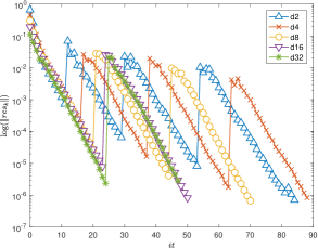
(a) Residual per iteration.

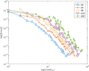
(b) Residual vs. ranks.

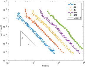
(c) Residual vs. size of support of frames.

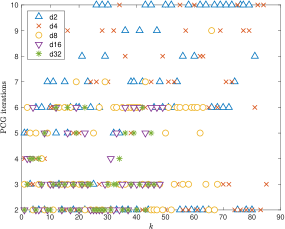
(d) # PCG iterations per HT-AWGM iteration.

Figure 5.1: HT-AWGM for different dimensions $d$.

Results

In Figure 1(a), we display the convergence history with respect to the number of overall iterations. Due to the structure of the linear operator $A$, the condition number $\kappa(\boldsymbol{A}^{\delta})$ is independent of $d$. Moreover, the parameters $\alpha,\omega_{1},\omega_{2}\in(0,1)$ are chosen the same for all dimensions. Thus, the theoretical convergence rate of HT-AWGM is independent of $d$, which is observed in Figure 1(a).

However, the parameters $\omega_{3},\omega_{4},\omega_{5}$ depend on $d$ which result in different tolerances for the re-truncation and re-coarsening step.

In Figure 1(b) we show the behavior of ranks of the numerical solution $\boldsymbol{u}_{k}$. The data points are sorted by rank, where for repeating ranks we took the minimum of the corresponding residual. For all dimensions $d$ we observe an exponential decay w.r.t. ranks, which is according to expectation for the Laplacian. As stated in Remark 4.16 and consistent with the observations in [3], we expect the ranks to scale logarithmically in the dimension.

In Figure 1(c) we plot the sum of the supports of frames and the corresponding residual. Since we are using cubic multi-wavelets, we expect the convergence w.r.t. the support size to be of order 3 and the dimension dependence to be slightly more than linear.

Finally, Figure 1(d) shows the number of PCG iterations in each HT-AWGM iteration. We see that PCG requires between 2 and 10 iterations to achieve a fixed error reduction ($\omega_{2}$) for all dimensions $d$, since $\kappa(\boldsymbol{A}^{\delta})$ does not depend on $d$.

We would like to emphasize that, unlike in classical non-tensor adaptive methods, for high dimensional tensor methods ranks are crucial for performance. The size of the wavelet discretization affects the performance indirectly, since the maximum wavelet level affects the ranks in the preconditioning. However, this is not necessarily a feature solely of the preconditioning. Larger frames imply we are searching for low dimensional manifolds in higher dimensional spaces. In the worst case scenario, this implies the ranks of such manifolds will grow.

A few numerical considerations significantly improve the overall performance. For PCG choosing the adaptive tolerance is a trade off between the number iterations and how expensive each iteration is. We found that choosing the adaptive tolerance $0.1$ yields best results. For experiments varying the adaptive tolerance we refer to [33].

Moreover, note that in each PCG iteration the preconditioned matrix-vector product only has to be computed once, since this can be avoided for computing the energy norm of the search direction. We are only interested in computing the residual and thus we can also avoid computing an intermediate matrix-vector product and apply the preconditioning, summation and truncation to the residual directly. This gives the same result, but involves much lower intermediate ranks, since the truncation tolerances are relative to the residual and not $\|\boldsymbol{A}^{\delta}\boldsymbol{u}_{k}\|$.

Finally, in analogy to [2], if we are interested in controlling the error only in $L_{2}$, we can approximate the $L_{2}$ coefficients. This means applying $\boldsymbol{S}^{-2}(\delta)\boldsymbol{A}$ instead of $\boldsymbol{S}^{-1}(\delta)\boldsymbol{A}\boldsymbol{S}^{-1}(\delta)$ which greatly reduces the computational cost.

Adaptivity

In conclusion we would like to remark on the use of an adaptive discretization for the model problem above. In a classical AWGM method applied to a smooth problem like $-\Delta u=1$, we would expect the algorithm to recover a nearly uniform grid. One might expect the same for the discretization of the frames in a tensor format. However, as we will see, this is not the case.

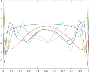
(a) First 6 basis functions.

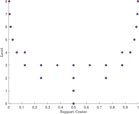
(b) Support centers and levels of wavelets

Figure 5.2: Basis functions in the first dimension for $d=4$.

Figure 2(a) shows the first 6 basis functions in the first dimension of $\boldsymbol{u}_{k}$ for $d=4$ after 15 inner iterations of HT-AWGM. Figure 2(b) shows the support centers of active wavelets.

Note that, since we are using cubic multiwavelets, there are more than one mother scaling functions and mother wavelets. Thus, each point in the plot can possibly represent more than one wavelet. In this particular case the overall number of active wavelets is 66 and the maximum level is 8. The number of wavelets for a uniform grid of up to level 8 is 1536, which is roughly 23 times more than the number of active wavelets at this stage. Recall that the computational complexity is linear in the number of active wavelets.

As we can see, the one dimensional basis functions exhibit boundary layers and oscillations for increasing rank. A similar pattern is observed in all dimensions for all values of $d$. This behavior can be explained as follows.

Note that the computed one dimensional basis functions do not solve the original $d$-dimensional equation. Instead, one can consider the best rank one update. Given a current approximation $u_{k}$, we compute a rank one update $v=v_{1}\otimes\cdots\otimes v_{d}$ such that

$$J(u_{k}+v)=\min_{w=w_{1}\otimes\cdots\otimes w_{d}\in H^{1}_{0}(\Omega)}J(u_{k}+w),$$

where $J:H^{1}_{0}(\Omega)\rightarrow\mathbb{R}$ is the Dirichlet functional

$$J(u)=\int_{\Omega}\nabla^{2}u\;dx-\int_{\Omega}fu\;dx,$$

for some $f\in L_{2}(\Omega)$. Considering the best approximation in the $j$-th dimension and fixing the rest, we can compute the first variation as

$$\frac{d}{d\tau}J(u_{k}+v_{1}\otimes\cdots(v_{j}+\tau g)\cdots\otimes v_{d})\Bigr{|}_{\tau=0} =$$

(5.1) $$=\kappa_{1}\int_{\Omega_{j}}v_{j}^{\prime}g^{\prime}\;dx_{j}+\kappa_{2}\int_{\Omega_{j}}v_{j}g\;dx_{j}-\langle R^{k}_{j},g\rangle =0,\quad\forall g\in H_{0}^{1}(\Omega_{j}),$$

with

$$\kappa_{1} :=\prod_{i\neq j}\|v_{i}\|^{2}_{L_{2}},\quad\kappa_{2}:=\sum_{k\neq j}\|v_{k}^{\prime}\|^{2}_{L_{2}}\prod_{\begin{subarray}{c}i\neq k,\\ i\neq j\end{subarray}}\|v_{i}\|^{2}_{L_{2}},\quad\epsilon^{-1}:=\frac{\kappa_{2}}{\kappa_{1}}=\sum_{k\neq j}\left(\frac{\|v_{k}^{\prime}\|_{L_{2}}}{\|v_{k}\|_{L_{2}}}\right)^{2},$$

$$\langle R^{k}_{j},g\rangle :=\int_{\Omega_{j}}g\int_{\bigtimes_{i\neq j}\Omega_{i}}f\cdot\otimes_{k\neq j}v_{k}\;dx$$

$$\quad-\int_{\Omega_{j}}g\int_{\bigtimes_{i\neq j}\Omega_{i}}\nabla^{d-1,\neq j}u_{k}\cdot\nabla^{d-1,\neq j}\otimes_{k\neq j}v_{k}\;dx$$

(5.2) $$\quad-\int_{\Omega_{j}}g^{\prime}\int_{\bigtimes_{i\neq j}\Omega_{i}}\frac{\partial u_{k}}{\partial x_{j}}\cdot\otimes_{k\neq j}v_{k}\;dx.$$

I.e., the basis functions in Figure 2(a) solve Eq. 5.1. This has two consequences. First, this is no longer a Poisson equation, but rather a reaction-diffusion equation that is singularly perturbed for $\epsilon\rightarrow 0^{+}$. Indeed, we have observed that $\epsilon$ becomes smaller as the rank grows. This explains the boundary layers and the adaptive discretization in Figure 5.2. Second, the right hand side in Eq. 5.1 is the residual from Eq. 5.2. This term has 2 orders of regularity less than the numerical approximation $u_{k}$. I.e., using basis functions of higher regularity improves the regularity of the residual and thus the behavior of the frames of the numerical approximation. Moreover, the residual also introduces the oscillations visible in Figure 2(a).

6 Conclusion

We introduced and analyzed an adaptive wavelet Galerkin
scheme for high dimensional elliptic equations. To deal with the curse of dimensionality, we utilized low rank tensor methods, specifically the Hierarchical Tucker format. The method is adaptive both in the wavelet representation and the tensor ranks.

We have shown that the method converges and that the numerical solution has quasi-optimal ranks and wavelet representation. The computational complexity depends solely on the Besov regularity and low rank approximability of the solution. We provided numerical experiments for the Poisson equation for $d=2,4,8,16$ and $32$ dimensions.

The method is well suited for problems where $d$ is large, provided certain favorable separability assumptions are satisfied: the operator is either low rank or can be accurately approximated by low rank operators; the condition of the operator only mildly depends on the dimension; the right hand side is either low rank or can be accurately approximated by low rank functions. The dominating part of the complexity for HT-AWGM are the ranks. Nonetheless, adaptivity in the wavelet representation pays off computationally even for smooth problems like the Poisson equation.

HT-AWGM involves a re-truncation and a re-coarsening step to ensure optimality w.r.t. ranks and wavelet representation. Although there are evidence to support that both can be avoided, we were not able to devise a rigorous framework to show this. In future work we want to construct a more clever rank extension strategy, avoid both the re-truncation and re-coarsening steps and consider different Galerkin solvers.

References

- [1] Bachmayr, M., and Dahmen, W. Adaptive near-optimal rank tensor approximation for high-dimensional operator equations. Found. Comput. Math. 15, 4 (2015), 839–898.
- [2] Bachmayr, M., and Dahmen, W. Adaptive low-rank methods for problems on Sobolev spaces with error control in . ESAIM Math. Model. Numer. Anal. 50, 4 (2016), 1107–1136.
- [3] Bachmayr, M., and Dahmen, W. Adaptive low-rank methods: problems on Sobolev spaces. SIAM J. Numer. Anal. 54, 2 (2016), 744–796.
- [4] Bachmayr, M., and Schneider, R. Iterative methods based on soft thresholding of hierarchical tensors. Found. Comput. Math. 17, 4 (2017), 1037–1083.
- [5] Bachmayr, M., Schneider, R., and Uschmajew, A. Tensor networks and hierarchical tensors for the solution of high-dimensional partial differential equations. Found. Comput. Math. (2016), 1–50.
- [6] Ballani, J., and Grasedyck, L. A projection method to solve linear systems in tensor format. Numer. Linear Algebra Appl. 20, 1 (2013), 27–43.
- [7] Cohen, A., Dahmen, W., and DeVore, R. Adaptive wavelet methods for elliptic operator equations: convergence rates. Math. Comp. 70, 233 (2001), 27–75.
- [8] Cohen, A., Dahmen, W., and DeVore, R. Adaptive wavelet methods. II. Beyond the elliptic case. Found. Comput. Math. 2, 3 (2002), 203–245.
- [9] Dahmen, W., DeVore, R., Grasedyck, L., and Süli, E. Tensor-sparsity of solutions to high-dimensional elliptic partial differential equations. Found. Comput. Math. 16, 4 (2016), 813–874.
- [10] DeVore, R. A. Nonlinear approximation. In Acta numerica, 1998, vol. 7 of Acta Numer. Cambridge Univ. Press, Cambridge, 1998, pp. 51–150.
- [11] Dolgov, S., and Khoromskij, B. Simultaneous state-time approximation of the chemical master equation using tensor product formats. Numer. Linear Algebra Appl. 22, 2 (2015), 197–219.
- [12] Fischer, B. Polynomial based iteration methods for symmetric linear systems. Wiley-Teubner Series Advances in Numerical Mathematics. John Wiley & Sons, Ltd., Chichester; B. G. Teubner, Stuttgart, 1996.
- [13] Gantumur, T., Harbrecht, H., and Stevenson, R. An optimal adaptive wavelet method without coarsening of the iterands. Math. Comp. 76, 258 (2007), 615–629.
- [14] Hackbusch, W. Iterative Lösung großer schwachbesetzter Gleichungssysteme, vol. 69. B. G. Teubner, Stuttgart, 1991.
- [15] Hackbusch, W. Tensor spaces and numerical tensor calculus, vol. 42 of Springer Series in Computational Mathematics. Springer, Heidelberg, 2012.
- [16] Hackbusch, W., and Kühn, S. A new scheme for the tensor representation. J. Fourier Anal. Appl. 15, 5 (2009), 706–722.
- [17] Holtz, S., Rohwedder, T., and Schneider, R. The alternating linear scheme for tensor optimization in the tensor train format. SIAM J. Sci. Comput. 34, 2 (2012), A683–A713.
- [18] Jarre, F., and Stoer, J. Optimierung. Springer-Verlag, 2004.
- [19] Kestler, S. On the adaptive tensor product wavelet Galerkin Method with applications in finance. PhD thesis, Ulm University, 2013.
- [20] Khoromskij, B. N. Tensor-structured preconditioners and approximate inverse of elliptic operators in . Constr. Approx. 30, 3 (2009), 599–620.
- [21] Khoromskij, B. N., and Oseledets, I. Quantics-TT collocation approximation of parameter-dependent and stochastic elliptic PDEs. Comput. Methods Appl. Math. 10, 4 (2010), 376–394.
- [22] Khoromskij, B. N., and Schwab, C. Tensor-structured Galerkin approximation of parametric and stochastic elliptic PDEs. SIAM J. Sci. Comput. 33, 1 (2011), 364–385.
- [23] Kressner, D., and Tobler, C. Low-rank tensor Krylov subspace methods for parametrized linear systems. SIAM J. Matrix Anal. Appl. 32, 4 (2011), 1288–1316.
- [24] Kreyszig, E. Differential geometry. Dover Publications, Inc., New York, 1991. Reprint of the 1963 edition.
- [25] Nochetto, R. H., Siebert, K. G., and Veeser, A. Theory of adaptive finite element methods: an introduction. In Multiscale, nonlinear and adaptive approximation. Springer, Berlin, 2009, pp. 409–542.
- [26] Novak, E., and Woźniakowski, H. Approximation of infinitely differentiable multivariate functions is intractable. J. Complexity 25, 4 (2009), 398–404.
- [27] Oseledets, I. V. Tensor-train decomposition. SIAM J. Sci. Comput. 33, 5 (2011), 2295–2317.
- [28] Oseledets, I. V., and Dolgov, S. V. Solution of linear systems and matrix inversion in the TT-format. SIAM J. Sci. Comput. 34, 5 (2012), A2718–A2739.
- [29] Rupp, A. High dimensional wavelet methods for structured financial products. PhD thesis, Ulm University, 2013.
- [30] Schneider, R., and Uschmajew, A. Approximation rates for the hierarchical tensor format in periodic Sobolev spaces. J. Complexity 30, 2 (2014), 56–71.
- [31] Stevenson, R. Optimality of a standard adaptive finite element method. Found. Comput. Math. 7, 2 (2007), 245–269.
- [32] Stevenson, R. Adaptive wavelet methods for solving operator equations: an overview. In Multiscale, nonlinear and adaptive approximation. Springer, Berlin, 2009, pp. 543–597.
- [33] Tobler, C. Low-rank tensor methods for linear systems and eigenvalue problems. PhD thesis, ETH Zürich, 2012.
- [34] Urban, K. Wavelet methods for elliptic partial differential equations. Numerical Mathematics and Scientific Computation. Oxford University Press, Oxford, 2009.