An extension of the Gluckstern formulas for multiple scattering: analytic expressions for track parameter resolution using optimum weights

Abstract

Momentum, track angle and impact parameter resolution are key performance parameters that tracking detectors are optimised for. This report presents analytic expressions for the resolution of these parameters for equal and equidistant tracking layers. The expressions for the contribution from position resolution are based on the Gluckstern formulas and are well established. The expressions for the contribution from multiple scattering using optimum weights are discussed in detail.

1 Introduction

The theory of track fitting using global $\chi^{2}$ minimisation is well established [1] [2] and some explicit expressions for geometries with equidistant detector planes are presented in [3] [4] [5]. In this report we derive analytic expressions for the resolution of particle momentum as well as track angle and impact parameter in $r{-}\phi$ and $z$ direction, as defined in Fig. 4. The calculations are performed for a classic solenoid spectrometer with a constant B-field using $N+1$ equal and equidistant detector planes. We present both, the contribution from detector resolution and the contribution from multiple scattering for each of these 5 parameters. In the following, we first present the formalism for $\chi^{2}$ minimisation, then we calculate the covariance matrix of individual measurements, and it’s inverse, assuming detector position resolution and multiple scattering. Then we derive the covariance matrix for the parameters of a straight line track and a parabolic track in an $x{-}y$ coordinate system and finally, we use these results to write down the errors on track parameters in the summary section.

2 General formulas

We assume a particle track of known functional form $f(x)=\sum_{i=0}^{M}a_{i}g_{i}(x)$ with $M+1$ unknown parameters $a_{m}$, and we assume $y_{n}$ to be the measured positions in the $N+1$ detector planes positioned at $x_{n}$. The straight line track in Fig. 2 and the parabolic track in Fig. 3 are the two concrete examples that we will discuss later. The parameters $a_{i}$ are estimated by minimising $\chi^{2}$ defined as

$$\chi^{2}=\sum_{m=0}^{N}\sum_{n=0}^{N}\left[y_{m}-\sum_{i=0}^{M}a_{i}g_{i}(x_{m})\right]\,W_{mn}\,\left[y_{n}-\sum_{i=0}^{M}a_{i}g_{i}(x_{n})\right]$$ (1)

where $W_{mn}$ is the weight matrix that still has to be defined. The above relation can also be written in matrix form

$$\chi^{2}=({\bf y-Ga})^{T}{\bf W(y-Ga)}$$ (2)

with ${\bf a}=(a_{0},a_{1},...,a_{M})$, ${\bf y}=(y_{0},y_{1},...,y_{N})$ and $G_{mn}=g_{n}(x_{m})$. To minimise $\chi^{2}$ we have to solve $\partial\chi^{2}/\partial a_{i}=0$ which gives

$${\bf a}=({\bf G}^{T}{\bf WG})^{-1}{\bf G}^{T}{\bf W\,y}={\bf B\,y}$$ (3)

and represents the estimates for the parameters $a_{i}$. Next we want to know the variance of these estimated parameters for given measurement errors on $y_{n}$. These errors are defined through the covariance matrix ${\bf C_{y}}$ of ${\bf y}$. From error propagation we know that if ${\bf C}_{y}$ is the covariance matrix for ${\bf y}$, the covariance matrix ${\bf C}_{a}$ for ${\bf a}={\bf By}$ is

$${\bf C}_{a}={\bf B}{\bf C}_{y}{\bf B}^{T}=({\bf G}^{T}{\bf WG})^{-1}{\bf G}^{T}{\bf W}\,{\bf C}_{y}\,{\bf W}^{T}{\bf G}({\bf G}^{T}{\bf W}^{T}{\bf G})^{-1}$$ (4)

which is the desired result. The variance of the track position $f(x)$ and track angle $f^{\prime}(x)$ along the track are then given in analogy by

$$(\Delta f(x))^{2}={\bf g}(x)^{T}\,{\bf C}_{a}{\bf g}(x)\qquad\qquad(\Delta f^{\prime}(x))^{2}={\bf g}^{\prime}(x)^{T}\,{\bf C}_{a}{\bf g}^{\prime}(x)$$ (5)

with ${\bf g}(x)=(g_{0}(x),g_{1}(x),...,g_{M}(x))$ and ${\bf g}^{\prime}(x)=(g_{0}^{\prime}(x),g_{1}^{\prime}(x),...,g_{M}^{\prime}(x))$. The weight matrix ${\bf W}$ has to be chosen such that the variances are minimised and the estimators are unbiased. This question is answered by the generalized Gauss-Markov theorem, stating that ${\bf W}={\bf C}_{y}^{-1}$ is the optimum choice. In that case the expression for ${\bf C}_{a}$ reduces to

$${\bf C}_{a}=({\bf G}^{T}{\bf C}_{y}^{-1}{\bf G})^{-1}$$ (6)

3 Covariance matrix $C_{y}$

There are two sources for the measurement errors on $y_{n}$, the position resolution $\sigma_{i}$ of the detector planes, which are uncorrelated, and multiple scattering in the detector planes, which are highly correlated. When assuming thin scatterers, the variance $\sigma_{\alpha_{i}}$ of the multiple scattering angle in a single detector plane is given by [7]

$$\sigma_{\alpha_{i}}=\frac{0.0136\,\mathrm{GeV/c}}{\beta p}\,\sqrt{\frac{d_{i}}{X_{0}}}\left(1+0.038\ln\frac{d_{i}}{X_{0}}\right)=\frac{1}{\beta p[GeV/c]}\,\ f\left(\frac{d_{i}}{X_{0}}\right)$$ (7)

where $d_{i}/X_{0}$ is the thickness of a single detector plane in units of radiation length and

$$f(y)=0.0136\,\mathrm{GeV/c}\sqrt{y}(1+0.038\ln y).$$ (8)

Fig. 1 shows how these errors affect the measurements in the different planes.

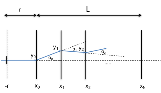
Figure 1: Effect of multiple scattering in the different detector planes.

Assuming that ’for a single event’ we have an offset $u_{n}$, with a mean value of zero and variance $\sigma_{n}^{2}$ due to detector resolution, and a scattering angle $\alpha_{n}$ in the $n^{th}$ detector plane, the measurement values $y_{n}$ are

$$y_{0} = f(x_{0})+u_{0}$$

$$y_{1} = f(x_{1})+u_{1}+\alpha_{0}(x_{1}-x_{0})$$

$$y_{2} = f(x_{2})+u_{2}+\alpha_{0}(x_{2}-x_{0})+\alpha_{1}(x_{2}-x_{1})$$

$$\vdots$$

$$y_{n} = f(x_{n})+u_{n}+\sum_{m=0}^{n-1}\alpha_{m}(x_{n}-x_{m})\qquad n=0,1,...,N$$

The covariance matrix of $y_{n}$ is therefore

$$(C_{y})_{mn}=\sigma_{n}^{2}\delta_{mn}+\sum_{j=0}^{\mathrm{Min}[m,n]-1}\,\sigma_{\alpha_{j}}^{2}\,(x_{m}-x_{j})(x_{n}-x_{j})$$ (9)

In case all detector planes have the same position resolution ($\sigma_{i}^{2}=\sigma^{2}$), the planes are equidistant ($x_{n}=nL/N$, $n=0,1,...,N$) and the detector planes have identical material budget i.e. identical multiple scattering effect ($\sigma_{\alpha_{j}}=\sigma_{\alpha}$), we have

$$(C_{y})_{mn}=\sigma^{2}\delta_{mn}+\frac{\sigma_{\alpha}^{2}}{6}\,\left(\frac{L}{N}\right)^{2}\,n(3m+3mn+1-n^{2})\quad m\geq n\quad\mbox{with}\quad M_{nm}=M_{mn}$$ (10)

This matrix is used to find the covariance matrix ${\bf C}_{a}$ for the combined effect from position resolution and multiple scattering through Eq. 6. In order to be able to derive some elementary formulas we investigate two limiting cases where either the detector resolution dominates or the multiple scattering dominates. In case the detector resolution plays the dominant role we set $\sigma_{\alpha}=0$ and have

$${\bf C}_{y}={\bf R}=\sigma^{2}{\bf 1}\qquad{\bf C}_{y}^{-1}={\bf R}^{-1}=\frac{1}{\sigma^{2}}{\bf 1}$$ (11)

In case multiple scattering dominates we set $\sigma=0$, and the covariance matrix explicitly reads as

$${\bf C}_{y}={\bf M}=\frac{\sigma_{\alpha}^{2}L^{2}}{N^{2}}\left(\begin{array}[]{ccccccccccc}\frac{N^{2}\sigma_{0}^{2}}{\sigma_{\alpha}^{2}L^{2}}&0&0&0&0&0&0&0&.&.&.\\ 0&1&2&3&4&5&6&7&\ldots\\ 0&2&5&8&11&14&17&20&\ldots\\ 0&3&8&14&20&26&32&38&\ldots\\ 0&4&11&20&30&40&50&60&\ldots\\ 0&5&14&26&40&55&70&85&\ldots\\ 0&6&17&32&50&70&91&112&\ldots\\ 0&7&20&38&60&85&112&140&\ldots\\ \vdots&\vdots&\vdots&\vdots&\vdots&\vdots&\vdots&\vdots&\ddots\end{array}\right)$$ (12)

In order to avoid a singular matrix we still keep $\sigma_{0}$ finite and take the limit to zero only for the final result. The inverse of this matrix can be calculated explicitly for every $N$ and is given by

$${\bf C}_{y}^{-1}={\bf M}^{-1}\,=\,\frac{N^{2}}{\sigma_{\alpha}^{2}L^{2}}\left(\begin{array}[]{cccccccccccccc}\frac{L^{2}\sigma_{\alpha}^{2}}{N^{2}{\sigma_{0}}^{2}}&0&0&0&.&.&.&.&.&.&.&.\\ 0&6&-4&1&0&.&.&.&.&.&.&.\\ 0&-4&6&-4&1&0&.&.&.&.&.&.\\ 0&1&-4&6&-4&1&0&.&.&.&.&.\\ .&0&1&-4&6&-4&1&0&.&.&.&.\\ .&.&.&.&.&.&.&.&.&.&.&.\\ .&.&.&.&.&.&.&.&.&.&.&.\\ .&.&.&.&.&.&.&.&.&.&.&.\\ .&.&.&.&.&0&1&-4&6&-4&1&0\\ .&.&.&.&.&.&0&1&-4&6&-4&1\\ .&.&.&.&.&.&.&0&1&-4&5&-2\\ .&.&.&.&.&.&.&.&0&1&-2&1\\ \end{array}\right)$$ (13)

4 Straight line track

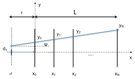
Figure 2: A straight line track through $N+1$ equal and equidistant detector planes.

We assume the geometry shown in Fig. 2 with a straight line track $f(x)=a_{0}+a_{1}x$ through $N+1$ equal and equidistant detector planes. We also assume the track to be almost parallel to the $x$-axis such that $\tan\psi\approx\psi\approx f^{\prime}(x)=a_{1}$ and treat larger track inclinations later in the summary. We have $g_{0}=1$ and $g_{1}=x$, and with $x_{n}=nL/N$ we get

$${\bf G}^{T}=\left(\begin{array}[]{cccccc}1&1&1&1&...&1\\ 0&\frac{L}{N}&\frac{2L}{N}&\frac{3L}{N}&...&L\\ \end{array}\right)$$ (14)

For the contribution from detector resolution we have ${\bf C}_{y}={\bf R}$ and therefore (c.f. Eq. 25 in [3] )

$${\bf C}_{a}=({\bf G}^{T}{\bf R}^{-1}{\bf G})^{-1}=\sigma^{2}({\bf G}^{T}{\bf G})^{-1}=\frac{\sigma^{2}}{(N+1)(N+2)}\left(\begin{array}[]{cc}2(2N+1)&-\frac{6N}{L}\\ -\frac{6N}{L}&\frac{12N}{L^{2}}\end{array}\right)$$ (15)

The variance of the track angle $\Delta\psi=\Delta a_{1}=\sqrt{(C_{a})_{11}}$ is given by

$$\Delta\psi=\frac{\sigma}{L}\sqrt{\frac{12N}{(N+1)(N+2)}}$$ (16)

To find the ’impact parameter’ $d_{1}$ we have $d_{1}=f(-r)$ and with Eq. 5 we find the variance of $d_{1}$ as

$$(\Delta d_{1})^{2}=(\Delta f(-r))^{2} = \frac{4\sigma^{2}}{(N+1)(N+2)}\left[\left(N+\frac{1}{2}\right)+\frac{3Nr}{L}+\frac{3Nr^{2}}{L^{2}}\right]$$ (17)

$$\approx \frac{4\sigma^{2}}{N+3}\left(1+\frac{3r}{L}+\frac{3r^{2}}{L^{2}}\right)\quad\mbox{for}\quad N\gg 1$$ (18)

For very small values of $r/L$ we have $\Delta d_{1}=\sigma/0.91\sigma/0.84\sigma/0.77\sigma$ for $N=1/2/3/4$. For $r/L=1/10$ we have $\Delta d_{1}=1.1\sigma/1.0\sigma/0.95\sigma/0.88\sigma$.

Next we consider the contribution due to multiple scattering, where we first use equal weights for all measurement points to illustrate the difference to optimum weights. We use ${\bf W}={\bf 1}$ and get

$${\bf C}_{a}=({\bf G}^{T}{\bf G})^{-1}({\bf G}^{T}\,{\bf M\,G})({\bf G}^{T}{\bf G})^{-1}=\frac{\sigma_{\alpha}^{2}}{210N(N+1)(N+2)}\times$$ (19)

$$\left(\begin{array}[]{cc}L^{2}(2N^{4}+N^{3}-2N-1)&-L(11N^{4}+16N^{3}-14N^{2}-25N+12)\\[5.69054pt] -L(11N^{4}+16N^{3}-14N^{2}-25N+12)&78N^{4}+312N^{3}+462N^{2}+300N+108\end{array}\right)$$ (20)

The variance of $d_{1}$ is

$$\begin{array}[]{cclc}(\Delta d_{1})^{2}=(\Delta f(-r))^{2}&=&\sigma_{\alpha}^{2}r^{2}&N=1\\[5.69054pt] &=&\sigma_{\alpha}^{2}r^{2}(5/4+L/12r+L^{2}/144r^{2})&N=2\\[5.69054pt] &&\vdots&\\[5.69054pt] &\approx&N\sigma_{\alpha}^{2}r^{2}(39/105+11L/105r+L^{2}/105r^{2})&N\gg 1\end{array}$$ (21)

For $N=1$, i.e for two layers, the $d_{1}$ resolution is $\sigma_{\alpha}r$ and it deteriorates as one introduces more layers, so the equal weights are clearly not ideal for the best measurement precision. Using the optimum weights for the multiple scattering limit i.e. ${\bf W}={\bf M}^{-1}$ from Eq. 13, we find

$${\bf C}_{a}=\lim_{\sigma_{0}\rightarrow 0}({\bf G}^{T}{\bf M}^{-1}{\bf G})^{-1}=\left(\begin{array}[]{cc}0&0\\[5.69054pt] 0&\sigma_{\alpha}^{2}\end{array}\right)$$ (22)

There is no dependence on $N$, so the angular resolution is independent of the number of detector layers

$$\Delta\psi=\sigma_{\alpha}$$ (23)

and equal to the scattering error in a single detector layer. One therefore does not improve the resolution by adding more detector layers, because the additional measurement information is ’cancelled’ by the additional scattering in the detector material. We’ll see later that this holds only for the straight line fit. For the $d_{1}$ resolution we have

$$\Delta d_{1}=r\,\sigma_{\alpha}$$ (24)

which is also independent of the number of detector layers.

5 Parabolic track

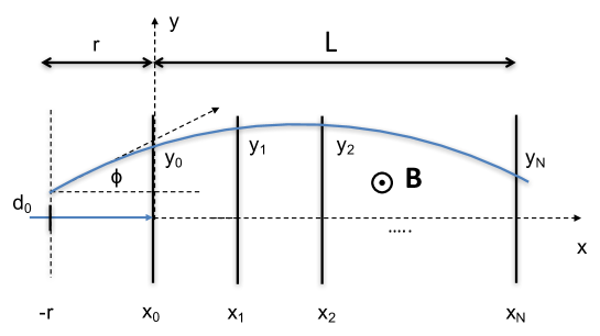
Figure 3: A parabolic track through $N+1$ equal and equidistant detector planes.

We assume the geometry shown in Fig. 3 where a particle of momentum $p$ describes a circle of radius $R$[m]=$p$[GeV/c]/(0.3$B$[T]) in the magnetic field. We approximate this circle by $f(x)=a_{0}+a_{1}x+a_{2}x^{2}/2$ with $a_{2}=1/R$, such that the momentum resolution becomes

$$\frac{\Delta p}{p}=\frac{p}{0.3B}\,\Delta a_{2}$$ (25)

As for the straight line track we assume $a_{1}$ to be small such that $\tan\phi\approx\phi\approx f^{\prime}(x)=a_{1}+a_{2}x$ along the track. We have $g_{0}=1,g_{1}=x,g_{2}=x^{2}/2$ and therefore

$${\bf G}^{T}=\left(\begin{array}[]{cccccc}1&1&1&1&...&1\\ 0&\frac{L}{N}&\frac{2L}{N}&\frac{3L}{N}&...&L\\ 0&\frac{1}{2}\left(\frac{L}{N}\right)^{2}&\frac{1}{2}\left(\frac{2L}{N}\right)^{2}&\frac{1}{2}\left(\frac{3L}{N}\right)^{2}&...&\frac{1}{2}L^{2}\end{array}\right)$$ (26)

and the covariance matrix for the case where the detector resolution $\sigma$ dominates over multiple scattering is (c.f. Eq. 13 in [3])

$${\bf C}_{a}=({\bf G}^{T}{\bf R}^{-1}{\bf G})^{-1}=\frac{\sigma^{2}}{(N+1)(N+2)(N+3)}\left(\begin{array}[]{ccc}9N(N+1)+6&-\frac{18N(2N+1)}{L}&\frac{60N^{2}}{L^{2}}\\ -\frac{18N(2N+1)}{L}&\frac{12N(2N+1)(8N-3)}{L^{2}(N-1)}&-\frac{360N^{3}}{L^{3}(N-1)}\\ \frac{60N^{2}}{L^{2}}&-\frac{360N^{3}}{L^{3}(N-1)}&\frac{720N^{3}}{L^{4}(N-1)}\\ \end{array}\right)$$ (27)

The momentum resolution is therefore

$$\frac{\Delta p}{p}=\frac{p}{0.3B}\,\sqrt{(C_{a})_{22}}=\frac{\sigma\,p}{0.3B\,L^{2}}\sqrt{\frac{720N^{3}}{(N-1)(N+1)(N+2)(N+3)}}$$ (28)

The variance on the track angle $\phi$ reads as

$$(\Delta f^{\prime}(-r))^{2}=\frac{12\sigma^{2}}{L^{2}(N-1)(N+1)(N+2)(N+3)}\left((16N^{3}+2N^{2}-3N)+\frac{60N^{3}\,r}{L}+\frac{60N^{3}\,r^{2}}{L^{2}}\right)$$ (29)

The $d_{0}$ resolution is explicitly written in Eq. 6.4 and for large values of $N$ it is approximated by

$$(\Delta d_{0})^{2}=(\Delta f(-r))^{2} \approx \frac{9\sigma^{2}}{N+5}\left(1+\frac{8r}{L}+\frac{28r^{2}}{L^{2}}+\frac{40r^{3}}{L^{3}}+\frac{20r^{4}}{L^{4}}\right)$$ (30)

For very small values of $r/L$ Eq. 6.4 gives $\Delta d_{0}=\sigma/0.97\sigma/0.94\sigma/0.91\sigma$ for $N=2/3/4/5$. We see that the $d_{1}$ resolution for 2 layers is the same as the $d_{0}$ resolution for 3 layers, and for larger values of $N$ the $d_{0}$ resolution is always worse and approaches a ratio of $\sqrt{9/4}=1.5$ for large values of $N$. This reflects the fact that for the parabola there are 3 degrees of freedom while for the straight line there are only two. For $r/L=1/10$ Eq. 6.4 gives $\Delta d_{0}=1.4\sigma/1.37\sigma/1.34\sigma/1.29\sigma$ for $N=2/3/4/5$, significantly worse than $\Delta d_{1}$ from the straight line track.
For the situation where multiple scattering dominates we first apply equal weights in order to make the link to the results in [3] and to specifically see the difference to optimum weights for the momentum resolution. With ${\bf W}{=}{\bf 1}$ we have

$${\bf C}_{a}=({\bf G}^{T}{\bf G})^{-1}({\bf G}^{T}{\bf M}{\bf G})({\bf G}^{T}{\bf G})^{-1}$$ (31)

and just quote the following elements from this matrix:

$$(C_{a})_{11} = \sigma_{\alpha}^{2}\,\frac{16N^{6}+81N^{5}+234N^{4}+321N^{3}+284N^{2}-228N-108}{70(N-1)(N+1)(N+2)(N+3)N}\approx\sigma_{\alpha}^{2}N\frac{8}{35}$$ (32)

$$(C_{a})_{12} = -\sigma_{\alpha}^{2}\,\frac{N\left(3N^{4}+5N^{3}+15N^{2}+55N+162\right)}{14L(N-1)(N+1)(N+2)(N+3)}\approx-\frac{\sigma_{\alpha}^{2}N}{L}\frac{3}{14}$$ (33)

$$(C_{a})_{22} = \sigma_{\alpha}^{2}\,\frac{10N\left(N^{4}+4N^{3}+5N^{2}+2N+12\right)}{7L^{2}(N-1)(N+1)(N+2)(N+3)}\approx\frac{\sigma_{\alpha}^{2}N}{L^{2}}\frac{10}{7}$$ (34)

The limits of $10/7,3/14,8/35$ for large values of $N$ represent the limits of $C_{N},D_{N},E_{N}$ in Table 2 of [3]. The momentum resolution for a large number of detector planes therefore becomes

$$\frac{\Delta p}{p}=\frac{p}{0.3B}\sqrt{(C_{a})_{22}}\approx\sqrt{\frac{10}{7}}\,\frac{p\sigma_{\alpha}\,\sqrt{N}}{0.3BL}\approx 1.20\,\frac{p\sigma_{\alpha}\,\sqrt{N}}{0.3BL}\qquad N\gg 1$$ (35)

It is quoted in [6] and [3] that this factor 1.20 can be turned into unity in the limit of large $N$ for optimum weights, and a numerical evaluation for finite $N$ is given in [1]. Using the optimum weight matrix ${\bf W}={\bf M}^{-1}$ we can derive an explicit expression for $(C_{a})_{22}$. The covariance matrix is

0N−3/4N−1−N2​(N−1)​L0−N2​(N−1)​LN2(N−1)​L2)subscript𝐂𝑎subscript→subscript𝜎00superscriptsuperscript𝐆𝑇superscript𝐌1𝐆1superscriptsubscript𝜎𝛼2fragments 0𝑁34𝑁1fragments𝑁2𝑁1𝐿0fragments𝑁2𝑁1𝐿superscript𝑁2𝑁1superscript𝐿2{\bf C}_{a}=\lim_{\sigma_{0}\rightarrow 0}({\bf G}^{T}{\bf M}^{-1}{\bf G})^{-1}=\sigma_{\alpha}^{2}\,\left(\begin{tabular}[]{ccc}0&0&0\\ 0&$\frac{N-3/4}{N-1}$&$-\frac{N}{2(N-1)L}$\\ 0&$-\frac{N}{2(N-1)L}$&$\frac{N^{2}}{(N-1)L^{2}}$\end{tabular}\right)

000000 (36)

The contribution of multiple scattering to the momentum resolution is therefore

$$\frac{\Delta{p}}{p} = \frac{p}{0.3B}\sqrt{(C_{a})_{22}}$$ (37)

$$= \frac{N}{\sqrt{(N+1)(N-1)}}\,\frac{p\,\sigma_{\alpha}\sqrt{N+1}}{0.3BL}$$ (38)

$$= (1.15,1.06,1.03,1.02,...)\,\frac{p\,\sigma_{\alpha}\sqrt{N+1}}{0.3BL}\qquad N=2,3,4,5,...$$ (39)

So the factor becomes indeed unity for large $N$ and the convergence is rather fast. Inserting the expression for $\sigma_{\alpha}$ we find

$$\frac{\Delta{p}}{p}=\frac{N}{\sqrt{(N+1)(N-1)}}\,\frac{0.0136\,\mathrm{GeV/c}}{0.3\beta BL}\,\sqrt{\frac{d_{tot}}{X_{0}}}\left(1+0.038\ln\frac{d}{X_{0}}\right)$$ (40)

where $d_{tot}=(N+1)d$ is the total thickness of all detector layers. We see that the contribution to the momentum resolution from multiple scattering is independent on the particle momentum $p$, and is mainly affected by the total material budget. The exception is for small momenta where $\beta=(p/\sqrt{m^{2}c^{2}+p^{2})}$ is different from unity the resolution deteriorates accordingly.
For the resolution of the angle $\phi$ we have

$$\Delta\phi=\Delta f^{\prime}(-r)=\sigma_{\alpha}\,\sqrt{\frac{N-3/4}{N-1}+\frac{N}{N-1}\left(\frac{r}{L}\right)+\frac{N^{2}}{N-1}\left(\frac{r}{L}\right)^{2}}$$ (41)

While for angle of the straight line fit we have $\Delta\psi=\sigma_{\alpha}$ independent on the number of layers, $\Delta\phi$ is larger than $\sigma_{\alpha}$ and shows a dependence on the number of layers. The reason is related to the fact that for the parabola there are 3 instead of 2 degrees of freedom, so the track is less constrained. For 3 layers, i.e. $N{=}2$ and $r/L=1/10$ we have $\Delta\phi{=}1.22\,\sigma_{\alpha}$ i.e. a 22% worse resolution as compared to $\Delta\psi$. The expression actually has a minimum at $N=2+L/2r$ that evaluates to

$$\Delta\phi=\sigma_{\alpha}\sqrt{1+\frac{2r}{L}+\frac{4r^{2}}{L^{2}}}$$ (42)

This means that given an allocated envelope $L$ for the tracker, there is an optimum number of layers inside this envelope that achieves the best possible $\phi$ resolution when considering multiple scattering only. For $r/L=1/10$ the best achievable resolution is $\Delta\phi{=}1.11\,\sigma_{\alpha}$, so around 11 % worse that the $\Delta\psi$ resolution.
The $d_{0}$ resolution is given by the variance of $f(-r)$ and reads as

$$(\Delta d_{0})^{2}=(\Delta f(-r))^{2} = \sigma_{\alpha}^{2}r^{2}\left[\frac{N-3/4}{N-1}+\frac{N}{2(N-1)}\left(\frac{r}{L}\right)+\frac{N^{2}}{4(N-1)}\left(\frac{r}{L}\right)^{2}\right]$$ (43)

This $d_{0}$ resolution also has a minimum at $N=2+L/r$, different from the minimum for the $\phi$ resolution, where it evaluates to

$$(\Delta d_{0})^{2}=\sigma_{\alpha}^{2}r^{2}\left(1+\frac{r}{L}+\frac{r^{2}}{L^{2}}\right)$$ (44)

In typical vertex detector layout, $r\ll L$, and hence $\Delta d_{0}\approx\sigma_{\alpha}r$. By assuming e.g. the first layer at r=2 cm and a radial extent of the vertex tracker of $L=20$ cm we have $L/r=10$ and the optimum $d_{0}$ resolution would be achieved with 13 layers and evaluate to $\Delta d_{0}=1.05\sigma_{\alpha}r$, so only 5% worse than the best possible resolution. For $N=3$ i.e. 4 layers the resolution is $\Delta d_{0}=1.1\sigma_{\alpha}r$, so only 10 % worse than the limit case.
If we assume the distance between layers to be fixed to $D$ and consider adding more and more layers, we have $L=DN$ and the $d_{0}$ resolution approaches $\Delta d_{0}=\sigma_{\alpha}r$ for large numbers of $N$.

6 Summary

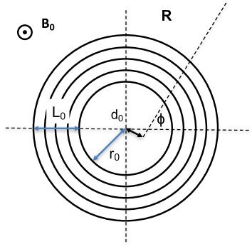
a) b)

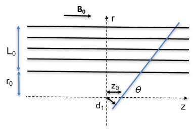
Figure 4: Definition of the track parameters $R,\phi,d_{0},\theta,z_{0}$.

Finally we present the summary of all results from this report, applying the derived expressions from the geometries in Fig. 2 and Fig. 3 to the detector geometry from Fig. 4. The units are $p$ [GeV/c], $p_{T}$ [GeV/c], $L_{0}$ [m], $r_{0}$ [m], $\sigma_{r\phi}$ [m], $\sigma_{z}$ [m] and $B$ [T]. The formulas refer to $N+1$ equidistant detector layers of thickness $d/X_{0}$, where $X_{0}$ is radiation length of the material. The total material budget of this arrangement at perpendicular incident angle is therefore $d_{tot}/X_{0}=(N+1)d/X_{0}$. We have denoted $\sigma_{r\phi}$ as the position resolution in $r{-}\phi$ direction and $\sigma_{z}$ as the resolution in $z-$direction. The factor $\beta$ is related to the momentum by $\beta=(p/\sqrt{m^{2}c^{2}+p^{2})}$. Instead of the angle $\theta$, the pseudorapidity $\eta=-\ln\tan\theta/2$ is used for hadron collisions, so we have $1/\sin\theta=\cosh\eta$ in the following expressions. We define $f(y)=0.0136\,\mathrm{GeV/c}\times\sqrt{y}(1+0.038\ln y)$.

6.1 Momentum resolution

For a track at a given angle $\theta$ the connection between Fig. 3 and Fig. 4a is by $L=L_{0}/\sin\theta,B=B_{0}\sin\theta,p=p_{T}/\sin\theta$ and the amount of traversed material is increased by the factor $1/\sin\theta$, so by inserting this into Eq. 28 and Eq. 40 we have

$$\frac{\Delta p_{T}}{p_{T}}|_{res.} = \frac{\sigma_{r\phi}\,p_{T}}{0.3\,B_{0}L_{0}^{2}}\sqrt{\frac{720N^{3}}{(N-1)(N+1)(N+2)(N+3)}}$$ (45)

$$\approx \frac{12\,\sigma_{r\phi}\,p_{T}}{0.3\,B_{0}L_{0}^{2}}\sqrt{\frac{5}{N+5}}$$ (46)

$$\frac{\Delta p_{T}}{p_{T}}|_{m.s.} = \frac{N}{\sqrt{(N+1)(N-1)}}\,\frac{0.0136\,\mathrm{GeV/c}}{0.3\beta\,B_{0}L_{0}}\,\sqrt{\frac{d_{tot}}{X_{0}\,\sin\theta}}\left(1+0.038\ln\frac{d}{X_{0}\,\sin\theta}\right)$$ (47)

$$\approx \frac{0.0136\,\mathrm{GeV/c}}{0.3\beta\,B_{0}L_{0}}\,\sqrt{\frac{d_{tot}}{X_{0}\,\sin\theta}}$$ (48)

The dependence of momentum resolution on $p_{T}$ and $\theta$ (or $\eta$) has the general form

$$\frac{\Delta p_{T}}{p_{T}}=a\,p_{T}\oplus\frac{b}{\sin^{\frac{1}{2}}\theta}\equiv a\,p_{T}\oplus b\cosh^{\frac{1}{2}}\eta$$ (49)

6.2 Angular resolution in the $r{-}z$ plane

The relation between Fig. 2 and Fig. 4b for Eq. 16 and Eq. 23 is $L=L_{0}/\sin\theta$, $\sigma=\sigma_{z}\sin\theta$, $p=p_{T}/\sin\theta$ and the amount of traversed material is increased by the factor $1/\sin\theta$, so we have

$$\Delta\theta|_{res.} = \frac{\sigma_{z}\,\sin^{2}\theta}{L_{0}}\sqrt{\frac{12N}{(N+1)(N+2)}}$$ (50)

$$\approx \frac{2\,\sigma_{z}\,\sin^{2}\theta}{L_{0}}\sqrt{\frac{3}{N+3}}$$ (51)

$$\Delta\theta|_{m.s.} = \frac{\sin\theta\,}{\beta\,p_{T}}\,f\left(\frac{d}{X_{0}\,\sin\theta}\right)$$ (52)

$$\approx \frac{0.0136\,\mathrm{GeV/c}\,\sin\theta\,}{\beta\,p_{T}}\,\sqrt{\frac{d}{X_{0}\,\sin\theta}}$$ (53)

The dependence of angular resolution in the $r{-}z$ plane on $p_{T}$ and $\theta$ (or $\eta$) has the general form

$$\Delta\theta=a\,\sin^{2}\theta\oplus b\,\frac{\sin^{\frac{1}{2}}\theta}{p_{T}}\equiv\frac{a}{\cosh^{2}\eta}\oplus\frac{b}{p_{T}\cosh^{\frac{1}{2}}\eta}$$ (54)

6.3 Angular resolution in $r{-}\phi$ plane

The relation between Fig. 3 and Fig. 4a for Eq. 29 and Eq. 41 is $r=r_{0}/\sin\theta$, $L=L_{0}/\sin\theta$, $p=p_{T}/\sin\theta$ and we have to multiply the result by $1/\sin\theta$ to project the angle onto the $r{-}\phi$ plane, which gives

$$\Delta\phi|_{res.} = \frac{\sqrt{12}\sigma_{r\phi}}{L_{0}\sqrt{(N-1)(N+1)(N+2)(N+3)}}\sqrt{(16N^{3}+2N^{2}-3N)+\frac{60N^{3}\,r_{0}}{L_{0}}+\frac{60N^{3}\,r_{0}^{2}}{L_{0}^{2}}}$$ (55)

$$\approx \frac{\sigma_{r\phi}}{L_{0}}\frac{8\sqrt{3}}{\sqrt{N+5}}\sqrt{1+\frac{15}{4}\frac{r_{0}}{L_{0}}+\frac{15}{4}\frac{r_{0}^{2}}{L_{0}^{2}}}$$ (56)

$$\Delta\phi|_{m.s.} = \frac{1}{\beta p_{T}}\,f\left(\frac{d}{X_{0}\sin\theta}\right)\sqrt{\frac{N-3/4}{N-1}+\frac{N}{N-1}\left(\frac{r_{0}}{L_{0}}\right)+\frac{N^{2}}{N-1}\left(\frac{r_{0}}{L_{0}}\right)^{2}}$$ (57)

$$\approx \frac{0.0136\,\mathrm{GeV/c}}{\beta p_{T}}\,\sqrt{\frac{d}{X_{0}\sin\theta}}\sqrt{1+\left(\frac{r_{0}}{L_{0}}\right)+\left(\frac{r_{0}}{L_{0}}\right)^{2}}$$ (58)

The dependence of angular resolution in the $r{-}\phi$ plane on $p_{T}$ and $\theta$ (or $\eta$) has the general form

$$\Delta\phi=a\oplus\frac{b}{p_{T}\sin^{\frac{1}{2}}\theta}=a\oplus\frac{b\cosh^{\frac{1}{2}}\eta}{p_{T}}$$ (59)

6.4 Transverse impact parameter resolution

The relation between Fig. 3 and Fig. 4a in Eq. 30 and Eq. 43 is $L=L_{0}/\sin\theta$, $r=r_{0}/\sin\theta$, $p=p_{T}/\sin\theta$ and we get

$$\Delta d_{0}|_{res.} = \frac{3\sigma_{r\phi}}{\sqrt{(N-1)(N+1)(N+2)(N+3)}}\times$$

$$\sqrt{\left(N^{3}-\frac{N}{3}-\frac{2}{3}\right)+\frac{4(2N^{3}-N^{2}-N)r_{0}}{L_{0}}+\frac{4(7N^{3}-N^{2}-N)r_{0}^{2}}{L_{0}^{2}}+\frac{40N^{3}r_{0}^{3}}{L_{0}^{3}}+\frac{20N^{3}r_{0}^{4}}{L_{0}^{4}}}$$

$$\approx \frac{3\sigma_{r\phi}}{\sqrt{N+5}}\sqrt{1+\frac{8r_{0}}{L_{0}}+\frac{28r_{0}^{2}}{L_{0}^{2}}+\frac{40r_{0}^{3}}{L_{0}^{3}}+\frac{20r_{0}^{4}}{L_{0}^{4}}}$$ (61)

$$\Delta d_{0}|_{m.s.} = \frac{r_{0}}{\beta p_{T}}\,f\left(\frac{d}{X_{0}\sin\theta}\right)\sqrt{\frac{N-3/4}{N-1}+\frac{N}{2(N-1)}\left(\frac{r_{0}}{L_{0}}\right)+\frac{N^{2}}{4(N-1)}\left(\frac{r_{0}}{L_{0}}\right)^{2}}\,$$ (62)

$$\approx \frac{0.0136\,\mathrm{GeV/c}}{\beta p_{T}}r_{0}\,\sqrt{\frac{d}{X_{0}\sin\theta}}\sqrt{1+\frac{1}{2}\left(\frac{r_{0}}{L_{0}}\right)+\frac{N}{4}\left(\frac{r_{0}}{L_{0}}\right)^{2}}$$ (63)

The dependence of transverse impact parameter resolution on $p_{T}$ and $\theta$ (or $\eta$) has the general form

$$\Delta d_{0}=a\oplus\frac{b}{p_{T}\sin^{\frac{1}{2}}\theta}=a\oplus\frac{b\cosh^{\frac{1}{2}}\eta}{p_{T}}$$ (64)

6.5 Longitudinal impact parameter resolution

The relation between Fig. 2 and Fig. 4b in Eq. 17 and Eq. 24 is $\Delta z_{0}=\Delta d_{1}/\sin\theta$, $L=L_{0}/\sin\theta$, $r=r_{0}/\sin\theta$, $p=p_{T}/\sin\theta$, $\sigma=\sigma_{z}\sin\theta$ and we get

$$\Delta z_{0}|_{res.} = \frac{2\sigma_{z}}{\sqrt{(N+1)(N+2)}}\sqrt{\left(N+\frac{1}{2}\right)+\frac{3Nr_{0}}{L_{0}}+\frac{3Nr_{0}^{2}}{L_{0}^{2}}}$$

$$\approx \frac{2\sigma_{z}}{\sqrt{N+3}}\sqrt{1+\frac{3r_{0}}{L_{0}}+\frac{3r_{0}^{2}}{L_{0}^{2}}}$$

$$\Delta z_{0}|_{m.s.} = \frac{r_{0}}{\sin\theta}\frac{1}{\beta p_{T}}\,f\left(\frac{d}{X_{0}\sin\theta}\right)$$ (66)

$$\approx \frac{0.0136\,\mathrm{GeV/c}}{\beta p_{T}}\frac{r_{0}}{\sin\theta}\,\sqrt{\frac{d}{X_{0}\sin\theta}}$$ (67)

The dependence of longitudinal impact parameter resolution on $p_{T}$ and $\theta$ (or $\eta$) has the general form

$$\Delta z_{0}=a\oplus\frac{b}{p_{T}\sin^{\frac{3}{2}}\theta}=a\oplus\frac{b\,\cosh^{\frac{3}{2}}\eta}{p_{T}}$$ (68)

7 Bibliography

References

- [1] R. Frühwirth, A. Strandlie, Pattern Recognition and Reconstruction, in Landolt-Börnstein, Elementary Particles, Detectors for Particles and Radiation, ISBN: 978-3-642-03605-7 (Print) 978-3-642-03606-4 (Online)
- [2] R. Mankel, Pattern recognition and event reconstruction in particle physics experiments, Rep. Prog. Phys. 67 (2004) 553-622
- [3] R. L. Gluckstern, Uncertainties in track momentum and direction due to multiple scattering and measurement errors, NIMA 24 (1963) 381-389
- [4] M. Regler, R. Frühwirth, Generalization of the Gluckstern formulas I: Higher orders, alternatives and exact results, NIMA 589 (2008) 109-117
- [5] M. Valentan, M. Regler, R. Frühwirth, Generalization of the Gluckstern formulas II: Multiple scattering and non-zero dip angles, NIMA 606 (2009) 728-742
- [6] W. T. Scott, Correlated Probabilities in Multiple Scattering, Phys. Rev. 76 (1949) 212
- [7] C. Patrignani et al. (Particle Data Group), Chin. Phys. C, 40, 100001 (2016) and 2017 update, Passage of particles through matter.