Abstract

We discuss a new covariant scalar-tensor system aimed to realise Hořava proposal for a power-counting renormalizable theory of gravity, with the special feature of not propagating scalar degrees of freedom in an appropriate gauge. The theory is characterized by a new symmetry acting on the metric, that can protect the particular form of its interactions. The set-up spontaneously breaks Lorentz symmetry by means of a time-like scalar field profile. By selecting a unitary gauge for the scalar, we show that this theory describes the dynamics of a spin two degree of freedom, whose equations of motion contain two time derivatives and up to six spatial derivatives. We analytically determine asymptotically flat, spherically symmetric configurations, showing that there exists a branch of solutions physically equivalent to spherically symmetric configurations in General Relativity, also in the presence of matter fields.

1 Introduction

Understanding the ultraviolet behaviour of Einstein gravity and its possible unitary completion at the Planck scale is one of the deepest open problems in high energy physics. Stelle [1] pointed out that adding specific covariant combinations of the Riemann tensor to the Einstein-Hilbert action makes gravity renormalizable, at the price of introducing an Ostrogradsky ghost mode associated with higher order time derivatives in the field equations. Hořava proposed to eliminate the ghost by renouncing to Lorentz invariance, assigning a special role to the time coordinate, and considering combinations of operators with up to six spatial derivatives of the metric, so to obtain a power counting renormalizable theory of gravity. Starting from the explicit original constructions [2, 3], called Hořava-Lifshitz gravity, a large number of studies have explored this proposal in detail. Both the projectable and non-projectable versions of the theory suffer from strong coupling problems and instabilities linked with the dynamics of a scalar mode associated with the breaking of Lorentz invariance [5, 6, 4]. The healthy extension of the original theory [7] is free from such instabilities and belongs to a class of scenarios called khronometric theories [8, 9]. Its spectrum – besides the healthy scalar – includes instantaneous interactions which make subtle the study of its physical consequences and the proof of renormalizability beyond power counting [10]. The scalar mode can be removed completely [11] by enriching the theory with auxiliary fields with an associated $U(1)$ symmetry, so to make such scalar a pure gauge mode. For the case of projectable Hořava-Lifshitz gravity, issues raised again this possibility (see e.g. [12, 13]), can be solved renouncing to the projectable condition: see e.g. [14]. There are many excellent reviews on all these topics, see e.g. [16, 15, 17].

In this work we build a covariant action for a new scalar-tensor theory aimed to provide a realisation of Hořava proposal, with the specific property that it does not propagate scalar excitations around configurations where the scalar profile satisfies a unitary gauge condition. The theory propagates a single massless spin two tensor mode, that at low energies has the same dynamics as in GR, while at higher energies is characterised by modified dispersion relations as in Hořava scenario. The absence of scalar excitations is a welcome feature both from a theoretical and a phenomenological viewpoint, since it automatically avoids strong coupling and instability issues in the scalar sector, as well as constraints associated with possible gravitational and cosmological effects of so-far-unobserved light scalar modes.

A covariant version of Hořava-Lifshitz gravity is usually constructed by applying a Stückelberg trick to the non-covariant version of Hořava theory: this approach makes manifest the dynamics of the scalar excitation associated with the breaking of general covariance. We take a different route, building our system directly in a covariant way by applying techniques that are currently being developed to investigate scalar-tensor theories, in particular the properties of disformal transformations [18]. It is well known that a combination of disformal and conformal transformations (see e.g. [20, 19, 21, 22]) can be used to build classes of scalar-tensor theories characterized by higher order equations of motion, but that nevertheless do not propagate Ostrogradsky ghosts thanks to the presence of constraint conditions. Such examples belong to the class of covariant, degenerate higher order scalar-tensor theories [23, 24, 25, 26, 27] which propagate at most three degrees of freedom despite having equations of motion containing more than two time derivatives.

Here we show that a suitable limit of a disformal transformation acting on a purely gravitational set-up leads to a scalar-tensor system which spontaneously breaks Lorentz symmetry, selecting a time-like scalar profile. The scalar-tensor interactions are invariant under a new symmetry acting on the metric. By selecting a special foliation for the space-time – which corresponds to a unitary gauge for the scalar field, and is motivated by our pattern of spontaneous Lorentz symmetry breaking – we determine a set-up that does not propagate scalar degrees of freedom, but only a massless spin two tensor mode, whose equations of motion contain two time and at most six spatial derivatives. Our system can be seen as a generalization of the cuscuton [28] and cuscuta-Galileon [29, 30] theories. The available parameters can be chosen such to reproduce GR results for the low energy, linearised propagation of tensor modes, while the tensor dispersion relations are modified at high energies, potentially realising Hořava proposal of a power counting renormalizable theory of gravity. Our system allows also to analytically study spherically symmetric configurations: we show that there are two branches of asymptotically flat solutions, one of which coincides with GR configurations, the other predicts subleading modifications to GR results at large distances from a source.

Our presentation proceeds as follows. In Section 2 we explain how we construct a theory with the aforementioned properties. In Section 3 we prove that the theory only propagates tensor modes in a unitary gauge for the scalar, whose equations of motion are characterised by higher spatial derivatives. In Section 4 we discuss phenomenological consequences of modified dispersion relations for linearised tensor perturbations, and the properties of spherically symmetric solutions. We conclude in Section 5.

2 The construction of the theory

We develop a method for building covariant scalar-tensor couplings that spontaneously break Lorentz invariance, and whose properties prevent the propagation of scalar degrees of freedom in a unitary gauge. The resulting theory propagates a single dynamical spin two mode, whose dispersion relations are modified at high energies with respect to Einstein gravity.

We start with an action $S_{gr}$ which is a combination of covariant Lagrangian densities involving only the metric tensor and its derivatives

$${S}_{gr} = \frac{M_{Pl}^{2}}{2}\,\int\,d^{4}x\,\epsilon\,\sqrt{-g}\,\left[{\cal L}_{R^{(1)}}+{\cal L}_{R^{(2)}}+{\cal L}_{R^{(3)}}\right]\,,$$ (1)

with $\epsilon$ a constant dimensionless parameter (that eventually will be sent to zero) and

$${\cal L}_{R^{(1)}} = {g_{1}}\,R\,,$$ (2)

$$M_{Pl}^{2}\,{\cal L}_{R^{(2)}} = {g_{2}}\,R^{2}+\,g_{3}\,R_{\mu\nu}R^{\mu\nu}\,,$$ (3)

$$M_{Pl}^{4}\,{\cal L}_{R^{(3)}} = {g_{4}}\,R^{3}+g_{5}\,R\,R_{\mu\nu}R^{\mu\nu}+g_{6}\,R_{\mu\rho}R^{\rho\sigma}R_{\sigma}^{\,\,\mu}+g_{7}\,R\,\Box\,R+g_{8}\,\left(\nabla_{\mu}R_{\nu\sigma}\right)^{2}\,,$$ (4)

and $g_{i}$ are constants . Up to total derivatives, these are the most general parity preserving covariant combinations of Ricci curvature with up to six derivatives acting on the metric . We apply a specific disformal transformation to the action $S_{gr}$ of eq (1), defined in terms of a scalar field $\phi$ and the parameter $\epsilon$ as

$$g_{\mu\nu}\to g_{\mu\nu}-\frac{1}{\epsilon^{2}\,\Lambda^{4}}\,\partial_{\mu}\phi\partial_{\nu}\phi\,,$$ (5)

with inverse

$$g^{\mu\nu}\,\to\,g^{\mu\nu}+\frac{1}{\epsilon^{2}\,\Lambda^{4}+X}\,\partial^{\mu}\phi\,\partial^{\nu}\phi\,,$$ (6)

where

$$X\,=\,-\partial^{\mu}\phi\partial_{\mu}\phi\,$$ (7)

and $\Lambda$ is a mass scale that from now on we set to one: $\Lambda=1$. We are interested in the ‘singular’ limit of small (eventually vanishing) parameter $\epsilon$: such limit leads to a theory with especially interesting properties, at least in a unitary gauge for the scalar.

The small $\epsilon$ limit of the disformal transformation, which we indicate with the symbol $\Rightarrow$, when applied to the building blocks of the previous action gives

$$g^{\mu\nu} \Rightarrow g_{dis}^{\mu\nu}\,=\,g^{\mu\nu}+\frac{1}{X}\,\partial^{\mu}\phi\,\partial^{\nu}\phi\,,$$ (8)

$$\sqrt{-g} \Rightarrow \sqrt{-g_{dis}}\,=\,\frac{1}{\epsilon}\sqrt{X}\,\sqrt{-g}\,,$$ (9)

$$R \Rightarrow R_{dis}\,=\,\frac{2\left\langle\Phi^{2}\right\rangle}{X^{2}}+\frac{\left[\Phi^{2}\right]}{{X}}+{R}{}-\frac{2\langle\Phi\rangle([\Phi])}{X^{2}}-\frac{{[\Phi]}^{2}}{{X}}+\frac{2R^{\mu\nu}\partial_{\mu}\phi\partial_{\nu}\phi}{{X}}\,,$$ (10)

$$R_{\mu\nu} \Rightarrow R^{dis}_{\mu\nu}\,=\,R_{\mu\nu}+\frac{\partial^{\alpha}\phi\Phi_{\alpha\mu}\Phi_{\beta\nu}\partial^{\beta}\phi}{X^{2}}+\frac{R_{\mu\alpha\nu\beta}\partial^{\alpha}\phi\partial^{\beta}\phi}{X}+\frac{\Phi_{\alpha\mu}\Phi_{\nu}^{\alpha}}{X}-\frac{\Phi_{\mu\nu}\langle\Phi\rangle}{X^{2}}-\frac{\Phi_{\mu\nu}{[\Phi]}}{X}\,,$$

where $\Phi$ is a matrix with components $\nabla^{\mu}\nabla_{\nu}\phi$, and

$$[\Phi^{n}] =\text{tr}(\Phi^{n})\,,$$ (12)

$$\langle\Phi^{n}\rangle =\partial\phi\cdot\Phi^{n}\cdot\partial\phi\,.$$ (13)

In expressions (8)-(LABEL:rmunu-df) we only write the contributions that are leading in a small $\epsilon$ expansion, neglecting the higher order terms. The structure of the disformed action, which we call $\tilde{S}_{\phi}$, can be obtained by combining the results above: it is sufficient to substitute the disformed expressions for the inverse metric, the Ricci tensor, etc. contained in eqs (8)-(LABEL:rmunu-df) into the initial Lagrangians (2)-(4). The resulting disformed system, in the zero $\epsilon$ limit, is described by the scalar-tensor action $\tilde{S}_{\phi}$ as

$${\tilde{S}}_{\phi} = \frac{M_{Pl}^{2}}{2}\,\int\,d^{4}x\,\sqrt{-g}\,\left[\tilde{\cal L}_{R^{(1)}}+\,\tilde{\cal L}_{R^{(2)}}+\,\tilde{\cal L}_{R^{(3)}}\right]$$ (14)

$$\equiv \frac{M_{Pl}^{2}}{2}\,\int\,d^{4}x\,L_{\phi}\,.$$ (15)

Notice that the factor of $\epsilon$ in eq (1) gets compensated by inverse powers of $\epsilon$ in the disformed quantities – and terms with positive powers of $\epsilon$ vanish in the small $\epsilon$ limit. The expression for $\tilde{\cal L}_{R^{(1)}}$ is relatively simple, but non-analytic since it contains a $\sqrt{X}$, and reads

$$\tilde{\cal L}_{R^{(1)}}\,=\,g_{1}\,{\sqrt{\vphantom{X^{2}}X}}\left[R+\frac{{[\Phi]}^{2}}{X}-\frac{{[\Phi^{2}]}}{X}\right]\,.$$ (16)

The covariant expressions for the $\tilde{\cal L}_{R^{(2,\,3)}}$ are more complex, but – as explained above – can be straightforwardly obtained by combining the disformed building blocks of eqs (8)-(LABEL:rmunu-df). As an example, in Appendix A we express the disformed Lagrangian $\tilde{\cal L}_{R^{(2)}}$. Its covariant expression, and the one of $\tilde{\cal L}_{R^{(3)}}$, is again non-analytic. Their structure makes them covariantized relatives of cuscuton and cuscuta-Galileon theories [28, 30, 29], which are known as not propagating scalar modes around a special foliation [32, 33].

The resulting theory has the following properties, which we will use in what follows:

• Symmetries: Since the original theory, eq (1), is built only in terms of the metric, any transformation that leaves invariant the combination built in (5), corresponding to the disformed metric, will be a symmetry of the final theory $\tilde{S}_{\phi}$. One of such transformations is

  $$\phi \to \phi+\epsilon^{2}\chi\,,$$ (17)

  $$g_{\mu\nu} \to g_{\mu\nu}+\partial_{\mu}\chi\partial_{\nu}\phi+\partial_{\mu}\phi\partial_{\nu}\chi+\epsilon^{2}\partial_{\mu}\chi\partial_{\nu}\chi\,,$$ (18)

  for an arbitrary scalar $\chi$. In the limit $\epsilon\to 0$ we are considering, it reduces to a transformation that involves the metric only

  $$g_{\mu\nu} \to g_{\mu\nu}+\partial_{\mu}\chi\partial_{\nu}\phi+\partial_{\mu}\phi\partial_{\nu}\chi\,.$$ (19)

  Consequently, the transformation (19) is a symmetry for the disformed action $\tilde{S}_{\phi}$: it is valid for any arbitrary scalar function $\chi$. A posteriori, this symmetry can motivate, and possibly protect, the specific structure of our scalar-tensor interactions that form $\tilde{S}_{\phi}$ in eq (14). We shall discuss in Section 3 its consequences for characterising the number of propagating degrees of freedom .

• Preferred foliation of space-time: Given the non-analytic structure of our theory – due to the presence of square roots and inverse powers of $X$, see eqs (8) – the scalar necessarily acquires a time-like profile : $\nabla_{\mu}\phi\,\nabla^{\mu}\phi<0$. This implies that Lorentz invariance is spontaneously broken around any configuration solving the equations of motion. Given that Lorentz symmetry is broken, it is natural to select a preferred foliation for space-time corresponding to a unitary gauge for the scalar field, where constant time hypersurfaces coincide with constant scalar hypersurfaces. Such preferred foliation is special since around it a reduced number of degrees of freedom propagate, as we shall prove later.

• Constraint equation: Besides symmetry (19), it is straightforward to explicitly check that the ‘energy-momentum tensor’ for this set-up, which we define as ($L_{\phi}$ given in (14))

  $$T_{\mu\nu}\,=\,-\frac{2}{\sqrt{-g}}\,\frac{\delta{L}_{\phi}}{\delta g^{\mu\nu}}\,,$$ (20)

  automatically satisfies the relation

  $$T_{\mu\nu}\,\partial^{\nu}\phi\,=\,0$$ (21)

  as a constraint, independently of the equations of motion: in a sense it is an analogue of the Bianchi identity satisfied by the Einstein tensor in General Relativity. We will make use of the covariant condition (21) when studying the time evolution of the ADM constraints in Section 3.2.

The action ${\tilde{S}}_{\phi}$ has a peculiar feature: it does not propagate tensor nor scalar degrees of freedom, at least in a unitary gauge where the scalar field $\phi$ depends only on time. This statement appears at first sight surprising: the resulting action contains kinetically mixed scalar and tensor degrees of freedom, and moreover manifestly leads to equations of motion of order higher than two – hence potentially propagating Ostrogradsky ghosts.

We shall develop a proof of this statement in Section 3: here we provide some initial heuristic arguments in its favour, and discuss some of its consequences in view of a possible realisation of Hořava idea of a power-counting renormalizable theory of gravity. The fact that a theory described by action ${\tilde{S}}_{\phi}$ does not propagate scalar modes, despite manifestly containing a scalar field $\phi$, can be understood from the fact that the theory is built from a disformal transformation of a theory $S_{gr}$ constructed only in terms of the metric tensor: the final action ${\tilde{S}}_{\phi}$ has the gauge symmetry (19) that we can use to ‘gauge away’ a propagating degree of freedom (analogously to the Maxwell action for electromagnetism, where the $U(1)$ symmetry prevents the propagation of the photon longitudinal mode, making it a pure gauge). The property that ${\tilde{S}}_{\phi}$ does not propagate tensors either, selecting a unitary gauge for the scalar profile $\phi\,=\,\phi(t)$ is due to the fact that tensor fluctuations around any given background do not contain any time derivatives, but only spatial derivatives. This feature was noticed in [22, 39, 27] for the particular case of $\tilde{\cal L}_{R^{(1)}}$, which is a special case of quartic Horndeski. But the same property holds also for $\tilde{\cal L}_{R^{(2,\,3)}}$: in unitary gauge, the action for the tensor mode contains spatial derivatives only, that are not sufficient for making it a propagating mode.

Since $\tilde{S}_{\phi}$ does not propagate any degree of freedom in unitary gauge, it might appear of little interest. However, we can add $\tilde{S}_{\phi}$ to the Einstein-Hilbert action, and write a complete system

$$S_{T} = S_{EH}+\tilde{S}_{\phi}$$ (22)

$$= \frac{M_{Pl}^{2}}{2}\,\int\sqrt{-g}\,R+\tilde{S}_{\phi}\,.$$ (23)

The Einstein-Hilbert part provides a standard kinetic term for the tensor mode – but the additional contribution of $\tilde{S}_{\phi}$ includes higher spatial derivatives to the action, and modify the tensor dispersion relations. The covariant scalar-tensor theory $S_{T}$, once a unitary gauge $\phi=\phi(t)$ is selected, contains spatial derivatives up to sixth order acting on the metric, and up to two time derivatives. Hence in a high energy regime – where the effects of the higher derivatives in ${\tilde{\cal L}}_{R^{(3)}}$ become more and more relevant – the theory becomes power counting renormalizable, providing a specific realization of Hořava proposal [3] . Interestingly, the presence of the Einstein-Hilbert term breaks the symmetry (19), but still the scalar-tensor system described by $S_{T}$ does not propagate scalar excitations in the unitary gauge $\phi(t)$.

Since some of the contributions to our action are obtained from a singular limit of a disformal transformation, our scenario might be related with the proposal of mimetic gravity [37]. A complete clarification of possible connections with this theory go beyond the scope of this paper: on the other hand, we point out that our final action for gravity is the sum of the disformed action $\tilde{S}_{\phi}$ and the standard Einstein-Hilbert term, see eq (22), which is not obtained from a disformal transformation. Instead, an alternative realisation of a covariant renormalizable theory of gravity which is more directly connected with mimetic gravity can be found in [38].

3 The propagating degrees of freedom

We now investigate the dynamics of propagating degrees of freedom for the action (22). We first study the theory in flat space, and show explicitly that a residual symmetry remains that, in combination with diffeomorphisms, prevents the propagation of scalar modes. We then make use of a covariant ADM formulation of the system to show that, when a unitary gauge is selected for the scalar field, the theory does not propagate scalars around any background, and the corresponding equations of motion act with higher spatial derivatives only on the tensor sector.

3.1 A residual symmetry in flat space-time removes the scalar excitation

As mentioned in Section 2, the Einstein-Hilbert contribution to action (22) breaks the symmetry (19) obeyed by $\tilde{S}_{\phi}$: nevertheless a residual symmetry remains around flat space, preventing the propagation of scalar modes. We show this fact explicitly in this Section, discussing an interesting interplay between the symmetry (19) and diffeomorphism invariance of the system.

Computing the field equations for the metric and scalar field associated with action (22), one finds they are satisfied for a flat space and for a time-like field profile

$$\bar{\phi}\,=\,c_{\mu}x^{\mu}\,,$$ (24)

for constant $c^{\mu}$ satisfying $c_{\mu}\,c_{\nu}\,\eta^{\mu\nu}\,<\,0$. We can study the dynamics of fluctuations around a background metric and scalar

$$g_{\mu\nu} = \eta_{\mu\nu}+h_{\mu\nu}\,,$$ (25)

$$\phi = \bar{\phi}+\delta\phi\,.$$ (26)

We now exploit symmetry arguments to demonstrate that, around flat space, $\delta\phi$ is not dynamical since it is pure gauge. The quadratic action for fluctuations associated with the total action $S_{T}$ of eq (22) is made of two contributions. The Einstein-Hilbert part $S_{EH}$ is invariant under infinitesimal diffeomorphisms:

$$h_{\mu\nu}\,\to\,h_{\mu\nu}+\partial_{\mu}\xi_{\nu}+\partial_{\nu}\xi_{\mu}\,,$$ (27)

for arbitrary functions $\xi_{\mu}$. For what respect $\tilde{S}_{\phi}$, we notice that the scalar field profile (24) spontaneously breaks the diffeomorphism symmetry: under infinitesimal diffeos, the scalar fluctuation transforms non-linearly as

$$\delta\phi\to\delta\phi+\partial_{\mu}\bar{\phi}\,\xi^{\mu}\,.$$ (28)

On the other hand, we know that $\tilde{S}_{\phi}$ is invariant under the transformation (19):

$$h_{\mu\nu}\to h_{\mu\nu}+\partial_{\mu}\bar{\phi}\,\partial_{\nu}\chi+\partial_{\mu}\chi\,\partial_{\nu}\bar{\phi}\,,$$ (29)

for an arbitrary scalar function $\chi$. This symmetry can be used to ‘compensate’ the spontaneous breaking of diffeomorphism by the scalar profile of eq (28). Indeed, exploiting the transformation (28), we can select a special unitary gauge choice (selecting appropriately a profile for $\xi^{\mu}$) to set to zero the scalar fluctuations, transferring the scalar dof into the metric sector:

$$\bar{\xi}^{\mu}\,=\,\frac{\partial^{\mu}\bar{\phi}}{\bar{X}}\,\delta\phi\,,$$ (30)

with

$$\bar{X}\,=\,-\partial_{\rho}\bar{\phi}\partial^{\rho}\bar{\phi}\,.$$ (31)

Making this choice of diffeomorphism parameter, we learn that under diffeomorphisms the field fluctuations transform as

$$\delta\phi \to 0\,,$$ (32)

$$h_{\mu\nu} \to h_{\mu\nu}+\partial_{\mu}\bar{\xi}_{\nu}+\partial_{\nu}\bar{\xi}_{\mu}\,=\,h_{\mu\nu}+\frac{1}{\bar{X}}\partial_{\mu}\bar{\phi}\,\partial_{\nu}\delta\phi+\frac{1}{\bar{X}}\partial_{\nu}\bar{\phi}\,\partial_{\mu}\delta\phi\,,$$ (33)

where we used the field profile of eq (24). Such specific choice of diffeomorphism parameter $\xi^{\mu}$ does not affect the counting of degrees of freedom in the Einstein-Hilbert action (which is invariant under diffeos) but it can affect $\tilde{S}_{\phi}$, where diffeos are spontaneously broken. But we can now use symmetry (29) to compensate the contributions to the metric in eq (33), by applying transformation (29) to eq (33) and choosing

$$\chi\,=\,-\frac{\delta\phi}{\bar{X}}\,,$$ (34)

so to make $h_{\mu\nu}$ invariant under a combination of diffeo and scalar transformations, as desired.

Hence, using the symmetries available around flat space we learn that scalar fluctuations are pure gauge and do not propagate: diffeomorphisms and the scalar symmetry (19) combine together to eliminate scalar fluctuations, even in the presence of a non-vanishing background scalar profile. In the next Section, we show with a more general method that the same remains true around curved space-time, at least when selecting a unitary gauge for the scalar field.

3.2 Counting the degrees of freedom in curved space-time in unitary gauge

We now consider the curved space-time case, where the equations of motion for the metric in our theory (22) read

$$G_{\mu\nu}\,=\,\frac{1}{M_{Pl}^{2}}\,T_{\mu\nu}\,,$$ (35)

with $G_{\mu\nu}$ the Einstein tensor, and $T_{\mu\nu}$ the energy momentum tensor associated with $\tilde{S}_{\phi}$, as defined in eq (20).

As explained above, the non-analytic structure of our action spontaneously breaks Lorentz symmetry by selecting a time-like profile for the scalar field. The broken Lorentz symmetry motivates the choice of a special foliation for space-time, which we fix in terms of a unitary gauge where the constant time hypersurfaces correspond to constant scalar hypersurfaces. The covariant constraint (21), together with the equations of motion (35), lead to the relation

$$\nabla^{\mu}\phi\,\left(M_{Pl}^{2}G_{\mu\nu}-T_{\mu\nu}\right)\,=\,0\,.$$ (36)

The fact that the constraint (21) holds identically – independently of the equations of motion – allows us to conclude that, in the unitary gauge, the relation above is equivalent to a contracted generalised Bianchi identity, ensuring that the Einstein tensor is preserved over time evolution normal to constant time hypersurfaces.

The unitary gauge for the scalar implies that $\phi$ depends only on time: without loss of generality we can assume the scalar Ansatz

$$\phi\,=\,\phi_{0}\,t$$ (37)

for a constant $\phi_{0}$.

To identify the number of propagating degrees of freedom, it is convenient to implement the covariant ADM description used in [41]. The metric and its inverse are

$$g_{\mu\nu}=\Bigg{(}\begin{array}[]{cc}-N^{2}+\gamma_{ij}N^{i}N^{j}&\gamma_{ij}N^{j}\\ \gamma_{ij}N^{i}&\gamma_{ij}\end{array}\Bigg{)}\,,\hskip 10.00002ptg^{\mu\nu}=\frac{1}{N^{2}}\Bigg{(}\begin{array}[]{cc}-1&N^{i}\\ N^{j}&N^{2}\gamma^{ij}-N^{i}N^{j}\end{array}\Bigg{)}\,,$$ (42)

where $N$ and $N^{i}$ are the lapse and shift functions, and $\gamma^{ij}$ is the 3d spatial metric. The unit normal to spatial hypersurfaces is

$$n^{\mu}=N^{-1}(1,-N^{i})\,.$$ (43)

Following [41], we introduce the quantities $A_{\mu}=\partial_{\mu}\phi$, and

$$A_{*}\equiv A_{\mu}n^{\mu}={N^{-1}}(A_{0}-N^{i}A_{i})\,.$$ (44)

We now express our action in terms of these quantities in the unitary gauge (37). A straightforward calculation gives

$$\nabla_{0}A_{0} =N\dot{A}_{*}-A_{*}N^{i}N^{j}K_{ij}+NN^{k}D_{k}A_{*}\,,$$

$$\nabla_{i}A_{0} =-A_{*}N^{j}K_{ij}+ND_{i}A_{*}\,,$$

$$\nabla_{i}A_{j} =-A_{*}K_{ij}\,,$$

$$R =\hat{R}+K_{ij}K^{ij}+K^{2}-2N^{-1}(\partial_{0}K-\mathcal{L}_{N^{i}}K+D_{i}D^{i}N)\,,$$

$$R_{ij} =\hat{R}_{ij}+KK_{ij}-2K_{ik}K^{k}_{j}-N^{-1}(\partial_{0}K_{ij}-\mathcal{L}_{N^{i}}K_{ij}+D_{i}D_{j}N)\,.$$ (45)

In these expressions we indicate with $\hat{R}\,=\,{}^{(3)}R$ the Ricci scalar (and with $\hat{R}_{ij}$ the Ricci tensor) calculated with the 3d spatial metric $\gamma_{ij}$, while $D$ is the covariant derivative compatible with $\gamma$ and $K_{ij}$ is the extrinsic curvature of spatial hypersurfaces:

$$K_{ij}\,=\,\frac{1}{2N}\left(\partial_{0}\gamma_{ij}-D_{i}N_{j}-D_{j}N_{i}\right)\,.$$ (46)

We make use of these results in the definition of the disformed action $\tilde{S}_{\phi}$ of eq (14). We find that the disformed Lagrangians in the limit $\epsilon\to 0$ simplify enormously and can be expressed as

$$\sqrt{-g}\,\tilde{\cal L}_{R^{(1)}}= {g_{1}}\,\phi_{0}\,\sqrt{\gamma}\,\hat{R}\,,$$ (47)

$$M_{Pl}^{2}\,\sqrt{-g}\,\tilde{\cal L}_{R^{(2)}}= \phi_{0}\,\sqrt{\gamma}\,\left({g_{2}}\,\hat{R}^{2}+\,g_{3}\,\hat{R}_{ij}\hat{R}^{ij}\right)\,,$$ (48)

$$M_{Pl}^{4}\,\sqrt{-g}\,\tilde{\cal L}_{R^{(3)}}= \phi_{0}\,\sqrt{\gamma}\,\left[{g_{4}}\,\hat{R}^{3}+g_{5}\,\hat{R}\,\hat{R}_{ij}\,\hat{R}^{ij}+g_{6}\,\hat{R}^{\,i}_{j}\,\hat{R}^{\,j}_{m}\,\hat{R}^{\,m}_{i}+g_{7}\,\hat{R}\,\nabla^{2}\,\hat{R}+g_{8}\,\left(\nabla_{i}\hat{R}_{jk}\right)^{2}\right]\,,$$

where Latin indexes indicate spatial components. The previous expressions then combine into $\tilde{S}_{\phi}$ as in eq (14), decomposed in 3+1 formalism in a unitary gauge for the scalar. Notice that, importantly, they contain only spatial derivatives of the three dimensional metric, while do not contain any time derivative in this gauge. Their structure resembles the potential for the projectable version of Hořava-Lifshitz gravity, but they do not contain the lapse function $N$ nor the shift $N_{i}$ in unitary gauge (37), thanks to the presence of the overall square roots $\sqrt{X}\,=\,\sqrt{-\phi_{0}^{2}\,g^{00}}\,=\,\phi_{0}\,N^{-1}$ in front of the Lagrangian densities. The action $\tilde{S}_{\phi}$ can then be linearly added to the standard ADM decomposition of the Einstein-Hilbert action $S_{EH}$.

The ADM constraint equations for the lapse and shift functions ($N$ and $N_{i}$) are not modified with respect to GR, since the $\tilde{S}_{\phi}$ contributions do not contain these quantities. This implies that these constraints still impose conditions preventing the propagation of would be degrees of freedom. In GR, these constraints are preserved in time by virtue of the Bianchi identity, that in our scenario is substituted by the covariant constraint (36). A full Hamiltonian analysis of constraints in our theory is rather technical, and we relegate its discussion to Appendix B, at least for a special case of our system. There we show that the requirements of preserving constraints under time evolution add constraint conditions which prevent the propagation of the scalar degree of freedom.

The equations of motion for the metric components $\gamma_{ij}$ only contain up to two time derivatives from the Einstein-Hilbert action, and up to six space derivatives from action $\tilde{S}_{\phi}$: the system only propagates two transverse traceless tensor degrees of freedom in a unitary gauge, with modified dispersion relations.

These results are all obtained in the special foliation corresponding to a unitary gauge for the scalar, well motivated by our symmetry breaking pattern leading to a time like scalar field, and where calculations are much simpler and the results straightforward to obtain. We will briefly comment in the next Section on the possible behaviour of the system outside such gauge.

3.3 On the geometrical interpretation of the disformal metric

In the limit $\epsilon\to 0$, the disformed metric $g^{\mu\nu}_{dis}$ of eq. (8) effectively becomes a spatial metric when evaluated in a unitary gauge. Indeed, if $\phi=\phi_{0}t$ for a constant $\phi_{0}$, it is straightforward to verify that $g^{00}_{dis}=0$, $g^{0i}_{dis}=0$, and $g^{ij}_{dis}=g^{ij}-(g^{00})^{-1}g^{0i}g^{0j}$, so that only the spatial part of the disformal metric is non-vanishing. Furthermore, if $g$ is written in ADM form by using eq. (42), we can verify that $g^{ij}_{dis}=\gamma^{ij}$. The disformal metric $g^{\mu\nu}_{dis}$ can thus be seen as a projector onto the spatial slices of the ADM metric. With this result at hand, it is easy to understand why contractions of tensors such as $g^{\mu\nu}_{dis}R_{\mu\nu}^{dis}$ select only the spatial part of the relevant tensor, as shown in equations (47)-(LABEL:L3un).

The geometric structure described above is similar to what is used in the formulation of Newton-Cartan theory (see, e.g. [43]), a geometric reformulation of Newtonian gravity based on a contravariant symmetric tensor field, say $h_{NC}^{\mu\nu}$ with signature $(0,+,+,+)$, and a covariant symmetric tensor field $\tau^{NC}_{\mu\nu}$ with signature $(-,0,0,0)$ that can be written as $\tau^{NC}_{\mu\nu}=t_{\mu}t_{\nu}$ for a covariant vector field $t_{\mu}$. In addition there is a connection that defines a covariant derivative compatible with both $h_{NC}^{\mu\nu}$ and $t_{\mu}$, and the theory is written in a covariant way in terms of tensors constructed out of this connection. In our case, the role of $h_{NC}^{\mu\nu}$ is played by $g^{\mu\nu}_{dis}$ (8), and a natural candidate to be used in the definition of $t_{\mu}$ is $\partial_{\mu}\phi$. On the other hand, in our framework these geometric structures are not the fundamental objects of our theory, but quantities derived from the properties of our disformal transformations. In a sense, our approach could be seen as a way to obtain a Newton-Cartan theory starting from a covariant gravity system through disformal relations.

4 Phenomenological properties

4.1 Higher spatial derivatives and modified tensor dispersion relations

Theories of gravity that break Lorentz symmetry, as khronometric [8], Einstein-Aether [44], Hořava-Lifshitz theories need to satisfy strict theoretical and phenomenological constraints, see for example [45, 46] and the recent work [47], especially focussed on Hořava-Lifshitz gravity after the GW170817 event. An advantage of our set-up is that, in a unitary gauge for the background scalar field, only tensor modes propagate, with no scalar fluctuations: this fact automatically avoids various unitarity and stability conditions, and helps to satisfy phenomenological constraints from cosmology, astrophysics, and solar system deviations from GR. In this gauge, the structure of the resulting theory – see eqs (47)-(LABEL:L3un) – is very similar to the projectable version of Hořava-Lifshitz gravity. At low energies, the higher spatial derivative contributions associated with (48), (LABEL:L3un) are suppressed, and the only deviations from GR are controlled by the contribution (47) (more on this later). At higher energies the contributions of the six spatial derivative Lagrangian (LABEL:L3un) becomes more and more important: it is natural to impose the Lifshitz scaling $z=3$, making gravity power counting renormalizable [3]. The projectable version of Hořava-Lifshitz gravity has been shown to be renormalizable even beyond power counting [10], but it is affected by instabilities or strong coupling effects associated with the scalar excitation. Since the latter is absent in our scenario in a unitary gauge for the scalar, it would be interesting to investigate more in detail the full renormalizability properties of our set-up.

Outside a unitary gauge, the equations of motion acquire higher order time derivatives, which might indicate that additional degrees propagate, also leading to instabilities: hence the theory seems to be well behaved only in the special frame associated with the time-dependent field profile (37). On the other hand, the recent work [49], using also arguments developed in [4], gives some initial evidence that instantaneous modes that appear to propagate outside the unitary gauge – called shadowy modes – can be made non-dynamical by choosing appropriate, physically motivated boundary conditions . A full understanding of this subject is left for future work.

We now briefly analyse the dynamics of linearised tensor fluctuations around flat space. They are defined from the expression

$$ds^{2}\,=\,-dt^{2}+\left[\delta_{ij}+\gamma_{ij}(t,\vec{x})\right]\,dx^{i}dx^{j}\,,$$ (50)

and are described by a quadratic action for tensor modes which is the same as in the projectable version of Hořava-Lifshitz theory:

$$S^{(2)}_{tens}\,=\,\frac{M_{Pl}^{2}}{4}\int dtd^{3}x\,\left[\dot{\gamma}^{2}_{ij}-\left(\partial_{m}\gamma_{ij}\right)^{2}-g_{1}\,\left(\partial_{m}\gamma_{ij}\right)^{2}+\frac{g_{3}}{2}\,\left(\partial_{m}\partial_{n}\gamma_{ij}\right)^{2}+\frac{g_{8}}{2}\,\left(\partial_{m}\partial_{n}\partial_{k}\gamma_{ij}\right)^{2}\right]\,.$$ (51)

This action receives corrections with respect to GR, due to contributions containing up to six spatial derivatives acting on the tensor fluctuations, satisfying Hořava conditions for a power counting renormalizable theory of gravity. The GW170817 event severely constrains the parameter $|g_{1}|\leq 10^{-15}$: from now, we set $g_{1}=0$, and the bounds discussed in [47] are avoided. The remaining parameters $g_{3}$, $g_{8}$ in eq (51) can be constrained by absence of observed gravitational Cherenkov radiation [48, 46], if they contribute in such a way to make the speed of gravity smaller than the speed of light for certain modes with high momenta: their bounds are presently not very significant.

4.2 Spherically symmetric solutions

The study of spherically symmetric solutions in Lorentz violating theories has many interesting and subtle implications, associated with the possibility to move faster than light and probe regions of space-time beyond black hole horizons. Many studies of black holes in theories related with Hořava gravity exist, see e.g. [50, 9] and the review [51].

For our system, the study of spherically symmetric solutions is amenable of analytical treatment. Interestingly, scalar-tensor systems containing non-analytic functions of $X$, as square roots, have been considered in the past for the study of spherically symmetric configurations in Horndeski theories, for the possibility of evading no-go theorems for the existence of black hole solutions. See e.g. the papers [53, 54, 55] and the review [56] for an extended discussion. Our system fits well with the class of theories where spherically symmetric configurations can be easily studied.

We consider the following spherically symmetric Ansatz for the metric and for the scalar in unitary gauge 

$$ds^{2} =-f(r)dt^{2}+h(r)^{-1}dr^{2}+2k(r)dtdr+r^{2}(d\theta^{2}+\sin^{2}\theta)\,,$$ (52)

$$\phi =\phi_{0}\,t\,.$$ (53)

For simplicity, we focus on the case $g_{1}\,=\,g_{7}\,=\,g_{8}\,=\,0$, and we set the Planck mass $M_{Pl}\,=\,1$. The equation of motion for the metric component $k(r)$ reduces to an algebraic equation,

$$k\,\left(f-fh^{-1}-k^{2}+rf^{\prime}\right)=0\,.$$ (54)

This condition bifurcates the solutions in two disconnected branches,

$${\text{First branch:}}\,\hskip 28.45274ptk^{2}=f-fh^{-1}+rf^{\prime}\,,$$ (55)

$${\text{Second branch:}}\,\hskip 19.91684ptk=0\,.$$ (56)

We discuss in turn some features of each branch.

$\bullet$ First Branch: In the first branch the equations of motion lead to the following solution

$$h(r) =1\,,$$

$$f(r) =1-\frac{2M}{r}\,,$$ (57)

$$k(r) =\sqrt{\frac{2M}{r}}\,,$$

that does not depend on any of the parameters $g_{i}$ controlling the action. The physical properties of this configuration are identical to the ones of a Schwarzschild black hole written in Painleve-Gullstrand coordinates , making this solution a stealth configuration.

Indeed, in GR a metric with components (57) can be easily recasted in the form of Schwarzschild black hole by a change of coordinates $dt\to dt+k(r)\,dr/f(r)$, which removes the cross component of the metric. This implies that the metric (57) has the same physical features of the Schwarzschild solution in GR, expressed in a particular coordinate system.

More is actually true for this branch of configurations. Even in presence of matter, as long as there is no direct coupling between the scalar and matter fields described by an action $S_{m}$, the spherically symmetric solutions for the complete scalar-tensor system plus matter, described by the action $S_{T}+S_{m}$ are identically to the ones of GR plus matter fields, whose equations of motion are associated with the action $S_{EH}+S_{m}$. We prove this fact in Appendix C. This property implies that, within this branch, the physical properties of spherically symmetric solutions are the same as GR configurations, including solutions describing gravitationally bound compact objects, as spherically symmetric stars, etc. Differences between GR and our theory probably arise when one considers departures from spherical symmetry, and studies for example axially symmetric and rotating configurations.

$\bullet$ Second Branch: The second branch of solutions corresponds to the choice $k(r)=0$ in equation (54). In this case, the metric is automatically diagonal. Also in this situation an analytic, asymptotically flat solution exists, given by (recall that we are choosing for simplicity $g_{1}\,=\,g_{7}\,=\,g_{8}\,=\,0$)

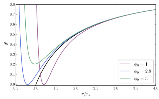
Figure 1: $g_{tt}$ component of the metric in the second branch of solutions, eq. (59), for $g_{1}=0,g_{3}=-2,g_{5}=1,M=1$. The black solid line shows the Schwarzschild solution. Although all the solutions are asymptotically flat, large deviations from Schwarzschild can exist near the horizon. The points where $g_{tt}=0$ correspond to divergences of the Ricci scalar.

$$h(r)= 1-\frac{2M}{r}\,,$$ (58)

$$f(r)= \left[\sqrt{1-\frac{2M}{r}}-g_{3}\phi_{0}\frac{M^{2}(M+r)+2r^{2}(M-r+\sqrt{r(r-2M)})}{10M^{2}r^{3}}+g_{5}\phi_{0}\frac{6M^{2}}{r^{6}}\right.$$

$$\left.+g_{6}\phi_{0}\frac{1050M^{6}+7M^{5}r+5M^{4}r^{2}+4M^{2}r^{3}(r+M)+8r^{5}(M-r+\sqrt{r(r-2M)})}{154M^{4}r^{6}}\right]^{2}\,\,,$$ (59)

where an integration constant has been used in order to ensure asymptotic flatness: $f\to 1$ as $r\to\infty$. For large $r$, $f(r)$ behaves as

$$f=1-\frac{2M}{r}-\frac{g_{3}\,\phi_{0}M^{2}}{4r^{4}}+\cdots\,.$$ (60)

Thus, this solution describes asymptotic corrections to the Schwarzschild metric that start at order $1/r^{4}$ at large distances. The profile of $f(r)$ is shown in Fig. 1 for fixed $g_{i}$ and varying $\phi_{0}$, with values justified below. In general, conditions on the $g_{i}$ have to be imposed in order to keep the geometry regular. First of all, the square roots in (59) introduce complex terms in the metric that are also reflected in the curvature invariants. These terms are removed by the condition

$$-20g_{6}\phi_{0}+77M^{2}g_{3}\phi_{0}+385M^{4}=0\,.$$ (61)

Another condition comes from examining the Ricci scalar. Using the equations of motion, $R$ can be written as

$$R=\frac{3M^{2}\left[r^{3}g_{3}+15r(8g_{5}+9g_{6})-12M(22g_{5}+25g_{6})\right]\phi_{0}}{r^{9}\sqrt{f}}\,.$$ (62)

Thus, it generally diverges when $f=0$. Analytically finding the zeros of $f$ is complicated. Numerically we find that, given a set of $g_{i}$’s, the position where $f=0$ can be controlled with $\phi_{0}$. For $\phi_{0}>0$, this position can be pushed to $r<2M$ if at least one of the $g_{i}$’s is negative.

An alternative argument is the following: since $f$ is always positive, $f^{\prime}$ must change sign when $f=0$. Asymptotically, $f^{\prime}>0$. At $r=2M$, $f^{\prime}$ takes the value

$$-\frac{3\left[271M^{2}g_{3}\phi_{0}+60g_{5}\phi_{0}+1155M^{4}\right]\left[215M^{2}g_{3}\phi_{0}+48g_{5}\phi_{0}+1155M^{4}\right]}{163840M^{9}}\,.$$ (63)

If $f^{\prime}>0$ at $r=2M$, this suggests (although does not guarantee) that $f\neq 0$ for every $r>2M$. Requiring that one of the factors above is negative can be seen as a condition on $\phi_{0}$, and requiring that $\phi_{0}$ is positive implies that at least one $g_{i}$ is negative. For the values of $M$ and $g_{i}$ used in Fig. 1, the first factor becomes negative when $\phi_{0}\gtrsim 2.39$, and the second factor becomes negative when $\phi_{0}\gtrsim 3.02$. This agrees with the behaviour observed in Fig. 1.

5 Conclusions

In this work we introduced a covariant scalar-tensor theory of gravity aimed to provide a new realisation of Hořava proposal for a power-counting renormalizable theory of gravity. Our construction spontaneously breaks Lorentz symmetry through a non-vanishing scalar profile, and it has the special feature of not propagating scalar excitations around a foliation of space-time corresponding to a unitary gauge for the scalar field. We proved this fact using a covariant ADM method, and we also discussed the result in terms of the symmetries of the system. The dynamical degree of freedom in this gauge is a spin two tensor mode with modified dispersion relations: its equations of motion contain two time and up to six spatial derivatives, potentially realising Hořava’s idea. Our scalar-tensor interactions are invariant under a specific symmetry acting on the metric, which might protect their structure, and are related with cuscuton [28] and cuscuta-Galileon [29, 30] theories. We analytically determined spherically symmetric solutions for our theory, showing that there exists a branch of stealth solutions physically equivalent to General Relativity configurations, also in the presence of matter fields.

We conclude stressing again parallelisms and differences with other frameworks. In our scenario Lorentz symmetry is spontaneously broken, instead of explicitly broken as in the original construction of [2, 3]. We start from covariant actions, whose structure (as the presence of $\sqrt{X}$ coefficients) leads to a time dependent scalar profile, and spontaneous breaking of Lorentz invariance, even around flat space. Interestingly, the structure of scalar-tensor couplings, derived from the application of our specific choice disformal transformation, is such that scalar excitations do not propagate in an unitary gauge for the scalar. Hence, we do not need to worry about the behaviour and possible strong coupling issues associated with an extra mode, which require delicate treatments or extra ingredients in the original theory (see e.g. [4, 11, 12, 13, 14, 38]).

Much work is left for the future. It would be important to study whether this system can lead to a theory of gravity renormalizable beyond power counting: the theory shares many similarities with the projectable version of Hořava gravity – which is known to be renormalizable [10] – with the advantage of being free of dangerous scalar excitations. Additional work is needed in order to fully understand the stability of the structure of our construction, and whether the symmetry (19) can prevent the danger that additional Lorentz-violating operators can be generated at the quantum level. At the phenomenological level, it would be interesting to study in general terms possible consequences of our construction for cosmology, and to include more general parity violating interactions as well, along the lines of [62]. We hope to report soon on these issues.

Acknowledgments

It is a pleasure to thank Marco Crisostomi, Emir Gumrukcuoglu, Maria Mylova and Sergey Sibiryakov for interesting discussions, an anonymous referee for many suggestions to improve our work, and Guillem Domènech for comments on the manuscript. We are partially supported by the STFC grant ST/P00055X/1.

Appendix A The expression for the disformed Lagrangians

The Lagrangian density $\tilde{\cal L}_{R^{(2)}}$ is given by

$$\tilde{\cal L}_{R^{(2)}}= g_{2}\,{\sqrt{\vphantom{X^{2}}X}}\left[\frac{2\left\langle\Phi^{2}\right\rangle}{X^{2}}+\frac{\left[\Phi^{2}\right]}{{X}}+{R}{}-\frac{2\langle\Phi\rangle([\Phi])}{X^{2}}-\frac{{[\Phi]}^{2}}{{X}}+\frac{2R^{\mu\nu}\partial_{\mu}\phi\partial_{\mu}\phi}{{X}}\right]^{2}$$

$$+g_{3}\,\sqrt{X}\,\bigg{[}\left[R^{2}\right]+\frac{2\langle R^{2}\rangle}{{X}}+R_{{\sigma\rho}}\left(\frac{2\Phi^{{\mu\rho}}\Phi_{\mu}^{\sigma}}{{X}}+\frac{2\langle R\rangle^{{\sigma\rho}}}{{X}}-\frac{2\Phi^{{\sigma\rho}}{[\Phi]}}{{X}}\right)+\frac{\left[\Phi^{4}\right]}{X^{2}}+\frac{{\langle R\rangle}^{2}}{X^{2}}$$

$$+\frac{4\langle R_{{\nu\rho}}\Phi_{\mu}^{\sigma}\Phi_{\sigma}^{\rho}\rangle}{X^{2}}+\langle R\rangle_{{\gamma\delta}}\left(\frac{\langle R\rangle^{{\gamma\delta}}}{X^{2}}+\frac{2\Phi^{{\sigma\delta}}\Phi_{\sigma}^{\gamma}}{X^{2}}-\frac{2\Phi^{{\gamma\delta}}{[\Phi]}}{X^{2}}\right)-\frac{2R_{{\gamma\delta}}\Phi^{{\gamma\delta}}\langle\Phi\rangle}{X^{2}}-\frac{2\left[\Phi^{3}\right]{[\Phi]}}{X^{2}}$$

$$-\frac{4\langle R_{{\nu\sigma}}\Phi_{\mu}^{\sigma}\rangle{[\Phi]}}{X^{2}}+\frac{2\langle R_{{\sigma\rho}}\Phi_{\mu}^{\sigma}\Phi_{\nu}^{\rho}\rangle}{X^{2}}+\frac{{[\Phi]}^{2}\left[\Phi^{2}\right]}{X^{2}}-\frac{6\left\langle\Phi^{3}\right\rangle{[\Phi]}}{X^{3}}+\frac{2\langle\langle R\rangle_{{\gamma\delta}}\Phi_{\mu}^{\gamma}\Phi_{\nu}^{\delta}\rangle}{X^{3}}+2\frac{\left[\Phi^{4}\right]+\langle\Phi^{4}\rangle}{X^{3}}$$

$$+\frac{2\left\langle\Phi^{2}\right\rangle{[\Phi]}^{2}}{X^{3}}+\frac{2\left\langle\Phi^{2}\right\rangle{\langle R\rangle}}{X^{3}}-\frac{2\langle R\rangle_{{\gamma\delta}}\Phi^{{\gamma\delta}}\langle\Phi\rangle}{X^{3}}-\frac{2\left[\Phi^{3}\right]\langle\Phi\rangle}{X^{3}}+\frac{2\left[\Phi^{2}\right]{[\Phi]}\langle\Phi\rangle}{X^{3}}-\frac{2{[\Phi]}{\langle R\rangle}\langle\Phi\rangle}{X^{3}}$$

$$-\frac{2\left\langle\Phi^{2}\right\rangle\langle\Phi\rangle}{X^{4}}-\frac{2\left\langle\Phi^{2}\right\rangle{[\Phi]}\langle\Phi\rangle}{X^{4}}+\frac{2\left\langle\Phi^{2}\right\rangle^{2}}{X^{4}}+\frac{\left[\Phi^{2}\right]\langle\Phi\rangle^{2}}{X^{4}}+\frac{{[\Phi]}^{2}\langle\Phi\rangle^{2}}{X^{4}}\bigg{]}\,.$$ (64)

Here, $\Phi$ is a matrix with components $\nabla^{\mu}\nabla_{\nu}\phi$, and

$$X =-\partial^{\mu}\phi\partial_{\mu}\phi\,,$$ (65)

$$[\Phi^{n}] =\text{tr}(\Phi^{n})\,,$$ (66)

$$\langle\Phi^{n}\rangle =\partial\phi\cdot\Phi^{n}\cdot\partial\phi\,,$$ (67)

$$\langle R\rangle_{\mu\nu} =\partial^{\alpha}\phi\partial^{\beta}\phi R_{\alpha\mu\beta\nu}\,,$$ (68)

and where indices are explicit, the free indices inside $\langle\ \rangle$ are contracted with two first derivatives of the scalar field.

Although the expressions for the disformal Lagrangians can be quite cumbersome, obtaining them is not a complicated task. The idea is simple: compute the Christoffel symbols for the disformal metric, and use these symbols to construct the geometric quantities of interest. The new Christoffel symbols $(\Gamma^{dis})^{\alpha}_{\mu\nu}$ are those of the original metric plus contributions from the scalar field. We can use this fact to simplify the calculations and express the new geometric quantities in terms of the old ones plus terms coming from the difference between the Christoffel symbols of $g_{\mu\nu}$ and of the disformal metric. For example, the transformed Riemann tensor is[20]

$$(R^{dis})^{\alpha}{}_{\beta\mu\nu}=R^{\alpha}{}_{\beta\mu\nu}+2\nabla_{[\mu}\mathcal{K}^{\alpha}{}_{\nu]\beta}+2\mathcal{K}^{\alpha}{}_{\gamma[\mu}\mathcal{K}^{\gamma}{}_{\nu]\beta}\,,$$ (69)

where, for the disformal transformation (5), $\mathcal{K}^{\alpha}{}_{\mu\nu}=(\Gamma^{dis})^{\alpha}_{\mu\nu}-\Gamma^{\alpha}_{\mu\nu}$ takes the form

$$\mathcal{K}^{\alpha}{}_{\mu\nu}=-\frac{\partial^{\alpha}\phi\nabla_{\mu}\partial_{\nu}\phi}{\epsilon^{2}-\partial^{\beta}\phi\partial_{\beta}\phi}\,.$$ (70)

With the help of symbolic computation packages such as xAct[63], it is straightforward to compute the contractions of the Riemann tensor required to obtain the disformal Lagrangians, being careful to transform also the covariant derivatives when necesseary, e.g. when computing the transformation of $\Box R$.

Appendix B Hamiltonian analysis

In this Appendix we develop a Hamiltonian analysis of a special case of our system, showing that it propagates only a spin-two degree of freedom in unitary gauge.

We focus on the Einstein-Hilbert action supplemented with the singular disformal transformation of the Ricci scalar, associated with Lagrangian (16). When expressed in unitary gauge and making use of a 3+1 ADM formalism, the action reads

$$S(\gamma,N,N^{i})=\int dtL=\int dt\,d^{3}x\sqrt{\gamma}N\left(\hat{R}+K_{ij}K^{ij}+K^{2}\right)+g_{1}\phi_{0}\sqrt{\gamma}\hat{R}\,$$ (71)

where we have ignored a boundary term from the Einstein-Hilbert part of the action. The dynamics (time derivatives) of the metric are contained only in the extrinsic curvature.

In order to write the Hamiltonian for (71), we have to compute the canonical momenta conjugated to $\gamma$, $N$, and $N^{i}$. Since no time derivatives of the lapse and shift functions appear in the action, the only non-vanishing momentum is

$$\tilde{P}^{ij}=\frac{\delta L}{\delta\dot{\gamma}_{ij}}=\sqrt{q}(K^{ij}-K\gamma^{ij})\,.$$ (72)

The time derivatives of the metric can be written in terms of the momenta, mod. the undetermined functions $N$ and $N^{i}$. Thus the Hamiltonian reads

$$H=\int d^{3}xN\left(-\sqrt{\gamma}\hat{R}+\frac{1}{\sqrt{\gamma}}\left(\tilde{P}^{ij}\tilde{P}_{ij}-\frac{1}{2}\tilde{P}^{2}\right)\right)-2N^{i}\gamma_{ij}D_{k}\tilde{P}^{jk}-g_{1}\phi_{0}\sqrt{\gamma}\hat{R}\,.$$ (73)

The lapse and shift functions play the role of Lagrange multipliers enforcing the constraints

$$P_{N} =-\sqrt{\gamma}\hat{R}+\frac{1}{\sqrt{\gamma}}\left(\tilde{P}^{ij}\tilde{P}_{ij}-\frac{1}{2}\tilde{P}^{2}\right)\approx 0\,,$$ (74)

$$P_{i} =-2\gamma_{ij}D_{k}\tilde{P}^{jk}\approx 0\,,$$ (75)

which define the constraint functions $C(N)=\int d^{3}xNP_{N}$ and $C(\vec{N})=\int d^{3}xN^{i}P_{i}$. Notice that these constraints are the same as in GR.

The Poisson bracket between two real functions, say $f$ and $g$, in phase space is given by

$$\left\{f,g\right\}=\int d^{3}x\frac{\delta f}{\delta\gamma_{ij}}\frac{\delta g}{\delta\tilde{P}^{ij}}-\frac{\delta f}{\delta\tilde{P}^{ij}}\frac{\delta g}{\delta\gamma_{ij}}$$ (76)

It is possible to verify that the constraint functions satisfy

$$\{C(\vec{N}),C(\vec{M})\} =C(\mathcal{L}_{N}M^{i})\,,$$ (77)

$$\{C(\vec{N}),C(M)\} =C(\mathcal{L}_{N}M)\,,$$ (78)

$$\{C(N),C(M)\} =C(\vec{K})\,,$$ (79)

where $K^{i}=\gamma^{ij}(N\partial_{j}M-M\partial_{j}N)$. This implies that the constraint functions form a first class set.

In contrast to GR, the total Hamiltonian is not only a sum of these first class constraints: it contains additional pieces proportional to $g_{i}$ – in the specific case we are considering here, the last term in eq.  (73). Thus, the fact that our first class constraints are the same as in GR does not automatically guarantee that they are preserved in time: additional constraints associated with this requirement can prevent the propagation of scalar degrees of freedom.

An interesting, general approach for directly discussing such conditions for preventing the propagation of scalar modes in unitary gauge has been developed in[64]. Their starting point is the following general structure for an action in ADM variables, where the extrinsic curvature is replaced by an auxiliary variable $Q_{ij}$ by means of Lagrange multipliers:

$$S=\int dtd^{3}x\,N\sqrt{\gamma}\left[L(t,N,\gamma_{ij},\hat{R}_{ij},Q_{ij})+v^{ij}(Q_{ij}-K_{ij})\right]\,.$$ (80)

Our action (71) can be easily expressed as above. The canonical momenta of (80) define a set of primary constraints, whose preservation in time defines a set of secondary constraints. The preservation in time of the secondary constraints leads to a linear system of equations that can usually be solved in terms of the Lagrange multipliers that enforce the primary constraints in the total Hamiltonian. However, if this is not possible due to degeneracy of the system, one then needs to impose further tertiary constraints, which reduce the number of propagating degrees of freedom. In the case of an action of the form eq. (80), such degeneracy condition reads (see [64] for full details):

$$\Delta\equiv(NL)_{NN}-NL^{ij}_{QN}(L^{-1}_{QQ})_{ij,kl}L^{kl}_{QN}=0\,,$$ (81)

where suffixes as $L_{N}$ etc mean derivatives of the Lagrangian along the fields in the index. It is straightforward to show that our Lagrangian satisfies this condition. Indeed, in our case the combination $NL$ is composed of two parts, one that depends linearly in $N$, and another one that does not depend on $N$, so that $L_{NN}=0$. We are then left to show that the second term in $\Delta$ vanishes: the additional terms in our Lagrangian do not depend on the extrinsic curvature and therefore do not depend either on the auxiliary variably $Q$, on the other hand, the GR part does not depend on $N$, thus $L_{NQ}=0$. In conclusion, the action (71) leads to the degeneracy condition $\Delta=0$, which implies the existence of a tertiary constraints forbidding the propagation of a scalar excitation in unitary gauge: our theory then propagates only a spin-2 mode when the scalar satisfies an unitary gauge.

A more direct way to reach the same result is to make use of the findings around (36), where we have seen that the identity (21) translates into the conservation of the constraints. Thus, the model we are considering here has the same number of initial degrees of freedom, and the same number and type of constraints as GR, therefore it propagates only two degrees of freedom.

Appendix C Spherically symmetric solutions with matter fields

In this Appendix we reconsider the first branch of spherically symmetric solutions discussed in Section 4.2, but we extend our arguments to consider an arbitrary matter sector minimally coupled to gravity. The action we consider is

$$S_{(g_{\mu\nu}+\phi+matter)}\,=\,\frac{M_{Pl}^{2}}{2}\,\int d^{4}x\,\sqrt{-g}\,R\,+\,\tilde{S}_{\phi}+\int d^{4}x\,\sqrt{-g}\,{\cal L}_{m}\,,$$ (82)

where $\tilde{S}_{\phi}$ is given in equation (14), and ${\cal L}_{m}$ a matter Lagrangian. We have learned in Section 4.2 that in absence of matter the theory admits a branch of spherically symmetric, stealth configurations which are physically equivalent to the solutions of Einstein gravity. Here we show that the same remains true also in presence of matter, as long as there are no direct couplings between matter and scalar field, as in eq (82). In other words, we show that there is a branch of configurations where the spherically symmetric solutions of (82) coincide with the ones of the reduced action

$$S_{(g_{\mu\nu}+matter)}\,=\,\frac{M_{Pl}^{2}}{2}\,\int d^{4}x\,\sqrt{-g}\,R\,+\,\int d^{4}x\,\sqrt{-g}\,{\cal L}_{m}\,.$$ (83)

This feature is not unique to our scalar-tensor theory, and has been recently proved to be shared with vector-tensor solutions [35] in vector-tensor theories of gravity first introduced in [59, 60, 61].

The argument goes as follow (see [35] for more details in a very similar set-up). One starts from a general static spherically symmetric Ansatz for the metric ,

$$ds^{2} =-f(r)dt^{2}+h(r)^{-1}dr^{2}+2k(r)dtdr+r^{2}(d\theta^{2}+\sin^{2}\theta)\,,$$ (84)

and a general spherically symmetric Ansatz for the scalar, $\phi(t,r)$. We derive the equations of motion for the metric components, and for the scalar field associated with action (82). We select a unitary gauge $\phi(t,r)\,=\,\phi_{0}t$ for the scalar profile, and choose an Ansatz $h(r)\,=\,1$ for one of the metric components: this profile for $h$ characterizes the stealth branch of solutions in vacuum, see eq (57). We find that the scalar field equation automatically vanishes, and the remaining equations for the metric components $f(r)$, $k(r)$ are completely independent of the scalar, and are the same equations one would derive from the action (83) by selecting the Ansatz $h(r)=1$. This implies that the spherically symmetric solutions are the same as in GR, as we wish to demonstrate. Within GR there is no preferred foliation, and one can choose a gauge different from $h=1$ by changing coordinates: nevertheless the physical properties of the solutions are the same in any coordinate system.

References

- [1] K. S. Stelle, “Renormalization of Higher Derivative Quantum Gravity,” Phys. Rev. D 16 (1977) 953. doi:10.1103/PhysRevD.16.953
- [2] P. Horava, “Membranes at Quantum Criticality,” JHEP 0903 (2009) 020 doi:10.1088/1126-6708/2009/03/020 [arXiv:0812.4287 [hep-th]].
- [3] P. Horava, “Quantum Gravity at a Lifshitz Point,” Phys. Rev. D 79 (2009) 084008 doi:10.1103/PhysRevD.79.084008 [arXiv:0901.3775 [hep-th]].
- [4] D. Blas, O. Pujolas and S. Sibiryakov, “On the Extra Mode and Inconsistency of Horava Gravity,” JHEP 0910 (2009) 029 doi:10.1088/1126-6708/2009/10/029 [arXiv:0906.3046 [hep-th]].
- [5] C. Charmousis, G. Niz, A. Padilla and P. M. Saffin, “Strong coupling in Horava gravity,” JHEP 0908 (2009) 070 doi:10.1088/1126-6708/2009/08/070 [arXiv:0905.2579 [hep-th]].
- [6] M. Li and Y. Pang, “A Trouble with Horava-Lifshitz Gravity,” JHEP 0908 (2009) 015 doi:10.1088/1126-6708/2009/08/015 [arXiv:0905.2751 [hep-th]].
- [7] D. Blas, O. Pujolas and S. Sibiryakov, “Consistent Extension of Horava Gravity,” Phys. Rev. Lett. 104 (2010) 181302 doi:10.1103/PhysRevLett.104.181302 [arXiv:0909.3525 [hep-th]].
- [8] D. Blas, O. Pujolas and S. Sibiryakov, “Models of non-relativistic quantum gravity: The Good, the bad and the healthy,” JHEP 1104 (2011) 018 doi:10.1007/JHEP04(2011)018 [arXiv:1007.3503 [hep-th]].
- [9] D. Blas and S. Sibiryakov, “Horava gravity versus thermodynamics: The Black hole case,” Phys. Rev. D 84 (2011) 124043 doi:10.1103/PhysRevD.84.124043 [arXiv:1110.2195 [hep-th]].
- [10] A. O. Barvinsky, D. Blas, M. Herrero-Valea, S. M. Sibiryakov and C. F. Steinwachs, “Renormalization of Horava gravity,” Phys. Rev. D 93 (2016) no.6, 064022 doi:10.1103/PhysRevD.93.064022 [arXiv:1512.02250 [hep-th]].
- [11] P. Horava and C. M. Melby-Thompson, “General Covariance in Quantum Gravity at a Lifshitz Point,” Phys. Rev. D 82 (2010) 064027 doi:10.1103/PhysRevD.82.064027 [arXiv:1007.2410 [hep-th]].
- [12] A. M. da Silva, “An Alternative Approach for General Covariant Horava-Lifshitz Gravity and Matter Coupling,” Class. Quant. Grav. 28 (2011) 055011 doi:10.1088/0264-9381/28/5/055011 [arXiv:1009.4885 [hep-th]].
- [13] Y. Huang and A. Wang, “Stability, ghost, and strong coupling in nonrelativistic general covariant theory of gravity with ,” Phys. Rev. D 83 (2011) 104012 doi:10.1103/PhysRevD.83.104012 [arXiv:1011.0739 [hep-th]].
- [14] T. Zhu, Q. Wu, A. Wang and F. W. Shu, Phys. Rev. D 84 (2011) 101502 doi:10.1103/PhysRevD.84.101502 [arXiv:1108.1237 [hep-th]]; T. Zhu, F. W. Shu, Q. Wu and A. Wang, Phys. Rev. D 85 (2012) 044053 doi:10.1103/PhysRevD.85.044053 [arXiv:1110.5106 [hep-th]]; K. Lin, S. Mukohyama, A. Wang and T. Zhu, Phys. Rev. D 89 (2014) no.8, 084022 doi:10.1103/PhysRevD.89.084022 [arXiv:1310.6666 [hep-ph]].
- [15] T. P. Sotiriou, “Horava-Lifshitz gravity: a status report,” J. Phys. Conf. Ser. 283 (2011) 012034 doi:10.1088/1742-6596/283/1/012034 [arXiv:1010.3218 [hep-th]].
- [16] S. Mukohyama, “Horava-Lifshitz Cosmology: A Review,” Class. Quant. Grav. 27 (2010) 223101 doi:10.1088/0264-9381/27/22/223101 [arXiv:1007.5199 [hep-th]].
- [17] A. Wang, “Horava gravity at a Lifshitz point: A progress report,” Int. J. Mod. Phys. D 26 (2017) no.07, 1730014 doi:10.1142/S0218271817300142 [arXiv:1701.06087 [gr-qc]].
- [18] J. D. Bekenstein, “The Relation between physical and gravitational geometry,” Phys. Rev. D 48 (1993) 3641 doi:10.1103/PhysRevD.48.3641 [gr-qc/9211017].
- [19] D. Bettoni and S. Liberati, “Disformal invariance of second order scalar-tensor theories: Framing the Horndeski action,” Phys. Rev. D 88 (2013) 084020 doi:10.1103/PhysRevD.88.084020 [arXiv:1306.6724 [gr-qc]].
- [20] M. Zumalacárregui and J. García-Bellido, “Transforming gravity: from derivative couplings to matter to second-order scalar-tensor theories beyond the Horndeski Lagrangian,” Phys. Rev. D 89 (2014) 064046 doi:10.1103/PhysRevD.89.064046 [arXiv:1308.4685 [gr-qc]].
- [21] M. Crisostomi, M. Hull, K. Koyama and G. Tasinato, JCAP 1603 (2016) no.03, 038 doi:10.1088/1475-7516/2016/03/038 [arXiv:1601.04658 [hep-th]].
- [22] J. Ben Achour, D. Langlois and K. Noui, “Degenerate higher order scalar-tensor theories beyond Horndeski and disformal transformations,” Phys. Rev. D 93 (2016) no.12, 124005 doi:10.1103/PhysRevD.93.124005 [arXiv:1602.08398 [gr-qc]].
- [23] J. Gleyzes, D. Langlois, F. Piazza and F. Vernizzi, “Healthy theories beyond Horndeski,” Phys. Rev. Lett. 114 (2015) no.21, 211101 doi:10.1103/PhysRevLett.114.211101 [arXiv:1404.6495 [hep-th]].
- [24] J. Gleyzes, D. Langlois, F. Piazza and F. Vernizzi, “Exploring gravitational theories beyond Horndeski,” JCAP 1502 (2015) 018 doi:10.1088/1475-7516/2015/02/018 [arXiv:1408.1952 [astro-ph.CO]].
- [25] D. Langlois and K. Noui, “Degenerate higher derivative theories beyond Horndeski: evading the Ostrogradski instability,” JCAP 1602 (2016) no.02, 034 doi:10.1088/1475-7516/2016/02/034 [arXiv:1510.06930 [gr-qc]].
- [26] M. Crisostomi, K. Koyama and G. Tasinato, “Extended Scalar-Tensor Theories of Gravity,” JCAP 1604 (2016) no.04, 044 doi:10.1088/1475-7516/2016/04/044 [arXiv:1602.03119 [hep-th]].
- [27] J. Ben Achour, M. Crisostomi, K. Koyama, D. Langlois, K. Noui and G. Tasinato, “Degenerate higher order scalar-tensor theories beyond Horndeski up to cubic order,” JHEP 1612 (2016) 100 doi:10.1007/JHEP12(2016)100 [arXiv:1608.08135 [hep-th]].
- [28] N. Afshordi, D. J. H. Chung and G. Geshnizjani, “Cuscuton: A Causal Field Theory with an Infinite Speed of Sound,” Phys. Rev. D 75 (2007) 083513 doi:10.1103/PhysRevD.75.083513 [hep-th/0609150].
- [29] J. Chagoya and G. Tasinato, “A geometrical approach to degenerate scalar-tensor theories,” JHEP 1702 (2017) 113 doi:10.1007/JHEP02(2017)113 [arXiv:1610.07980 [hep-th]].
- [30] C. de Rham and H. Motohashi, “Caustics for Spherical Waves,” Phys. Rev. D 95 (2017) no.6, 064008 doi:10.1103/PhysRevD.95.064008 [arXiv:1611.05038 [hep-th]].
- [31] M. Asorey, J. L. Lopez and I. L. Shapiro, Int. J. Mod. Phys. A 12 (1997) 5711 doi:10.1142/S0217751X97002991 [hep-th/9610006]; L. Modesto and I. L. Shapiro, Phys. Lett. B 755 (2016) 279 doi:10.1016/j.physletb.2016.02.021 [arXiv:1512.07600 [hep-th]].
- [32] J. Bhattacharyya, A. Coates, M. Colombo, A. E. Gumrukcuoglu and T. P. Sotiriou, “Revisiting the cuscuton as a Lorentz-violating gravity theory,” Phys. Rev. D 97 (2018) no.6, 064020 doi:10.1103/PhysRevD.97.064020 [arXiv:1612.01824 [hep-th]].
- [33] H. Gomes and D. C. Guariento, “Hamiltonian analysis of the cuscuton,” Phys. Rev. D 95 (2017) no.10, 104049 doi:10.1103/PhysRevD.95.104049 [arXiv:1703.08226 [gr-qc]].
- [34] F. Filippini and G. Tasinato, “An exact solution for a rotating black hole in modified gravity,” JCAP 1801 (2018) no.01, 033 doi:10.1088/1475-7516/2018/01/033 [arXiv:1709.02147 [hep-th]].
- [35] J. Chagoya and G. Tasinato, “Stealth configurations in vector-tensor theories of gravity,” JCAP 1801 (2018) no.01, 046 doi:10.1088/1475-7516/2018/01/046 [arXiv:1707.07951 [hep-th]].
- [36] C. de Rham and A. J. Tolley, “DBI and the Galileon reunited,” JCAP 1005 (2010) 015 doi:10.1088/1475-7516/2010/05/015 [arXiv:1003.5917 [hep-th]].
- [37] A. H. Chamseddine and V. Mukhanov, “Mimetic Dark Matter,” JHEP 1311 (2013) 135 doi:10.1007/JHEP11(2013)135 [arXiv:1308.5410 [astro-ph.CO]].
- [38] S. Nojiri and S. D. Odintsov, Phys. Rev. D 81 (2010) 043001 doi:10.1103/PhysRevD.81.043001 [arXiv:0905.4213 [hep-th]]; G. Cognola, R. Myrzakulov, L. Sebastiani, S. Vagnozzi and S. Zerbini, Class. Quant. Grav. 33 (2016) no.22, 225014 doi:10.1088/0264-9381/33/22/225014 [arXiv:1601.00102 [gr-qc]].
- [39] C. de Rham and A. Matas, “Ostrogradsky in Theories with Multiple Fields,” JCAP 1606 (2016) no.06, 041 doi:10.1088/1475-7516/2016/06/041 [arXiv:1604.08638 [hep-th]].
- [40] N. Afshordi, “Cuscuton and low energy limit of Horava-Lifshitz gravity,” Phys. Rev. D 80 (2009) 081502 doi:10.1103/PhysRevD.80.081502 [arXiv:0907.5201 [hep-th]].
- [41] D. Langlois and K. Noui, “Hamiltonian analysis of higher derivative scalar-tensor theories,” JCAP 1607 (2016) no.07, 016 doi:10.1088/1475-7516/2016/07/016 [arXiv:1512.06820 [gr-qc]].
- [42] S. Frittelli, “Note on the propagation of the constraints in standard (3+1) general relativity,” Phys. Rev. D 55 (1997) 5992. doi:10.1103/PhysRevD.55.5992
- [43] P. HAVAS, Rev. Mod. Phys. 36 (1964) 938. doi:10.1103/RevModPhys.36.938
- [44] T. Jacobson and D. Mattingly, “Gravity with a dynamical preferred frame,” Phys. Rev. D 64 (2001) 024028 doi:10.1103/PhysRevD.64.024028 [gr-qc/0007031].
- [45] D. Blas and E. Lim, “Phenomenology of theories of gravity without Lorentz invariance: the preferred frame case,” Int. J. Mod. Phys. D 23 (2015) 1443009 doi:10.1142/S0218271814430093 [arXiv:1412.4828 [gr-qc]].
- [46] N. Yunes, K. Yagi and F. Pretorius, “Theoretical Physics Implications of the Binary Black-Hole Mergers GW150914 and GW151226,” Phys. Rev. D 94 (2016) no.8, 084002 doi:10.1103/PhysRevD.94.084002 [arXiv:1603.08955 [gr-qc]].
- [47] A. Emir Gümrükçüoǧlu, M. Saravani and T. P. Sotiriou, “Hořava gravity after GW170817,” Phys. Rev. D 97 (2018) no.2, 024032 doi:10.1103/PhysRevD.97.024032 [arXiv:1711.08845 [gr-qc]].
- [48] S. Kiyota and K. Yamamoto, “Constraint on modified dispersion relations for gravitational waves from gravitational Cherenkov radiation,” Phys. Rev. D 92 (2015) no.10, 104036 doi:10.1103/PhysRevD.92.104036 [arXiv:1509.00610 [gr-qc]].
- [49] A. De Felice, D. Langlois, S. Mukohyama, K. Noui and A. Wang, “”Shadowy” modes in Higher-Order Scalar-Tensor theories,” arXiv:1803.06241 [hep-th].
- [50] E. Barausse, T. Jacobson and T. P. Sotiriou, “Black holes in Einstein-aether and Horava-Lifshitz gravity,” Phys. Rev. D 83 (2011) 124043 doi:10.1103/PhysRevD.83.124043 [arXiv:1104.2889 [gr-qc]].
- [51] E. Barausse and T. P. Sotiriou, “Black holes in Lorentz-violating gravity theories,” Class. Quant. Grav. 30 (2013) 244010 doi:10.1088/0264-9381/30/24/244010 [arXiv:1307.3359 [gr-qc]].
- [52] J. Maldacena, “Einstein Gravity from Conformal Gravity,” arXiv:1105.5632 [hep-th].
- [53] T. P. Sotiriou and S. Y. Zhou, “Black hole hair in generalized scalar-tensor gravity,” Phys. Rev. Lett. 112 (2014) 251102 doi:10.1103/PhysRevLett.112.251102 [arXiv:1312.3622 [gr-qc]].
- [54] T. P. Sotiriou and S. Y. Zhou, “Black hole hair in generalized scalar-tensor gravity: An explicit example,” Phys. Rev. D 90 (2014) 124063 doi:10.1103/PhysRevD.90.124063 [arXiv:1408.1698 [gr-qc]].
- [55] E. Babichev, C. Charmousis and A. Lehébel, “Asymptotically flat black holes in Horndeski theory and beyond,” JCAP 1704 (2017) no.04, 027 doi:10.1088/1475-7516/2017/04/027 [arXiv:1702.01938 [gr-qc]].
- [56] C. A. R. Herdeiro and E. Radu, “Asymptotically flat black holes with scalar hair: a review,” Int. J. Mod. Phys. D 24 (2015) no.09, 1542014 doi:10.1142/S0218271815420146 [arXiv:1504.08209 [gr-qc]].
- [57] T. P. Sotiriou, M. Visser and S. Weinfurtner, “Phenomenologically viable Lorentz-violating quantum gravity,” Phys. Rev. Lett. 102 (2009) 251601 doi:10.1103/PhysRevLett.102.251601 [arXiv:0904.4464 [hep-th]].
- [58] J. Greenwald, J. Lenells, J. X. Lu, V. H. Satheeshkumar and A. Wang, “Black holes and global structures of spherical spacetimes in Horava-Lifshitz theory,” Phys. Rev. D 84 (2011) 084040 doi:10.1103/PhysRevD.84.084040 [arXiv:1105.4259 [hep-th]].
- [59] G. Tasinato, “Cosmic Acceleration from Abelian Symmetry Breaking,” JHEP 1404 (2014) 067 doi:10.1007/JHEP04(2014)067 [arXiv:1402.6450 [hep-th]]
- [60] L. Heisenberg, “Generalization of the Proca Action,” JCAP 1405 (2014) 015 doi:10.1088/1475-7516/2014/05/015 [arXiv:1402.7026 [hep-th]].
- [61] G. Tasinato, “A small cosmological constant from Abelian symmetry breaking,” Class. Quant. Grav. 31 (2014) 225004 doi:10.1088/0264-9381/31/22/225004 [arXiv:1404.4883 [hep-th]].
- [62] M. Crisostomi, K. Noui, C. Charmousis and D. Langlois, “Beyond Lovelock gravity: Higher derivative metric theories,” Phys. Rev. D 97 (2018) no.4, 044034 doi:10.1103/PhysRevD.97.044034 [arXiv:1710.04531 [hep-th]].
- [63] http://www.xact.es
- [64] A. Iyonaga, K. Takahashi and T. Kobayashi, “Extended Cuscuton: Formulation,” arXiv:1809.10935 [gr-qc].
- [65]