Viscosity and self-diffusion of supercooled and stretched water from molecular dynamics simulations
Abstract
Among the numerous anomalies of water, the acceleration of dynamics under pressure is particularly puzzling. Whereas the diffusivity anomaly observed in experiments has been reproduced in several computer studies, the parallel viscosity anomaly has received less attention. Here we simulate viscosity and self-diffusion coefficient of the TIP4P/2005 water model over a broad temperature and pressure range. We reproduce the experimental behavior, and find additional anomalies at negative pressure. The anomalous effect of pressure on dynamic properties becomes more pronounced upon cooling, reaching two orders of magnitude for viscosity at . We analyze our results with a dynamic extension of a thermodynamic two-state model, an approach which has proved successful in describing experimental data. Water is regarded as a mixture of interconverting species with contrasting dynamic behaviors, one being strong (Arrhenius), and the other fragile (non-Arrhenius). The dynamic parameters of the two-state models are remarkably close between experiment and simulations. The larger pressure range accessible to simulations suggests a modification of the dynamic two-state model, which in turn also improves the agreement with experimental data. Furthermore, our simulations demonstrate the decoupling between viscosity and self-diffusion coefficient as a function of temperature . The Stokes-Einstein relation, which predicts a constant , is violated when is lowered, in connection with the Widom line defined by an equal fraction of the two interconverting species. These results provide a unifying picture of thermodynamics and dynamics in water, and call for experiments at negative pressure.
I Introduction
Liquid water exhibits countless thermodynamic and dynamic peculiarities Gallo et al. (2016). Among thermodynamic properties, well known anomalies are the negative expansion coefficient below at ambient pressure, or the rapid increase in isothermal compressibility and isobaric heat capacity upon cooling. These anomalies become more pronounced in supercooled water Debenedetti (2003); Holten et al. (2012). Several dynamic properties are also anomalous, showing a non-monotonic pressure dependence. Below room temperature, the shear viscosity reaches a minimum as a function of pressure Röntgen (1884); Warburg and Sachs (1884); Bridgman (1925); Bett and Cappi (1965), whose location has been recently tracked down to and , where is reduced by 42% compared to its value at ambient pressure Singh, Issenmann, and Caupin (2017). Diffusivity reaches a maximum as a function of pressure, which has been measured in supercooled water both for translation Prielmeier et al. (1988); Harris and Newitt (1997) and rotation Lang and Lüdemann (1981); Arnold and Lüdemann (2002). Stretched water, or water at negative pressure, has also been studied, although less extensively (see Ref. Caupin, 2015 for a review). The temperature of maximum density increases from at ambient pressure to at , and a maximum in the isothermal compressibility of water along isobars has been revealed around and below Holten et al. (2017).
A limit to experiments on metastable water is homogeneous nucleation of ice in supercooled water, or of vapor in stretched water. At deeply metastable conditions, nucleation becomes unavoidable on the timescale needed to perform measurements. Because of the small sizes and short timescales involved, molecular dynamics (MD) simulations provide a powerful alternative to experiments for studying physical properties at even more extreme conditions. Extensive thermodynamic data are already available for several water models such as ST2 Poole et al. (1992); Poole, Saika-Voivod, and Sciortino (2005) and TIP4P/2005 Agarwal, Alam, and Chakravarty (2011); González et al. (2016); Biddle et al. (2017). The self-diffusion coefficient has also been studied in simulations. Early simulations reproduced qualitatively the experimental behavior of : first its anomalous density dependence for ST2 Sciortino, Geiger, and Stanley (1991) and SPC/E water Vaisman, Perera, and Berkowitz (1993), and later its maximum for SPC/E water Starr, Sciortino, and Stanley (1999); Scala et al. (2000); Errington and Debenedetti (2001). A minimum in at low density, not yet observed in experiments, has also been found in simulations of TIP4P Ruocco et al. (1993) and SPC/E water Starr, Sciortino, and Stanley (1999); Errington and Debenedetti (2001); Netz et al. (2001). Agarwal et al. Agarwal, Alam, and Chakravarty (2011) simulated of water for five models, namely SPC/E, mTIP3P, TIP4P, TIP5P, and TIP4P/2005. Although they all show a maximum in as a function of density at low enough temperature, only TIP4P/2005 gives a maximum at ambient temperature, as observed in experiments. All models give rise to a minimum in at low density. One concern about the results for is the possible existence of finite-size effects, with simulations involving for instance 256 molecules only Agarwal, Alam, and Chakravarty (2011). Correcting for these effects requires the knowledge of the viscosity Yeh and Hummer (2004); Tazi et al. (2012).
However, simulations of viscosity are scarce. Because of its lower computational cost, the structural relaxation time is often used as a proxy for , as these two quantities are assumed to be proportional. However, Shi et al. Shi, Debenedetti, and Stillinger (2013) found that, for model atomic and molecular systems, is temperature dependent. The same issue was observed for a water model Guillaud et al. (2017a, b). Coming back to direct simulations of , we list here the important works relevant to our study. A minimum in the density dependence of was obtained with TIP4P/2005 González and Abascal (2010) and BK3 water Kiss and Baranyai (2014). Values of and for TIP4P/2005 were also reported Guevara-Carrion, Vrabec, and Hasse (2011) in the range – and –, and showed the maximum in , whereas the minimum in was hidden by the simulation uncertainties. To our knowledge, simulation data for of TIP4P/2005 water at supercooled conditions are only available at ambient pressure Guillaud et al. (2017a) or a density of . Kawasaki and Kim (2017) We are aware of only two simulation studies of viscosity in the supercooled region under pressure. The first by Dhabal et al. Dhabal et al. (2016) reported and for the coarse-grained mW model (monatomic water), and the density dependence gave a minimum and a maximum for and a minimum for . However, because it omits the reorientation of hydrogen atoms, mW gives three times higher and three times lower than experimental values for water at ambient conditions. The second study simulated the more realistic WAIL potential Ma, Li, and Wang (2015), but the pressure range investigated (–) precluded the observation of a minimum in .
It is therefore of interest to perform simulations with a realistic water model, aimed at the direct determination of in a broad pressure and temperature range. In particular, it should be possible to follow in the supercooled region the minimum in seen at stable conditions, and also to investigate if there is a maximum in at low density, similar to the second extremum seen in simulations of . In the present work, we have performed such simulations with TIP4P/2005 water. We have computed and at the same state points, so that we were able at the same time to apply finite-size corrections to .
An additional motivation of our work is to investigate the connection between thermodynamics and dynamics. In the case of real water, several works have addressed this question using a two-state model for theoretical frame Vedamuthu, Singh, and Robinson (1994); Cho, Urquidi, and Robinson (1999); Cho et al. (2002); Tanaka (2000, 2003). In Ref. Singh, Issenmann, and Caupin, 2017, an accurate thermodynamic two-state model Holten, Sengers, and Anisimov (2014) was successfully extended to describe dynamic data. As a similar thermodynamic two-state model is available for TIP4P/2005 water Biddle et al. (2017), we investigate here if its dynamic extension can also reproduce our simulated dynamic properties.
Finally, obtaining simultaneous data on and is also useful to test their coupling. Indeed, in liquids at high temperature, and are usually linked by the Stokes-Einstein (SE) relation, inspired by macroscopic hydrodynamics and linear response theory, which states that is independent of temperature. Deviations are observed in supercooled liquids, usually around 1.3 where is the glass transition temperature; see for instance Ref. Chang and Sillescu, 1997 for vs. for six glassformers. In contrast, at ambient pressure, water already exhibits a violation of the SE relation at room temperature (above ); this violation increases upon cooling, with a relative deviation around 70% at Dehaoui, Issenmann, and Caupin (2015). Understanding the origin of this early SE violation in water is an active field of research Guillaud et al. (2017a); Galamba (2017); Kawasaki and Kim (2017), as for other anomalies of water that become more pronounced in the supercooled region Gallo et al. (2016).
II Methods
| Simulations | Experiment | ||||
|---|---|---|---|---|---|
| Quantity | Viscosity | Self-diffusion | Viscosity | Self-diffusion | Rotational |
| coefficient | coefficient | correlation time | |||
II.1 Simulation details
We have selected the TIP4P/2005 model for water Abascal and Vega (2005), which is currently one of the best force fields available, describing nearly quantitatively many properties of water in a broad temperature and pressure range. Many thermodymanic quantities are available for TIP4P/2005 water, and they have been successfully described within the two-state formalism by Biddle et al. Biddle et al. (2017) (see Section II.2). We have performed runs of TIP4P/2005 water simulated via the LAMMPS MD package Plimpton (1995). is set to 216 molecules and the temperature is kept constant via a Nosé-Hoover thermostat. To remain consistent with the definition of TIP4P/2005 Abascal and Vega (2005), we used a cutoff. Long-range Coulombic interactions were computed using the particle-particle particle-mesh method Hockney and Eastwood (1988), and water molecules were held rigid using the SHAKE algorithm Ryckaert, Ciccotti, and Berendsen (1977). We simulate temperatures ranging from to and densities from to . We selected state points on a grid in the temperature-density plane, which includes the validity region of the thermodynamic two-state model by Biddle et al. Biddle et al. (2017). All state points have been simulated far beyond their characteristic time to ensure equilibration (see for instance Fig. 1B of Ref. 35 for characteristic times of TIP4P/2005 water at ). The run durations range from at and to at and ; at and , a longer duration of was used. For each state point, we obtain the shear viscosity by averaging the five independent Green-Kubo integrals of the auto-correlation function of traceless stress tensor elements Chen, Smit, and Bell (2009). As these calculations were computationally expensive, optimized algorithms were used Ramírez et al. (2010). We calculate the self-diffusion coefficient from the slope of the linear regression of the mean squared displacement in the diffusive regime. The slope is divided by 6 following the Einstein relation Allen and Tildesley (2017): to obtain (note that center of mass corrections have been used). Because of hydrodynamic interactions between image boxes in a simulation with periodic boundary conditions, the raw value of suffers from finite size effects. It has been shown on theoretical grounds and verified with simulations of boxes with different sizes Yeh and Hummer (2004); Tazi et al. (2012), that the value for the self-diffusion in an infinite liquid can be calculated with the following formula:
| (1) |
where is the self-diffusion coefficient before finite size correction (that is in a cubic simulation box of side with periodic boundary conditions), the Boltzmann constant, the temperature, and the viscosity (previously obtained from the simulation). Tazi et al. Tazi et al. (2012) also simulated TIP4P/2005 water but for only one state point. They computed for several box sizes , and used Eq. 1 to calculate for the infinite liquid. From the slope of vs. , they also obtained an estimate of , which was in perfect agreement with directly calculated from the Green-Kubo integrals. This validates our procedure of first calculating from the Green-Kubo integrals and for one value of (e.g. for ), and then using and Eq. 1 to calculate for the infinite liquid. Appendix A gives all simulations results for (Table 3) and for (Table 4). We also present in Appendix A how uncertainties on and were estimated; their values are given in the tables.
II.2 Two-state model
Two-state models are popular explanations of the anomalies of water, because anomalous behavior in such models stems from the variation of the fraction of each state, each having otherwise a normal behavior. For instance, Robinson and his colleagues provided a two-state description of density at ambient pressure Vedamuthu, Singh, and Robinson (1994), later extended to the pressure dependence of viscosity Cho, Urquidi, and Robinson (1999) and density Cho et al. (2002). A more comprehensive description was formulated by Tanaka Tanaka (2000, 2003) to account for the anomalous behavior of density, isothermal compressibility, isobaric heat capacity, and shear viscosity with a mixture of two states with fractions and . The dynamic part of Tanaka’s model describes the viscosity of water as a thermally activated process, whose activation energy is the fraction-weighted average of the activation energy for each state, and : . In other words, the hypothetic liquids made of each pure state would have an Arrhenius behavior (constant and ), and the non-Arrhenius behavior of real water would arise from the variation of the fraction . Holten, Sengers and Anisimov Holten, Sengers, and Anisimov (2014) developed an equation of state for water based on the two-state picture (HSA model). In the HSA model, water is considered as an athermal non-ideal ‘solution’ of two rapidly inter-convertible states or structures: a low density state (LDS) and a high density state (HDS), with respective fractions and . The non-ideality of the solution drives a first-order phase transition between two distinct liquids at low temperature, ending at a liquid-liquid critical point (LLCP) at and . We emphasize that there is currently no firmly established experimental proof of such a liquid-liquid transition and LLCP for real water, the main reason being that, in experiments, ice nucleates before reaching the putative two-phase region Caupin (2015). Nevertheless, the HSA model achieves a fit within experimental error of a comprehensive data set of thermodynamic properties (density, isothermal compressibility, thermal expansion coefficient, isobaric heat capacity, and speed of sound) in the range 200 to and 0.1 to . This equation of state is the current official guideline on thermodynamic properties of supercooled water {The International Association for the Properties of Water and Steam} (2015). Following Tanaka’s example Tanaka (2000, 2003), the HSA model was recently extended to dynamic properties by Singh et al. Singh, Issenmann, and Caupin (2017), who additionally measured viscosity of supercooled water under pressure. Experimental data for stable and supercooled water below and between and were included, not only for shear viscosity as Tanaka did Tanaka (2000, 2003), but also for self-diffusion coefficientPrielmeier et al. (1988); Harris and Newitt (1997) and rotational correlation time Lang and Lüdemann (1981); Arnold and Lüdemann (2002). It was observed that a mixture of two liquids following Arrhenius dynamics did not give satisfactory results. Instead, all properties could be reproduced within experimental uncertainty if the high density state was assumed to follow a fragile behavior. Eventually the following form was used to describe all three dynamic properties:
| (2) |
Here (introduced to make dimensionless), accounts for the temperature variation of the average speed of the molecules Prielmeier et al. (1988) ( for or , for 111The value of for is chosen for consistency with the Stokes-Einstein-Debye relation , which holds at high temperature, similar to the Stokes-Einstein relation Dehaoui, Issenmann, and Caupin (2015).), and for or and for . There are also 5 free parameters, as for Tanaka’s viscosity model. Their physical meaning is as follows. is a global scale factor. LDS behaves like an Arrhenian liquid with activation energy , whereas HDS behaves like a fragile liquid described by a Vogel-Tamann-Fulcher (VTF) law with parameters and . The energy appearing in the VTF law has a pressure dependence coming from the difference in volume between the activated and initial state of the activated process Tanaka (2000). A good fit, with good reduced and residuals, could be obtained holding equal for the three properties (see Fig. 3 of Ref. Singh, Issenmann, and Caupin, 2017). The best fit parameters are reproduced in Table 1. They are relatively close between properties, and have reasonable physical values. In particular, is of the order of the hydrogen bond energy, and is around 5-8% of the volume per molecule, around at .
One focus of the present paper is applying a two-state approach for simulation data. Recently, a set of thermodynamic properties of TIP4P/2005 water was successfully described with a two-state model similar to the HSA model Biddle et al. (2017). Its validity region (Fig. 1 of Ref. Biddle et al., 2017) covers temperatures from to and pressures from around to . It predicts a liquid-liquid critical point at and . These values are close to previous estimates for TIP4P/2005 Abascal and Vega (2010); Sumi and Sekino (2013); Yagasaki, Matsumoto, and Tanaka (2014); Singh et al. (2016). Although the existence of such a critical point in TIP4P/2005 has been challenged Overduin and Patey (2015), a recent approach based on potential energy landscape Handle and Sciortino (2018) also predicts a critical point. Inspired by the analysis performed on experimental data Singh, Issenmann, and Caupin (2017), we have investigated if, for simulations, the two-state model presented in Ref. Biddle et al., 2017 could be extended to describe dynamic properties.
III Results and discussion
III.1 Simulation results
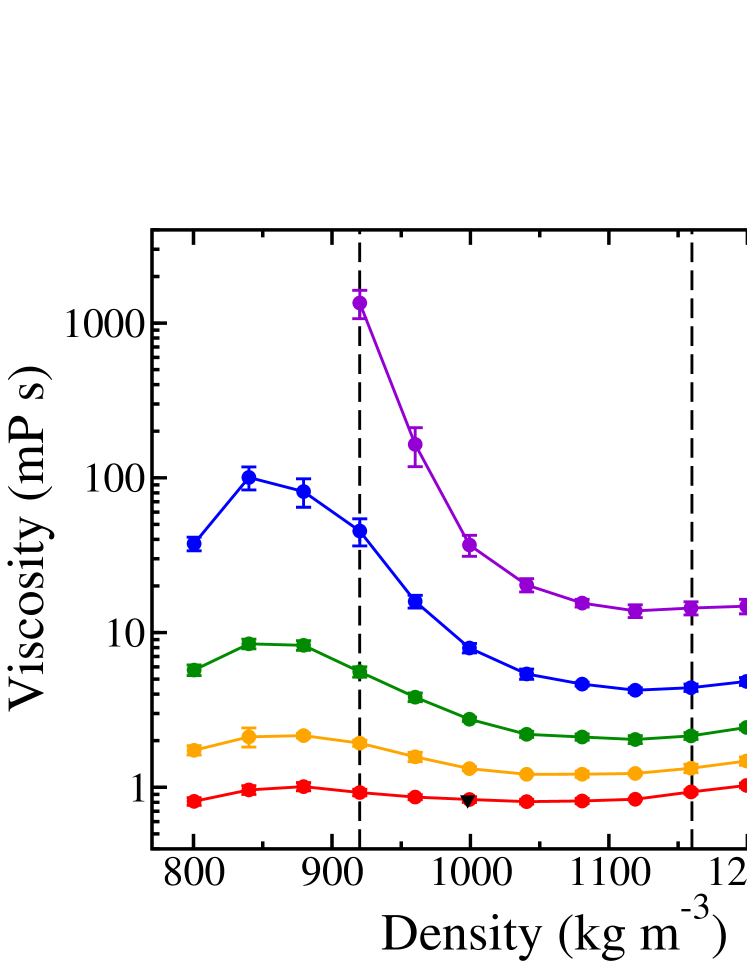
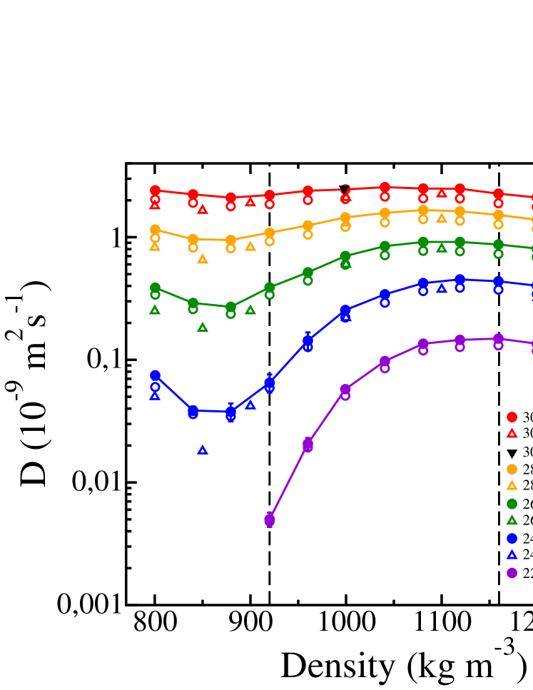
Figure 1 shows the final results for and as a function of density for a series of isotherms. Our results compare well with those of Tazi et al. Tazi et al. (2012) for both and . Our uncorrected values for agree well with Agarwal et al. Agarwal, Alam, and Chakravarty (2011) at high density. A slight discrepancy appears at low density and gets more pronounced at low temperature. Note that the difference with Ref. Agarwal, Alam, and Chakravarty (2011) is that we could correct for finite size effects because we have both and . Figure 2 shows a close-up, to allow comparison with experimental data. The fits of Ref. Singh, Issenmann, and Caupin, 2017 were used to represent the experimental data. Simulations reproduce well the fast temperature variation of and , together with their minimum and maximum as a function of density, respectively. This illustrates once more the good performance of the TIP4P/2005 model in reproducing the properties of experimental water. At lower densities, where no experiment are available at present, our simulations yield a maximum in versus and a minimum in versus . The minimum in has been previously observed in simulations Ruocco et al. (1993); Starr, Sciortino, and Stanley (1999); Errington and Debenedetti (2001); Netz et al. (2001); Agarwal, Alam, and Chakravarty (2011); Dhabal et al. (2016). To our knowledge, the maximum in is found here for the first time. The anomalous density variation (decrease of and increase of ) at fixed temperature becomes more pronounced upon cooling, as observed in the experiment (Fig. 2). The anomalous change measured experimentally corresponds to a maximum factor for at Singh, Issenmann, and Caupin (2017) and for at Prielmeier et al. (1988). Because the simulations reach lower temperatures and densities, the observed factors reach larger values. At , the anomalous change corresponds to a factor for and for ; note that these values are lower bounds, as no low density extremum is present in the density range of our simulations at this temperature.
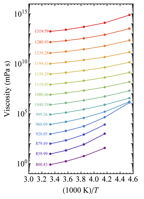
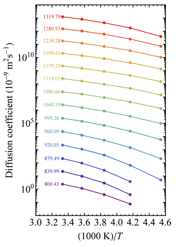
To illustrate the fragile character of TIP4P/2005 water, Appendix B shows the variation of and with inverse temperature in a log-lin plot for each isochore (Arrhenius plots). Arrhenius behavior would correspond to straight lines. Instead, the curves exhibit a more rapid variation with decreasing temperature. The effect tends to be more pronounced at lower densities.
III.2 Two-state analysis
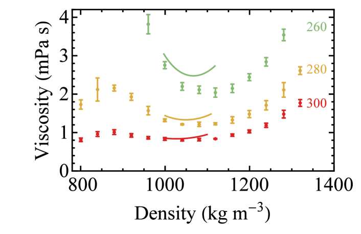
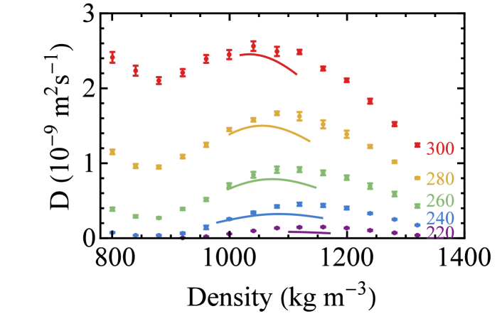
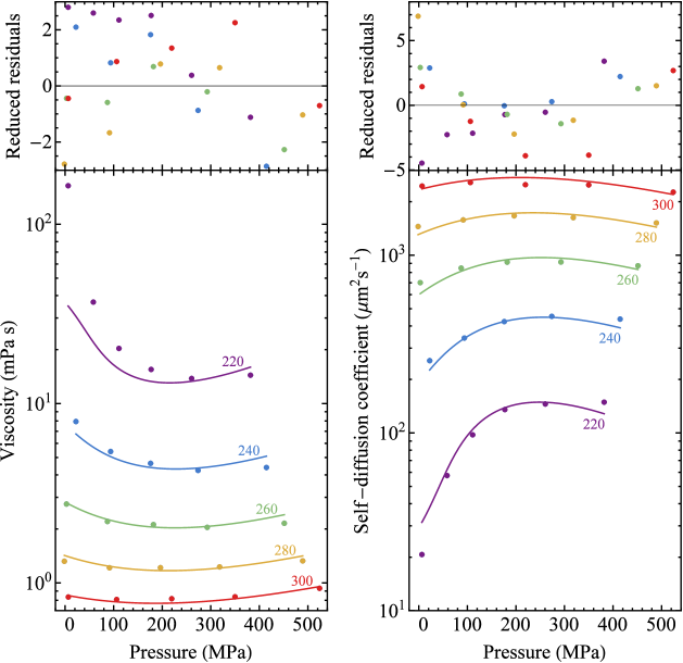
The analysis of the simulation data with the two-state model Biddle et al. (2017) presented in Section II.2 can be done only for state points in the validity region of the two-state model (between dashed vertical lines in Fig. 1). Therefore, only data with density between and were considered. Because the dynamic two-state model (Eq. 2) uses pressure as a variable, the pressure for each state point was calculated from its temperature and density, using the thermodynamic two-state model Biddle et al. (2017). As a first step, we have tried to reproduce the analysis of experimental data (see Section II.2). To this end, we have selected a subset of simulation data, set 1, at positive pressure as in the experiment. Because its pressure was very close to zero, we also included in set 1 a data point at and . The fit to Eq. 2 and the corresponding residuals are shown in Fig. 3, which corresponds to the simulation equivalent of Fig. 3 of Ref. Singh, Issenmann, and Caupin, 2017 for the experiments. Overall the fit quality is reasonable. The reduced residuals, defined as the difference between data and fit values divided by the data uncertainty, are acceptable, but a systematic deviation appears at low temperature and low density. Table 1 gives the best fit parameters. It can be seen that, as noted in Ref. Singh, Issenmann, and Caupin, 2017 for the experiment, and here as well for the simulation set 1, the values of , , and are in the same range for the different dynamic quantities. Note that they cannot have a common value for all dynamic properties, otherwise the SE relation would always hold. Moreover, the best fit parameters for the same dynamic quantity have similar values in simulations and in experiment. This confirms the good performance of the TIP4P/2005 model in reproducing the properties of experimental water. Remarkably, both in simulations and in experiment, the temperature is around , and is in the range –, the typical energy of a hydrogen bond. The activation volume is in the range –. This is around –% of the volume per molecule in the liquid, around at .
| Simulations | Experiment | ||||
|---|---|---|---|---|---|
| Quantity | Viscosity | Self-diffusion | Viscosity | Self-diffusion | Rotational |
| coefficient | coefficient | correlation time | |||
As a second step, we attempted to fit all simulation data belonging to the validity region of the two-state model Biddle et al. (2017). The fit to Eq. 2 deteriorates gradually when simulation data with lower density are successively added. Eq. 2 cannot generate a low-density extremum in dynamic quantities. Fig. 1 shows that these extrema lie outside the region of validity of the two-state model Biddle et al. (2017), but still their vicinity might be responsible for the discrepancy. To improve the fit, we tried a number of other formulas, obtained by making simple changes to Eq. 2. In all our attempts, one point at and , at the corner of the validity region, caused too large deviations, resulting in a reduced for and for for our best fit with a modified equation. Yet this state point was well equilibrated, as we checked by performing a -long simulation run. To keep the change to Eq. 2 to a minimum, we decided to discard this problematic point. We kept all other points in the region of validity of the two-state model Biddle et al. (2017) to form a second set of simulation data, set 2.
We were able to improve the fit to set 2 by adding a volume term in the activation energy for the LDS (similar to for the HDS), namely:
| (3) |
An advantage of Eq. 3 over Eq. 2 is that the former is able to yield a second extremum at low density. This can be understood by studying the derivative of with respect to pressure:
| (4) |
At high pressure, and , so that the dynamic behavior is normal, tending towards that of a pure HDS liquid. At intermediate pressures, the term has a sign opposite to the others, and, if its amplitude is sufficient (i.e. at low enough temperature), it causes the anomalous behavior of dynamic properties. When the pressure is sufficiently reduced, the term can dominate, causing the dynamic properties to recover a normal behavior.
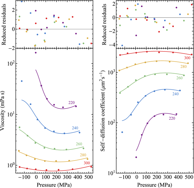
The fit to Eq. 3 and the corresponding residuals are shown in Fig. 4. The fit is good, with significantly better quality than the fit of set 1 to Eq. 2. The residuals are reasonable, although some bias remains at low temperature and at the two lowest densities. There are several possible reasons for this discrepancy, and for our need to discard the point at and . The simple linear pressure dependence of the apparent activation energies in Eq. 3 might not be sufficient for the large pressure range investigated; or some parameters of the thermodynamic two-state model (e.g. the location of the Widom line) might have to be modified, to improve the agreement with the dynamic data, without deteriorating the description of thermodynamic data. A simultaneous fit of both types of data is an interesting direction for future work.
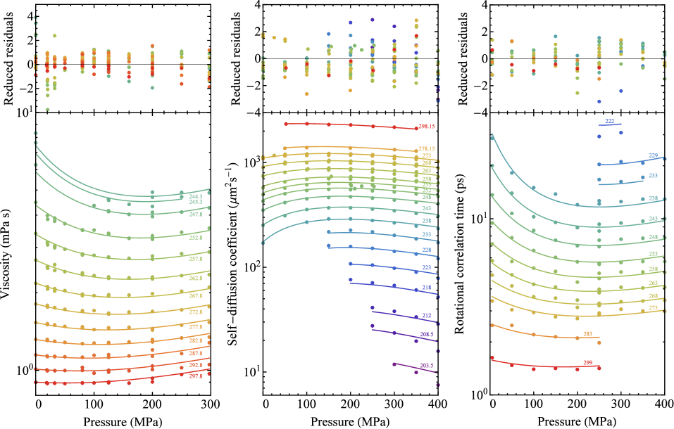
For comparison, we also performed the fit of experimental data to Eq. 3, as shown in Fig. 5. Table 2 gives the best fit parameters. Adding the term also improves the fit to experiment, albeit only slightly, presumably because of the restricted pressure interval and small values of the LDS fraction in the experimentally covered range. The values of , , , and are in the same range for the different dynamic quantities. , in the range –, still has the order of the energy of a hydrogen bond, whereas , , and are more different between simulations and experiment. is nearly the same as for the previous fit of the experimental data, whereas it is increased to for the fit of MD data. The activation volume is slightly increased but remains small, while the activation volume is rather large, in the range –. This value is similar to the volume per molecule in the liquid. In the model we propose, transport by a molecule in the LDS state would thus involve a considerable change in volume for the activated state. This is not unlikely, as the LDS state is sometimes viewed as a structure involving a tetrahedral arrangement of hydrogen bonded molecules, with low entropy and large volume.
We now discuss the value of appearing in the VTF-like behavior of the dynamics of the HDS state, Eqs. 2 and 3. , at which the system would be arrested, has been related to the Kauzmann temperature Adam and Gibbs (1965) or the mode-coupling temperature Gotze (1998). In the former case, it is expected to be lower than , whereas in the latter case, should be higher than , because of hopping processes. for water has been reported below Loerting et al. (2015). However, a recent comparison of the calorimetric features of the glass phases of several water isotopes Shephard and Salzmann (2016) points towards a reinterpretation of the glass transition as an orientational glass transition. The true structural glass transition of water might therefore occur at temperature above , which eludes observation because of crystallization upon further heating. We make the conservative statement that the best fit value for is close to .
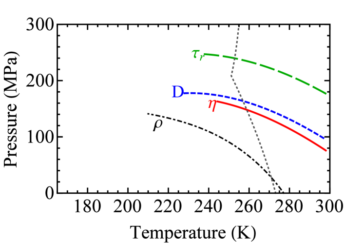
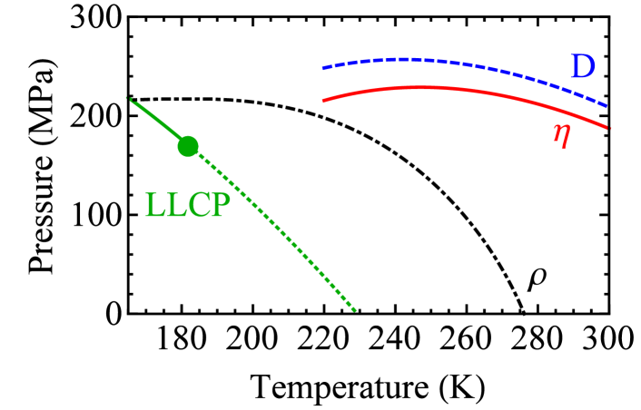
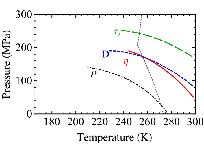
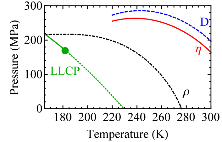
Finally, we compare the lines of extrema for experiment and simulations, as derived from the fitting of experiment and simulation set 1 to Eq. 2 (Fig. 6), and of experiment and simulation set 2 to Eq. 3 (Fig. 7). The line of density maxima is also shown, together with the liquid-liquid transition and the Widom line for TIP4P/2005. All figures are qualitatively similar. We note that Fig. 6 does not show the intersection between the line of minima in and of maxima in for the fit to experiment, nor the maxima of these lines for the fit to simulations, which can be seen in Fig. 7. We believe that these features are not significant, and rather due to inaccuracies of the fit in locating the rather shallow extrema (see Figs. 3 to 5). A robust result is the nested pattern formed by the lines. Part of this pattern was observed in previous simulations Errington and Debenedetti (2001); Poole et al. (2011); Nayar and Chakravarty (2013), with the locus of maxima in encircling the line of density maxima. The same arrangement of these lines was also observed for mW water, with in addition the locus of minima in located in between them. However, mW does not reproduce quantitatively the dynamics of real water (see Section I). Here, with the more quantitative TIP4P/2005 water model, we find the lines of extrema in the same order as, and at a location close to, the experimental lines of extrema.
III.3 Stokes-Einstein relation
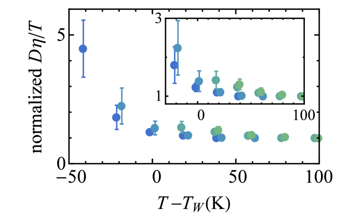
We are now in a position to test the SE relation by combining the simulation results. We choose to use directly the raw simulation data rather than the fits presented in Section III.2, because the simulations cover a larger range of temperature and pressure. Moreover, in their validity region, the fits exhibit systematic deviations which, although small for the absolute values of and compared to the simulation uncertainties, result in an excessive underestimate of the product . To emphasize the temperature variation, is usually normalized at a reference temperature, which is taken as in Fig. 8. For , the violation reaches 24% at , which is comparable to the violation of around 60% observed in the experiment at and atmospheric pressure. At a given temperature, the SE violation tends to become more pronounced at lower densities; however, the density dependence is not monotonic.
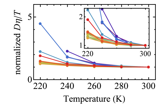
Kumar et al. Kumar et al. (2007) studied the SE relation for two other models of water: TIP5P and ST2. Note that they used the structural relaxation time as a proxy for the shear viscosity (see Section I). They related the violation of SE to the existence of a LLCP in the supercooled liquid, and more particularly to the Widom line emanating from this LLCP, located at a temperature function of the pressure . They found that, at pressures lower than the LLCP pressure, the curves for each pressure collapsed onto a master curve when plotted as a function of the distance to the Widom line, , instead of the temperature. We have tested this collapse. Strictly speaking, the Widom line is the locus of correlation length maxima associated with the LLCP. As a proxy for , Kumar et al. used the maxima of isobaric heat capacity along isobars, which asymptotically approaches the Widom line near the LLCP. Here instead, we use the two-state model presented in Section II.2. For the 4 isochores having a density below the LLCP density, but still in the validy region of the two-state model, we use the two-state model to locate the Widom line as the locus of points where the LDS and HDS have equal fraction, . This is given by the roots of Eq. (4) of Ref. Biddle et al., 2017, which correspond to the two states having the same Gibbs free energy. Figure 9 shows the normalized as a function of . We observe an approximate collapse, but a density dependence can still be seen.
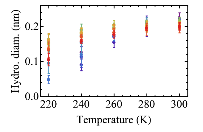
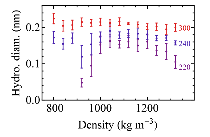
The normalization process used above removes the information about the absolute value of . If was the diffusion coefficient of a macroscopic object obeying hydrodynamics in the Stokes regime, would be related to the hydrodynamic diameter by:
| (5) |
Figure 10 shows computed from the simulation data. At high temperature, is –, nearly independent of (or only slightly decreasing with) density. To assess the validity of Eq. 5, should be compared to a molecular diameter determined independently. Several choices of this molecular diameter are possible (see for instance Ref. Cappelezzo et al., 2007 for a discussion in the case of the Lennard-Jones fluid). The volume per molecule in the liquid is around at , equivalent to a sphere of diameter , or if one considers random close-packed spheres occupying 64% of space. The Lennard-Jones parameter for interaction between the oxygen sites of two molecules in TIP4P/2005 is . Abascal and Vega (2005) All these values are close to . For a spherical object, a hydrodynamic diameter smaller than the physical diameter can be due to the slip boundary condition between the object and the ambient fluid Zwanzig and Bixon (1970). This can vary the factor in the denominator of Eq. 5 from (no slip) to (perfect slip). Slip could thus explain the values of for water at high temperature Sposito (1981). A change in slip boundary conditions may also explain changes in up to 50%, but cannot account for the large decrease at low temperature, which can exceed a factor of 10. An explanation based on slippage only should thus be discarded.
The behavior of water is reminiscent of many glassformers near their glass transition temperature . In this case, the decoupling between and is due to the emergence of dynamic heterogeneities, that is, transient, spatially correlated regions of particles with high and low mobility Tarjus and Kivelson (1995); Ediger and Harrowell (2012). Emergence of these regions at low temperature gives rise to a distribution of relaxation times broader than at high temperature. Because the different dynamic quantities result from different moments of the distribution, they start decoupling upon cooling. The SE violation in water has also been related to dynamic heterogeneities Becker, Poole, and Starr (2006); Mazza et al. (2007); Kumar et al. (2007); Guillaud et al. (2017a); Galamba (2017); Kawasaki and Kim (2017) ; however, the discussion was based on simulations of rather than of , and in contrast to usual glassformers for which the most mobile molecules cause the breakdown of the SE relation, all scales of mobility were involved in water. Further studies are needed to better understand the origin of the SE violation in water and its relation with the Widom line.
IV Conclusion
By performing extensive simulations of dynamic properties for the TIP4P/2005 water model, we have been able to reproduce nearly quantitatively all features observed for viscosity and self-diffusion coefficent of real water at temperatures below ambient, including the supercooled region, and in a broad positive pressure range. Our simulations also go beyond the conditions which have been hitherto explored in experiments. At lower temperatures, the minimum in and the maximum in as a function of density or pressure are found to become even more pronounced. At negative pressure, a maximum in and a minimum in are observed. The dynamic extension of the thermodynamic two-state model available for TIP4P/2005 is able to accurately reproduce the simulation data. Inclusion of a pressure dependence in the activation energy of the low density state is necessary to fit the negative pressure data, pointing to a large activation volume for the dynamics of this state. The Stokes-Einstein relation is strongly violated as the system is cooled through the Widom line. Our study provides a unifying framework to interpret the thermodynamic and dynamic anomalies of water, and calls for experiments on the dynamics of water at negative pressure.
Acknowledgments
PM, ES and CV have been funded by grants FIS2013/43209-P, FIS2016-78117-P and FIS2016-78847-P of the MEC and the UCM/Santander 910570 and PR26/16-10B-2. PM acknowledges financial support from a FPI PhD fellowship. LJ acknowledges support from Institut Universitaire de France. This work was partially supported by CNRS (France) through a PICS program.
Appendix A Simulation data
Tables 3 and 4 give all the simulation results of this study with their uncertainty (one standard deviation). For viscosity (Table 3), the uncertainty is the standard deviation of the five independent Green-Kubo integrals of the auto-correlation function of traceless stress tensor elements Chen, Smit, and Bell (2009). For self-diffusion (Table 4), the uncertainty was less straighforward to obtain, and we proceeded as follows. At each temperature, for one every three densities, we used the block averaging method on one of the trajectories. The selected trajectory was cut into four pieces with equal duration. For each piece, the self-diffusion coefficient for the finite system, , was calculated from the slope of the mean squared displacement in the diffusive regime as explained in Section II.1. The uncertainty on was taken as the standard deviation of the four values thus obtained. Table 4 gives the self-diffusion coefficient for the infinite liquid, after correction for finite size effects using Eq. 1. The total uncertainty on the corrected was calculated by propagating the uncertainty on and . Because the procedure was computationally costly, we applied it at every temperature, but only for one every three densities. At each temperature, for each remaining density, we assumed that the relative uncertainty on was equal to the relative uncertainty on at the nearest density for which it was directly calculated with the above method. Hence, absolute uncertainties on at the remaining densities were only calculated indirectly.
We note that, in order to get a more accurate estimate of the uncertainties, more simulations would be needed. The quantity we use to assess the quality of the fits is quite sensitive to the uncertainty, because it involves dividing by the squared uncertainties. Therefore the absolute values for could be modified if the uncertainty calculations were refined. Nevertheless, because fitting with the original or the modified two-state model uses the same definitions for the uncertainties, the comparison between the two fits is justified. Our results show that the modified model gives a better fit than the original one, and over a broader pressure range.
| Temperature () | |||||
|---|---|---|---|---|---|
| Density () | 220 | 240 | 260 | 280 | 300 |
| 800.43 | 37.5 (3.8) | 5.72 (0.45) | 1.73 (0.12) | 0.811 (0.046) | |
| 839.99 | 101 (17) | 8.46 (0.61) | 2.12 (0.30) | 0.961 (0.062) | |
| 879.49 | 82 (17) | 8.26 (0.59) | 2.157 (0.077) | 1.011 (0.062) | |
| 920.05 | 1348 (281) | 45.3 (9.0) | 5.58 (0.43) | 1.929 (0.089) | 0.926 (0.045) |
| 960.09 | 164 (46) | 15.9 (1.5) | 3.82 (0.25) | 1.57 (0.11) | 0.864 (0.032) |
| 999.26 | 36.8 (5.7) | 7.94 (0.56) | 2.753 (0.091) | 1.320 (0.037) | 0.834 (0.036) |
| 1040.59 | 20.3 (2.0) | 5.40 (0.41) | 2.20 (0.10) | 1.214 (0.014) | 0.808 (0.028) |
| 1080.66 | 15.5 (0.9) | 4.64 (0.13) | 2.114 (0.097) | 1.215 (0.056) | 0.816 (0.033) |
| 1119.05 | 13.8 (1.3) | 4.24 (0.15) | 2.04 (0.12) | 1.228 (0.028) | 0.8368 (0.0092) |
| 1159.29 | 14.4 (1.4) | 4.40 (0.24) | 2.15 (0.11) | 1.327 (0.084) | 0.933 (0.030) |
| 1199.42 | 14.8 (1.6) | 4.83 (0.28) | 2.44 (0.09) | 1.480 (0.093) | 1.029 (0.037) |
| 1239.28 | 22.6 (1.7) | 6.23 (0.18) | 2.84 (0.11) | 1.71 (0.12) | 1.189 (0.055) |
| 1280.93 | 33.7 (5.0) | 8.21 (0.23) | 3.54 (0.15) | 2.11 (0.19) | 1.48 (0.10) |
| 1319.79 | 78.2 (12) | 12.81 (0.24) | 5.02 (0.12) | 2.61 (0.10) | 1.770 (0.087) |
| Temperature () | |||||
| Density () | 220 | 240 | 260 | 280 | 300 |
| 800.43 | 0.0746 (0.0058) | 0.387 (0.022) | 1.152 (0.031) | 2.413 (0.072) | |
| 839.99 | 0.0386 (0.0030) | 0.291 (0.017) | 0.963 (0.026) | 2.235 (0.067) | |
| 879.49 | 0.0378 (0.0063) | 0.270 (0.011) | 0.949 (0.021) | 2.103 (0.046) | |
| 920.05 | 0.00497 (0.00067) | 0.065 (0.011) | 0.390 (0.016) | 1.089 (0.024) | 2.209 (0.048) |
| 960.09 | 0.0207 (0.0028) | 0.144 (0.024) | 0.517 (0.021) | 1.246 (0.028) | 2.392 (0.052) |
| 999.26 | 0.0576 (0.0020) | 0.255 (0.010) | 0.701 (0.032) | 1.450 (0.021) | 2.450 (0.061) |
| 1040.59 | 0.0976 (0.0033) | 0.342 (0.014) | 0.846 (0.039) | 1.579 (0.023) | 2.563 (0.064) |
| 1080.66 | 0.1353 (0.0046) | 0.423 (0.017) | 0.914 (0.042) | 1.666 (0.025) | 2.492 (0.062) |
| 1119.05 | 0.1455 (0.0060) | 0.453 (0.022) | 0.915 (0.033) | 1.627 (0.056) | 2.485 (0.029) |
| 1159.29 | 0.1490 (0.0061) | 0.437 (0.021) | 0.872 (0.032) | 1.519 (0.053) | 2.264 (0.026) |
| 1199.43 | 0.1353 (0.0056) | 0.402 (0.019) | 0.808 (0.029) | 1.387 (0.048) | 2.108 (0.024) |
| 1239.28 | 0.1044 (0.0073) | 0.331 (0.010) | 0.695 (0.037) | 1.224 (0.020) | 1.828 (0.033) |
| 1280.93 | 0.0715 (0.0050) | 0.2504 (0.0076) | 0.589 (0.031) | 1.019 (0.017) | 1.522 (0.027) |
| 1319.79 | 0.0392 (0.0027) | 0.1742 (0.0053) | 0.429 (0.023) | 0.803 (0.013) | 1.242 (0.022) |
Appendix B Arrhenius plots
Figure 11 gives a log-lin plot of and vs. inverse temperature.
References
- Gallo et al. (2016) P. Gallo, K. Amann-Winkel, C. A. Angell, M. A. Anisimov, F. Caupin, C. Chakravarty, E. Lascaris, T. Loerting, A. Z. Panagiotopoulos, J. Russo, J. A. Sellberg, H. E. Stanley, H. Tanaka, C. Vega, L. Xu, and L. G. M. Pettersson, Chem. Rev. 116, 7463 (2016).
- Debenedetti (2003) P. G. Debenedetti, Journal of Physics: Condensed Matter 15, R1669 (2003).
- Holten et al. (2012) V. Holten, C. E. Bertrand, M. A. Anisimov, and J. V. Sengers, The Journal of Chemical Physics 136, 094507 (2012).
- Röntgen (1884) W. C. Röntgen, Ann. Phys. 258, 510 (1884).
- Warburg and Sachs (1884) E. Warburg and J. Sachs, Ann. Phys. 258, 518 (1884).
- Bridgman (1925) P. W. Bridgman, Proceedings of the national academy of sciences 11, 603 (1925).
- Bett and Cappi (1965) K. E. Bett and J. B. Cappi, Nature 207, 620 (1965).
- Singh, Issenmann, and Caupin (2017) L. P. Singh, B. Issenmann, and F. Caupin, Proceedings of the National Academy of Sciences 114, 4312 (2017).
- Prielmeier et al. (1988) F. X. Prielmeier, E. W. Lang, R. J. Speedy, and H.-D. Lüdemann, Berichte der Bunsengesellschaft für physikalische Chemie 92, 1111 (1988).
- Harris and Newitt (1997) K. R. Harris and P. J. Newitt, Journal of Chemical & Engineering Data 42, 346 (1997).
- Lang and Lüdemann (1981) E. W. Lang and H. D. Lüdemann, Berichte der Bunsengesellschaft für physikalische Chemie 85, 603 (1981).
- Arnold and Lüdemann (2002) M. R. Arnold and H.-D. Lüdemann, Physical Chemistry Chemical Physics 4, 1581 (2002).
- Caupin (2015) F. Caupin, Journal of Non-Crystalline Solids 7th IDMRCS: Relaxation in Complex Systems, 407, 441 (2015).
- Holten et al. (2017) V. Holten, C. Qiu, E. Guillerm, M. Wilke, J. Rička, M. Frenz, and F. Caupin, The Journal of Physical Chemistry Letters 8, 5519 (2017).
- Poole et al. (1992) P. H. Poole, F. Sciortino, U. Essmann, and H. E. Stanley, Nature 360, 324 (1992).
- Poole, Saika-Voivod, and Sciortino (2005) P. H. Poole, I. Saika-Voivod, and F. Sciortino, Journal of Physics: Condensed Matter 17, L431 (2005).
- Agarwal, Alam, and Chakravarty (2011) M. Agarwal, M. P. Alam, and C. Chakravarty, The Journal of Physical Chemistry B 115, 6935 (2011).
- González et al. (2016) M. A. González, C. Valeriani, F. Caupin, and J. L. F. Abascal, The Journal of Chemical Physics 145, 054505 (2016).
- Biddle et al. (2017) J. W. Biddle, R. S. Singh, E. M. Sparano, F. Ricci, M. A. González, C. Valeriani, J. L. F. Abascal, P. G. Debenedetti, M. A. Anisimov, and F. Caupin, The Journal of Chemical Physics 146, 034502 (2017).
- Sciortino, Geiger, and Stanley (1991) F. Sciortino, A. Geiger, and H. E. Stanley, Nature 354, 218 (1991).
- Vaisman, Perera, and Berkowitz (1993) I. I. Vaisman, L. Perera, and M. L. Berkowitz, The Journal of Chemical Physics 98, 9859 (1993).
- Starr, Sciortino, and Stanley (1999) F. W. Starr, F. Sciortino, and H. E. Stanley, Phys. Rev. E 60, 6757 (1999).
- Scala et al. (2000) A. Scala, F. W. Starr, E. La Nave, F. Sciortino, and H. E. Stanley, Nature 406, 166 (2000).
- Errington and Debenedetti (2001) J. R. Errington and P. G. Debenedetti, Nature 409, 318 (2001).
- Ruocco et al. (1993) G. Ruocco, M. Sampoli, A. Torcini, and R. Vallauri, The Journal of Chemical Physics 99, 8095 (1993).
- Netz et al. (2001) P. A. Netz, F. W. Starr, H. E. Stanley, and M. C. Barbosa, The Journal of Chemical Physics 115, 344 (2001).
- Yeh and Hummer (2004) I.-C. Yeh and G. Hummer, J. Phys. Chem. B 108, 15873 (2004).
- Tazi et al. (2012) S. Tazi, A. Boţan, M. Salanne, V. Marry, P. Turq, and B. Rotenberg, J. Phys.: Condens. Matter 24, 284117 (2012).
- Shi, Debenedetti, and Stillinger (2013) Z. Shi, P. G. Debenedetti, and F. H. Stillinger, The Journal of Chemical Physics 138, 12A526 (2013).
- Guillaud et al. (2017a) E. Guillaud, S. Merabia, D. de Ligny, and L. Joly, Physical Chemistry Chemical Physics 19, 2124 (2017a).
- Guillaud et al. (2017b) E. Guillaud, L. Joly, D. de Ligny, and S. Merabia, The Journal of Chemical Physics 147, 014504 (2017b).
- González and Abascal (2010) M. A. González and J. L. F. Abascal, The Journal of Chemical Physics 132, 096101 (2010).
- Kiss and Baranyai (2014) P. T. Kiss and A. Baranyai, The Journal of Chemical Physics 140, 154505 (2014).
- Guevara-Carrion, Vrabec, and Hasse (2011) G. Guevara-Carrion, J. Vrabec, and H. Hasse, The Journal of Chemical Physics 134, 074508 (2011).
- Kawasaki and Kim (2017) T. Kawasaki and K. Kim, Science Advances 3, e1700399 (2017).
- Dhabal et al. (2016) D. Dhabal, C. Chakravarty, V. Molinero, and H. K. Kashyap, The Journal of Chemical Physics 145, 214502 (2016).
- Ma, Li, and Wang (2015) Z. Ma, J. Li, and F. Wang, The Journal of Physical Chemistry Letters 6, 3170 (2015).
- Vedamuthu, Singh, and Robinson (1994) M. Vedamuthu, S. Singh, and G. W. Robinson, The Journal of Physical Chemistry 98, 2222 (1994).
- Cho, Urquidi, and Robinson (1999) C. H. Cho, J. Urquidi, and G. W. Robinson, The Journal of Chemical Physics 111, 10171 (1999).
- Cho et al. (2002) C. H. Cho, J. Urquidi, S. Singh, S. C. Park, and G. W. Robinson, The Journal of Physical Chemistry A 106, 7557 (2002).
- Tanaka (2000) H. Tanaka, The Journal of Chemical Physics 112, 799 (2000).
- Tanaka (2003) H. Tanaka, Journal of Physics: Condensed Matter 15, L703 (2003).
- Holten, Sengers, and Anisimov (2014) V. Holten, J. V. Sengers, and M. A. Anisimov, Journal of Physical and Chemical Reference Data 43, 043101 (2014).
- Chang and Sillescu (1997) I. Chang and H. Sillescu, The Journal of Physical Chemistry B 101, 8794 (1997).
- Dehaoui, Issenmann, and Caupin (2015) A. Dehaoui, B. Issenmann, and F. Caupin, Proceedings of the National Academy of Sciences 112, 12020 (2015).
- Galamba (2017) N. Galamba, Journal of Physics: Condensed Matter 29, 015101 (2017).
- Abascal and Vega (2005) J. L. F. Abascal and C. Vega, The Journal of Chemical Physics 123, 234505 (2005).
- Plimpton (1995) S. Plimpton, Journal of Computational Physics 117, 1 (1995).
- Hockney and Eastwood (1988) R. Hockney and J. Eastwood, “Computer Simulation Using Particles,” https://www.crcpress.com/Computer-Simulation-Using-Particles/Hockney-Eastwood/p/book/9780852743928 (1988).
- Ryckaert, Ciccotti, and Berendsen (1977) J.-P. Ryckaert, G. Ciccotti, and H. J. C. Berendsen, Journal of Computational Physics 23, 327 (1977).
- Chen, Smit, and Bell (2009) T. Chen, B. Smit, and A. T. Bell, The Journal of Chemical Physics 131, 246101 (2009).
- Ramírez et al. (2010) J. Ramírez, S. K. Sukumaran, B. Vorselaars, and A. E. Likhtman, The Journal of Chemical Physics 133, 154103 (2010).
- Allen and Tildesley (2017) M. P. Allen and D. J. Tildesley, Computer Simulation of Liquids, new edition, second edition ed. (Oxford University Press, Oxford, New York, 2017).
- {The International Association for the Properties of Water and Steam} (2015) {The International Association for the Properties of Water and Steam}, “Guideline on Thermodynamic Properties of Supercooled Water,” Tech. Rep. IAPWS G12-15 ({The International Association for the Properties of Water and Steam}, 2015).
- Note (1) The value of for is chosen for consistency with the Stokes-Einstein-Debye relation , which holds at high temperature, similar to the Stokes-Einstein relation Dehaoui, Issenmann, and Caupin (2015).
- Abascal and Vega (2010) J. L. F. Abascal and C. Vega, The Journal of Chemical Physics 133, 234502 (2010).
- Sumi and Sekino (2013) T. Sumi and H. Sekino, RSC Advances 3, 12743 (2013).
- Yagasaki, Matsumoto, and Tanaka (2014) T. Yagasaki, M. Matsumoto, and H. Tanaka, Physical Review E 89 (2014), 10.1103/PhysRevE.89.020301.
- Singh et al. (2016) R. S. Singh, J. W. Biddle, P. G. Debenedetti, and M. A. Anisimov, The Journal of Chemical Physics 144, 144504 (2016).
- Overduin and Patey (2015) S. D. Overduin and G. N. Patey, The Journal of Chemical Physics 143, 094504 (2015).
- Handle and Sciortino (2018) P. H. Handle and F. Sciortino, The Journal of Chemical Physics 148, 134505 (2018).
- Wagner et al. (2011) W. Wagner, T. Riethmann, R. Feistel, and A. H. Harvey, Journal of Physical and Chemical Reference Data 40, 043103 (2011).
- Adam and Gibbs (1965) G. Adam and J. H. Gibbs, The Journal of Chemical Physics 43, 139 (1965).
- Gotze (1998) W. Gotze, Condensed Matter Physics 1, 873 (1998).
- Loerting et al. (2015) T. Loerting, V. Fuentes-Landete, P. H. Handle, M. Seidl, K. Amann-Winkel, C. Gainaru, and R. Böhmer, Journal of Non-Crystalline Solids 407, 423 (2015).
- Shephard and Salzmann (2016) J. J. Shephard and C. G. Salzmann, The Journal of Physical Chemistry Letters 7, 2281 (2016).
- Poole et al. (2011) P. H. Poole, S. R. Becker, F. Sciortino, and F. W. Starr, J. Phys. Chem. B 115, 14176 (2011).
- Nayar and Chakravarty (2013) D. Nayar and C. Chakravarty, Physical Chemistry Chemical Physics 15, 14162 (2013).
- Kumar et al. (2007) P. Kumar, S. V. Buldyrev, S. R. Becker, P. H. Poole, F. W. Starr, and H. E. Stanley, Proc. Natl. Acad. Sci. U.S.A. 104, 9575 (2007).
- Cappelezzo et al. (2007) M. Cappelezzo, C. A. Capellari, S. H. Pezzin, and L. A. F. Coelho, The Journal of Chemical Physics 126, 224516 (2007).
- Zwanzig and Bixon (1970) R. Zwanzig and M. Bixon, Physical Review A 2, 2005 (1970).
- Sposito (1981) G. Sposito, The Journal of Chemical Physics 74, 6943 (1981).
- Tarjus and Kivelson (1995) G. Tarjus and D. Kivelson, The Journal of Chemical Physics 103, 3071 (1995).
- Ediger and Harrowell (2012) M. D. Ediger and P. Harrowell, The Journal of Chemical Physics 137, 080901 (2012).
- Becker, Poole, and Starr (2006) S. Becker, P. Poole, and F. Starr, Physical Review Letters 97, 055901 (2006).
- Mazza et al. (2007) M. Mazza, N. Giovambattista, H. Stanley, and F. Starr, Physical Review E 76, 031203 (2007).