Who Learns Better Bayesian Network Structures: Accuracy and Speed of Structure Learning Algorithms

Abstract

Three classes of algorithms to learn the structure of Bayesian networks from data are common in the literature: constraint-based algorithms, which use conditional independence tests to learn the dependence structure of the data; score-based algorithms, which use goodness-of-fit scores as objective functions to maximise; and hybrid algorithms that combine both approaches. Constraint-based and score-based algorithms have been shown to learn the same structures when conditional independence and goodness of fit are both assessed using entropy and the topological ordering of the network is known [1].

In this paper, we investigate how these three classes of algorithms perform outside the assumptions above in terms of speed and accuracy of network reconstruction for both discrete and Gaussian Bayesian networks. We approach this question by recognising that structure learning is defined by the combination of a statistical criterion and an algorithm that determines how the criterion is applied to the data. Removing the confounding effect of different choices for the statistical criterion, we find using both simulated and real-world complex data that constraint-based algorithms are often less accurate than score-based algorithms, but are seldom faster (even at large sample sizes); and that hybrid algorithms are neither faster nor more accurate than constraint-based algorithms. This suggests that commonly held beliefs on structure learning in the literature are strongly influenced by the choice of particular statistical criteria rather than just by the properties of the algorithms themselves.

1 Background and Notation

Bayesian networks [BNs; 2] are a class of graphical models defined over a set of random variables $\mathbf{X}=\{X_{1},\ldots,X_{N}\}$, each describing some quantity of interest, that are associated with the nodes of a directed acyclic graph (DAG) $\mathcal{G}$. (They are often referred to interchangeably.) The structure of the DAG, that is, the set of arcs $A$ of $\mathcal{G}$, encodes the independence relationships between those variables, with graphical separation in $\mathcal{G}$ implying conditional independence in probability. As a result, $\mathcal{G}$ induces the factorisation

$$\operatorname{P}(\mathbf{X}\operatorname{|}\mathcal{G},\Theta)=\prod_{i=1}^{N}\operatorname{P}(X_{i}\operatorname{|}\Pi_{X_{i}},\Theta_{X_{i}}),$$ (1)

in which the global distribution of $\mathbf{X}$ (with parameters $\Theta$) decomposes in one local distribution for each $X_{i}$ (with parameters $\Theta_{X_{i}}$) conditional on its parents $\Pi_{X_{i}}$. This decomposition holds only in the absence of missing data, which we will assume in the following.

The DAG $\mathcal{G}$ does not uniquely identify a single BN: all BNs with the same underlying undirected graph and v-structures (patterns of arcs like $X_{i}\rightarrow X_{j}\leftarrow X_{k}$, with no arc between $X_{i}$ and $X_{k}$) fall into the same equivalence class [3] of models and are probabilistically indistinguishable. It is easy to see that the two other possible patterns of two arcs and three nodes result in equivalent factorisations:

$$\underbrace{\operatorname{P}(X_{i})\operatorname{P}(X_{j}\operatorname{|}X_{i})\operatorname{P}(X_{k}\operatorname{|}X_{j})}_{X_{i}\rightarrow X_{j}\rightarrow X_{k}}=\operatorname{P}(X_{j},X_{i})\operatorname{P}(X_{k}\operatorname{|}X_{j})=\underbrace{\operatorname{P}(X_{i}\operatorname{|}X_{j})\operatorname{P}(X_{j})\operatorname{P}(X_{k}\operatorname{|}X_{j})}_{X_{i}\leftarrow X_{j}\rightarrow X_{k}}.$$ (2)

Hence each equivalence class is represented by the completed partially-directed acyclic graph (CPDAG) that arises from the combination of these two quantities.

While in principle there are many possible choices for the distribution of $\mathbf{X}$, the literature has focused for the most part on two sets of assumptions:

• Discrete BNs [4] assume that the $X_{i}$ are multinomial random variables:

  $$X_{i}\operatorname{|}\Pi_{X_{i}}\sim\mathit{Mul}(\pi_{ik\operatorname{|}j}),\qquad\pi_{ik\operatorname{|}j}=\operatorname{P}(X_{i}=k\operatorname{|}\Pi_{X_{i}}=j);$$

  the $\pi_{ik\operatorname{|}j}$ are the conditional probabilities of $X_{i}$ given the $j$th configuration of the values of its parents. As a result, $\mathbf{X}$ is also multinomial. When learning BNs from data, generally we further assume positivity ($\pi_{ik\operatorname{|}j}>0$), parameter independence ($\pi_{ik\operatorname{|}j}$ for different parent configurations are independent) and parameter modularity ($\pi_{ik\operatorname{|}j}$ associated with different nodes are independent).

• Gaussian BNs [GBNs; 5] assume that the $X_{i}$ are univariate normal random variables linked by linear dependencies to their parents,

  $$X_{i}\operatorname{|}\Pi_{X_{i}}\sim N(\mu_{X_{i}}+\Pi_{X_{i}}\boldsymbol{\beta}_{X_{i}},\sigma^{2}_{X_{i}}),$$

  in what is essentially a linear regression model of $X_{i}$ against the $\Pi_{X_{i}}$ with regression coefficients $\boldsymbol{\beta}_{X_{i}}=\{\beta_{X_{i},X_{j}},X_{j}\in\Pi_{X_{i}}\}$. $\mathbf{X}$ is then multivariate normal, and we generally assume that its covariance matrix $\Sigma$ is positive definite. Equivalently [6], we can consider the precision matrix $\Omega=\Sigma^{-1}$ and parameterise the $X_{i}\operatorname{|}\Pi_{X_{i}}$ with the partial correlations

  $$\rho_{X_{i},X_{j}\operatorname{|}\Pi_{X_{i}}\setminus X_{j}}=\frac{\Omega_{ij}}{\sqrt{\Omega_{ii}\Omega_{jj}}}$$

  between $X_{i}$ and each parent $X_{j}\in\Pi_{X_{i}}$ given the rest, since

  $$\beta_{X_{i},X_{j}}=\rho_{X_{i},X_{j}\operatorname{|}\Pi_{X_{i}}\setminus X_{j}}\sqrt{\frac{\Omega_{ii}}{\Omega_{jj}}}.$$

Other distributional assumptions have seen less widespread adoption for various reasons. For instance, copulas [7] and truncated exponentials [8] lack exact conditional inference and simple closed-form estimators; and conditional linear Gaussian BNs [9] cannot encode DAGs with arcs pointing from discrete to continuous nodes.

2 Learning a Bayesian Network from Data

The task of learning a BN with DAG $\mathcal{G}$ and parameters $\Theta$ from a data set $\mathcal{D}$ containing $n$ observations can be performed in two steps in an inherently Bayesian fashion:

$$\underbrace{\operatorname{P}(\mathcal{G},\Theta\operatorname{|}\mathcal{D})}_{\text{learning}}=\underbrace{\operatorname{P}(\mathcal{G}\operatorname{|}\mathcal{D})}_{\text{structure learning}}\cdot\underbrace{\operatorname{P}(\Theta\operatorname{|}\mathcal{G},\mathcal{D})}_{\text{parameter learning}}.$$ (3)

Structure learning consists in finding the DAG $\mathcal{G}$ that encodes the dependence structure of the data; parameter learning consists in estimating the parameters $\Theta$ given the $\mathcal{G}$ obtained from structure learning. If we assume parameters in different local distributions are independent, they can be learned separately and efficiently for each node because (1) then implies

$$\operatorname{P}(\Theta\operatorname{|}\mathcal{G},\mathcal{D})=\prod_{i=1}^{N}\operatorname{P}(\Theta_{X_{i}}\operatorname{|}\Pi_{X_{i}},\mathcal{D}).$$

On the other hand, structure learning is well known to be NP-complete [10], even when assuming the availability of an independence and inference oracle [11]; only some relaxations such as [12] are not NP-hard. Using Bayes theorem once more, we can formulate it as

$$\operatorname{P}(\mathcal{G}\operatorname{|}\mathcal{D})\propto\operatorname{P}(\mathcal{G})\operatorname{P}(\mathcal{D}\operatorname{|}\mathcal{G});$$

and following (1) we can decompose the marginal likelihood $\operatorname{P}(\mathcal{D}\operatorname{|}\mathcal{G})$ into one component for each local distribution

$$\operatorname{P}(\mathcal{D}\operatorname{|}\mathcal{G})=\int\operatorname{P}(\mathcal{D}\operatorname{|}\mathcal{G},\Theta)\operatorname{P}(\Theta\operatorname{|}\mathcal{G})\,d\Theta=\\ =\prod_{i=1}^{N}\int\operatorname{P}(X_{i}\operatorname{|}\Pi_{X_{i}},\Theta_{X_{i}})\operatorname{P}(\Theta_{X_{i}}\operatorname{|}\Pi_{X_{i}})\,d\Theta_{X_{i}}.$$ (4)

Closed-form expressions for (4) are available for both discrete BNs and GBNs; and (4) can be approximated using the Bayesian information criterion (BIC) [13] as well. Both will be described in Section 2.2. As for $\operatorname{P}(\mathcal{G})$, the most common choice in the literature is the uniform distribution; we will default to it in the following as well. The space of the DAGs grows super-exponentially in $N$ [14] and that makes it cumbersome to specify informative priors: two notable exceptions are presented in [15] and [16]. [15] described a completed prior in which they elicitated prior probabilities for a subset of arcs and completed the prior to cover the remaining arcs with a discrete uniform distribution. As an alternative, [16] proposed an informative prior using a log-linear combination of arbitrary patterns of arcs. Some structure learning approaches [e.g. 17] also assume the topological ordering of $\mathcal{G}$ to be known a priori and assign a prior probability of zero to any DAG that is incompatible with that ordering. This effectively assigns a prior probability of zero to many arcs; and it completely side-steps the identifiability issues arising from the existence of equivalence classes because, for each arc, only one direction is compatible with the topological ordering.

2.1 Structure Learning Algorithms

Several algorithms have been proposed to implement BN structure learning, following one of three possible approaches: constraint-based, score-based and hybrid.

Algorithm 1 PC-Stable Algorithm

Input: a data set $\mathcal{D}$ from $\mathbf{X}$, a (conditional) independence test $\mathit{Test}(X_{i},X_{j}\operatorname{|}\mathbf{S};\mathcal{D})$.
Output: a CPDAG $\mathcal{G}$.

1. Initialise a complete undirected graph $\mathcal{G}$ spanning $\mathbf{X}$.

2. For $l=0,1,\ldots,N-2$:

   1. For all adjacent pairs of nodes $(X_{i},X_{j}),i\neq j$ such that $X_{i}$ has at least $l$ neighbours in the current $\mathcal{G}$, excluding $X_{j}$:

      1. Choose a new subset $\mathbf{S}$ of size $l$ from the neighbours of $X_{i}$ excluding $X_{j}$;

      2. If $\mathit{Test}(X_{i},X_{j}\operatorname{|}\mathbf{S};\mathcal{D})$ accepts the hypothesis that $X_{i}$ is independent from $X_{j}$ given $\mathbf{S}$, remove $X_{i}-X_{j}$ from $\mathcal{G}$ and set $\mathbf{S}_{X_{i}X_{j}}=\mathbf{S}$ as the separating set of ($X_{i},X_{j})$.

      3. If $X_{i}$ and $X_{j}$ are no longer adjacent or there are no more possible subsets $\mathbf{S}$ of size $l$ to consider, move to the next pair of nodes.

3. For each triplet $X_{i}-X_{k}-X_{j}$ such that $X_{i}$ is not adjacent to $X_{j}$ and that $X_{k}\notin\mathbf{S}_{X_{i}X_{j}}$, replace it with the v-structure $X_{i}\rightarrow X_{k}\leftarrow X_{j}$.

4. Set more arc directions by applying recursively the following two rules:

   1. if $X_{i}$ is adjacent to $X_{j}$ and there is a strictly directed path from $X_{i}$ to $X_{j}$ then replace $X_{i}-X_{j}$ with $X_{i}\rightarrow X_{j}$ (to avoid introducing cycles);

   2. if $X_{i}$ and $X_{j}$ are not adjacent but $X_{i}\rightarrow X_{k}$ and $X_{k}-X_{j}$, then replace the latter with $X_{k}\rightarrow X_{j}$ (to avoid introducing new v-structures).

Constraint-based algorithms are based on the seminal work of Pearl on causal graphical models [18], which found its first practical implementation in the PC algorithm [19]. Its modern implementation, called PC-stable [20], is illustrated in Algorithm 1. Steps 1 and 2 identify which pairs of variables $(X_{i},X_{j})$ are connected by an arc, regardless of its direction. Such variables cannot be separated by any subset of the other variables; this condition is tested heuristically by performing a sequence of conditional independence tests $\mathit{Test}(X_{i},X_{j}\operatorname{|}\mathbf{S};\mathcal{D})$ with increasingly large candidate separating sets $\mathbf{S}$. Step 3 identifies the v-structures among all the pairs of non-adjacent nodes $X_{i}$ and $X_{j}$ with a common neighbour $X_{k}$ using the separating sets found in step 2. At the end of step 3 both the skeleton and the v-structures of the network are known; step 4 then sets the remaining arc directions using the rules from [3] to obtain the CPDAG describing the identified equivalence class. More recent algorithms such as Grow-Shrink (GS) [21] and Inter-IAMB [22] proceed along similar lines, but use faster heuristics to implement the first two steps; an overview can be found in [23].

Algorithm 2 Greedy Search

Input: a data set $\mathcal{D}$ from $\mathbf{X}$, an initial (usually empty) DAG $\mathcal{G}$, a score function $\mathit{Score}(\mathcal{G},\mathcal{D})$.
Output: the DAG $\mathcal{G}_{\mathit{max}}$ that maximises $\mathit{Score}(\mathcal{G},\mathcal{D})$.

1. Compute the score of $\mathcal{G}$, $S_{\mathcal{G}}=\mathit{Score}(\mathcal{G},\mathcal{D})$, and set $S_{\mathit{max}}=S_{\mathcal{G}}$ and $\mathcal{G}_{\mathit{max}}=\mathcal{G}$.

2. Hill climbing: repeat as long as $S_{\mathit{max}}$ increases:

   1. for every possible arc addition, deletion or reversal in $\mathcal{G}_{\mathit{max}}$ resulting in a DAG:

      1. compute the score of the modified DAG $\mathcal{G}^{*}$, $S_{\mathcal{G}^{*}}=\mathit{Score}(\mathcal{G}^{*},\mathcal{D})$:

      2. if $S_{\mathcal{G}^{*}}>S_{\mathit{max}}$ and $S_{\mathcal{G}^{*}}>S_{\mathcal{G}}$, set $\mathcal{G}=\mathcal{G}^{*}$ and $S_{\mathcal{G}}=S_{\mathcal{G}^{*}}$.

   2. if $S_{\mathcal{G}}>S_{\mathit{max}}$, set $S_{\mathit{max}}=S_{\mathcal{G}}$ and $\mathcal{G}_{\mathit{max}}=\mathcal{G}$.

3. Tabu list: for up to $t_{0}$ times, repeat step 2 but choose the DAG $\mathcal{G}$ with the highest $S_{\mathcal{G}}$ that has not been visited in the last $t_{1}$ steps regardless of $S_{\mathit{max}}$. If a DAG such that $S_{\mathcal{G}}>S_{\mathit{max}}$ is found, restart the search from step 2.

4. Random restart: for up to $r$ times, perturb $\mathcal{G}_{\mathit{max}}$ with multiple arc additions, deletions and reversals to obtain a new DAG $\mathcal{G}^{\prime}$ and search from step 2.

Score-based algorithms represent the application of general-purpose optimisation techniques to BN structure learning. Each candidate DAG is assigned a network score reflecting its goodness of fit, which the algorithm then attempts to maximise. Some examples are heuristics such as greedy search, simulated annealing [24] and genetic algorithms [25]; a comprehensive review of these and other approaches is provided in [26]. They can also be applied to CPDAGs, as in the case of Greedy Equivalent Search [GES; 27]. In recent years exact maximisation of $\operatorname{P}(\mathcal{G}\operatorname{|}\mathcal{D})$ and BIC has become feasible as well for small data sets thanks to increasingly efficient pruning of the space of the DAGs and tight bounds on the scores [28, 29, 30]. Another possible choice is exploring the space of DAGs using Markov chain Monte Carlo methods, which have the advantage of producing a sample of DAGs from $\operatorname{P}(\mathcal{G}\operatorname{|}\mathcal{D})$ thus making posterior inference possible. This approach, which dates back to [31], has been improved upon [32, 33] by first sampling from the space of topological orderings to accelerate mixing.

Greedy search, illustrated in Algorithm 2, represents by far the most common group score-based algorithm in practical applications. It consists of an initialisation phase (step 1) followed by a hill climbing search (step 2), which is then optionally refined with a tabu list (step 3) and random restarts (step 4). In each iteration, hill climbing tries to delete and to reverse each arc in the current candidate DAG $\mathcal{G}_{\mathit{max}}$; and to add each possible arc that is not already present in $\mathcal{G}_{\mathit{max}}$ and that does not introduce any cycles. These are local moves that impact only one or two local distributions in th BN, which greatly reduces the computational complexity of greedy search by avoiding the need to re-score all nodes at each iterations. The resulting $\mathcal{G}$ with the highest score $S_{\mathcal{G}}$ is compared to $\mathcal{G}_{\mathit{max}}$; if it has a better score ($S_{\mathcal{G}}>S_{\mathit{max}}$) then $\mathcal{G}$ becomes the new $\mathcal{G}_{\mathit{max}}$. If, on the other hand, $S_{\mathcal{G}}<S_{\mathit{max}}$, greedy search has reached an optimum. There is no guarantee that $\mathcal{G}$ is a global optimum; hence greedy search may perform further steps to reduce the chances that $\mathcal{G}$ is in fact a sub-optimal local optimum. One option is to restart the search in step 2 from a different starting point, obtained by changing $r$ arcs in the current optimal $\mathcal{G}$. This gives what is called the hill climbing with random restarts algorithm. Another option is to keep a tabu list of previously-visited DAGs and to continue searching for a better DAG that has yet been considered, giving the tabu search algorithm. Clearly, it is possible to perform both steps 3 and 4 and obtain a tabu search with random restarts.

Algorithm 3 A Simulated Annealing Approach to Structure Learning

Input: a data set $\mathcal{D}$, and initial node ordering $\mathcal{T}_{0}$, a score function $\mathit{Score}(\mathcal{G},\mathcal{D})$
Output: the DAG $\mathcal{G}_{\mathit{max}}$ that maximises $\mathit{Score}(\mathcal{G},\mathcal{D})$.

1. For a large number of iterations i = 1, …, m:

   1. Generate a new topological ordering $\mathcal{T}_{i}$ by randomly permuting the nodes in $\mathcal{T}_{i-1}$.

   2. Accept the new ordering with some probability $\operatorname{P}(\mathcal{T}_{i}\operatorname{|}\mathcal{T}_{i-1},\beta)$, where $\beta$ is the temperature; otherwise $\mathcal{T}_{i}=\mathcal{T}_{i-1}$.

   3. Reduce the temperature $\beta$.

2. For the best ordering $\widehat{\mathcal{T}}$, find the $\mathcal{G}$ with the highest $\mathit{Score}(\mathcal{G},\mathcal{D}\operatorname{|}\widehat{\mathcal{T}})$.

A second group of score-based algorithms seek to speed-up structure learning by first obtaining a topological ordering $\mathcal{T}$ for the nodes, and then learning the optimal $\mathcal{G}\operatorname{|}\mathcal{T}$ for the optimal $\mathcal{T}$. The first approach of this kind was the K2 algorithm [17], which assumed $\mathcal{T}$ to be known a priori; other algorithms such as [34] and more recently [35] learn the variable ordering from the data. Among these algorithms, we will focus on the simulated annealing [36] modification of the Metropolis-Hastings topological ordering search covered in [2]. The algorithm is illustrated in Algorithm 3: step 1 maximises $\operatorname{P}(\mathcal{T}\operatorname{|}\mathcal{D})$, while step 2 maximises $\operatorname{P}(\mathcal{G}\operatorname{|}\mathcal{T},\mathcal{D})$. Hence Algorithm 3 maximises

$$\operatorname{P}(\mathcal{G}\operatorname{|}\mathcal{D})=\operatorname{P}(\mathcal{G},\mathcal{T}\operatorname{|}\mathcal{D})=\operatorname{P}(\mathcal{T}\operatorname{|}\mathcal{D})\operatorname{P}(\mathcal{G}\operatorname{|}\mathcal{T},\mathcal{D})$$

since the topological ordering $\mathcal{T}$ is a function of $\mathcal{G}$. Step 1 generates a new topological ordering $\mathcal{T}_{i}$ at each iteration, which then is carried forward to the next iteration with a transition probability $\operatorname{P}(\mathcal{T}_{i}\operatorname{|}\mathcal{T}_{i-1},\beta)$ that depends on the relative goodness-of-fit of of $\mathcal{T}_{i}$ and $\mathcal{T}_{i-1}$. The latter can be calculated either by averaging over all possible DAGs compatible with each topological ordering

$$\operatorname{P}(\mathcal{T}\operatorname{|}\mathcal{D})\propto\operatorname{P}(\mathcal{D}\operatorname{|}\mathcal{T})\propto\int\operatorname{P}(\mathcal{D}\operatorname{|}\mathcal{G})\operatorname{P}(\mathcal{G}\operatorname{|}\mathcal{T})\,d\mathcal{G};$$ (5)

or by finding the DAG with the best score for each topological ordering subject to some constraints such as the maximum number of parents for each node. The role of $\beta$ is to control the annealing schedule by gradually reducing the transition probability.

Finally, hybrid algorithms combine the previous two approaches. They consist of two steps, called restrict and maximise. In the first step, a candidate set $\mathbf{C}_{X_{i}}$ of parents is selected for each node $X_{i}$ from $\mathbf{X}\setminus X_{i}$ using conditional independence tests. Assuming that all $\mathbf{C}_{X_{i}}$ are small compared to $\mathbf{X}$, we are left with a smaller and more regular space in which to search for our network structure. The second step seeks the DAG that maximises a given network score function subject to the constraint that the parents of each $X_{i}$ must be in the corresponding $\mathbf{C}_{X_{i}}$. In practice, the first step is implemented using the part of some constraint-based algorithm that identified the skeleton of the network, corresponding to steps 1 and 2 in Algorithm 1. The second step, on the other hand, is implemented using a score-based algorithm such as Algorithms 2 and 3 above. The best-known member of this family is the Max-Min Hill Climbing algorithm (MMHC) by [37]; two other examples are RSMAX2 from our previous work [38] and H²PC [39].

2.2 Statistical Criteria: Conditional Independence Tests and Network Scores

The choice of which statistical criterion to use in structure learning, be that a conditional independence test or a network score, depends mainly on the distribution of $\mathbf{X}$; and is orthogonal to the choice of algorithm. Here we provide a brief overview of those in widespread use in the literature, while referring the reader to [2] for a more comprehensive treatment.

For discrete BNs, conditional independence tests are functions of the observed frequencies $\{n_{ijk};i=1,\ldots,R,$ $j=1,\ldots,C;k=1,\ldots,L\}$ for any pair of variables ($X$, $Y$) given the configurations of some conditioning variables $\mathbf{Z}$. In other words, $X$, $Y$ and $\mathbf{Z}$ take one of $R$, $C$ and $L$ possible values for each observation. The two most common tests are the log-likelihood ratio $\mathrm{G}^{2}$ test and Pearson’s $\mathrm{X}^{2}$ test. $\mathrm{G}^{2}$ is defined as

$$\mathrm{G}^{2}(X,Y\operatorname{|}\mathbf{Z})=2\log\frac{\operatorname{P}(X\operatorname{|}Y,\mathbf{Z})}{\log\operatorname{P}(X\operatorname{|}\mathbf{Z})}=2\sum_{i=1}^{R}\sum_{j=1}^{C}\sum_{k=1}^{L}n_{ijk}\log\frac{n_{ijk}n_{++k}}{n_{i+k}n_{+jk}},$$ (6)

where $n_{i+k}=\sum_{j=1}^{C}n_{ijk}$, $n_{+jk}=\sum_{i=1}^{R}n_{ijk}$ and $n_{++k}=\sum_{i=1}^{R}\sum_{j=1}^{C}n_{ijk}$ are the marginal counts for $i,k$ (summed over $i$); $j,k$ (summed over $i$); and $k$ (summed over $i$ and $j$). $\mathrm{X}^{2}$ is defined as

$$\mathrm{X}^{2}(X,Y\operatorname{|}\mathbf{Z})=\sum_{i=1}^{R}\sum_{j=1}^{C}\sum_{k=1}^{L}\frac{\left(n_{ijk}-m_{ijk}\right)^{2}}{m_{ijk}}, m_{ijk}=\frac{n_{i+k}n_{+jk}}{n_{++k}}.$$ where

Both are asymptotically equivalent and have the same $\chi^{2}_{(R-1)(C-1)L}$ null distribution. Notably, $\mathrm{G}^{2}$ is also numerically equivalent to mutual information (they differ by a $2n$ factor).

For GBNs, conditional independence tests are functions of the partial correlation coefficients $\rho_{XY\operatorname{|}\mathbf{Z}}$. The log-likelihood ratio (and Gaussian mutual information) test takes form

$$\mathrm{G}^{2}(X,Y\operatorname{|}\mathbf{Z})=n\log(1-\rho_{XY\operatorname{|}\mathbf{Z}}^{2})\sim\chi^{2}_{1}.$$ (7)

Other common options are the exact Student’s $t$ test

$$\mathrm{t}(X,Y\operatorname{|}\mathbf{Z})=\rho_{XY\operatorname{|}\mathbf{Z}}\sqrt{\frac{n-|\mathbf{Z}|-2}{1-\rho_{XY\operatorname{|}\mathbf{Z}}^{2}}}\sim t_{n-|\mathbf{Z}|-2};$$

and the asymptotic Fisher’s $Z$ test, defined as

$$\mathrm{Z}(X,Y\operatorname{|}\mathbf{Z})=\log\left(\frac{1+\rho_{XY\operatorname{|}\mathbf{Z}}}{1-\rho_{XY\operatorname{|}\mathbf{Z}}}\right)\frac{\sqrt{n-|\mathbf{Z}|-3}}{2}\sim N(0,1).$$

As for network scores, the Bayesian Information criterion

$$\mathrm{BIC}(\mathcal{G};\mathcal{D})=\sum_{i=1}^{N}\left[\;\log\operatorname{P}(X_{i}\operatorname{|}\Pi_{X_{i}})-\frac{|\Theta_{X_{i}}|}{2}\log n\;\right],$$ (8)

is a common choice for both discrete BNs and GBNs, because it provides a simple approximation to $\log\operatorname{P}(\mathcal{G}\operatorname{|}\mathcal{D})$ that does not depend on any hyperparameter. $\log\operatorname{P}(\mathcal{G}\operatorname{|}\mathcal{D})$ is also available in closed form for both discrete BNs and GBNs.

In discrete BNs, $\operatorname{P}(\mathcal{D}\operatorname{|}\mathcal{G})$ is called the Bayesian Dirichlet (BD) score [4] and it is constructed using a conjugate Dirichlet prior with imaginary sample size $\boldsymbol{\alpha}$ (the size of an imaginary sample supporting the prior distribution, giving the weight given to the prior compared to the data). It takes the form

$$\operatorname{BD}(\mathcal{G},\mathcal{D};\boldsymbol{\alpha})=\prod_{i=1}^{N}\operatorname{BD}(X_{i}\operatorname{|}\Pi_{X_{i}};\alpha_{i})=\prod_{i=1}^{N}\prod_{j=1}^{q_{i}}\left[\frac{\Gamma(\alpha_{ij})}{\Gamma(\alpha_{ij}+n_{ij})}\prod_{k=1}^{r_{i}}\frac{\Gamma(\alpha_{ijk}+n_{ijk})}{\Gamma(\alpha_{ijk})}\right]$$ (9)

where

• $r_{i}$ is the number of states of $X_{i}$;

• $q_{i}$ is the number of configurations of $\Pi_{X_{i}}$;

• $n_{ij}=\sum_{k}n_{ijk}$, the marginal count for the $k$th parents configuration;

• the $\alpha_{ijk}$ are the hyperparameters of the Dirichlet distribution, and $\alpha_{ij}=\sum_{k}\alpha_{ijk}$, $\alpha_{i}=\sum_{j}\alpha_{ij}$.

The most common choice for the hyperparameters is $\alpha_{ijk}=\alpha_{i}/(r_{i}q_{i})$, which gives the Bayesian Dirichlet equivalent uniform (BDeu) score, the only BD score that satisfies score equivalence. It is typically used with small imaginary sample sizes such as $\alpha_{i}=1$ as suggested by [2] and [41]. Alternative BD scores have been proposed in [42] and [43, 44].

As for GBNs, $\log\operatorname{P}(\mathcal{D}\operatorname{|}\mathcal{G})$ is called the Bayesian Gaussian equivalent (BGe) score and it is constructed using a conjugate normal-Wishart prior for $\mathbf{X}$ with expected values $\boldsymbol{\nu}$ (for the mean) and $T$ (for the covariance). It takes the form [45]

$$\operatorname{BG}(\mathcal{G},\mathcal{D};\alpha_{w},\alpha_{\mu},T,\boldsymbol{\nu}) =\prod_{i=1}^{N}\operatorname{BG}(X_{i}\operatorname{|}\Pi_{X_{i}};\alpha_{w},\alpha_{\mu},T,\boldsymbol{\nu})$$

$$=\prod_{i=1}^{N}\prod_{j=1}^{q_{i}}\left(\frac{\alpha_{\mu}}{n+\alpha_{\mu}}\right)\frac{\Gamma\left(\frac{n+\alpha_{w}-N+|\Pi_{X_{i}}|+1}{2}\right)}{\pi^{n/2}\Gamma\left(\frac{\alpha_{w}-N+|\Pi_{X_{i}}|+1}{2}\right)}$$

$$\qquad\cdot\frac{\left|T_{X_{i},\Pi_{X_{i}}}\right|^{\frac{\alpha_{w}-N-|\Pi_{X_{i}}|-1}{2}}}{\left|T_{\Pi_{X_{i}}}\right|^{\frac{\alpha_{w}-N-|\Pi_{X_{i}}|}{2}}}\frac{\left|R_{\Pi_{X_{i}}}\right|^{\frac{n+\alpha_{w}-N-|\Pi_{X_{i}}|}{2}}}{\left|R_{X_{i},\Pi_{X_{i}}}\right|^{\frac{n+\alpha_{w}-N-|\Pi_{X_{i}}|-1}{2}}}$$ (10)

where:

• $\alpha_{\mu}$ and $\alpha_{w}$ are the imaginary sample sizes that give the weight of the normal and Wishart components of the prior compared to the sample;

• $R$ is the posterior covariance matrix and is given by

  $$R=T+S_{n}+\frac{n\alpha_{\mu}}{n+\alpha_{\mu}}(\overline{\mathbf{x}}-\boldsymbol{\nu})^{T}(\overline{\mathbf{x}}-\boldsymbol{\nu}), \bar{\mathbf{x}}=\frac{1}{n}\sum_{i=1}^{n}\mathbf{x}_{i},\quad S_{n}=\sum_{i=1}^{n}(\mathbf{x}_{i}-\overline{\mathbf{x}})(\mathbf{x}_{i}-\overline{\mathbf{x}})^{T},$$

  where $\mathbf{x}_{i}$ is a complete instantiation of $\mathbf{X}$;

• $T_{X_{i},\Pi_{X_{i}}}$ and $R_{X_{i},\Pi_{X_{i}}}$ are the submatrices of $T$ and $R$ corresponding to the ($X_{i}$, $\Pi_{X_{i}}$);

• similarly, $T_{\Pi_{X_{i}}}$ and $R_{\Pi_{X_{i}}}$ are the submatrices of $T$ and $R$ corresponding to the $\Pi_{X_{i}}$.

[45] suggests using the smallest valid values for both imaginary sample sizes ($\alpha_{\mu}=1$, $\alpha_{w}=N+2$), a diagonal $T=tI_{N}$ with

$$t=\frac{\alpha_{\mu}(\alpha_{w}-N-1)}{\alpha_{\mu}+1},$$

and $\boldsymbol{\nu}=\overline{\mathbf{x}}$ as a set of default values with wide applicability for the hyperparameters.

3 Performance as a Combination of Statistical Criteria and Algorithms

As it may be apparent from Sections 2.1 and 2.2, we take the view that the algorithms and the statistical criteria they use are separate and complementary in determining the overall behaviour of structure learning. Cowell [1] followed the same reasoning when showing that constraint-based and score-based algorithms can select identical discrete BNs. He noticed that the $\mathrm{G}^{2}$ test in (6) has the same expression as a score-based network comparison based on the log-likelihoods $\log\operatorname{P}(X\operatorname{|}Y,\mathbf{Z})-\log\operatorname{P}(X\operatorname{|}\mathbf{Z})$ if we take $\mathbf{Z}=\Pi_{X}$. He then showed that these two classes of algorithms are equivalent if we assume a fixed, known topological ordering and we use log-likelihood and $\mathrm{G}^{2}$ as matching statistical criteria.

In this paper we will complement that investigation by addressing the following questions:

1. Which of constraint-based and score-based algorithms provide the most accurate structural reconstruction, after accounting for the effect of the choice of statistical criteria?

2. Are constraint-based algorithms faster than score-based algorithms, or vice-versa?

3. Are hybrid algorithms more accurate than constraint-based or score-based algorithms?

4. Are hybrid algorithms faster than constraint-based or score-based algorithms?

5. Do the different classes of algorithms present any systematic difference in either speed or accuracy when learning small networks and large networks?

More precisely, we will drop the assumption that the topological ordering is known and we will compare the performance of different classes of algorithms outside of their equivalence conditions for both discrete BNs and GBNs. We choose questions Q1, Q2, Q3, Q4 and Q5 because they are most common among practitioners [e.g. 46] and researchers [e.g. 37, 2, 47]. Overall, there is a general view in these references and in the literature that score-based algorithms are less sensitive to individual errors of the statistical criteria, and thus more accurate, because they can reverse earlier decisions; and that hybrid algorithms are faster and more accurate than both score-based and constraint-based algorithms. These differences have been found to be more pronounced at small sample sizes. Furthermore, score-based algorithms have been found to scale less well to high-dimensional data.

We find two important limitations in such investigations. The first is that they focus almost exclusively on discrete BNs, ignoring that GBNs are based on very different distributional assumptions and thus that their conclusions will not necessarily hold for the latter. The second is the confounding between the choice of the algorithms and that of the statistical criteria, which makes it impossible to assess the merits inherently attributable to the algorithms themselves. Therefore, similarly to [1], we construct matching statistical criteria in the form of pairs of scores and independence tests that make algorithms directly comparable. Without loss of generality, consider two DAGs $\mathcal{G}^{+}$ and $\mathcal{G}^{-}$ which differ by a single arc $X_{j}\rightarrow X_{i}$. In a score-based approach, we can compare them using BIC from (8) and select $\mathcal{G}^{+}$ over $\mathcal{G}^{-}$ if

$$\mathrm{BIC}(\mathcal{G}^{+};\mathcal{D})>\mathrm{BIC}(\mathcal{G}^{-};D)\Rightarrow 2\log\frac{\operatorname{P}(X_{i}\operatorname{|}\Pi_{X_{i}}\cup\{X_{j}\})}{\operatorname{P}(X_{i}\operatorname{|}\Pi_{X_{i}})}>(|\Theta_{X_{i}}^{\mathcal{G}^{+}}|-|\Theta_{X_{i}}^{\mathcal{G}^{-}}|)\log n$$ (11)

which is equivalent to testing the conditional independence of $X_{i}$ and $X_{j}$ given $\Pi_{X_{i}}$ using the $\mathrm{G}^{2}$ test from (6) or (7), just with a different significance threshold than a $\chi^{2}_{1-\alpha}$ quantile at a pre-determined significance level $\alpha$. We will call this test $\mathrm{G}^{2}_{\mathrm{BIC}}$ and use it as the matching statistical criterion for $\mathrm{BIC}$ to compare different learning algorithms. In addition, we will construct a second test along the same lines using graph posterior probabilities in order to confirm our conclusions with a second set of matching criteria. Following (11), we write

$$\log\operatorname{P}(\mathcal{G}^{+}\operatorname{|}\mathcal{D})>\log\operatorname{P}(\mathcal{G}^{-}\operatorname{|}\mathcal{D})\Rightarrow\log\mathrm{BF}=\log\frac{\operatorname{P}(\mathcal{G}^{+}\operatorname{|}\mathcal{D})}{\operatorname{P}(\mathcal{G}^{-}\operatorname{|}\mathcal{D})}>0$$

which decides between $\mathcal{G}^{+}$ and $\mathcal{G}^{-}$ using a Bayes factor with a threshold of $1$, similarly to what was previously done in [48]. The resulting ($\mathrm{BIC}$, $\mathrm{G}^{2}_{\mathrm{BIC}}$) and ($\log\operatorname{P}(\mathcal{G}\operatorname{|}\mathcal{D})$, $\log\mathrm{BF}$) will be used to investigate discrete BNs and GBNs in the following section. An extension of ($\mathrm{BIC}$, $\mathrm{G}^{2}_{\mathrm{BIC}}$) to the family of matching criteria $(\mathrm{BIC}_{\gamma},\mathrm{G}^{2}_{\mathrm{BIC}_{\gamma}})$ will be used to investigate GBNs learned from real-world complex data in Section 5.

4 Simulation Study

We address Q1, Q2, Q3, Q4 and Q5 with a simulation study based on reference BNs from the Bayesian network repository [49]; we will later confirm our conclusions using real-world complex climate data in Section 5. Both will be implemented using the bnlearn [50] and catnet [36] R packages and TETRAD [51] via the r-causal R package [52].

We assess the structure learning algorithms listed in Table 2: three constraint-based (PC-Stable, GS, Inter-IAMB), three score-based (tabu search, simulated annealing for BIC, GES for $\log\operatorname{P}(\mathcal{G}\operatorname{|}\mathcal{D})$) and three hybrid algorithms (MMHC, RSMAX2, H²PC). For this purpose we use the 10 discrete BNs and 4 GBNs in Table 2. For each BN:

1. We generate $20$ samples of size $n/|\Theta|=0.1$, $0.2$, $0.5$, $1.0$, $2.0$, and $5.0$ to allow for meaningful comparisons between BNs of very different size and complexity. Intuitively, an absolute sample of size of, say, $n=1000$ may be large enough to learn reliably a small BN with few parameters, say $|\Theta|=100$, but it may be too small for a larger or denser network with $|\Theta|=10000$. Using the relative sample size $n/|\Theta|$ ensures small and large sample regimes are consistent for different BNs.

2. We learn $\mathcal{G}$ using (BIC, $\mathrm{G}^{2}_{\mathrm{BIC}}$) and ($\log\operatorname{P}(\mathcal{G}\operatorname{|}\mathcal{D})$, $\log\mathrm{BF}$). For the latter we use the BDeu and BGe scores in (9) and (10) with the hyperparameter values suggested in Section 2.2. In addition we set a prior probability of inclusion of $1/(N-1)$ for each parent of each node, which is the default in TETRAD.

3. We measure the accuracy of the learned DAGs using the Structural Hamming Distance [SHD; 37] from the reference BN scaled by the number of arcs $|A|$ of that BN (lower is better). This again motivated by the need to compare networks of different sizes: if both the reference BN and the learned network are sparse then we expect SHD to be $O(|A|)$, since both will have $O(|A|)$ arcs.

4. We measure the speed of the learning algorithms with the number of calls to the statistical criterion (lower is better). This is a classic measure of computational complexity in BN structure learning.

algorithm	class	discrete BNs	GBNs	(BIC, $\mathrm{G}^{2}_{\mathrm{BIC}}$)	($\log\operatorname{P}(\mathcal{G}\operatorname{|}\mathcal{D})$, $\log\mathrm{BF}$)
PC-Stable	constraint-based	$\checkmark$	$\checkmark$	$\checkmark$	$\checkmark$
Grow-Shrink (GS)	constraint-based	$\checkmark$	$\checkmark$	$\checkmark$	$\checkmark$
Inter-IAMB	constraint-based	$\checkmark$	$\checkmark$	$\checkmark$	$\checkmark$
tabu search	score-based	$\checkmark$	$\checkmark$	$\checkmark$	$\checkmark$
simulated annealing	score-based	$\checkmark$	$\checkmark$	$\checkmark$	$\times$
Greedy Equivalent Search (GES)	score-based	$\checkmark$	$\times$	$\times$	(only discrete BNs)
Max-Min Hill Climbing (MMHC)	hybrid	$\checkmark$	$\checkmark$	$\checkmark$	$\checkmark$
RSMAX2	hybrid	$\checkmark$	$\checkmark$	$\checkmark$	$\checkmark$
H2PC	hybrid	$\checkmark$	$\checkmark$	$\checkmark$	$\checkmark$

Table 1: Structure learning algorithms compared in this paper, with their availability in the different simulation settings.

discrete BN	$N$	$|A|$	$|\Theta|$	discrete BN	$N$	$|A|$	$|\Theta|$
ALARM	$37$	$46$	$509$	MUNIN1	$186$	$273$	$15622$
ANDES	$223$	$338$	$1157$	PATHFINDER	$135$	$200$	$77155$
CHILD	$20$	$25$	$230$	PIGS	$442$	$592$	$5618$
HAILFINDER	$56$	$66$	$2656$	WATER	$32$	$66$	$10083$
HEPAR2	$70$	$123$	$1453$	WIN95PTS	$76$	$112$	$574$

GBN	$N$	$|A|$	$|\Theta|$
ARTH150	$107$	$150$	$364$
ECOLI70	$46$	$70$	$162$
MAGIC-IRRI	$64$	$102$	$230$
MAGIC-NIAB	$44$	$66$	$154$

Table 2: Reference BNs from the Bayesian network repository [49] with the respective numbers of nodes ($N$), arcs ($|A|$) and parameters ($|\Theta|$).

4.1 Discrete BNs

The results for discrete networks are illustrated in Figure 1 for (BIC, $\mathrm{G}^{2}_{\mathrm{BIC}}$) and in Figure 2 for ($\log\operatorname{P}(\mathcal{G}\operatorname{|}\mathcal{D})$, $\log\mathrm{BF}$). Results for small samples ($n/|\Theta|<1$) and large samples ($n/|\Theta|\geqslant 1$) are shown separately in each figure. For ease of interpretation, we divide each panel in four quadrants corresponding to “fast, inaccurate” (top left), “slow, inaccurate” (top right), “slow, accurate” (bottom right) and “fast, accurate” (bottom, left) algorithms with respect to the overall mean value of the scaled SHD ($y$ axis) and the number of calls to the statistical criterion ($x$ axis, on a $\log_{10}$-scale). Algorithms are grouped visually by colour: constraint-based algorithms are in shades of blue, hybrid algorithms are in shades of green and score-based algorithms are in warm colours (yellow, red).

Using (BIC, $\mathrm{G}^{2}_{\mathrm{BIC}}$) we find that:

• Simulated annealing is the slowest algorithm for 9/10 BNs when applied to small samples, and for 9/10 BNs when applied to large samples; only H²PC is slower, and only for PATHFINDER. At the same time, simulated annealing also has the highest scaled SHD for 7/10 BNs for small samples, and for 4/10 BNs for large samples. Overall, it is located in the top right panel (“slow, inaccurate”) in 14/20 combinations of BNs and sample sizes.

• On the other hand, tabu search has the lowest scaled SHD for 4/10 BNs for small samples and for 10/10 BNs for large samples. It is also in the bottom left quadrant (“fast, accurate”) in 16/20 combinations of BNs and sample sizes.

• The scaled SHD of hybrid algorithms is comparable to that of constraint-based algorithms for all sample sizes and BNs. For small samples it is approximately equal to $1$ for both classes of algorithms because they learn nearly empty networks; 75% of them have less than $0.2|A|$ arcs, so the SHD is driven by the number of false negative arcs. For large samples, scaled SHD is in the $(0.8,1)$ range, which suggests the accuracy of learning improves very slowly as the sample size increases.

• The scaled SHD of constraint-based algorithms is comparable to or better than that of score-based algorithms for small sample sizes in 7/10 BNs, but for large samples tabu search is more accurate in 10/10 BNs. This suggests that the accuracy of learning of tabu search improves more quickly than that of constraint-based algorithms; and of hybrid algorithms as well, since their performance is similar.

• While there is no consistent overall ranking of constraint-based and hybrid algorithms in terms of accuracy and speed, RSMAX2 and PC-Stable are among the fastest two in 15/20 combinations of BNs and sample sizes. H²PC, on the other hand, has the smallest scaled SHD in 13/20 BNs.

The performance of the learning algorithms is broadly the same when replacing ($\log\operatorname{P}(\mathcal{G}\operatorname{|}\mathcal{D})$, $\log\mathrm{BF}$) with (BIC, $\mathrm{G}^{2}_{\mathrm{BIC}}$). Given the lack of suitable software, we benchmark GES instead of simulated annealing as the second score-based algorithm under consideration. The main differences we observe are:

• Tabu search has the lowest scaled SHD algorithm for 9/10 BNs in small samples, and in 8/10 BNs in large samples, but at the same time it is one of the slowest two algorithms for 15/20 combinations of BNs and sample sizes.

• GES is always faster than tabu search, but also has a higher scaled SHD in 18/20 combinations of BNs and sample sizes.

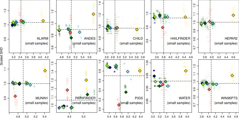
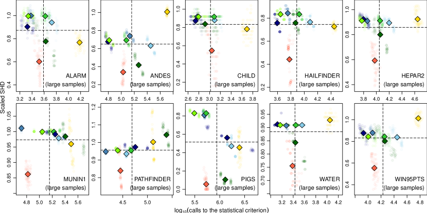
Figure 1: Scaled SHD versus speed for GS (blue), Inter-IAMB (sky blue), PC-Stable (navy blue), MMHC (green), RSMAX2 (lime green), H²PC (dark green), tabu search (red) and simulated annealing (gold) and (BIC, $\mathrm{G}^{2}_{\mathrm{BIC}}$) for the discrete BNs. Shaded points correspond to individual simulations, while diamonds are algorithm averages.

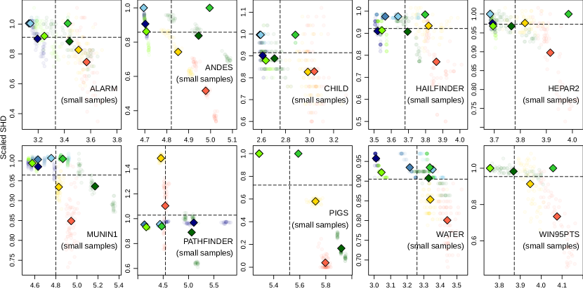
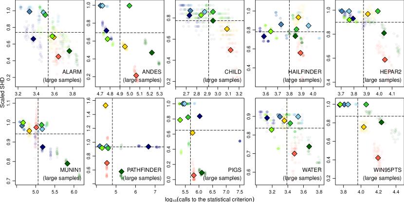
Figure 2: Scaled SHD versus speed for GS (blue), Inter-IAMB (sky blue), PC-Stable (navy blue), MMHC (green), RSMAX2 (lime green), H²PC (dark green), tabu search (red) and GES (gold) and ($\log\operatorname{P}(\mathcal{G}\operatorname{|}\mathcal{D})$, $\log\mathrm{BF}$) for the discrete BNs. Shaded points correspond to individual simulations, while diamonds are algorithm averages.

4.2 GBNs

The results for GBNs are shown in Figure 4 for (BIC, $\mathrm{G}^{2}_{\mathrm{BIC}}$), and in Figure 4 for ($\log\operatorname{P}(\mathcal{G}\operatorname{|}\mathcal{D})$, $\log\mathrm{BF}$). From the simulations with (BIC, $\mathrm{G}^{2}_{\mathrm{BIC}}$), we observe that:

• Tabu search and simulated annealing have a larger scaled SHD than both constraint-based and hybrid algorithms for all combinations of BNs and sample sizes. This can be attributed to the fact that the networks learned by tabu search and simulated annealing have a much larger number of arcs (between $10|A|$ and $2|A|$ for small samples, between $2|A|$ and $|A|$ for large samples) compared to those learned by constraint-based and hybrid algorithms (between $0.1|A|$ and $0.8|A|$ for small samples, and between $0.5|A|$ and $|A|$ for large samples); many of those arcs will be false positives and thus increase SHD.

• Constraint-based and hybrid algorithms have very similar scaled SHDs for all combinations of BNs and sample sizes.

• While scaled SHD for large samples is about 40% smaller compared to small samples for constraint-based and hybrid algorithms, tabu search and simulated annealing show a much larger improvement in accuracy (50% to 66% reduction in scaled SHD) since they start from a much worse accuracy.

• As was the case for discrete BNs, there is no consistent ranking of constraint-based and hybrid algorithms in terms of speed, PC-Stable and RSMAX2 are the two fastest algorithms in 7/8 combinations of BNs and sample sizes.

The results from the simulations performed using ($\log\operatorname{P}(\mathcal{G}\operatorname{|}\mathcal{D})$, $\log\mathrm{BF}$) paint a similar picture but for three important points:

• Due to the lack of available software, the only score-based algorithm which could be used with BGe was the tabu search implementation in bnlearn. This limits the conclusions that can be made from this set of simulations.

• Tabu search is in the bottom left quadrant (“fast, accurate”) in 7/8 combinations of BNs and sample sizes, where it is also the algorithm with the lowest scaled SHD.

• While PC-Stable is still one of the two fastest among constraint-based and hybrid algorithms in 8/8 combinations of BNs and sample size, the same is true for RSMAX2 in only 4/8 combinations.

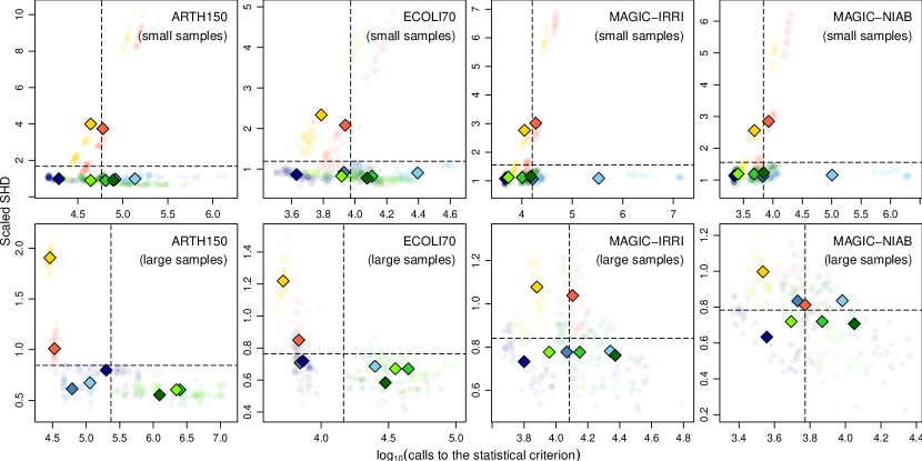
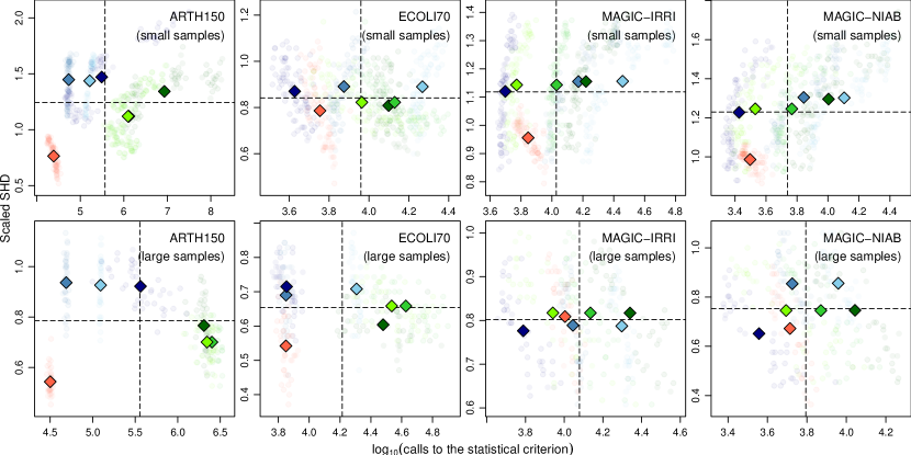
Figure 3: Scaled SHD versus speed for GS (blue), Inter-IAMB (sky blue), PC-Stable (navy blue), MMHC (green), RSMAX2 (lime green), H²PC (dark green), tabu search (red) and simulated annealing (gold) and (BIC, $\mathrm{G}^{2}_{\mathrm{BIC}}$) for the GBNs. Shaded points correspond to individual simulations, while diamonds are algorithm averages.

Figure 4: Scaled SHD versus speed for GS (blue), Inter-IAMB (sky blue), PC-Stable (navy blue), MMHC (green), RSMAX2 (lime green), H²PC (dark green), tabu search (red) and ($\log\operatorname{P}(\mathcal{G}\operatorname{|}\mathcal{D})$, $\log\mathrm{BF}$) for the GBNs. Shaded points correspond to individual simulations, while diamonds are algorithm averages.

4.3 Small Networks versus Large Networks

From the simulations above we can look into Q5 as well. For this purpose we define a “small network” as a BN with less than $50$ nodes, and a “large network” as a BN with more than $50$ nodes. Hence, the former include ALARM, CHILD, WATER, ECOLI70 and MAGIC-NIAB; and the latter include ANDES, HAILFINDER, HEPAR2, MUNIN1, PATHFINDER, PIGS, WIN95PTS, ARTH150 and MAGIC-IRRI. Making this distinction based on the number of nodes is imperfect at best, since networks of similar size can have vastly different numbers of parameters and thus very different levels of complexity. However, it provides a categorisation of networks that is intuitive to practitioners and that can be used when $|\Theta|$ is unknown. In practical applications, if we assume that the discrete BN we are trying to learn is uniformly sparse and that each variable takes at most $l$ values, each local distribution will have $O(l^{|\Pi_{X_{i}}|+1})$ parameters and we can estimate $|\Theta|$ with $O(Nl^{c+1})$ taking $|\Pi_{X_{i}}|\leqslant c$ for all $X_{i}$. As for GBNs, $|\Theta|$ is proportional to the number of arcs and can be estimated as $O(cN)$; which is even more closely aligned with the number of nodes.

Interestingly, we do not notice any systematic change in the rankings of the learning algorithms either in terms of speed or accuracy between the two groups of BNs. All the considerations we have made above for discrete BNs and GBNs hold equally for small and large networks. This is important to note because:

• Different algorithms have different computational complexities, as measured by the expected number of calls to statistical criteria with respect to $N$; which may have meant that their ranking in terms of speed might have been different between large and small networks.

• Various algorithms compute different sequences of conditional independence tests and network scores, and thus have varying levels of robustness against errors in the learning process. When the matching statistical criteria erroneously include or exclude an arc from the network, different algorithms are more or less likely to erroneously include or exclude other arcs incident on the same nodes, which may have lead to important variations in the relative speed and scaled SHDs of the algorithms.

5 Real-World Complex Data: A Climate Case Study

In this section we address Q1, Q2, Q3, Q4 and Q5 for real-world data considering a climate case study where dependencies of various orders coexist. Climate data has recently attracted a great deal of interest due to the potential application of networks to analyse the underlying complex spatial structure [53]. This includes spatial dependence among nearby locations (first-order), but also long-range (higher-order) spatial dependencies connecting distant regions in the world, known as teleconnections [54]. These teleconnections represent large-scale oscillation patterns—such as the El Niño Southern Oscillation (ENSO)—which modulate the synchronous behaviour of distant regions [55]. The most popular climate network models in the literature are complex networks [56], which are easy to build since they are based on pairwise correlations (arcs are established between pairs of stations with correlations over a given threshold) and provide topological information in the network structure (e.g. highly connected regions). BNs have been proposed as an alternative methodology for climate networks that can model both marginal and conditional dependence structures and that allows probabilistic inference [57]. However, learning BNs from complex data is computationally more demanding and choosing an appropriate structure learning algorithm is crucial. Here we consider an illustrative climate case study modelling global surface temperature. We adapt the matching score and independence test (BIC, $\mathrm{G}^{2}_{\mathrm{BIC}}$) to the family of matching scores and independence tests ($\mathrm{BIC}_{\gamma}$, $\mathrm{G}^{2}_{\mathrm{BIC}_{\gamma}}$), suitable for complex data, and we reassess the performance of the learning methods used in Section 4.

5.1 Data and Methods

We use monthly surface temperature values on a global $10^{\circ}$-resolution (approx. 1000 km) regular grid for a representative climatic period (1981 to 2010), as provided by the NCEP/NCAR reanalysis. Figure 5 shows the mean temperature (climatology) for the whole period as well as the anomaly (difference from the mean 1981-2010 climatological values) for a particular date (January 1998, representing a strong El Niño episode with high tropical Pacific temperatures).

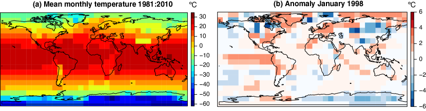
Figure 5: (a) Global mean temperature from 1981 to 2010 on a global $10^{\circ}$ grid from the NCEP reanalysis. (b) Anomaly for January 1998 (strong El Niño episode).

The surface temperature at each gridpoint is assumed to be normally distributed; hence we choose to learn GBNs in which nodes represent the (anomaly of) surface temperature at the different gridpoints and arcs represent spatial dependencies. Thus, we define $X_{i}$ as the monthly anomaly value of the temperature at location $i$ for a period of 30 years ($n=30\times 12=360$). The anomaly value is obtained by removing the mean annual cycle from the raw data (i.e. the 30-year mean monthly values) month by month. The location of a gridpoint $i$ is defined by its latitude and longitude. Hence the node set $\mathbf{X}$ in the GBN is characterised as $\mathbf{X}=\{X_{1},\dots,X_{N}\}$ with $N=18\times 36=648$.

In line with Section 4, we assess two constraint-based algorithms (PC-Stable, GS), two score-based algorithms (tabu search and hill climbing, HC) and two hybrid algorithms (MMHC, H²PC). Note, however, that in this case the sample size is fixed to what was considered a “small sample” even for a DAG with no arcs: $n/|\Theta|\leqslant 360/(648\times 2)=0.28$.

The complex spatial dependence structure of climate data is characterised by both local and distant (teleconnected) dependence patterns. Local dependencies are strong since they are the result of the short-term evolution of atmospheric thermodynamic processes. Distant teleconnected dependencies—resulting from large-scale atmospheric oscillation patterns—are in general weaker, but they are key for understanding regional climate variability. The various-order dependencies in complex data are challenging for BN structure learning algorithms and have made it necessary to introduce some adjustments in the methodology compared to Section 4. We show in Section 5.1.1 that constraint-based algorithms are problematic when using the $\mathrm{G}^{2}_{\mathrm{BIC}}$ independence test as defined in (11). To improve the performance of constraint-based algorithms for complex data we introduce below the family of extended $\mathrm{BIC}$ scores and independence tests. The extension makes constraint-based, score-based and hybrid algorithms directly comparable for complex data.

5.1.1 Limitations of Constraint-Based Algorithms: Extended BIC for Complex Data

The heuristics that underlie constraint-based algorithms (PC-Stable and GS) and the $\mathrm{G}^{2}_{\mathrm{BIC}}$ independence test, which does not enforce sparsity, are a problematic combination when learning a CPDAG from complex data. We illustrate how and where problems arise using climate data as an example. The algorithms first discover highly connected local regions and some large distance arcs (Algorithm 1, step 2). Then the algorithms attempt to identify v-structures (step 3). This is done directly, in the case of PC-Stable, by applying independence tests for two nodes with a common neighbour which is not in one of their d-separating sets; and indirectly, in the case of GS, by identifying the parents and children in the Markov blanket. In either case, since $\mathrm{G}^{2}_{\mathrm{BIC}}$ does not explicitly enforce sparsity, locally connected regions are dense (step 2) and, due to the low sample size, $\mathrm{G}^{2}_{\mathrm{BIC}}$ may also learn conflicting directions for the same arcs within each locally connected region (step 3). Even though we can try to address these conflicts with simple heuristics, such as prioritising arc directions in which $\mathrm{G}^{2}_{\mathrm{BIC}}$ shows the strongest confidence, v-structures are likely to be identified incorrectly. Furthermore, such errors are bound to cascade in step 4 when propagating arc directions to produce a final DAG. In the worst case, the algorithms may not be able to set the remaining arc directions in and between highly connected regions without creating cycles or new v-structures; an example of such a situation is shown in Figure 6. In this case the partially directed acyclic graph (PDAG) that was learned by the algorithm in step 3 does not represent an equivalence class of DAGs, and cannot be completed into a valid CPDAG in step 4. The learned PDAG does not encode any underlying probabilistic model and will be referred to as an invalid CPDAG.

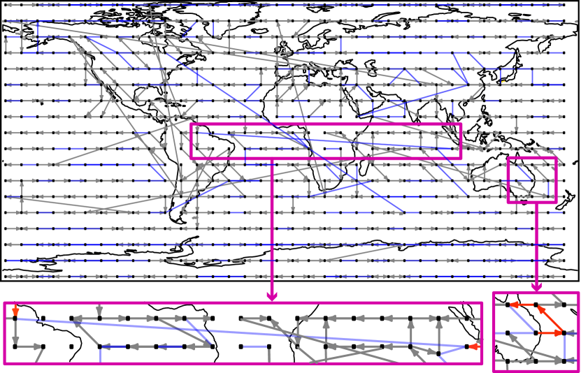
Figure 6: Partially directed graph produced by GS at the end of step 3 with BIC. Grey arcs are directed, blue arcs are undirected arcs whose directions are to be set in step 4. The bottom left panel illustrates a case in which step 4 fails to set arc directions between teleconnected regions. The bottom right panel illustrates a similar case in a highly connected region. Short-range arcs in the latter and long-distance arcs in the former can not be set in step 4 without introducing a directed cycle or a new v-structure (conflicting directions are shown in red).

In order to construct an appropriate pair of matching criteria that allow constraint-based algorithms to return valid CPDAGs for complex data, we introduce an extended version of BIC that can produce different levels of sparsity in the graph. The extended BIC comes with an additional regularisation coefficient $\gamma\in\mathbb{R}^{+}$ that penalises the number of parameters in the BN; which in turn are proportional to the number of arcs in the graph. Large values of $\gamma$ thus reduce the probability of errors in steps 3 and 4 for constraint-based algorithms. We refer to this family of scores as $\mathrm{BIC}_{\gamma}$, with $\mathrm{BIC}_{\gamma}=\mathrm{BIC}$ if $\gamma=0$, defined as

$$\mathrm{BIC}_{\gamma}(\mathcal{G};\mathcal{D})=\sum_{i=1}^{N}\left[\log\operatorname{P}(X_{i}\operatorname{|}\Pi_{X_{i}})-|\Theta_{X_{i}}|\left(\frac{\log n}{2}-\gamma\log N\right)\right].$$

We have chosen to scale $\gamma$ with the factor $|\Theta_{X_{i}}|\log N$ as in the EBIC score from [58] due to its effectiveness in feature selection. From $\mathrm{BIC}_{\gamma}$ we then construct the corresponding independence test $\mathrm{G}^{2}_{\mathrm{BIC}_{\gamma}}$ as follows:

$$\mathrm{BIC}_{\gamma}(\mathcal{G}^{+};\mathcal{D})>\mathrm{BIC}_{\gamma}(\mathcal{G}^{-};D)\Rightarrow 2\log\frac{\operatorname{P}(X_{i}\operatorname{|}\Pi_{X_{i}}\cup\{X_{j}\})}{\operatorname{P}(X_{i}\operatorname{|}\Pi_{X_{i}})}>(|\Theta_{X_{i}}^{\mathcal{G}^{+}}|-|\Theta_{X_{i}}^{\mathcal{G}^{-}}|)(2\gamma\log N+\log n).$$

In our analysis, step 4 in Algorithm 1 did not produce valid CPDAGs at all for $\gamma=0$, and not in general for every $\gamma>0$. We refer to the range of $\gamma$s for which an algorithm can return valid CPDAGs, which can then be extended into DAGs, as the parameter range of the algorithm. The matching statistical criteria ($\mathrm{BIC}_{\gamma}$, $\mathrm{G}^{2}_{\mathrm{BIC}_{\gamma}}$) allow us to compare the networks learned by all algorithms along their parameter range.

Motivated by the above, we proceed as in Section 4 but with the following changes:

1. We generate 5 permutations of the order of the variables in the data to cancel local preferences in the learning algorithms [see e.g. 20].

2. From each permutation, we learn $\mathcal{G}$ using ($\mathrm{BIC}_{\gamma}$, $\mathrm{G}^{2}_{\mathrm{BIC}_{\gamma}}$) for different values of $\gamma\in[0,50]$.

3. Since we do not have a “true” model to use as a reference, we measure the accuracy of learned BNs along the parameter range of the algorithm by their log-likelihood. We also analyse the long-distance arcs (teleconnections) established in the DAGs; and we assess their suitability for probabilistic inference by testing the conditional probabilities obtained when introducing some El Niño-related evidence. Finally we analyse the conditional dependence structure by the relative amount of unshielded v-structures in the network.

4. We measure the speed of the learning algorithms with the number of calls to the statistical criterion.

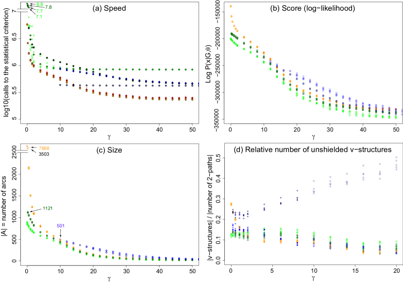
Figure 7: (a) Speed, (b) goodness of fit (log-likelihood), (c) number of arcs, (d) conditional dependence structure (unshielded v-structures) for different values of $\gamma$ learned by GS (blue), PC-Stable (navy), MMHC (green), H²PC (dark green), tabu search (red) and HC (orange). Note that orange results are on top of red ones in some cases. For clarity panel (a) includes the mean of the 5 realisation results for each $\gamma$. Labelled points in (a) have means returned by MMHC and H²PC for $\gamma\in\{0,0.2,0.5\}$ that are in speed-range higher than $7.0$. Labelled points in (c) represent the biggest networks of tabu for $\gamma\in\{0,0.2\}$ and the biggest networks found by H²PC and PC-Stable (to be analysed in Figure 8). Filled dots in (d) indicate invalid equivalence classes (CPDAGs).

5.2 Results

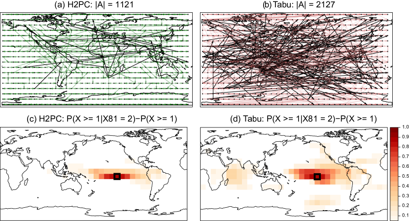
Figure 8: DAGs learned by (a) tabu search ($\gamma=0.5$) and (b) H²PC ($\gamma=0.2$). Long range links (representing teleconnections) are shown in black. (c) and (d) show the differences of the conditional and marginal probabilities obtained with both Bayesian networks after propagation of $X_{81}=2$ (denoted with a black box), simulating El Niño conditions; the graph obtained with tabu encodes well known teleconnection regions (e.g. Indian ocean) for this evidence.

Figure 7(a-c) shows the performance (speed, goodness of fit, number of arcs) of various structure learning algorithms as a function of $\gamma$, using the same colours as in Figure 4 (with the exception of hill climbing, which is new in this figure and is shown in orange). Figure 7(d) shows the conditional dependence structure (characterised by relative number of unshielded v-structures) of the CPDAGs returned by the algorithms as a function of $\gamma$. Filled dots for PC-Stable and GS denote invalid CPDAGs. Figure 7(d) is discussed separately at the end of this section. Figure 8 (a-b) shows the the two representative networks from H²PC and tabu search that are highlighted with a label in Figure 7(c) overlaid with the world map. This figure also compares the suitability of the learned BNs for probabilistic inference by propagating an El Niño-like evidence ($X_{81}=2$, i.e. warm temperatures in the corresponding gridbox in tropical Pacific).

From the networks learned with ($\mathrm{BIC}_{\gamma}$, $\mathrm{G}^{2}_{\mathrm{BIC}_{\gamma}}$) for $\gamma\in[0,50]$, we observe that:

• GS and PC-Stable produce BNs with the highest log-likelihood for large values of $\gamma$ ($\gamma\geq 10$, Figure 7(b)).

• However, GS and PC-Stable do not produce valid CPDAGs for small values of $\gamma$ ($\gamma<10$); and for $\gamma\geq 10$ they learn CPDAGs with at most $501$ arcs (smaller than the number of nodes) and no teleconnections, which are not useful for inference. (A constraint-based network is therefore excluded of Figure 8.)

• H²PC and MMHC exhibit the poorest log-likelihood values when $\gamma\geq 10$. However, in contrast with PC-Stable and GS, for $\gamma<10$ they do return valid CPDAGs resulting in a maximum number of $1121$ arcs for H²PC, including some teleconnections (Figure 8(a)).

• Inference on networks learned by hybrid and constraint-based algorithms does not highlight altered probabilities of high temperatures in the Indian Ocean when El Niño-like evidence is given (Figure 8(c), largest H²PC network). High temperatures in the Indian ocean, induced by atmospheric teleconnection, are typical when El Niño occurs as was illustrated in figure (5(b)) and found in literature[59]. The absence of a sufficient number of long-range arcs makes hybrid and constraint-based algorithms incapable to model teleconnections and therefore unsuitable for propagating evidence.

• Tabu search and HC (with almost identical results) produce networks with the highest likelihood and the largest number of arcs for $\gamma<10$ (with $|A|>2500$ for $\gamma\leq 0.2$). Even intermediate networks ($\gamma=0.5$, $|A|=2127$) include a large number of teleconnections and allow propagating evidence with realistic results (Figure 8(b,d)).

• Score-based algorithms are faster than both hybrid and constraint-based algorithms. The difference in speed with H²PC and MMHC for $\gamma\in\{0,0.2,0.5,1,1.5,2\}$ is markedly larger, because in this range the score-based algorithms return DAGs containing more arcs than the hybrids for the same $\gamma$.

Finally, in Figure 7(d) we examine the relative number of unshielded v-structures in a network, defined as the number of unshielded v-structures divided by the amount of adjacent pairs of arcs in a graph. In a DAG, on average, 25% of all adjacent pairs of arcs are (shielded or unshielded) v-structures. The proportion of unshielded v-structures is smaller and depends on $|N|$ and $|A|$. For $N=648$ and $|A|\in[25,7868]$, the average proportion of unshielded v-structures over all possible DAGs lies between $0.2499$ ($|A|=25$) and $0.2125$ ($|A|=7868$). Note that, among the DAGs we learned, those with up to 1500 arcs contain only short-range arcs and no teleconnections. It is intuitive that most pairs of adjacent arcs connecting nearby locations will not be modelled as an unshielded v-structure: they will be part of a dense cluster of nodes that are dependent just because of local weather patterns, and either the path is not a v-structure or the parents in the v-structure are likely to be connected. For a dense DAG (with more than $1500$ arcs, as returned by HC and tabu search for $\gamma\leq 0.5$) it makes sense that the amount of unshielded v-structures is higher than random as two nodes corresponding to distant geographical locations will be connected by a path of length two only when their association is strong enough to overcome the effect of local weather patterns. Results in Figure 7(d) show that all algorithms seem to follow this intuition except for PC-Stable at large values of $\gamma$ where it has the biggest relative amount of unshielded v-structures and discovers more conditional dependence structure than random.

5.3 Small Networks versus Large Networks (Climate Data)

Different classes of structure learning algorithms learn networks with different levels of sparsity when using ($\mathrm{BIC}_{\gamma}$, $\mathrm{G}^{2}_{\mathrm{BIC}_{\gamma}}$). Since the number of nodes in the networks is fixed by the geographical grid, we will treat sparse graphs as “small” and dense graphs as “large networks” because the former will have a smaller number of parameters and thus will represent simpler BNs. All algorithms are able to learn small networks with up to $500$ arcs. Hybrid and score-based algorithms can also learn medium networks with up to $1200$ arcs. Only score-based algorithms can successfully learn dense networks containing up to $8000$ arcs. Constraint-based algorithms learn the most accurate small networks in terms of log-likelihood. Score-based algorithms learn small networks faster than constraint-based algorithms and score-based algorithms learn medium networks faster and more accurately than hybrid algorithms. As score-based algorithms are the only algorithms that can model large graphs, they are the only viable choice in that case. Since only large graphs capture complex spatial dependencies we consider score-based algorithms unique in their capacity to model climate data with short- and long-range dependence structures.

6 Discussion and Conclusions

In this paper we revisited the problem of assessing different classes of BN structure learning algorithms; we improved over existing comparisons of learning accuracy and speed in the literature by removing the confounding effect of different choices of statistical criteria. Interestingly, we found that constraint-based algorithms are overall less accurate than tabu search (but not simulated annealing) for both small and large sample sizes (Q1), but are more accurate than other score-based algorithms in many simulation settings. There is no systematic difference in accuracy between constraint-based and hybrid algorithms (Q3). We also found that tabu search, as a score-based algorithm, is often faster than most constraint-based and hybrid algorithms (Q2). Finally, we found that hybrid algorithms are not faster overall than constraint-based or score-based algorithms; in fact, there was no consistent ordering of the algorithms from these classes across different simulation scenarios (Q4). We noted that PC and RSMAX2 were consistently among the fastest two constraint-based/hybrid algorithms for most of the considered BNs and sample sizes. No systematic difference in the ranking of different classes of algorithms in terms of speed and accuracy was observed for any class of algorithms for small networks compared to large networks (Q5).

All these conclusions are in contrast with other findings in the literature; among others:

• Tsamardinos et al. [37] used a set of discrete reference BNs (including ALARM, CHILD, HAILFINDER and PIGS) to compare MMHC with tabu search, GES and PC (in its original formulation from [19]). They found MMHC to be faster than tabu search ($2.34\times$) and much faster than PC ($9.22\times$), while at the same time to have a smaller SHD ($1.85\times$ larger SHD for tabu search, $7.25\times$ for PC). However, these conclusions are limited by several issues: statistical criteria in different algorithms do not match; both BDeu’s imaginary sample size and the significance threshold for the conditional independence tests are much larger than current best practices suggest [41]; sample sizes in the simulation are absolute ($n$) instead of relative ($n/\Theta$), making the aggregation of the results problematic.

• Spirtes [47] states that, unlike score-based algorithms, constraint-based algorithms “are generally fast”, but that “mistakes made early in constraint-based searches can lead to later mistakes” which is exacerbated by “the problem of multiple testing” especially in large networks.

• Similarly, Koller and Friedman [2] state that constraint-based algorithms are “sensitive to failures in individual independence tests” and that “it suffices that one of these tests return a wrong answer to mislead the network construction procedure”; while score-based algorithms are “less sensitive to individual failures” but “that they pose a search problem that may not have an elegant and efficient solution”.

• Natori et al. [48] state that constraint-based algorithms can “relax computational cost problems and can extend the available learning network size for learning” compared to score-based algorithms. In the follow-up paper [60], where they compare the Recursive Autonomy Identification (RAI) [61] constraint-based algorithm with PC (in its original formulation) and MMHC using a a set of discrete reference BNs (including ALARM, ANDES, MUNIN and WIN95PTS), they confirmed this with a simulation study in PC and RAI scale better for large networks compared to MMHC. These results, however, are problematic because speed was measured in seconds and the simulations were run with bespoke implementations of the structure learning algorithms that were heterogeneous in terms of efficiency (Matlab vs Java). In addition, the table of results in [60] is incomplete due to artificially limiting the running time of individual simulations.

• Niinimäki and Parviainen [62] compare, among other algorithms, tabu search, GES and MMHC in terms of SHD and running time (in seconds) over $4$ discrete reference BNs (HAILFINDER and modified versions of ALARM, CHILD, INSURANCE). The figures included in the paper show MMHC as being both faster and more accurate than tabu search; and to be as accurate as GES while being faster. Again the results are limited by the confounding effect of choosing different statistical criteria, and by the measuring speed in absolute running times with heterogeneous software implementations.

In addition, we note that the literature referenced in the above list provides these guidelines using only discrete BNs as a base, even when not stated explicitly. Our conclusions about the relative speed and accuracy of various classes of structure learning algorithms for GBNs is completely novel to the best of our knowledge.

For complex data we found that only score-based algorithms produce large networks in which higher-order dependencies are profoundly represented. In climate data higher-order dependencies are related to teleconnections that are key to model climate variability.

These results, which we confirmed on both simulated data and real-world complex data, are intended to provide guidance for additional studies; we do not exclude the existence of other sources of confounding, such as tuning parameters, which should be further investigated.

References

- [1] R. Cowell, Conditions Under Which Conditional Independence and Scoring Methods Lead to Identical Selection of Bayesian Network Models, in: Proceedings of the 17th Conference on Uncertainty in Artificial Intelligence, 2001, pp. 91–97.
- [2] D. Koller, N. Friedman, Probabilistic Graphical Models: Principles and Techniques, MIT Press, 2009.
- [3] D. M. Chickering, A Transformational Characterization of Equivalent Bayesian Network Structures, in: P. Besnard, S. Hanks (Eds.), Proceedings of the 11th Conference on Uncertainty in Artificial Intelligence, Morgan Kaufmann, 1995, pp. 87–98.
- [4] D. Heckerman, D. Geiger, D. M. Chickering, Learning Bayesian Networks: The Combination of Knowledge and Statistical Data, Machine Learning 20 (3) (1995) 197–243.
- [5] D. Geiger, D. Heckerman, Learning Gaussian Networks, in: Proceedings of the 10th Conference on Uncertainty in Artificial Intelligence, 1994, pp. 235–243.
- [6] C. E. Weatherburn, A First Course in Mathematical Statistics, Cambridge University Press, 1961.
- [7] G. Elidan, Copula Bayesian Networks, in: J. D. Lafferty, C. K. I. Williams, J. Shawe-Taylor, R. S. Zemel, A. Culotta (Eds.), Advances in Neural Information Processing Systems 23, 2010, pp. 559–567.
- [8] S. Moral, R. Rumi, A. Salmerón, Mixtures of Truncated Exponentials in Hybrid Bayesian Networks, in: Symbolic and Quantitative Approaches to Reasoning with Uncertainty (ECSQARU), Vol. 2143 of Lecture Notes in Computer Science, Springer, 2001, pp. 156–167.
- [9] S. L. Lauritzen, N. Wermuth, Graphical Models for Associations Between Variables, Some of which are Qualitative and Some Quantitative, The Annals of Statistics 17 (1) (1989) 31–57.
- [10] D. M. Chickering, Learning Bayesian networks is NP-Complete, in: D. Fisher, H. Lenz (Eds.), Learning from Data: Artificial Intelligence and Statistics V, Springer-Verlag, 1996, pp. 121–130.
- [11] D. M. Chickering, D. Heckerman, C. Meek, Large-sample Learning of Bayesian Networks is NP-hard, Journal of Machine Learning Research 5 (2004) 1287–1330.
- [12] T. Claassen, J. M. Mooij, T. Heskes, Learning Sparse Causal Models is not NP-hard, in: Proceedings of the 29th Conference on Uncertainty in Artificial Intelligence, 2013, pp. 172–181.
- [13] G. Schwarz, Estimating the Dimension of a Model, The Annals of Statistics 6 (2) (1978) 461–464.
- [14] F. Harary, E. M. Palmer, Graphical Enumeration, Academic Press, 1973.
- [15] R. Castelo, A. Siebes, Priors on Network Structures. Biasing the Search for Bayesian Networks, International Journal of Approximate Reasoning 24 (1) (2000) 39–57.
- [16] S. Mukherjee, T. P. Speed, Network Inference Using Informative Priors, Proceedings of the National Academy of Sciences 105 (38) (2008) 14313–14318.
- [17] G. F. Cooper, E. Herskovits, A Bayesian Method for Constructing Bayesian Belief Networks from Databases, in: Proceedings of the 7th Conference on Uncertainty in Artificial Intelligence, 1991, pp. 86–94.
- [18] T. S. Verma, J. Pearl, Equivalence and Synthesis of Causal Models, Uncertainty in Artificial Intelligence 6 (1991) 255–268.
- [19] P. Spirtes, C. Glymour, R. Scheines, Causation, Prediction, and Search, MIT Press, 2000.
- [20] D. Colombo, M. H. Maathuis, Order-Independent Constraint-Based Causal Structure Learning, Journal of Machine Learning Research 15 (2014) 3921–3962.
- [21] D. Margaritis, Learning Bayesian Network Model Structure from Data, Ph.D. thesis, School of Computer Science, Carnegie-Mellon University, Pittsburgh, PA (May 2003).
- [22] S. Yaramakala, D. Margaritis, Speculative Markov Blanket Discovery for Optimal Feature Selection, in: ICDM ’05: Proceedings of the Fifth IEEE International Conference on Data Mining, IEEE Computer Society, 2005, pp. 809–812.
- [23] C. F. Aliferis, A. Statnikov, I. Tsamardinos, S. Mani, X. D. Xenofon, Local Causal and Markov Blanket Induction for Causal Discovery and Feature Selection for Classification Part I: Algorithms and Empirical Evaluation, Journal of Machine Learning Research 11 (2010) 171–234.
- [24] R. R. Bouckaert, Bayesian Belief Networks: from Construction to Inference, Ph.D. thesis, Utrecht University, The Netherlands (1995).
- [25] P. Larrañaga, B. Sierra, M. J. Gallego, M. J. Michelena, J. M. Picaza, Learning Bayesian Networks by Genetic Algorithms: A Case Study in the Prediction of Survival in Malignant Skin Melanoma, in: Proceedings of the 6th Conference on Artificial Intelligence in Medicine in Europe (AIME’97), Springer, 1997, pp. 261–272.
- [26] S. J. Russell, P. Norvig, Artificial Intelligence: A Modern Approach, 3rd Edition, Prentice Hall, 2009.
- [27] D. M. Chickering, Optimal Structure Identification With Greedy Search, Journal of Machine Learning Research 3 (2002) 507–554.
- [28] J. Cussens, Bayesian Network Learning with Cutting Planes, in: Proceedings of the 27th Conference on Uncertainty in Artificial Intelligence, 2012, pp. 153–160.
- [29] J. Suzuki, An Efficient Bayesian Network Structure Learning Strategy, New Generation Computing 35 (1) (2017) 105–124.
- [30] M. Scanagatta, C. P. de Campos, G. Corani, M. Zaffalon, Learning Bayesian Networks with Thousands of Variables, in: Advances in Neural Information Processing Systems 28, 2015, pp. 1864–1872.
- [31] D. Madigan, J. York, Bayesian Graphical Models for Discrete Data, International Statistical Review 63 (1995) 215–232.
- [32] M. Grzegorczyk, D. Husmeier, Improving the Structure MCMC Sampler for Bayesian Networks by Introducing a New Edge Reversal Move, Machine Learning 71 (2008) 265–305.
- [33] J. Kuipers, G. Moffa, Partition MCMC for Inference on Acyclic Digraphs, Journal of the American Statistical Association 112 (517) (2017) 282–299.
- [34] P. Larrañaga, C. M. H. Kuijpers, R. H. Murga, Y. Yurramendi, Learning Bayesian Network Structures by Searching for the Best Ordering with Genetic Algorithms, IEEE Transactions on Systems, Man, and Cybernetics - Part A: Systems and Humans 26 (4) (1996) 487–493.
- [35] M. Scanagatta, G. Corani, M. Zaffalon, Improved Local Search in Bayesian Networks Structure Learning, Proceedings of Machine Learning Research (AMBN 2017) 73 (2017) 45–56.
- [36] N. Balov, P. Salzman, catnet: Categorical Bayesian Network Inference, r package version 1.15.3 (2017).
- [37] I. Tsamardinos, L. E. Brown, C. F. Aliferis, The Max-Min Hill-Climbing Bayesian Network Structure Learning Algorithm, Machine Learning 65 (1) (2006) 31–78.
- [38] M. Scutari, P. Howell, D. J. Balding, I. Mackay, Multiple Quantitative Trait Analysis Using Bayesian Networks, Genetics 198 (1) (2014) 129–137.
- [39] M. Gasse, A. Aussem, H. Elghazel, A Hybrid Algorithm for Bayesian Network Structure Learning with Application to Multi-Label Learning, Expert Systems with Applications 41 (15) (2014) 6755–6772.
- [40] A. Agresti, Categorical Data Analysis, 3rd Edition, Wiley, 2012.
- [41] M. Ueno, Learning Networks Determined by the Ratio of Prior and Data, in: Proceedings of the 26th Conference on Uncertainty in Artificial Intelligence, 2010, pp. 598–605.
- [42] J. Suzuki, A Theoretical Analysis of the BDeu Scores in Bayesian Network Structure Learning, Behaviormetrika 44 (2016) 97–116.
- [43] M. Scutari, An Empirical-Bayes Score for Discrete Bayesian Networks, Journal of Machine Learning Research (Proceedings Track, PGM 2016) 52 (2016) 438–448.
- [44] M. Scutari, Dirichlet Bayesian Network Scores and the Maximum Relative Entropy Principle, Behaviormetrika 45 (2) (2018) 337–362.
- [45] J. Kuipers, G. Moffa, D. Heckerman, Addendum on the Scoring of Gaussian Directed Acyclic Graphical Models, The Annals of Statistics 42 (4) (2014) 1689–1691.
- [46] F. Cugnata, R. S. Kenett, S. Salini, Bayesian Networks in Survey Data: Robustness and Sensitivity Issues, Journal of Quality Technology 4 (3) (2016) 253–264.
- [47] P. Spirtes, Introduction to Causal Inference, Journal of Machine Learning Research 11 (2010) 1643–1662.
- [48] K. Natori, M. Uto, Y. Nishiyama, S. K. M. Ueno, Constraint-Based Learning Bayesian Networks Using Bayes Factor, in: Advanced Methodologies for Bayesian Networks, Springer, 2015, pp. 15–31.
- [49] M. Scutari, Bayesian Network Repository, http://www.bnlearn.com/bnrepository (2012).
- [50] M. Scutari, Learning Bayesian Networks with the bnlearn R Package, Journal of Statistical Software 35 (3) (2010) 1–22.
- [51] J. A. Landsheer, The Specification of Causal Models with Tetrad IV: A Review, Structural Equation Modeling 17 (4) (2010) 703–711.
- [52] C. Wongchokprasitti, rcausal: R-Causal Library, r package version 0.99.9 (2017).
- [53] I. Fountalis, A. Bracco, C. Dovrolis, Spatio-Temporal Network Analysis for Studying Climate Patterns, Climate Dynamics 42 (3-4) (2014) 879–899.
- [54] A. A. Tsonis, K. L. Swanson, G. Wang, On the Role of Atmospheric Teleconnections in Climate, Journal of Climate 21 (12) (2008) 2990–3001.
- [55] K. Yamasaki, A. Gozolchiani, S. Havlin, Climate Networks around the Globe are Significantly Affected by El Niño, Phys. Rev. Lett. 100 (2008) 228501.
- [56] A. A. Tsonis, K. L. Swanson, P. J. Roebber, What Do Networks Have to Do with Climate?, Bulletin of the American Meteorological Society 87 (5) (2006) 585–595.
- [57] R. Cano, C. Sordo, J. M. Gutiérrez, Applications of Bayesian Networks in Meteorology, in: J. A. Gámez, S. Moral, A. Salmerón (Eds.), Advances in Bayesian Networks, Springer, 2004, pp. 309–328.
- [58] J. Chen, Z. Chen, Extended BIC For Small-n-Large-p Sparse GLM, Statistica Sinica 22 (2) (2012) 555–574.
- [59] J. B. Kajtar, A. Santoso, M. H. England, W. Cai, Tropical Climate Variability: Interactions Across the Pacific, Indian, and Atlantic Oceans, Climate Dynamics 48 (7–8) (2017) 2173–2190.
- [60] K. Natori, M. Uto, M. Ueno, Consistent Learning Bayesian Networks with Thousands of Variables, Proceedings of Machine Learning Research (AMBN 2017) 73 (2017) 57–68.
- [61] R. Yehezkel, B. Lerner, Bayesian Network Structure Learning by Recursive Autonomy Identification, Journal of Machine Learning Research 10 (2009) 1527–1570.
- [62] T. Niinimäki, P. Parviainen, Local Structure Discovery in Bayesian Networks, in: Proceedings of the 28th Conference on Uncertainty in Artificial Intelligence, 2012, pp. 634–643.