Simulations of Multiscale Schrödinger Equations with Multiscale Splitting Approaches: Theory and Application

Abstract

In this paper we present a novel multiscale splitting approach to solve multiscale Schrödinger equation, which have large different time-scales. The energy potential is based on highly oscillating functions, which are magnitudes faster than the transport term. We obtain a multiscale problem and a highly stiff problem, while standard solvers need to small time-steps. We propose multiscale solvers, which are based on operator splitting methods and we decouple the diffusion and reaction part of the Schrödinger equation. Such a decomposition allows to apply a large time step for the implicit time-discretization of the diffusion part and small time steps for the explicit and highly oscillating reaction part. With extrapolation steps, we could reduce the computational time in the highly-oscillating time-scale, while we relax into the slow time-scale. We present the numerical analysis of the extrapolated operator splitting method. First numerical experiments verified the benefit of the extrapolated splitting approaches.

Keywords: Schrödinger equation, multiscale splitting approaches, operator splitting, extrapolation methods, blow-up problem, oscillating problem.

AMS subject classifications. 35K25, 35K20, 74S10, 70G65.

1 Introduction

The Schrödinger Equation is wel-known for modelling the basis of quantum mechanics. The state of a particle is described by its wave-function $\Psi$, which is a function of space (position) $x$ and time $t$. The wave-function is given as a complex variable and it is delicate to attribute any distinct physical meaning to such complex notation. We consider a delicate multiscale problem based on different time-scales in the diffusion and reaction part of the time-dependent Schrödinger equation, see [15], [10] and [13]. Based on the large scale-dependencies, we have to apply time-restrictions to the numerical methods, see [11], such that we apply multiscale methods to decompose the different scales and accelerate the solver process. We propose novel multiscale methods, which are based on AB-splitting and ABA-splitting methods, see [4] and [5], and additional modification with extrapolation and averaging ideas. We also test heterogeneous multiscale methods (HMM), see [3] and apply the ideas of the equation-free methods (EFM), see [12]. We compare the different novel splitting approaches with the standard splitting schemes, see also [9]. Such combinations allow to overcome the delicate stiffness problems of the scale-dependent Schrödinger equation and reduce the computational time.

The paper is outlined as following. The model is introduced in Section 2. In Section 3, we discuss the different numerical methods and present the convergence analysis. The numerical experiments are done in Section 4 and the conclusion is presented in Section 5.

2 Mathematical Model

In the following, we deal with the multiscale Schrödinger equation, which is given for the first dimension as:

$$i\;\epsilon\frac{\partial\Psi}{\partial t}=-\epsilon^{2}\frac{\partial^{2}}{\partial x^{2}}\Psi+V(x)\Psi,$$ (1)

$$\frac{\partial\Psi}{\partial t}=i\;\epsilon\frac{\partial^{2}}{\partial x^{2}}\Psi-i\;\frac{1}{\epsilon}V(x)\Psi,$$ (2)

where $\epsilon\in(0,1)$, $V(x)$ is the potential, e.g., $x^{2}$ or $\sin(2\pi x)$ or $\exp(\sin(2\pi x))$.

He, we assume the connection to the instationary Schrödinger equation, which is given if we apply $\hbar\rightarrow\epsilon$ and $\frac{\hbar^{2}}{m}\rightarrow\epsilon^{2}$.

For the different numerical schemes, we deal with two equations:

• Scaled equation (test example)
  In the following, we apply a scaled Schrödinger equation with $\epsilon$, where we scale $L=1.0$, therefore $\epsilon\in[10^{-6},10^{-3}]$.

  $$i\epsilon\frac{\partial\Psi(x,t)}{\partial t} =-\epsilon^{2}\frac{\partial^{2}\Psi(x,t)}{\partial x^{2}}+V(x)\Psi(x,t),$$ (3)

  $$\frac{\partial\Psi(x,t)}{\partial t} =i\;\epsilon\frac{\partial^{2}\Psi(x,t)}{\partial x^{2}}-\frac{i}{\epsilon}V(x)\Psi(x,t),$$ (4)

  where the initial condition is given as $\Psi(x,0)=sin(\pi x)$ with $x\in[0,1]$ and $t\in[0,1]$.

• Unscaled equation (full Schrödinger equation)

  $$i\hbar\frac{\partial}{\partial t}\Psi(x,t)=\hat{H}\Psi(x,t),$$ (5)

  $$\frac{\partial}{\partial t}\Psi(x,t)=-i\;\frac{1}{\hbar}\hat{H}\Psi(x,t),$$ (6)

  where $\hat{H}=-\frac{\hbar^{2}}{2\mu}\nabla^{2}+V(x,t)$.
  We apply the initial conditions:
  $\Psi(x,0)=\exp(-0.5(\frac{x-x_{c}}{s})^{2})cos(\frac{2\pi(x-x_{c})}{\lambda})+i\exp(-0.5(\frac{x-x_{c}}{s})^{2})sin(\frac{2\pi(x-x_{c})}{\lambda})$, where $x\in[0,L]$, where we have $L=4\;10^{-9}\;[m]$, $\lambda=L/40$ and $s=L/25$.

  Further, we assume $V(x,t)=0$ and $V(x,t)=e\;x^{2}$,
  where $e=1.6021766\;10^{-19}\;[C]$ is the charge of the electron.

Remark 1

The instationary Schrödinger equation is given as:

$$i\hbar\frac{\partial}{\partial t}\Psi(x,t)=\hat{H}\Psi(x,t),$$ (7)

$$\frac{\partial}{\partial t}\Psi(x,t)=-i\;\frac{1}{\hbar}\hat{H}\Psi(x,t),$$ (8)

where $\hat{H}=-\frac{\hbar^{2}}{2\mu}\nabla^{2}+V(x,t)$. further $\mu$ is the particle’s reduced mass, $i$ is imaginary unit, V(x,t) is its potential energy, $\nabla^{2}$ is the Laplacian (a differential operator), and $\Psi$ is the wave function. The instationary Schrödinger equation can be rewritten with respect to an $\epsilon$-parameter to a multiscale Schrödinger equation, see Equation (1) and (2).

3 Numerical methods

In the following, we present the different splitting methods, which are discussed as:

• Standard operator splitting methods:

  • AB-splitting method or Lie-Trotter splitting method, see [16], which solve each operator in a separate equation and apply different time-steps for each operator.

  • ABA-splitting or BAB-splitting method or Strang splitting method, see [14], which improves the AB-splitting method with respect to additional steps for the separated operators. Further, we also assume to deal with the different time-steps for each operator.

• Modified multiscale splitting methods.

  • HMM-AB-splitting method, see [9], which combines the Heterogeneous Multiscale method and the AB-splitting method, such that we could embed the microscopic operator equation with a smaller amount of microscopic time-steps into the macroscopic operator equation.

  • Extrapolated AB-splitting method, see the ideas in [12], which combines the equation free methods and the AB-splitting method. Therefore, we could reduce the large amount of microscopic time-steps of the microscopic operator equation and apply extrapolation methods and embed the results into the macroscopic operator equation.

  • Higher-Order Extrapolated ABA-splitting method, see the ideas in [12], here we combine higher order extrapolation methods and ABA-splitting method. Therefore, we could reduce the large amount of microscopic time-steps of the microscopic operator equation and apply extrapolation methods and embed the results into the macroscopic operator equation. Further, we also obtain a second order scheme.

3.1 Instationary Schrödinger equation

We discretize the instationary Schrödinger equation (7) with implicit time-discretization and second order spatial discretization methods.

The discretization is given as:

$$i\hbar\frac{\Psi(x,t)-\Psi(x,t-\Delta t)}{\Delta t} =-\frac{\hbar^{2}}{2m}\frac{\Psi(x+\Delta x,t)-2\Psi(x,t)+\Psi(x-\Delta x,t)}{\Delta x^{2}}+$$ (9)

$$+V(x,t)\Psi(x,t),$$

where we obtain:

$$\frac{\Psi(x,t)-\Psi(x,t-\Delta t)}{\Delta t} =i\frac{\hbar}{2m}\frac{\Psi(x+\Delta x,t)-2\Psi(x,t)+\Psi(x-\Delta x,t)}{\Delta x^{2}}-$$ (10)

$$-\frac{i}{\hbar}V(x,t)\Psi(x,t).$$

Then, we simplify the discretized Equation (10) and obtain:

$$\Psi(x,t-\Delta t) =-\frac{i\;\hbar\Delta t}{2m\Delta x^{2}}(\Psi(x+\Delta x,t)-2\Psi(x,t)+$$ (11)

$$+\Psi(x-\Delta x,t))+(1+\frac{i\;\Delta tV(x,t)}{\hbar})\Psi(x,t).$$

Then, we rewrite the Equation (11) in a matrix-notation, which can be programmed to software-package, e.g., MATLAB^®:

$$\Psi(k-1)=-\frac{i\;\hbar\Delta t}{2m\Delta x^{2}}\begin{bmatrix}-2&1&0&0&\dots&0\\ 1&-2&1&0&\dots&0\\ 0&1&-2&1&\dots&0\\ \vdots&\vdots&\vdots&\vdots&\ddots&\vdots\\ 0&0&0&0&\dots&-2\end{bmatrix}\Psi(k)$$ (12)

$$+\begin{bmatrix}(1+\frac{i\;\Delta tV(x_{0},t)}{\hbar})&0&0&0&\dots&0\\ 0&(1+\frac{i\;\Delta tV(x_{2},t)}{\hbar})&0&0&\dots&0\\ 0&0&(1+\frac{i\;\Delta tV(x_{3},t)}{\hbar})&0&\dots&0\\ \vdots&\vdots&\vdots&\vdots&\ddots&\vdots\\ 0&0&0&0&\dots&(1+\frac{i\;\Delta tV(x_{M},t)}{\hbar})\end{bmatrix}\Psi(k),$$

where $j=0,1,\ldots,J$ are the spatial points with $\Delta x=1/J$ and $x_{j}=j\;\Delta x$. Then, we obtain the operator equation:

$$\Psi(k-1)=\textbf{B}\Psi(k),$$ (13)

$$\Psi(k)=\mathbf{B}^{-1}\Psi(k-1).$$ (14)

Remark 2

The standard finite difference discretization with implicit
time-discretization and second order spatial discretization leads to large linear equation systems. Here, we do not separate the operators with respect to their different time-steps, such that we solve a stiff equation system and neglect the microscopic operator, see [2] and [7].

3.2 AB and ABA Splitting for the Multiscale Schrödinger equation

We apply the following idea AB splitting method, while the diffusion operator is implicit discretized in time (large time steps) and the potential operator (reaction operator) is explicit discretized in time.

We apply the following discretization in time and space with the point $(x,t)$ as:

$$(1-\frac{i\;\Delta tV(x)}{\epsilon})\Psi(x,t-\Delta t)=$$

$$=\Psi(x,t)-\frac{i\;\epsilon\Delta t}{\Delta x^{2}}(\Psi(x+\Delta x,t)-2\Psi(x,t)+\Psi(x-\Delta x,t)).$$ (15)

Then, we have the semi-discretized operator equation as:

$$(I-\Delta t\textbf{A}_{1})\Psi(k-1) =(I+\Delta t\textbf{A}_{2})\Psi(k),$$ (16)

$$\textbf{B}_{1}\Psi(k-1) =\textbf{B}_{2}\Psi(k),$$ (17)

where the potential matrix is $\textbf{B}_{1}=\begin{bmatrix}1-\tilde{a}_{0}&0&0&0&\dots&0\\ 0&1-\tilde{a}_{1}&0&0&\dots&0\\ 0&0&1-\tilde{a}_{2}&0&\dots&0\\ \vdots&\vdots&\vdots&\vdots&\ddots&\vdots\\ 0&0&0&0&\dots&1-\tilde{a}_{M}\end{bmatrix},$

with $\tilde{a}_{j}=\frac{i\;\Delta tV(x_{j})}{\epsilon}$ and
and the diffusion matrix is $\textbf{B}_{2}=\begin{bmatrix}1+2a&-a&0&0&\dots&0\\ -a&1+2a&-a&0&\dots&0\\ 0&-a&1+2a&-a&\dots&0\\ \vdots&\vdots&\vdots&\vdots&\ddots&\vdots\\ 0&0&0&0&\dots&1+2a\end{bmatrix},$

with $a=\frac{i\;\epsilon\Delta t}{\Delta x^{2}}$.

We have the AB-splitting method as:

$$u_{1}(k)=\textbf{B}_{1}\Psi(k-1),$$ (18)

$$\Psi(k)=(\textbf{B}_{2})^{-1}u_{1}(k).$$ (19)

Based on the small scale of operator $\textbf{B}_{1}$, we improve as:

$$u_{1}(k-1,m+1)=\tilde{\textbf{B}}_{1}\Psi(k-1,m),$$ (20)

with $\tilde{\textbf{B}}_{1}=\begin{bmatrix}1-\tilde{\tilde{a}}_{0}&0&0&0&\dots&0\\ 0&1-\tilde{\tilde{a}}_{1}&0&0&\dots&0\\ 0&0&1-\tilde{\tilde{a}}_{2}&0&\dots&0\\ \vdots&\vdots&\vdots&\vdots&\ddots&\vdots\\ 0&0&0&0&\dots&1-\tilde{\tilde{a}}_{M}\end{bmatrix},$

with $\tilde{\tilde{a}}_{j}=\frac{i\;\delta tV(x_{j})}{\epsilon}$.

Further, we have $m=0,\ldots,M-1$ and $\delta t=\frac{\Delta t}{M}$ with $M=\frac{1}{\epsilon}$ and $M$ is assumed to be an integer. We have $\Psi(k-1,0)=\Psi(k-1)$ as the initialization and $\Psi(k)=\Psi(k-1,M)$ as the result.

The algorithm is given as:

$$u_{1}(k)=(\tilde{\textbf{B}}_{1})^{M}\Psi(k-1),$$ (21)

$$\Psi(k)=(\textbf{B}_{2})^{-1}u_{1}(k),$$ (22)

where $M$ is the number of intermediate time steps in the microscopic scale means $\delta t=\Delta t/M$.

The AB splitting method is given in Algorithm 3.1 as:

Algorithm 3.1

• Step 1: Solving the microscopic equation (potential part):

  $$u_{1}(t^{n+1})=(\tilde{\textbf{B}}_{1})^{M}\Psi(t^{n}),$$ (23)

  with $\tilde{\textbf{B}}_{1}$ is the discretized potential operator (small scale) and $M$ is the number of small time steps with $\delta t=\Delta t/M$.

• Step 2: Solving the macroscopic equation (diffusion part)

  $$\Psi(t^{n+1})=(\textbf{B}_{2})^{-1}u_{1}(t^{n+1}),$$ (24)

  with $\textbf{B}_{2}$ is the discretized diffusion operator (large scale).

Remark 3

For the ABA and BAB methods, we have socalled three step methods, while we apply for example the A operator with the $\Delta t/2$ timestep (at least 2 times, means at the step 1 and step 3) and the one time the $\Delta t$ timestep for B.

The ABA splitting method is given in Algorithm 3.2 as:

Algorithm 3.2

• Step 1: Solving the microscopic equation (potential part):

  $$u_{1}(t^{n+1})=(\tilde{\textbf{B}}_{1})^{M}\Psi(t^{n}),$$ (25)

  with $\tilde{\textbf{B}}_{1}$ is the discretized potential operator (small scale) and $M$ is the number of small time steps with $\delta t=(\Delta t/2)/M$.

• Step 2: Solving the macroscopic equation (diffusion part)

  $$u_{2}(t^{n+1})=(\textbf{B}_{2})^{-1}u_{1}(t^{n+1}),$$ (26)

  with $\textbf{B}_{2}$ is the discretized diffusion operator (large scale).

• Step 3: Solving the microscopic equation (potential part):

  $$\Psi(t^{n+1})=(\tilde{\textbf{B}}_{1})^{M}u_{2}(t^{n+1}),$$ (27)

  with $\tilde{\textbf{B}}_{1}$ is the discretized potential operator (small scale) and $M$ is the number of small time steps with $\delta t=(\Delta t/2)/M$.

The BAB splitting method is given in Algorithm 3.3, where we have the first B-step with $(B_{2})^{-1}$ and $\Delta t/2$, then the A-step with $(\tilde{B}_{1})^{M}$ and time-step $\delta t=\Delta t/M$ and the second B-step with $(B_{2})^{-1}$ with $\Delta t/2$.

Algorithm 3.3

• Step 1: Solving the macroscopic equation (diffusion part) with a half time step $\Delta t/2$

  $$u_{1}(t^{n+1})=(\textbf{B}_{2})^{-1}\phi(t^{n}),$$ (28)

  with $\textbf{B}_{2}$ is the discretized diffusion operator (large scale) with the half time-step means $\Delta t/2$.

• Step 2: Solving the microscopic equation (potential part):

  $$u_{2}(t^{n+1})=(\tilde{\textbf{B}}_{1})^{M}u_{1}(t^{n+1}),$$ (29)

  with $\tilde{\textbf{B}}_{1}$ is the discretized potential operator (small scale) and $M$ is the number of small time steps with $\delta t=\Delta t/M$.

• Step 3: Solving the macroscopic equation (diffusion part) with a next half time-step $\Delta t/2$

  $$\phi(t^{n+1})=(\textbf{B}_{2})^{-1}u_{2}(t^{n+1}),$$ (30)

  with $\textbf{B}_{2}$ is the discretized diffusion operator (large scale) with the half time-step means $\Delta t/2$.

Remark 4

Here, we have the stability condition with respect for reaction term, which is give as:

$$\delta t\leq\frac{\epsilon}{V(x)},$$ (31)

where $V(x)=e\;x^{2}$ is a very small number, such that we only have a critical time-step, if we assume $\epsilon\approx e$, then we have to deal with small time-steps.

Remark 5

Based on the operator splitting methods, see also [4] and [6], we have the following splitting errors:

• AB-splitting:

  $$err_{AB,local}(\Delta t)\leq\Delta t^{2}C_{AB},$$ (32)

  where the constant $C_{AB}$ is depending of $\|(\textbf{A}_{1}\|$, $\|(\textbf{A}_{2}\|$, see [6].

• AB-splitting:

  $$err_{ABA,local}(\Delta t)\leq\Delta t^{3}C_{ABA},$$ (33)

  where the constant $C_{ABA}$ is depending of $\|(\textbf{A}_{1}\|$, $\|(\textbf{A}_{2}\|$, see [6].

Further $\|\cdot\|$ is an appropriated matrix norm in the appropriate Hilbert-space.

3.3 Modified Multiscale AB for the Multiscale Schrödinger equation

We start with the discretization of the multiscale Schrödinger equation (1) and (2).

We modify the small scale of operator $\textbf{B}_{1}$ as following:

$$u_{1}(k-1,m+1)=\tilde{\textbf{B}}_{1}\Psi(k-1,m),$$ (34)

where $m=0,\ldots,M-1$ and $\delta t=\frac{\Delta t}{M}$ with $M=\frac{1}{\epsilon}$ and $M$ is assumed to be an integer. We have $\Psi(k-1,0)=\Psi(k-1)$ as the initialisation and $\Psi(k)=\Psi(k-1,m)$ with $m=1,\ldots,\tilde{M}$ the successor results with $\tilde{M}\leq M$.

We have the following multiscale AB algorithms:

1. Full-AB:
   The algorithm is given as:

   $$u_{1}(k)=(\tilde{\textbf{B}}_{1})^{M}\Psi(k-1),$$ (35)

   $$\Psi(k)=(\textbf{B}_{2})^{-1}u_{1}(k),$$ (36)

   where $M$ is the number of intermediate time steps in the microscopic scale means $\delta t=\Delta t/M$. Here, we applied the full time-interval.

2. HMM-AB:
   The algorithm is given as:

   $$u_{1}(k-1,m)=(\tilde{\textbf{B}}_{1})^{m}\Psi(k-1),\;\mbox{for}\;m=1,\ldots,\tilde{M},$$ (37)

   $$u_{1}(k)=\frac{1}{\tilde{M}}\;\sum_{m=1}^{\tilde{M}}u_{1}(k-1,m),$$ (38)

   $$\Psi(k)=(\textbf{B}_{2})^{-1}u_{1}(k),$$ (39)

   where $M$ is the number of intermediate time steps in the microscopic scale means $\delta t=\Delta t/M$.
   

3. Extrapolated-AB:
   The algorithm is given as:

   $$u_{1}(k-1,\tilde{M}-1)=(\tilde{\textbf{B}}_{1})^{\tilde{M}-1}\Psi(k-1),$$ (40)

   $$u_{1}(k-1,\tilde{M})=(\tilde{\textbf{B}}_{1})^{\tilde{M}}\Psi(k-1),$$ (41)

   $$u_{1}(k)=u_{1}(k-1,\tilde{M}-1)+$$

   $$+(\Delta t-\delta t\;(\tilde{M}-1))\frac{u_{1}(k-1,\tilde{M})-u_{1}(k-1,\tilde{M}-1)}{\delta t},$$ (42)

   $$\Psi(k)=(\textbf{B}_{2})^{-1}u_{1}(k),$$ (43)

   where $M$ is the number of intermediate time steps in the microscopic scale means $\delta t=\Delta t/M$.

4. Higher-order Extrapolated-AB:
   The algorithm is given as:

   $$u_{1}(k-1,\tilde{M}-1)=(\tilde{\textbf{B}}_{1})^{\tilde{M}-1}\Psi(k-1),$$ (44)

   $$u_{1}(k-1,\tilde{M}-2)=(\tilde{\textbf{B}}_{1})^{\tilde{M}-2}\Psi(k-1),$$ (45)

   $$u_{1}(k-1,\tilde{M})=(\tilde{\textbf{B}}_{1})^{\tilde{M}}\Psi(k-1),$$ (46)

   $$u_{1}(k)=u_{1}(k-1,\tilde{M}-1)+$$

   $$+(\Delta t-\delta t\;(\tilde{M}-1))\frac{u_{1}(k-1,\tilde{M})-u_{1}(k-1,\tilde{M}-1)}{\delta t}+$$

   $$+\frac{(\Delta t-\delta t\;(\tilde{M}-1))^{2}}{2}\cdot$$

   $$\cdot\frac{(u_{1}(k-1,\tilde{M})-2u_{1}(k-1,\tilde{M}-1)+u_{1}(k-1,\tilde{M}-2))}{(\delta t)^{2}},$$ (47)

   $$\Psi(k)=(\textbf{B}_{2})^{-1}u_{1}(k),$$ (48)

   where $M$ is the number of intermediate time steps in the microscopic scale means $\delta t=\Delta t/M$.

5. Higher-order Extrapolated-ABA:
   The algorithm is given as:

   $$u_{1}(k-1,\tilde{M}-1)=(\tilde{\textbf{B}}_{1})^{\tilde{M}-1}\Psi(k-1),$$ (49)

   $$u_{1}(k-1,\tilde{M}-2)=(\tilde{\textbf{B}}_{1})^{\tilde{M}-2}\Psi(k-1),$$ (50)

   $$u_{1}(k-1,\tilde{M})=(\tilde{\textbf{B}}_{1})^{\tilde{M}}\Psi(k-1),$$ (51)

   $$u_{1}(k)=u_{1}(k-1,\tilde{M}-1)+$$

   $$+(\Delta t-\delta t\;(\tilde{M}-1))\frac{u_{1}(k-1,\tilde{M})-u_{1}(k-1,\tilde{M}-1)}{\delta t}+$$

   $$+\frac{(\Delta t-\delta t\;(\tilde{M}-1))^{2}}{2}\cdot$$

   $$\cdot\frac{(u_{1}(k-1,\tilde{M})-2u_{1}(k-1,\tilde{M}-1)+u_{1}(k-1,\tilde{M}-2))}{(\delta t)^{2}},$$ (52)

   $$u_{2}(k)=(\textbf{B}_{2})^{-1}u_{1}(k),$$ (53)

   $$u_{3}(k-1,\tilde{M}-1)=(\tilde{\textbf{B}}_{1})^{\tilde{M}-1}u_{2}(k),$$ (54)

   $$u_{3}(k-1,\tilde{M}-2)=(\tilde{\textbf{B}}_{1})^{\tilde{M}-2}u_{2}(k),$$ (55)

   $$u_{3}(k-1,\tilde{M})=(\tilde{\textbf{B}}_{1})^{\tilde{M}}u_{2}(k),$$ (56)

   $$\Psi(k)=u_{3}(k-1,\tilde{M}-1)+$$ (57)

   $$+(\Delta t-\delta t\;(\tilde{M}-1))\frac{u_{3}(k-1,\tilde{M})-u_{3}(k-1,\tilde{M}-1)}{\delta t}+$$

   $$+\frac{(\Delta t-\delta t\;(\tilde{M}-1))^{2}}{2}\cdot$$

   $$\cdot\frac{(u_{3}(k-1,\tilde{M})-2u_{3}(k-1,\tilde{M}-1)+u_{3}(k-1,\tilde{M}-2))}{(\delta t)^{2}},$$

   where $M$ is the number of intermediate time steps in the microscopic scale means $\delta t=(\Delta t/2)/M$.

In the following, we have the remark to the extrapolation methods, see Remark 6.

Remark 6

We assume to compute $u^{n+1}$ and apply the Taylor-expansion as following:

$$u(t^{n+1})=u(t^{n})+\Delta t\frac{\partial u}{\partial t}|_{t^{n}}+\frac{\Delta t^{2}}{2!}\frac{\partial^{2}u}{\partial t^{2}}|_{t^{n}}+\frac{\Delta t^{3}}{3!}\frac{\partial^{2}u}{\partial t^{2}}|_{t^{n}}+\ldots,$$ (58)

where $\Delta t=t^{n+1}-t^{n}$.

We assume to deal with finer time-steps $\delta t=\Delta t/M$ and we have computed a series of finer resolutions $u(t^{n},m)$ with $m=1,\ldots,\tilde{M}$ and the initialisation $u(t^{n},0)=u(t^{n})$.

Then we can apply the extrapolation:

$$u(t^{n+1})\approx u(t^{n},\tilde{M}-1)+$$ (59)

$$+(\Delta t-\delta t\;(\tilde{M}-1))\frac{u(t^{n},\tilde{M})-u(t^{n},\tilde{M}-1)}{\delta t},$$

$$+\frac{(\Delta t-\delta t\;(\tilde{M}-1))^{2}}{2!}\;\frac{(u(t^{n},\tilde{M})-2u(t^{n},\tilde{M}-1)+u(t^{n},\tilde{M}-2))}{(\delta t)^{2}}+\mathcal{O}(\delta t^{3}).$$

where we obtain an global error based on $\mathcal{O}(\delta t^{2})$.

3.4 Numerical Analysis of the extrapolated AB splitting method

In the following, we analyze the consistence and order of the extrapolated AB-splitting method (40)–(43) and the higher extrapolated AB-splitting method (49)–(57).

We assume, we have linear bounded operators $A_{1},A_{2}:\!{{\bf X}}\rightarrow{{\bf X}}$, which are semi-discretized with finite difference schemes of the multiscale Schrödinger equation given in (3)-(4).

Theorem 3.4

Let $A_{1},A_{2}\in{\mathcal{L}(X)}$ are given linear bounded operators and we consider the abstract Cauchy problem

$$\begin{array}[]{c}{\displaystyle\partial_{t}c(t)=Ac(t)+Bc(t),\quad 0<t\leq T}\\ \vskip 4.30554pt\cr{\displaystyle c(0)=c_{0}.}\end{array}$$ (60)

Then the problem (60) has a unique solution.

We apply the extrapolated AB-splitting method (40)–(43) and the higher extrapolated AB-splitting method (49)–(57) with uniform macroscopic time-steps $\Delta t=t^{n+1}-t^{n}$ with $n=0,\ldots,N$. The time-interval is $[0,T]$ and we have $t^{N+1}=T$ and $t^{0}=0$.

Then, we have the following convergence results:

1. Extrapolated AB splitting method: The local convergence is given as $(C_{AB}+C_{extrapol})\delta t^{2}$, where $C_{AB}$ and $C_{extrapol}$ are bounded constants. The global convergence of the extrapolated AB splitting method is given as $\mathcal{O}(\delta t)$ and $\Delta t=M\delta t$ is the microscopic time-step.

2. Higher Extrapolated ABA splitting method: The local convergence is given as $(C_{ABA}+C_{highextra})\delta t^{3}$, where $C_{ABA}$ and $C_{highextra}$ are bounded constants. The global convergence of the extrapolated AB splitting method is given as $\mathcal{O}(\delta t^{2})$ and $\Delta t/2=M\delta t$ is the microscopic time-step.

Proof

1. Convergence of the extrapolated AB splitting method:
   We have the following local error function $E(\Delta t,\delta t)=u(t)-u_{extrapolAB}(t)$, where $\Delta t=t^{n+1}-t^{n}$ and $\delta t=\Delta t/M$ we have the relations

   $$||u(t)-u_{extrapolAB}(t)||\leq$$ (61)

   $$\leq||u(t)-u_{AB}(t)+u_{AB}(t)-u_{extrapolAB}(t)||,$$

   we know, that the splitting error of an AB-splitting is given in Remark (5) with:

   $$||u(t^{n+1})-u_{AB}(t^{n+1})||\leq C_{AB}\Delta t^{2}||u(t^{n})||.$$ (62)

   Further, the error of the first order extrapolation method is given as, see Remark 6

   $$||u_{AB}(t^{n+1})-u_{extrapolAB}(t^{n+1})||\leq C_{extrapol}\delta t^{2}||u(t^{n})||.$$ (63)

   Then, we obtain:

   $$||u(t^{n+1})-u_{extrapolAB}(t^{n+1})|| \leq C_{AB}\Delta t^{2}+C_{extrapol})\delta t^{2}$$ (64)

   $$\leq(C_{AB}M^{2}+C_{extrapol})\delta t^{2}||u(t^{n})||.$$

   Further the global error is given as:

   $$E_{global}(T) =(N+1)M||E(\Delta t,\delta t)||=$$

   $$=(N+1)M\delta t||\frac{E(\Delta t,\delta t)}{\delta t}||\leq\mathcal{O}(\delta t).$$

2. Convergence of the higher extrapolated ABA splitting method:
   We have the following local error function $E_{ABA}(\Delta t,\delta t)=u(t)-u_{extrapolABA}(t)$, where $\Delta t=t^{n+1}-t^{n}$ and $\delta t=(\Delta t/2)/M$ we have the relations

   $$||u(t)-u_{extrapolABA}(t)||\leq$$ (66)

   $$\leq||u(t)-u_{ABA}(t)+u_{ABA}(t)-u_{extrapolABA}(t)||,$$

   we know, that the splitting error of an AB-splitting is given in Remark (5) with:

   $$||u(t^{n+1})-u_{ABA}(t^{n+1})||\leq C_{ABA}\Delta t^{3}||u(t^{n})||.$$ (67)

   Further, the error of the second order extrapolation method is given as, see Remark 6

   $$||u_{ABA}(t^{n+1})-u_{extrapolABA}(t^{n+1})||\leq C_{higherextra})\delta t^{3}||u(t^{n})||.$$ (68)

   Then, we obtain:

   $$||u(t^{n+1})-u_{extrapolABA}(t^{n+1})||\leq C_{ABA}\Delta t^{2}+C_{higherextra})\delta t^{3}$$

   $$\leq(C_{ABA}(2M)^{2}+C_{extrapol})\delta t^{3}||u(t^{n})||.$$ (69)

   Further the global error is given as:

   $$E_{global}(T) =(N+1)2M||E_{ABA}(\Delta t,\delta t)||=$$

   $$=(N+1)2M\delta t||\frac{E_{ABA}(\Delta t,\delta t)}{\delta t}||\leq\mathcal{O}(\delta t^{2}).$$

Remark 7

If we apply of higher order splitting schemes, e.g., ABA splitting method, for the multiscale solver, we also need higher order extrapolation schemes. Therefore, we have taken into account higher order extrapolation schemes for improved splitting approaches.

4 Numerical Experiments

In the following experiment, we test the multiscale solver methods for the one-dimensional timedependent Schrödinger equation with a highly oscillating potential.

4.1 Test example 1

For the instationary Schrödinger equation, which is given in Equation (1), we test the following methods:

• Finite difference scheme for multiscale Schrödinger equation (unsplitted),

• AB splitting for the multiscale Schrödinger equation,

• HMM for the multiscale Schrödinger equation.

We apply the initial conditions:
$\Psi(x,0)=\exp(-0.5(\frac{x-x_{c}}{s})^{2})cos(\frac{2\pi(x-x_{c})}{\lambda})+i\;\exp(-0.5(\frac{x-x_{c}}{s})^{2})sin(\frac{2\pi(x-x_{c})}{\lambda})$, where $x\in[0,L]$, where we have $L=4\;10^{-9}\;[m]$, $\lambda=L/40$ and $s=L/25$.

Further, we assume $V(x,t)=0$ and $V(x,t)=e\;x^{2}$,
where $e=1.6021766\;10^{-19}\;[C]$ is the charge of the electron. We apply for all the methods implicit time-discretization methods and restrict us to the time-step based on the smallest time-scale. We apply therefore $\Delta x=10^{-12}$ and $\Delta t=10^{-20}$.

In Figure 1, we have the numerical results of the multiscale Schrödinger equation with finite difference scheme (without splitting). This method, we apply for a reference solution.

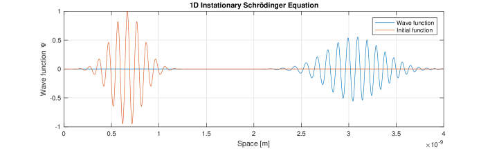
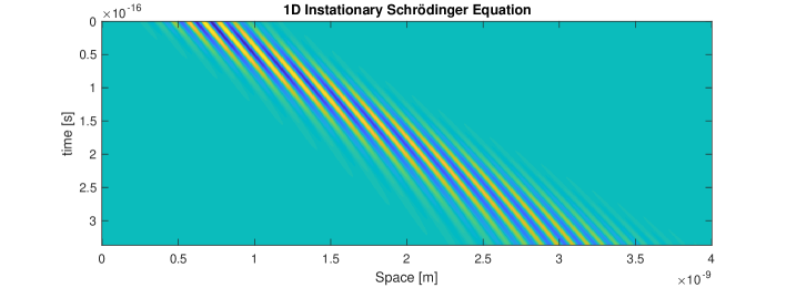
Figure 1: Simulations with the instationary Schrödinger equation with finite difference method (without splitting).

Remark 8

All the numerical methods are stable but we are restricted based on the small time-steps of the microscopic scale. Therefore also modified multiscale methods need to much computational amount such that we tested in a next experiment more appropriate time-discretization and solver methods.

4.2 Test example 2

We apply the multiscale Schrödinger equation, which is given as:

$$i\epsilon\frac{\partial\Psi(x,t)}{\partial t} =-\epsilon^{2}\frac{\partial^{2}\Psi(x,t)}{\partial x^{2}}+V(x)\Psi(x,t).$$ (71)

For the studying the different methods, we apply the following error:

$$err_{Method}(\Delta t) =norm(u_{exact}(T)-u_{Method}(T))=$$ (73)

$$=\sum_{j=1}^{J}\Delta x\;|u_{exact}(x_{j},T)-u_{Method}(x_{j},T)|,$$

where $\Delta t$ is the time step, $J$ is the number of spatial steps. Further $u_{exact}(t_{n})$ is the solution with the FD scheme (11) and $u_{Method}(t_{n})$ is the solution of the different methods, means $Method=\{AB,HMM-AB,Extra-AB\}$, see the Algorithms.

The numerical results of the AB-splitting method for the multiscale Schrödinger equation is given in Figure 2.

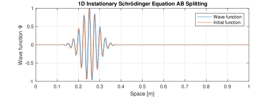
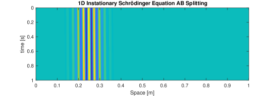
Figure 2: Simulations with the multiscale Schrödinger equation with AB-splitting method.

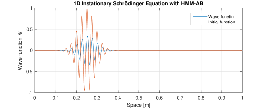
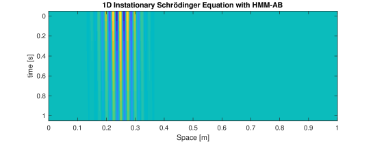
Figure 3: Simulations with the multiscale Schrödinger equation with HMM.

In the following, we have the error of the different schemes in Table 1.

Numerical method	Numerical error	M	$\tilde{M}$
AB Splitting	$6.081976027577089e-15$	$1$
AB Splitting	$6.081976027555089e-15$	$10$
AB Splitting	$6.081976027555089e-15$	$100$
ABA Splitting	$5.918971525959246e-15$	$1$
ABA Splitting	$5.918971525959246e-15$	$10$
ABA Splitting	$5.918971525959246e-15$	$100$
HMM-AB	$6.081976027555089e-15$	$1$	$1$
HMM-AB	$4.404021547293822e-12$	$10$	$5$
HMM-AB	Takes too long time	$100$	$50$
Extra-AB	$6.081976027555089e-15$	$1$	$1$
Extra-AB	$5.143436597696588e-15$	$10$	$5$
Extra-AB	$5.018633361834493e-15$	$100$	$50$
HigherExtra-AB	$6.081976027555089e-15$	$1$	$1$
HigherExtra-AB	$7.057484576752767e-15$	$10$	$5$
HigherExtra-AB	$9.995071997473121e-15$	$100$	$50$

Table 1: The numerical errors of the multiscale methods.

Further, we present the computational time of the different methods in Table 2:

Numerical Method	Computational Time in sec	Time-step
FD-Scheme	$4.691497$	$0.0008$
FD-Scheme	$8.785431$	$0.0004$
FD-Scheme	$18.329370$	$0.0002$
AB-Splitting	$4.560601$	$0.0008$
AB-Splitting	$9.263053$	$0.0004$
AB-Splitting	$18.514509$	$0.0002$
ABA-Splitting	$6.657831$	$0.0008$
ABA-Splitting	$13.508871$	$0.0004$
ABA-Splitting	$27.015384$	$0.0002$
BAB-Splitting	$6.731909$	$0.0008$
BAB-Splitting	$13.424463$	$0.0004$
BAB-Splitting	$28.469047$	$0.0002$
Extra-AB	$5.464744$	$0.0008$
Extra-AB	$10.982060$	$0.0004$
Extra-AB	$23.133747$	$0.0002$
HigherExtra-AB	$7.731819$	$0.0008$
HigherExtra-AB	$16.434144$	$0.0004$
HigherExtra-AB	$32.633806$	$0.0002$

Table 2: The computational time of the different methods.

Remark 9

Based on the separation of the macroscopic and microscopic operator, we can apply much more adapted time-steps. Further, we save more computational time to reduce the large amount of microscopic time-steps with extrapolation methods. The best results are obtained with the extrapolated AB splitting method, while we separate the operators and need only a smaller number of microscopic time-steps. Based on higher extrapolation schemes with ABA-splitting approaches, we could also improve the accuracy.

5 Conclusion

We presented a novel multiscale method, which is based on extrapolation methods and operator splitting approaches. Based on the separation of the microscopic and macroscopic operator, we could reduce the computational time. Further, we applied sufficient microscopic time-steps and extrapolate to the macroscopic time-step, which also reduce the computational amount. Based on the reduced numbers of finer time-steps, we could achieve faster numerical results with the same accurate results as for the standard AB-splitting scheme. Such novel schemes allow to flexiblise the standard operator splitting methods and modify such schemes to multiscale methods In future, we will test the new splitting approaches to higher dimensional Schrödinger equations and present the numerical analysis of the different schemes.

References

- [1] C. Brezinski and M. Redivo-Zaglia. Extrapolation methods. Applied Numerical Mathematics, 15(2): 123-131, 1994.
- [2] J.C. Butcher. Numerical methods for ordinary differential equations. 2nd edition, John Wiley & Sons, Inc. Hoboken, New Jersey, USA, 2008.
- [3] W. E., B. Engquist, X. Li, W. Ren, and E. Vanden-Eijnden. Heterogeneous Multiscale Methods: A Review. Communications in Computational Physics, 2(3), 367-450, 2007.
- [4] I. Farago and J. Geiser. Iterative Operator-Splitting methods for Linear Problems. International Journal of Computational Science and Engineering, 3(4), 255-263, 2007.
- [5] J. Geiser. Decomposition Methods for Partial Differential Equations: Theory and Applications in Multiphysics Problems. Numerical Analysis and Scientific Computing Series, Taylor & Francis Group, Boca Raton, London, New York, 2009.
- [6] J. Geiser. Iterative Splitting Methods for Differential Equations. Chapman & Hall/CRC Numerical Analysis and Scientific Computing Series, edited by Magoules and Lai, 2011.
- [7] J. Geiser. Multicomponent and Multiscale Systems: Theory, Methods, and Applications in Engineering. Springer, Cham, Heidelberg, New York, Dordrecht, London, 2016.
- [8] J. Geiser. Iterative splitting method as almost asymptotic symplectic integrator for stochastic nonlinear Schrödinger equation. AIP Conference Proceedings 1863, 560005, 2017.
- [9] J. Geiser. Multiscale Modelling and Splitting Approaches for Fluids composed of Coulomb-interacting Particles. Special-Issue: Problems with Multiple Time-scales Mathematical, Journal: Mathematical and Computer Modelling of Dynamical Systems, edited by J.Geiser, Taylor and Francis, Abingdon, UK, accepted January 2018.
- [10] D.J. Griffiths. Introduction to Quantum Mechanics. 2nd edn, Prentice Hall, Upper Saddle River, NJ, 2004.
- [11] E. Hairer and G. Wanner. Solving Ordinary Differential Equations II. SCM, Springer-Verlag, Berlin, Heidelberg, New York, No. 14, 1996.
- [12] I.G. Kevrekidis and G. Samaey. Equation-free multiscale computation: Algorithms and applications. Annual Review in Physical Chemistry 60:321–344, 2009.
- [13] P. Singh. High accuracy computational methods for the semiclassical Schrödinger equation. PhD Thesis, King fs College DAMTP, Centre for Mathematical Sciences, University of Cambridge, 2016.
- [14] G. Strang. On the construction and comparison of difference schemes. SIAM J. Numer. Anal., 5, 506-517, 1968.
- [15] L.A. Takhtajan. Quantum mechanics for mathematicians. Graduate Studies in Mathematics 95, Amer. Math. Soc., Providence, Rhode Island, 2008.
- [16] H.F. Trotter. On the product of semi-groups of operators. Proceedings of the American Mathematical Society, 10(4), 545-551, 1959.