To Trust Or Not To Trust A Classifier
Abstract
Knowing when a classifier’s prediction can be trusted is useful in many applications and critical for safely using AI. While the bulk of the effort in machine learning research has been towards improving classifier performance, understanding when a classifier’s predictions should and should not be trusted has received far less attention. The standard approach is to use the classifier’s discriminant or confidence score; however, we show there exists an alternative that is more effective in many situations. We propose a new score, called the trust score, which measures the agreement between the classifier and a modified nearest-neighbor classifier on the testing example. We show empirically that high (low) trust scores produce surprisingly high precision at identifying correctly (incorrectly) classified examples, consistently outperforming the classifier’s confidence score as well as many other baselines. Further, under some mild distributional assumptions, we show that if the trust score for an example is high (low), the classifier will likely agree (disagree) with the Bayes-optimal classifier. Our guarantees consist of non-asymptotic rates of statistical consistency under various nonparametric settings and build on recent developments in topological data analysis.
1 Introduction
Machine learning (ML) is a powerful and widely-used tool for making potentially important decisions, from product recommendations to medical diagnosis. However, despite ML’s impressive performance, it makes mistakes, with some more costly than others. As such, ML trust and safety is an important theme Varshney and Alemzadeh (2017); Lee and See (2004); Amodei et al. (2016). While improving overall accuracy is an important goal that the bulk of the effort in ML community has been focused on, it may not be enough: we need to also better understand the strengths and limitations of ML techniques.
This work focuses on one such challenge: knowing whether a classifier’s prediction for a test example can be trusted or not. Such trust scores have practical applications. They can be directly shown to users to help them gauge whether they should trust the AI system. This is crucial when a model’s prediction influences important decisions such as a medical diagnosis, but can also be helpful even in low-stakes scenarios such as movie recommendations. Trust scores can be used to override the classifier and send the decision to a human operator, or to prioritize decisions that human operators should be making. Trust scores are also useful for monitoring classifiers to detect distribution shifts that may mean the classifier is no longer as useful as it was when deployed. ††footnotetext: An open-source implementation of Trust Scores can be found here: https://github.com/google/TrustScore
A standard approach to deciding whether to trust a classifier’s decision is to use the classifiers’ own reported confidence or score, e.g. probabilities from the softmax layer of a neural network, distance to the separating hyperplane in support vector classification, mean class probabilities for the trees in a random forest. While using a model’s own implied confidences appears reasonable, it has been shown that the raw confidence values from a classifier are poorly calibrated (Guo et al., 2017; Kuleshov and Liang, 2015). Worse yet, even if the scores are calibrated, the ranking of the scores itself may not be reliable. In other words, a higher confidence score from the model does not necessarily imply higher probability that the classifier is correct, as shown in Provost et al. (1998); Goodfellow et al. (2014); Nguyen et al. (2015). A classifier may simply not be the best judge of its own trustworthiness.
In this paper, we use a set of labeled examples (e.g. training data or validation data) to help determine a classifier’s trustworthiness for a particular testing example. First, we propose a simple procedure that reduces the training data to a high density set for each class. Then we define the trust score—the ratio between the distance from the testing sample to the nearest class different from the predicted class and the distance to the predicted class—to determine whether to trust that classifier prediction.
Theoretically, we show that high/low trust scores correspond to high probability of agreement/disagreement with the Bayes-optimal classifier. We show finite-sample estimation rates when the data is full-dimension and supported on or near a low-dimensional manifold. Interestingly, we attain bounds that depend only on the lower manifold dimension and independent of the ambient dimension without any changes to the procedure or knowledge of the manifold. To our knowledge, these results are new and may be of independent interest.
Experimentally, we found that the trust score better identifies correctly-classified points for low and medium-dimension feature spaces than the model itself. However, high-dimensional feature spaces were more challenging, and we demonstrate that the trust score’s utility depends on the vector space used to compute the trust score differences.
2 Related Work
One related line of work is that of confidence calibration, which transforms classifier outputs into values that can be interpreted as probabilities, e.g. Platt (1999); Zadrozny and Elkan (2002); Niculescu-Mizil and Caruana (2005); Guo et al. (2017). In recent work, Kuleshov and Liang (2015) explore the structured prediction setting, and Lakshminarayanan et al. (2017) obtain confidence estimates by using ensembles of networks. These calibration techniques typically only use the the model’s reported score (and the softmax layer in the case of a neural network) for calibration, which notably preserves the rankings of the classifier scores. Similarly, Hendrycks and Gimpel (2016) considered using the softmax probabilities for the related problem of identifying misclassifications and mislabeled points.
Recent work explored estimating uncertainty for Bayesian neural networks and returning a distribution over the outputs (Gal and Ghahramani, 2016; Kendall and Gal, 2017). The proposed trust score does not change the network structure (nor does it assume any structure) and gives a single score, rather than a distribution over outputs as the representation of uncertainty.
The problem of classification with a reject option or learning with abstention Bartlett and Wegkamp (2008); Yuan and Wegkamp (2010); Cortes et al. (2016b); Grandvalet et al. (2009); Cortes et al. (2016a); Herbei and Wegkamp (2006); Cortes et al. (2017) is a highly related framework where the classifier is allowed to abstain from making a prediction at a certain cost. Typically such methods jointly learn the classifier and the rejection function. Note that the interplay between classification rate and reject rate is studied in many various forms e.g. (Chow, 1970; Dubuisson and Masson, 1993; Fumera et al., 2000; Santos-Pereira and Pires, 2005; Tortorella, 2000; Fumera and Roli, 2002; Landgrebe et al., 2006; El-Yaniv and Wiener, 2010; Wiener and El-Yaniv, 2011; Tax and Duin, 2008). Our paper assumes an already trained and possibly black-box classifier and learns the confidence scores separately, but we do not explicitly learn the appropriate rejection thresholds.
Whether to trust a classifier also arises in the setting where one has access to a sequence of classifiers, but there is some cost to evaluating each classifier, and the goal is to decide after evaluating each classifier in the sequence if one should trust the current classifier decision enough to stop, rather than evaluating more classifiers in the sequence (e.g. Wang et al. (2015); Parrish et al. (2013); Fan et al. (2002)). Those confidence decisions are usually based on whether the current classifier score will match the classification of the full sequence.
Experimentally we find that the vector space used to compute the distances in the trust score matters, and that computing trust scores on more-processed layers of a deep model generally works better. This observation is similar to the work of Papernot and McDaniel Papernot and McDaniel (2018), who use -NN regression on the intermediate representations of the network which they showed enhances robustness to adversarial attacks and leads to better calibrated uncertainty estimations.
Our work builds on recent results in topological data analysis. Our method to filter low-density points estimates a particular density level-set given a parameter , which aims at finding the level-set that contains fraction of the probability mass. Level-set estimation has a long history Hartigan (1975); Ester et al. (1996); Tsybakov et al. (1997); Singh et al. (2009); Rigollet et al. (2009); Jiang (2017a). However such works assume knowledge of the density level, which is difficult to determine in practice. We provide rates for Algorithm 1 in estimating the appropriate level-set corresponding to without knowledge of the level. The proxy offers a more intuitive parameter compared to the density value, is used for level-set estimation. Our analysis is also done under various settings including when the data lies near a lower dimensional manifold and we provide rates that depend only on the lower dimension.
3 Algorithm: The Trust Score
Our approach proceeds in two steps outlined in Algorithm 1 and 2. We first pre-process the training data, as described in Algorithm 1, to find the -high-density-set of each class, which is defined as the training samples within that class after filtering out -fraction of the samples with lowest density (which may be outliers):
Definition 1 (-high-density-set).
Let and be a continuous density function with compact support . Then define , the -high-density-set of , to be the -level set of , defined as where .
In order to approximate the -high-density-set, Algorithm 1 filters the -fraction of the sample points with lowest empirical density, based on -nearest neighbors. This data filtering step is independent of the given classifier .
Then, the second step: given a testing sample, we define its trust score to be the ratio between the distance from the testing sample to the -high-density-set of the nearest class different from the predicted class, and the distance from the test sample to the -high-density-set of the class predicted by , as detailed in Algorithm 2. The intuition is that if the classifier predicts a label that is considerably farther than the closest label, then this is a warning that the classifier may be making a mistake.
Our procedure can thus be viewed as a comparison to a modified nearest-neighbor classifier, where the modification lies in the initial filtering of points not in the -high-density-set for each class.
Remark 1.
The distances can be computed with respect to any representation of the data. For example, the raw inputs, an unsupervised embedding of the space, or the activations of the intermediate representations of the classifier. Moreover, the nearest-neighbor distance can be replaced by other distance measures, such as -nearest neighbors or distance to a centroid.
The method has two hyperparameters: (the number of neighbors, such as in -NN) and (fraction of data to filter) to compute the empirical densities. We show in theory that can lie in a wide range and still give us the desired consistency guarantees. Throughout our experiments, we fix , and use cross-validation to select as it is data-dependent.
Remark 2.
We observed that the procedure was not very sensitive to the choice of and . As will be shown in the experimental section, for efficiency on larger datasets, we skipped the initial filtering step of Algorithm 1 (leading to a hyperparameter-free procedure) and obtained reasonable results. This initial filtering step can also be replaced by other strategies. One such example is filtering examples whose labels have high disagreement amongst its neighbors, which is implemented in the open-source code release but not experimented with here.
4 Theoretical Analysis
In this section, we provide theoretical guarantees for Algorithms 1 and 2. Due to space constraints, all the proofs are deferred to the Appendix. To simplify the main text, we state our results treating , the confidence level, as a constant. The dependence on in the rates is made explicit in the Appendix.
We show that Algorithm 1 is a statistically consistent estimator of the -high-density-level set with finite-sample estimation rates. We analyze Algorithm 1 in three different settings: when the data lies on (i) a full-dimensional ; (ii) an unknown lower dimensional submanifold embedded in ; and (iii) an unknown lower dimensional submanifold with full-dimensional noise.
For setting (i), where the data lies in , the estimation rate has a dependence on the dimension , which may be unattractive in high-dimensional situations: this is known as the curse of dimensionality, suffered by density-based procedures in general. However, when the data has low intrinsic dimension in (ii), it turns out that, remarkably, without any changes to the procedure, the estimation rate depends on the lower dimension and is independent of the ambient dimension . However, in realistic situations, the data may not lie exactly on a lower-dimensional manifold, but near one. This reflects the setting of (iii), where the data essentially lies on a manifold but has general full-dimensional noise so the data is overall full-dimensional. Interestingly, we show that we still obtain estimation rates depending only on the manifold dimension and independent of the ambient dimension; moreover, we do not require knowledge of the manifold nor its dimension to attain these rates.
We then analyze Algorithm 2, and establish the culminating result of Theorem 4: for labeled data distributions with well-behaved class margins, when the trust score is large, the classifier likely agrees with the Bayes-optimal classifier, and when the trust score is small, the classifier likely disagrees with the Bayes-optimal classifier. If it turns out that even the Bayes-optimal classifier has high-error in a certain region, then any classifier will have difficulties in that region. Thus, Theorem 4 does not guarantee that the trust score can predict misclassification, but rather that it can predict when the classifier is making an unreasonable decision.
4.1 Analysis of Algorithm 1
We require the following regularity assumptions on the boundaries of , which are standard in analyses of level-set estimation Singh et al. (2009). Assumption 1.1 ensures that the density around has both smoothness and curvature. The upper bound gives smoothness, which is important to ensure that our density estimators are accurate for our analysis (we only require this smoothness near the boundaries and not globally). The lower bound ensures curvature: this ensures that is salient enough to be estimated. Assumption 1.2 ensures that does not get arbitrarily thin anywhere.
Assumption 1 (-high-density-set regularity).
Let . There exists s.t.
-
1.
for all .
-
2.
For all and , we have .
where denotes the boundary of a set , , and .
Our statistical guarantees are under the Hausdorff metric, which ensures a uniform guarantee over our estimator: it is a stronger notion of consistency than other common metrics Rigollet et al. (2009); Rinaldo and Wasserman (2010).
Definition 2 (Hausdorff distance).
.
We now give the following result for Algorithm 1. It says that as long as our density function satisfies the regularity assumptions stated earlier, and the parameter lies within a certain range, then we can bound the Hausdorff distance between what Algorithm 1 recovers and , the true -high-density set, from an i.i.d. sample drawn from of size . Then, as goes to , and grows as a function of , the quantity goes to .
Theorem 1 (Algorithm 1 guarantees).
Let and suppose that is continuous and has compact support and satisfies Assumption 1. There exists constants depending on and such that the following holds with probability at least . Suppose that satisfies . Then we have
Remark 3.
The condition on can be simplified by ignoring log factors: , which is a wide range. Setting to its allowed upper bound, we obtain our consistency guarantee of
The first term is due to the error from estimating the appropriate level given (i.e. identifying the level ) and the second term corresponds to the error for recovering the level set given knowledge of the level. The latter term matches the lower bound for level-set estimation up to log factors Tsybakov et al. (1997).
4.2 Analysis of Algorithm 1 on Manifolds
One of the disadvantages of Theorem 1 is that the estimation errors have a dependence on , the dimension of the data, which may be highly undesirable in high-dimensional settings. We next improve these rates when the data has a lower intrinsic dimension. Interestingly, we are able to show rates that depend only on the intrinsic dimension of the data, without explicit knowledge of that dimension nor any changes to the procedure. As common to related work in the manifold setting, we make the following regularity assumptions which are standard among works in manifold learning (e.g. (Niyogi et al., 2008; Genovese et al., 2012; Balakrishnan et al., 2013)).
Assumption 2 (Manifold Regularity).
is a -dimensional smooth compact Riemannian manifold without boundary embedded in compact subset with bounded volume. has finite condition number , which controls the curvature and prevents self-intersection.
Theorem 2 (Manifold analogue of Theorem 1).
Remark 4.
Setting to its allowed upper bound, we obtain (ignoring log factors),
The first term can be compared to that of the previous result where is replaced with . The second term is the error for recovering the level set on manifolds, which matches recent rates Jiang (2017a).
4.3 Analysis of Algorithm 1 on Manifolds with Full Dimensional Noise
In realistic settings, the data may not lie exactly on a low-dimensional manifold, but near one. We next present a result where the data is distributed along a manifold with additional full-dimensional noise. We make mild assumptions on the noise distribution. Thus, in this situation, the data has intrinsic dimension equal to the ambient dimension. Interestingly, we are still able to show that the rates only depend on the dimension of the manifold and not the dimension of the entire data.
Theorem 3.
Let and . Suppose that distribution is a weighted mixture where is a distribution with continous density supported on a -dimensional manifold satisfying Assumption 2 and is a (noise) distribution with continuous density with compact support over with . Suppose also that there exists such that for all and (where ) satisfies Assumption 1 for density . Let be the output of Algorithm 1 on a sample of size drawn i.i.d. from . Then, there exists constants depending on , , , and such that the following holds with probability at least . Suppose that satisfies , where . Then we have
The above result is compelling because it shows why our methods can work, even in high-dimensions, despite the curse of dimensionality of non-parametric methods. In typical real-world data, even if the data lies in a high-dimensional space, there may be far fewer degrees of freedom. Thus, our theoretical results suggest that when this is true, then our methods will enjoy far better convergence rates – even when the data overall has full intrinsic dimension due to factors such as noise.
4.4 Analysis of Algorithm 2: the Trust Score
We now provide a guarantee about the trust score, making the same assumptions as in Theorem 3 for each of the label distributions. We additionally assume that the class distributions are well-behaved in the following sense: that high-density-regions for each of the classes satisfy the property that for any point , if the ratio of the distance to one class’s high-density-region to that of another is smaller by some margin , then it is more likely that ’s label corresponds to the former class.
Theorem 4.
Let . Let us have labeled data drawn from distribution , which is a joint distribution over where are the labels, , and is compact. Suppose for each , the conditional distribution for label satisfies the conditions of Theorem 3 for some manifold and noise level . Let be the density of the portion of the conditional distribution for label supported on . Define , where and let be the maximum Hausdorff error from estimating over each in Theorem 3. Assume that to ensure we have samples from each label.
Suppose also that for each , if then for . That is, if we are closer to than by a ratio of less than , then the point is more likely to be from class . Let be the Bayes-optimal classifier, defined by . Then the trust score of Algorithm 2 satisfies the following with high probability uniformly over all and all classifiers simultaneously for sufficiently large depending on :
5 Experiments
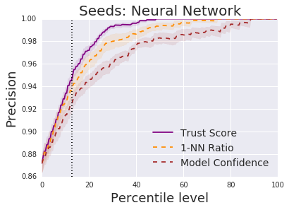
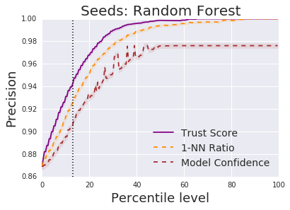
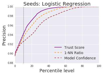
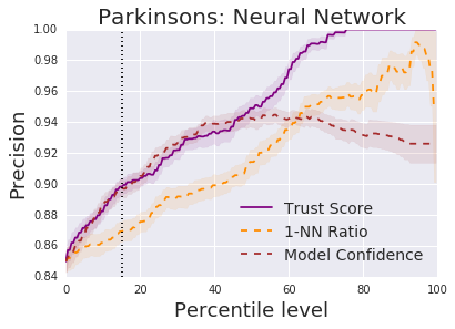
In this section, we empirically test whether trust scores can both detect examples that are incorrectly classified with high precision and be used as a signal to determine which examples are likely correctly classified. We perform this evaluation across (i) different datasets (Sections 5.1 and 5.3), (ii) different families of classifiers (neural network, random forest and logistic regression) (Section 5.1), (iii) classifiers with varying accuracy on the same task (Section 5.2) and (iv) different representations of the data e.g. input data or activations of various intermediate layers in neural network (Section 5.3).
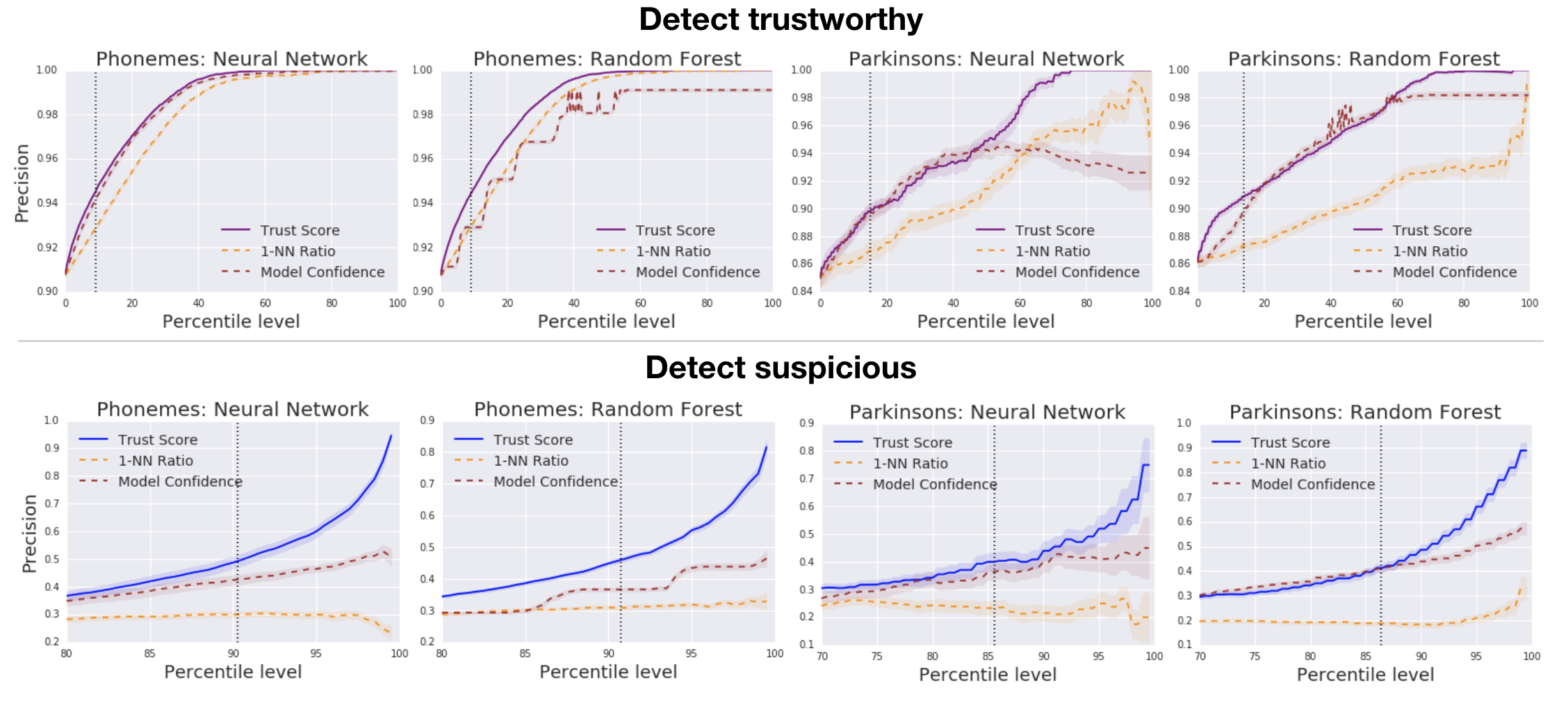
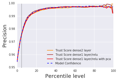
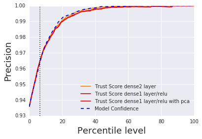
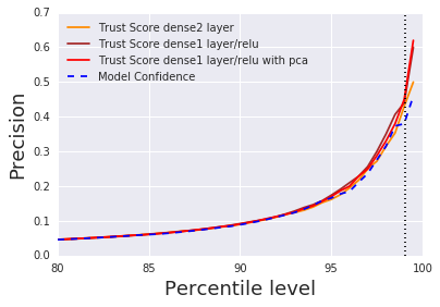
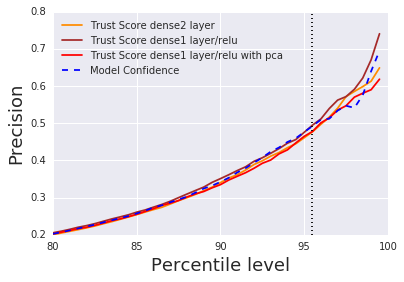
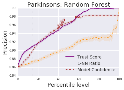
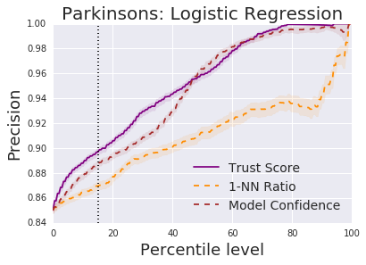
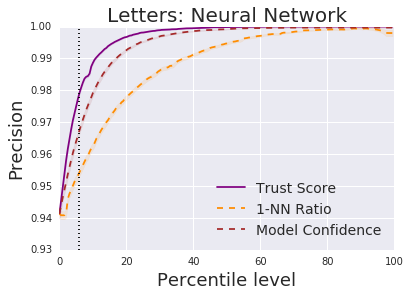
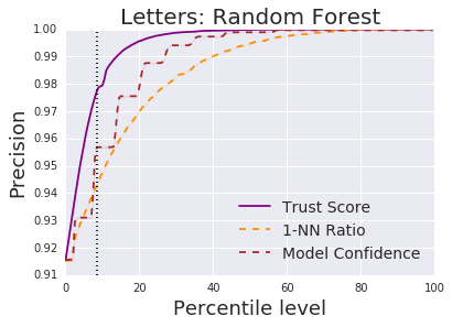
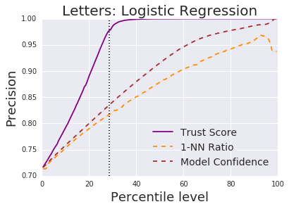
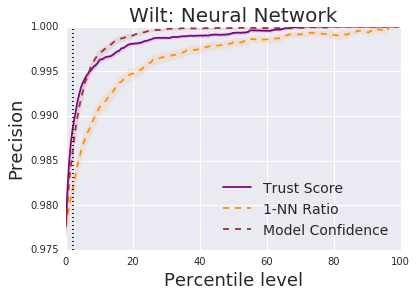
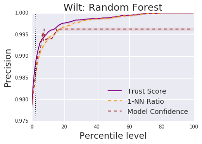
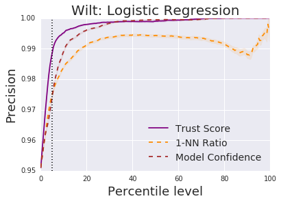
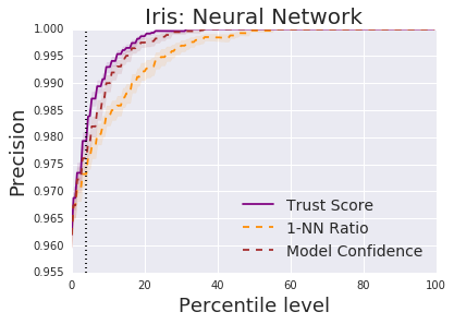
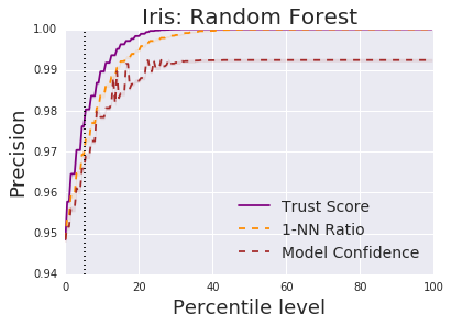
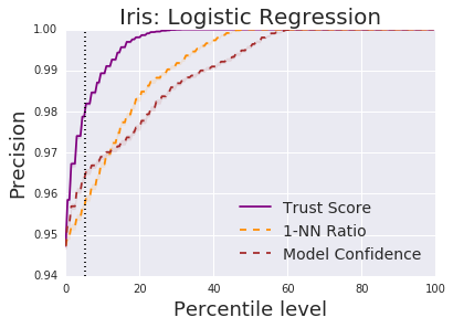
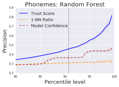
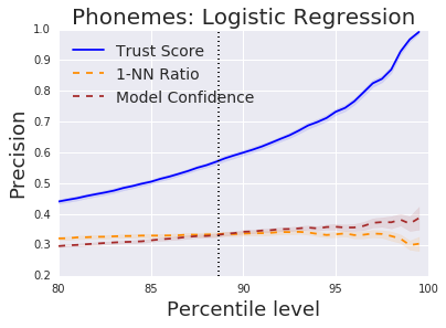
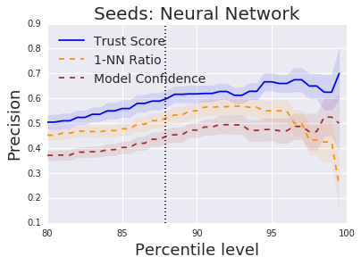
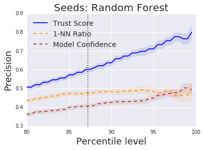
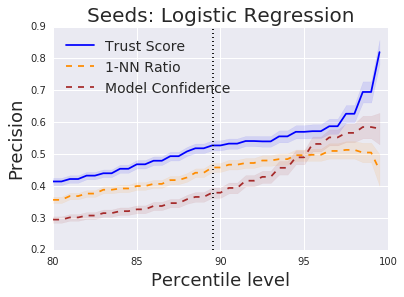
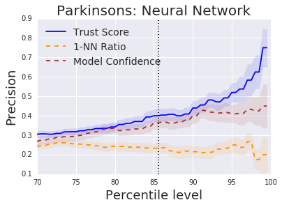
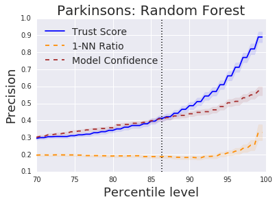
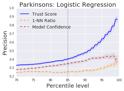
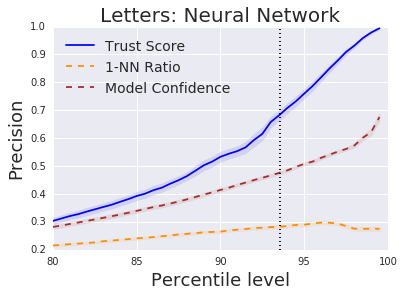
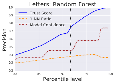
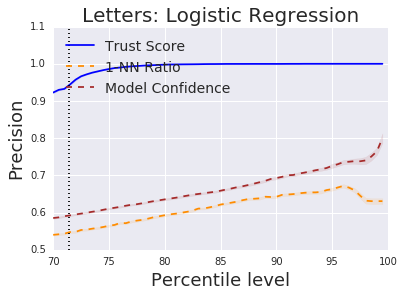
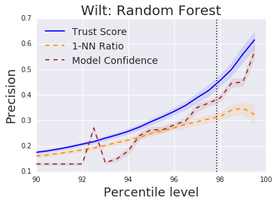
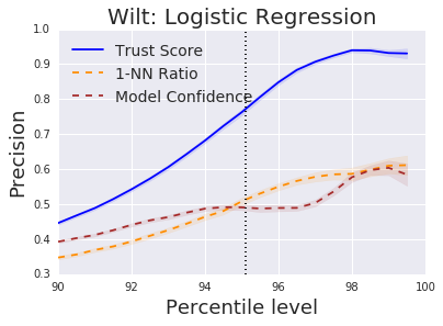
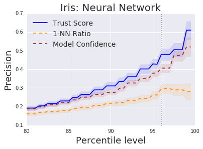
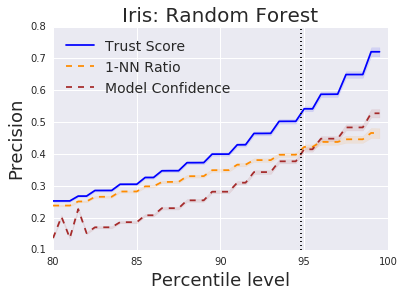
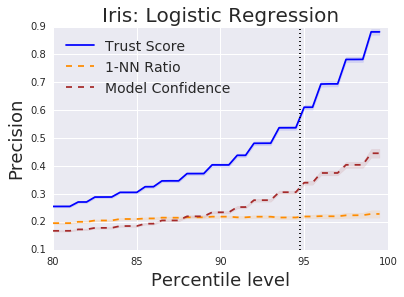
First, we test if testing examples with high trust score corresponds to examples in which the model is correct ("identifying trustworthy examples"). Each method produces a numeric score for each testing example. For each method, we bin the data points by percentile value of the score (i.e. 100 bins). Given a recall percentile level (i.e. the -axis on our plots), we take the performance of the classifier on the bins above the percentile level as the precision (i.e. the -axis). Then, we take the negative of each signal and test if low trust score corresponds to the model being wrong ("identifying suspicious examples"). Here the -axis is the misclassification rate and the -axis corresponds to decreasing trust score or model confidence.
In both cases, the higher the precision vs percentile curve, the better the method. The vertical black dotted lines in the plots represent the omniscient ideal. For identifying trustworthy examples it is the error rate of the classifier and for identifying suspicious examples" it is the accuracy rate.
The baseline we use in Section is the model’s own confidence score, which is similar to the approach of Hendrycks and Gimpel (2016). While calibrating the classifiers’ confidence scores (i.e. transforming them into probability estimates of correctness) is an important related work Guo et al. (2017); Platt (1999), such techniques typically do not change the rankings of the score, at least in the binary case. Since we evaluate the trust score on its precision at a given recall percentile level, we are interested in the relative ranking of the scores rather than their absolute values. Thus, we do not compare against calibration techniques. There are surprisingly few methods aimed at identifying correctly or incorrectly classified examples with precision at a recall percentile level as noted in Hendrycks and Gimpel (2016).
Choosing Hyperparameters: The two hyperparameters for the trust score are and . Throughout the experiments, we fix and choose using cross-validation over (negative) powers of on the training set. The metric for cross-validation was optimal performance on detecting suspicious examples at the percentile corresponding to the classifier’s accuracy. The bulk of the computational cost for the trust-score is in -nearest neighbor computations for training and -nearest neighbor searches for evaluation. To speed things up for the larger datasets MNIST, SVHN, CIFAR-10 and CIFAR-100, we skipped the initial filtering step of Algorithm 1 altogether and reduced the intermediate layers down to dimensions using PCA before being processed by the trust score which showed similar performance. We note that any approximation method (such as approximate instead of exact nearest neighbors) could have been used instead.
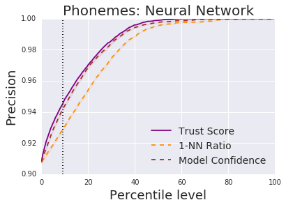
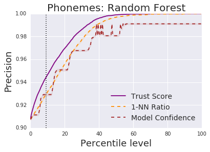
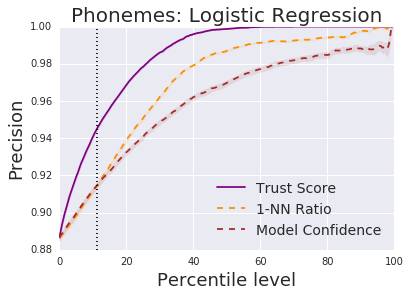
5.1 Performance on Benchmark UCI Datasets
In this section, we show performance on five benchmark UCI datasets Friedman et al. (2001), each for three kinds of classifiers (neural network, random forest and logistic regression). Due to space, we only show two data sets and two models in Figure 1. The rest can be found in the Appendix. For each method and dataset, we evaluated with multiple runs. For each run we took a random stratified split of the dataset into two halves. One portion was used for training the trust score and the other was used for evaluation and the standard error is shown in addition to the average precision across the runs at each percentile level. The results show that our method consistently has a higher precision vs percentile curve than the rest of the methods across the datasets and models. This suggests the trust score considerably improves upon known methods as a signal for identifying trustworthy and suspicious testing examples for low-dimensional data.
In addition to the model’s own confidence score, we try one additional baseline, which we call the nearest neighbor ratio (1-nn ratio). It is the ratio between the 1-nearest neighbor distance to the closest and second closest class, which can be viewed as an analogue to the trust score without knowledge of the classifier’s hard prediction.
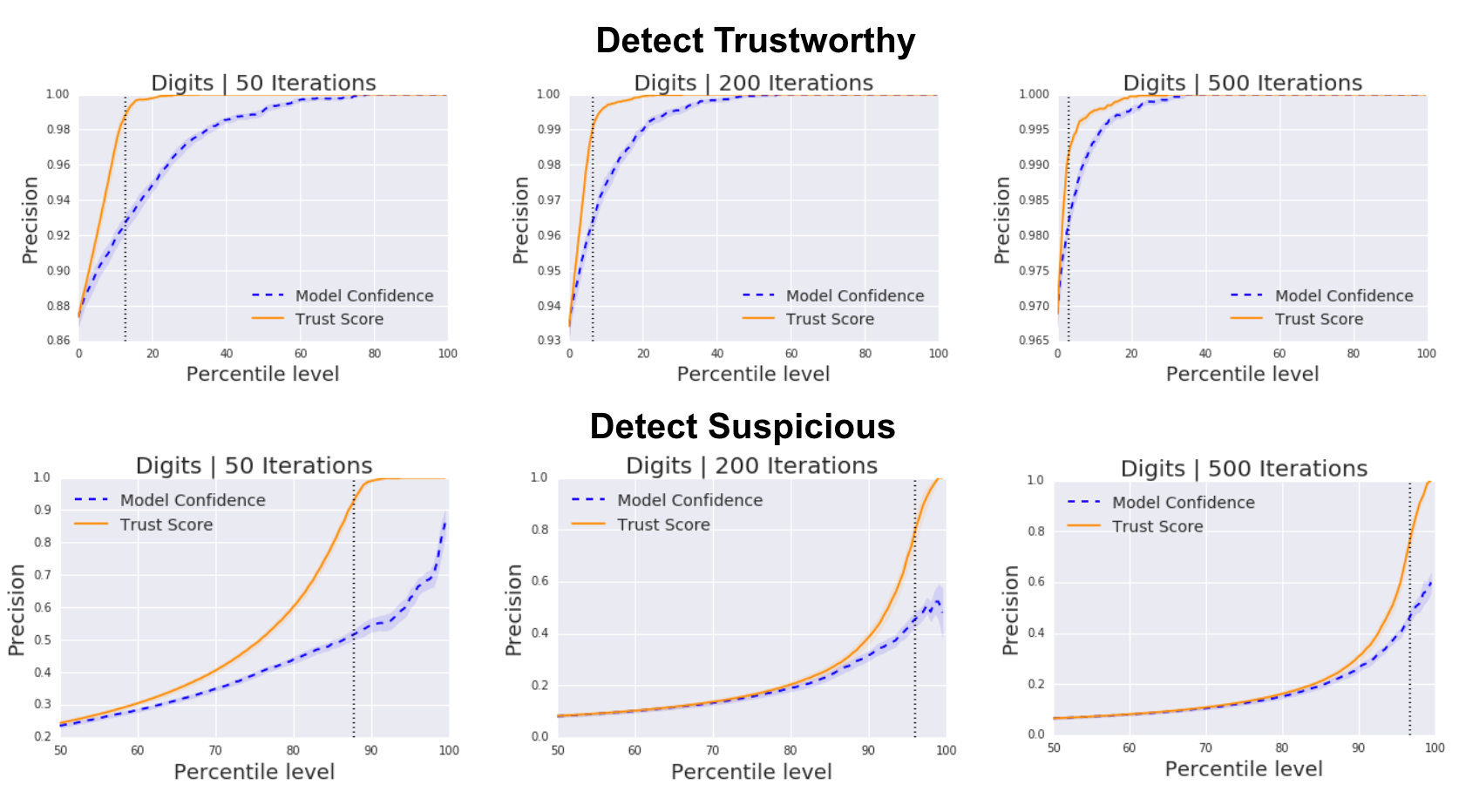
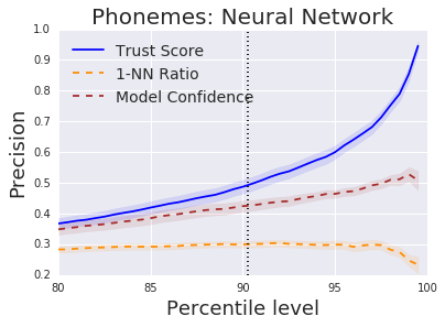
5.2 Performance as Model Accuracy Varies
In Figure 2, we show how the performance of trust score changes as the accuracy of the classifier changes (averaged over 20 runs for each condition). We observe that as the accuracy of the model increases, while the trust score still performs better than model confidence, the amount of improvement diminishes. This suggests that as the model improves, the information trust score can provide in addition to the model confidence decreases. However, as we show in Section 5.3, the trust score can still have added value even when the classifier is known to be of high performance on some benchmark larger-scale datasets.
5.3 Performance on MNIST, SVHN, CIFAR-10 and CIFAR-100 Datasets
The MNIST handwritten digit dataset LeCun (1998) consists of 60,000 2828-pixel training images and 10,000 testing images in 10 classes. The SVHN dataset Netzer et al. (2011) consists of 73,257 3232-pixel colour training images and 26,032 testing images and also has 10 classes. The CIFAR-10 and CIFAR-100 datasets Krizhevsky (2009) both consist of 60,000 3232-pixel colour images, with 50,000 training images and 10,000 test images. The CIFAR-10 and CIFAR-100 datasets are split evenly between 10 classes and 100 classes respectively.
We used a pretrained††https://github.com/geifmany/cifar-vgg VGG-16 Simonyan and Zisserman (2014) architecture with adaptation to the CIFAR datasets based on Liu and Deng (2015). The CIFAR-10 VGG-16 network achieves a test accuracy of 93.56% while the CIFAR-100 network achieves a test accuracy of 70.48%. We used pretrained, smaller CNNs for MNIST††https://github.com/EN10/KerasMNIST and SVHN††https://github.com/tohinz/SVHN-Classifier. The MNIST network achieves a test accuracy of 99.07% and the SVHN network achieves a test accuracy of 95.45%. All architectures were implemented in Keras Chollet et al. (2015).
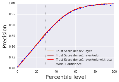
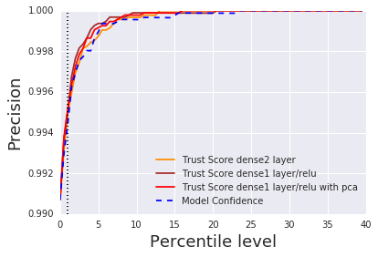
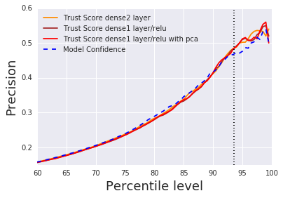
One simple generalization of our method is to use intermediate layers of a neural network as an input instead of the raw . Many prior work suggests that a neural network may learn different representations of at each layer. As input to the trust score, we tried using 1) the logit layer, 2) the preceding fully connected layer with ReLU activation, 3) this fully connected layer, which has 128 dimensions in the MNIST network and 512 dimensions in the other networks, reduced down to 20 dimensions from applying PCA.
The trust score results on various layers are shown in Figure 3. They suggest that for high dimensional datasets, the trust score may only provide little or no improvement over the model confidence at detecting trustworthy and suspicious examples. All plots were made using ; using cross-validation to select a different did not improve trust score performance. We also did not see much difference from using different layers.
Conclusion:
In this paper, we provide the trust score: a new, simple, and effective way to judge if one should trust the prediction from a classifier. The trust score provides information about the relative positions of the datapoints, which may be lost in common approaches such as the model confidence when the model is trained using SGD. We show high-probability non-asymptotic statistical guarantees that high (low) trust scores correspond to agreement (disagreement) with the Bayes-optimal classifier under various nonparametric settings, which build on recent results in topological data analysis. Our empirical results across many datasets, classifiers, and representations of the data show that our method consistently outperforms the classifier’s own reported confidence in identifying trustworthy and suspicious examples in low to mid dimensional datasets. The theoretical and empirical results suggest that this approach may have important practical implications in low to mid dimension settings.
References
- Amodei et al. (2016) Dario Amodei, Chris Olah, Jacob Steinhardt, Paul F Christiano, John Schulman, and Dan Mané. Concrete problems in AI safety. CoRR, abs/1606.06565, 2016. URL http://arxiv.org/abs/1606.06565.
- Balakrishnan et al. (2013) Sivaraman Balakrishnan, Srivatsan Narayanan, Alessandro Rinaldo, Aarti Singh, and Larry Wasserman. Cluster trees on manifolds. In Advances in Neural Information Processing Systems, pages 2679–2687, 2013.
- Bartlett and Wegkamp (2008) Peter L Bartlett and Marten H Wegkamp. Classification with a reject option using a hinge loss. Journal of Machine Learning Research, 9(Aug):1823–1840, 2008.
- Chaudhuri and Dasgupta (2010) Kamalika Chaudhuri and Sanjoy Dasgupta. Rates of convergence for the cluster tree. In Advances in Neural Information Processing Systems, pages 343–351, 2010.
- Chazal (2013) Frédéric Chazal. An upper bound for the volume of geodesic balls in submanifolds of Euclidean spaces. https://geometrica.saclay.inria.fr/team/Fred.Chazal/BallVolumeJan2013.pdf, 2013.
- Chollet et al. (2015) François Chollet et al. Keras. 2015.
- Chow (1970) C Chow. On optimum recognition error and reject tradeoff. IEEE Transactions on Information Theory, 16(1):41–46, 1970.
- Cortes et al. (2016a) Corinna Cortes, Giulia DeSalvo, and Mehryar Mohri. Boosting with abstention. In Advances in Neural Information Processing Systems, pages 1660–1668, 2016a.
- Cortes et al. (2016b) Corinna Cortes, Giulia DeSalvo, and Mehryar Mohri. Learning with rejection. In International Conference on Algorithmic Learning Theory, pages 67–82. Springer, 2016b.
- Cortes et al. (2017) Corinna Cortes, Giulia DeSalvo, Claudio Gentile, Mehryar Mohri, and Scott Yang. Online learning with abstention. arXiv preprint arXiv:1703.03478, 2017.
- Dasgupta and Kpotufe (2014) Sanjoy Dasgupta and Samory Kpotufe. Optimal rates for k-NN density and mode estimation. In Advances in Neural Information Processing Systems, pages 2555–2563, 2014.
- Devroye et al. (1994) Luc Devroye, Laszlo Gyorfi, Adam Krzyzak, and Gábor Lugosi. On the strong universal consistency of nearest neighbor regression function estimates. The Annals of Statistics, pages 1371–1385, 1994.
- Dubuisson and Masson (1993) Bernard Dubuisson and Mylene Masson. A statistical decision rule with incomplete knowledge about classes. Pattern Recognition, 26(1):155–165, 1993.
- El-Yaniv and Wiener (2010) Ran El-Yaniv and Yair Wiener. On the foundations of noise-free selective classification. Journal of Machine Learning Research, 11(May):1605–1641, 2010.
- Ester et al. (1996) Martin Ester, Hans-Peter Kriegel, Jörg Sander, Xiaowei Xu, et al. A density-based algorithm for discovering clusters in large spatial databases with noise. In Kdd, pages 226–231, 1996.
- Fan et al. (2002) Wei Fan, Fang Chu, Haixun Wang, and Philip S. Yu. Pruning and dynamic scheduling of cost-sensitive ensembles. AAAI, 2002.
- Friedman et al. (2001) Jerome Friedman, Trevor Hastie, and Robert Tibshirani. The Elements of Statistical Learning. Springer, 2001.
- Fumera and Roli (2002) Giorgio Fumera and Fabio Roli. Support vector machines with embedded reject option. In Pattern Recognition with Support Vector Machines, pages 68–82. Springer, 2002.
- Fumera et al. (2000) Giorgio Fumera, Fabio Roli, and Giorgio Giacinto. Multiple reject thresholds for improving classification reliability. In Joint IAPR International Workshops on Statistical Techniques in Pattern Recognition (SPR) and Structural and Syntactic Pattern Recognition (SSPR), pages 863–871. Springer, 2000.
- Gal and Ghahramani (2016) Yarin Gal and Zoubin Ghahramani. Dropout as a Bayesian approximation: Representing model uncertainty in deep learning. In International Conference on Machine Learning, pages 1050–1059, 2016.
- Genovese et al. (2012) Christopher Genovese, Marco Perone-Pacifico, Isabella Verdinelli, and Larry Wasserman. Minimax manifold estimation. Journal of Machine Learning Research, 13(May):1263–1291, 2012.
- Goodfellow et al. (2014) Ian J Goodfellow, Jonathon Shlens, and Christian Szegedy. Explaining and harnessing adversarial examples. arXiv preprint arXiv:1412.6572, 2014.
- Grandvalet et al. (2009) Yves Grandvalet, Alain Rakotomamonjy, Joseph Keshet, and Stéphane Canu. Support vector machines with a reject option. In Advances in Neural Information Processing Systems, pages 537–544, 2009.
- Guo et al. (2017) Chuan Guo, Geoff Pleiss, Yu Sun, and Kilian Q Weinberger. On calibration of modern neural networks. arXiv preprint arXiv:1706.04599, 2017.
- Hartigan (1975) John A Hartigan. Clustering algorithms. 1975.
- Hendrycks and Gimpel (2016) Dan Hendrycks and Kevin Gimpel. A baseline for detecting misclassified and out-of-distribution examples in neural networks. arXiv preprint arXiv:1610.02136, 2016.
- Herbei and Wegkamp (2006) Radu Herbei and Marten H Wegkamp. Classification with reject option. Canadian Journal of Statistics, 34(4):709–721, 2006.
- Jiang (2017a) Heinrich Jiang. Density level set estimation on manifolds with DBSCAN. In International Conference on Machine Learning, pages 1684–1693, 2017a.
- Jiang (2017b) Heinrich Jiang. Uniform convergence rates for kernel density estimation. In International Conference on Machine Learning, pages 1694–1703, 2017b.
- Kendall and Gal (2017) Alex Kendall and Yarin Gal. What uncertainties do we need in Bayesian deep learning for computer vision? In Advances in Neural Information Processing Systems, pages 5580–5590, 2017.
- Krizhevsky (2009) Alex Krizhevsky. Learning multiple layers of features from tiny images. 2009.
- Kuleshov and Liang (2015) Volodymyr Kuleshov and Percy S Liang. Calibrated structured prediction. In Advances in Neural Information Processing Systems, pages 3474–3482, 2015.
- Lakshminarayanan et al. (2017) Balaji Lakshminarayanan, Alexander Pritzel, and Charles Blundell. Simple and scalable predictive uncertainty estimation using deep ensembles. In Advances in Neural Information Processing Systems, pages 6405–6416, 2017.
- Landgrebe et al. (2006) Thomas CW Landgrebe, David MJ Tax, Pavel Paclík, and Robert PW Duin. The interaction between classification and reject performance for distance-based reject-option classifiers. Pattern Recognition Letters, 27(8):908–917, 2006.
- LeCun (1998) Yann LeCun. The MNIST database of handwritten digits. http://yann. lecun. com/exdb/mnist/, 1998.
- Lee and See (2004) John D Lee and Katrina A See. Trust in automation: Designing for appropriate reliance. Human factors, 46(1):50–80, 2004.
- Liu and Deng (2015) Shuying Liu and Weihong Deng. Very deep convolutional neural network based image classification using small training sample size. 2015 3rd IAPR Asian Conference on Pattern Recognition (ACPR), pages 730–734, 2015.
- Netzer et al. (2011) Yuval Netzer, Tao Wang, Adam Coates, Alessandro Bissacco, Bo Wu, and Andrew Y Ng. Reading digits in natural images with unsupervised feature learning. 2011.
- Nguyen et al. (2015) Anh Nguyen, Jason Yosinski, and Jeff Clune. Deep neural networks are easily fooled: High confidence predictions for unrecognizable images. In Proceedings of the IEEE Conference on Computer Vision and Pattern Recognition, pages 427–436, 2015.
- Niculescu-Mizil and Caruana (2005) Alexandru Niculescu-Mizil and Rich Caruana. Predicting good probabilities with supervised learning. In Proceedings of the 22nd International Conference on Machine Learning, pages 625–632. ACM, 2005.
- Niyogi et al. (2008) Partha Niyogi, Stephen Smale, and Shmuel Weinberger. Finding the homology of submanifolds with high confidence from random samples. Discrete & Computational Geometry, 39(1-3):419–441, 2008.
- Papernot and McDaniel (2018) Nicolas Papernot and Patrick McDaniel. Deep k-nearest neighbors: Towards confident, interpretable and robust deep learning. arXiv preprint arXiv:1803.04765, 2018.
- Parrish et al. (2013) Nathan Parrish, Hyrum S. Anderson, Maya R. Gupta, and Dun Yu Hsaio. Classifying with confidence from incomplete information. Journal of Machine Learning Research, 14(December):3561–3589, 2013.
- Platt (1999) John Platt. Probabilistic outputs for support vector machines and comparisons to regularized likelihood methods. Advances in Large Margin Classifiers, 10(3):61–74, 1999.
- Provost et al. (1998) Foster J Provost, Tom Fawcett, and Ron Kohavi. The case against accuracy estimation for comparing induction algorithms. In ICML, volume 98, pages 445–453, 1998.
- Rigollet et al. (2009) Philippe Rigollet, Régis Vert, et al. Optimal rates for plug-in estimators of density level sets. Bernoulli, 15(4):1154–1178, 2009.
- Rinaldo and Wasserman (2010) Alessandro Rinaldo and Larry Wasserman. Generalized density clustering. The Annals of Statistics, 38(5):2678–2722, 2010.
- Santos-Pereira and Pires (2005) Carla M Santos-Pereira and Ana M Pires. On optimal reject rules and ROC curves. Pattern Recognition Letters, 26(7):943–952, 2005.
- Simonyan and Zisserman (2014) Karen Simonyan and Andrew Zisserman. Very deep convolutional networks for large-scale image recognition. arXiv preprint arXiv:1409.1556, 2014.
- Singh et al. (2009) Aarti Singh, Clayton Scott, Robert Nowak, et al. Adaptive Hausdorff estimation of density level sets. The Annals of Statistics, 37(5B):2760–2782, 2009.
- Tax and Duin (2008) David MJ Tax and Robert PW Duin. Growing a multi-class classifier with a reject option. Pattern Recognition Letters, 29(10):1565–1570, 2008.
- Tortorella (2000) Francesco Tortorella. An optimal reject rule for binary classifiers. In Joint IAPR International Workshops on Statistical Techniques in Pattern Recognition (SPR) and Structural and Syntactic Pattern Recognition (SSPR), pages 611–620. Springer, 2000.
- Tsybakov et al. (1997) Alexandre B Tsybakov et al. On nonparametric estimation of density level sets. The Annals of Statistics, 25(3):948–969, 1997.
- Varshney and Alemzadeh (2017) Kush R Varshney and Homa Alemzadeh. On the safety of machine learning: Cyber-physical systems, decision sciences, and data products. Big data, 5(3):246–255, 2017.
- Wang et al. (2015) Joseph Wang, Kirill Trapeznikov, and Venkatesh Saligrama. Efficient learning by directed acyclic graph for resource constrained prediction. Advances in Neural Information Processing Systems (NIPS), 2015.
- Wiener and El-Yaniv (2011) Yair Wiener and Ran El-Yaniv. Agnostic selective classification. In Advances in Neural Information Processing Systems, pages 1665–1673, 2011.
- Yuan and Wegkamp (2010) Ming Yuan and Marten Wegkamp. Classification methods with reject option based on convex risk minimization. Journal of Machine Learning Research, 11(Jan):111–130, 2010.
- Zadrozny and Elkan (2002) Bianca Zadrozny and Charles Elkan. Transforming classifier scores into accurate multiclass probability estimates. In Proceedings of the Eighth ACM SIGKDD International Conference on Knowledge Discovery and Data Mining, pages 694–699. ACM, 2002.
Appendix
Appendix A Supporting results for Theorem 1 Proof
We need the following result giving guarantees on the empirical balls.
Lemma 1 (Uniform convergence of balls (Chaudhuri and Dasgupta, 2010)).
Let be the distribution corresponding to and be the empirical distribution corresponding to the sample . Pick . Assume that . Then with probability at least , for every ball we have
where
Remark 5.
For the rest of the paper, many results are qualified to hold with probability at least . This is precisely the event in which Lemma 1 holds.
Remark 6.
If , then .
Definition 3.
Define the -NN radius of as
Definition 4 (k-NN Density Estimator).
where is the volume of a unit ball in .
We will use bounds on the -NN density estimator from Dasgupta and Kpotufe (2014), which are repeated here.
Define the following one-sided modulus of continuity which characterizes how much the density increases locally:
Lemma 2 (Lemma 3 of Dasgupta and Kpotufe (2014)).
Suppose that . Then with probability at least , the following holds for all and .
provided satisfies .
Analogously, define the following which characterizes how much the density decreases locally:
Lemma 3 (Lemma 4 of Dasgupta and Kpotufe (2014)).
Suppose that . Then with probability at least , the following holds for all and .
provided satisfies .
Appendix B Proof of Theorem 1
In this section, we assume the conditions of Theorem 1. We first show that , that is the density level corresponding to the -high-density-set, is smooth in .
Lemma 4.
There exists constants depending on such that the following holds for all such that
Proof.
We have
where the first equality holds by definition. Choosing sufficiently small such that Assumption 1 holds, we have
where the last inequality holds for some constant depending on and Vol is the volume w.r.t. to the Lebesgue measure in . It then follows that
and the result for the first part follows by taking and . Showing that can be done analogously and is omitted here. ∎
The next result gets a handle on the density level corresponding to returned by Algorithm 1.
Lemma 5.
Let . Let be the setting chosen by Algorithm 1. Define
Then, with probability at least , we have there exist constant depending on such that for sufficiently large depending on , we have
Proof.
Let . Then, we have that if , then . Thus, the probability that a sample point falls in is a Bernoulli random variable with probability . Hence, by Hoeffding’s inequality, we have that there exist constant such that
Then it follows that choosing we get
Similarly, choosing gives us
Next, define
where will be chosen later in order for . By Lemma 4, there exists depending on such that for (which holds for sufficiently large depending on by Lemma 1), we have . As such, it suffices to choose such that for all such that if then . This is because would contain , which we showed earlier contains at least fraction of the samples. Define such that We have by Assumption 1,
Then, there exists constant sufficiently large depending on such that if
then the conditions in Lemma 3 are satisfied for sufficiently large. Thus, we have for all with , then . Hence, .
We now do the same in the other direction. Define
where will be chosen such that . By Lemma 4, it suffices to show that if then . This direction follows a similar argument as the previous.
Thus, there exists a constant depending on such that for sufficiently large depending on , we have:
as desired. ∎
The next result bounds between two level sets of .
Lemma 6.
Let . There exists constant depending on such that the following holds with probability at least for sufficiently large depending on . Define
Then,
Proof.
To simplify notation, let us define the following:
By Lemma 5, there exists such that defining
then we have
It suffices to show that there exists a constant such that
We start by showing . To do this, show that for any satisfying satisfies , where will be chosen later. By a similar argument as in the proof of Lemma 5, we can choose for some constant and the desired result holds for sufficiently large. Similarly, there exists such that implies that . The result follows by taking . ∎
We are now ready to prove Theorem 5, a more general version of Theorem 1 which makes the dependence on explicit. Note that if , then .
Theorem 5.
Proof of Theorem 5.
Again, to simplify notation, let us define the following:
There are two directions to show for the Hausdorff distance result. That (i) is bounded, that is none of the high-density points recovered by Algorithm 1 are far from the true high-density region; and (ii) that is bounded, that Algorithm 1 recovers a good covering of the entire high-density region.
We first show (i). By Lemma 6, we have that there exists such that
contains . Thus,
where the second inequality holds by Assumption 1. Now for the other direction, we have by triangle inequality that
The first term can be bounded by using Assumption 1:
Now for the second term, we see that by Lemma 6, contains all of the sample points of . Thus, we have
By Assumption 1, for , and we have , where is the distribution corresponding to . Choosing gives us that by Lemma 1 that where is the distribution of and thus, we have
which is dominated by the error contributed by the other error and the result follows. ∎
Appendix C Supporting results for Theorem 2 Proof
In this section, we note that we will reuse some notation from the last section for the manifold case.
Lemma 7 (Manifold version of uniform convergence of empirical Euclidean balls (Lemma 7 of Balakrishnan et al. (2013))).
Let be the true distribution and be the empirical distribution w.r.t. sample . Let be a minimal fixed set such that each point in is at most distance from some point in . There exists a universal constant such that the following holds with probability at least . For all ,
where , is the empirical distribution, and .
Definition 5 (k-NN Density Estimator on Manifold).
Lemma 8 (Manifold version of upper bound Jiang (2017a)).
Define the following which charaterizes how much the density increases locally in :
Fix and and suppose that . Then there exists constant such that if
then the following holds with probability at least uniformly in and with :
provided satisfies .
Lemma 9 (Manifold version of lower bound Jiang (2017a)).
Define the following which charaterizes how much the density decreases locally in :
Fix and and suppose . Then there exists constant such that if
then with probability at least , the following holds uniformly for all and with :
provided satisfies .
Appendix D Proof of Theorem 2
The proof essentially follows the same structure as the full-dimensional case, with the primary difference in the density estimation bounds.
Lemma 10 (Manifold Version of Lemma 4).
There exists constants depending on such that the following holds for all such that
Proof.
The proof follows the same structure as the proof of Lemma 4, with the difference being the change in dimension, and is omitted here. ∎
Lemma 11 (Manifold Version of Lemma 5).
Let . Let be the setting chosen by Algorithm 1 after the binary search procedure. Define
Then, with probability at least , we have there exist constant depending on and such that for sufficiently large depending on and , we have
Proof.
The proof is essentially the same as that of Lemma 5. The only difference is that instead of applying the full-dimensional versions of the uniform -NN density estimate bounds (Lemma 2 and 3), we instead apply the manifold analogues (Lemma 8 and 9). Asides from constant factors, the major difference is in the allowable range for . In the full-dimensional case, we only need for the density estimation bounds to hold. However, here we require . ∎
Lemma 12 (Manifold Version of Lemma 5).
Let . There exists constant depending on and such that the following holds with probability at least for sufficiently large depending on and . Define
Then,
Proof.
Same comment as the proof for Lemma 11. ∎
Theorem 6.
[Extends Theorem 2] Let . Suppose that density function is continuous and supported on and Assumptions 1 and 2 hold. Suppose also that there exists such that for all . Then, there exists constants depending on such that the following holds with probability at least . Suppose that satisfies,
where . Then we have
Proof of Theorem 6.
Proof is the same as the full-dimensional case given the contributed Lemmas of this section and is omitted here. ∎
Appendix E Supporting Results for Theorem 3 Proof
Next, we need the following on the volume of the intersection of the Euclidean ball and ; this is required to get a handle on the true mass of the ball under in later arguments. The upper and lower bounds follow from Chazal (2013) and Lemma 5.3 of Niyogi et al. (2008). The proof can be found e.g. in Jiang (2017a).
Lemma 13 (Ball Volume).
If , and then
where is the volume of a unit ball in and is the volume w.r.t. the uniform measure on .
The next is a bound uniform convergence of balls:
Lemma 14 (Lemma 3 of Jiang (2017b)).
Let be the set of all balls in , is some distribution and is an empirical distribution. With probability at least , the following holds uniformly for every and :
where .
Appendix F Proof of Theorem 3
The first result says that within the manifold, the vast majority of the probability mass is attributed to the manifold distributions.
Lemma 15.
There exists depending on such that the following holds uniformly over and .
Proof.
Let and . We have
where the second inequality holds by Lemma 13 for sufficiently small. On the other hand, we have
Thus, we have there exists depending on , , and such that
as desired. ∎
We next show that points far away from do not get selected as high-density points by Algorithm 1.
Lemma 16.
There exists such that for any and sufficiently large depending on and , with probability at least , Algorithm 1 will not select any points outside of .
Proof.
By Assumption 1, we can choose sufficiently small so that for the density , . Then, at the -density level, we will be within the area where the regularity assumptions hold.
Next, by Hoeffding’s inequality, we have that there exist constant such that for :
Choosing , then it follows that with probability at least ,
satisfies . Next let
Let be the value of used by Algorithm 1. Now, it suffices to show that for sufficiently large depending on :
where is the empirical distribution. This is because Algorithm 1 filters out sample points whose -ball has less than sample points for its final value, which is the value which allows it to filter -fraction of the points.
By Lemma 15, it suffices to show that
where denote the fraction of samples drawn from which lie in w.r.t. our entire sample .
To bound the LHS, we have by Lemma 13
for some and is the modulus of continuity, that is (i.e. is uniformly continuous since it is continuous over a compact support, so as ).
Lemma 17 (Bounding density estimators w.r.t to entire sample vs w.r.t. samples on manifold).
For , define the following:
where the former is simply the -NN radius we’ve been using thus far and the latter is the -NN radius if we were to restrict the samples to only those that came from . Then likewise, define the analogous density estimators:
where again, the former is the usual -NN density estimator on manifolds. Then, there exists such that the following holds with high probability.
Proof.
By Lemma 14, there exists depending on and such that
and
where is the empirical distribution w.r.t. . Next, by Lemma 15, we have for some constant :
where the second last inequality holds for some constant by Lemma 7 and is some constant depending on and and . Then it follows that for some constant , we have
In the other direction, we trivially have , so
The result follows. ∎
Theorem 7.
[Extends Theorem 3] Let and . Suppose that distribution is a weighted mixture where is a distribution with continous density supported on a -dimensional manifold satisfying Assumption 2 and is a (noise) distribution with continuous density with compact support over with . Suppose also that there exists such that for all and (where ) satisfies Assumption 1 for density . Let be the output of Algorithm 1 on a sample of size drawn i.i.d. from . Then, there exists constants depending on , , , such that the following holds with probability at least . Suppose that satisfies
where . Then we have
Proof of Theorem 7.
The proof follows in a similar way as that of Theorem 6, except with the complexity of having added full-dimensional noise. We will only highlight the difference and provide a sketch of the proof here.
Lemma 16 and 17 give us a handle on the additional complexity when having separate noise distribution, compared to the earlier manifold setting of Theorem 2.
Lemma 16 guarantees that the points in lie in the inside of with margin. In particular, that means the noise points are filtered out by the algorithm and thus, we are reduced to reasoning about the -high-density-set of .
Then, Lemma 17 ensures that the -NN density estimator used for our analysis for the entire sample is actually quite close to the -NN density estimator with respect to within . In other words, we can use the -NN density estimator to estimate without knowing which samples of were in . Lemma 17 shows that the additional error in density estimation we obtain is , where the first inequality holds since and the latter holds from the conditions on . It turns out that this error term can be absorbed as a constant in the previous result of Theorem 6. ∎
Appendix G Proof of Theorem 4
Proof of Theorem 4.
For the first inequality, we have
where the first inequality holds by Theorem 3. This, along with the condition on and fromo the theorem statement, implies that
which implies that . For the second inequality, we have
where the first inequality holds by Theorem 3. Thus, if the condition of the theorem statement holds, then
for all , which implies that ∎
Appendix H Additional UCI Experiments
H.1 When to trust: Precision for correct predictions by percentile
H.2 When to not trust: Precision for misclassification predictions by percentile

H.3 High dimensional Datasets