Neutrino spectral split in the exact many-body formalism

Abstract

We consider the many-body system of neutrinos interacting with each other through neutral current weak force. Emerging many-body effects in such a system could play important roles in some astrophysical sites such as the core collapse supernovae. In the literature this many-body system is usually treated within the mean field approximation which is an effective one-body description based on omitting entangled neutrino states. In this paper, we consider the original many-body system in an effective two flavor mixing scenario under the single angle approximation and present a solution without using the mean field approximation. Our solution is formulated around a special class of many-body eigenstates which do not undergo any level crossings as the neutrino self-interaction rate decreases while the neutrinos radiate from the supernova. In particular, an initial state which consists of electron neutrinos and antineutrinos of an orthogonal flavor can be entirely decomposed in terms of those eigenstates. Assuming that the conditions are perfectly adiabatic so that the evolution of these eigenstates follow their variation with the interaction rate, we show that this initial state develops a spectral split at exactly the same energy predicted by the mean field formulation.

I Introduction

Neutrinos and photons are the most abundant particle species in the Universe Patrignani et al. (2016). In some astrophysical sites, neutrinos can reach sufficiently high densities to form a many-body system through mutual neutral current weak interactions. A prominent example of such a site is a core-collapse supernova explosion Burrows (1990); Kotake et al. (2006); Beacom (2010); Raffelt (1996): When the inert iron core of a massive star reaches the Chandrasekar mass limit, it collapses until a dense proto-neutron star forms at the center. The proto-neutron star is initially very hot because it carries a large amount of gravitational potential energy which is converted into heat during the collapse. In about $10$ s, it cools down by emitting of the order of $10^{58}$ neutrinos Colgate and White (1966); Woosley and Weaver (1986); Arnett et al. (1989). Since the neutrinos can easily pass through the outer layers of the star as the matter is pushed into the space by the shock wave, they can quickly carry the energy and the entropy away from the proto-neutron star. In fact, neutrino emission is a very fast and efficient cooling mechanism not only for a proto-neutron star, but also for black hole accretion disks Ruffert and Janka (1999); Popham et al. (1999); Narayan et al. (2001); Matteo et al. (2002); Chen and Beloborodov (2007); Malkus et al. (2012) and binary neutron star mergers Tian et al. (2017).

In this paper we explore the impact of many-body effects due to neutrino-neutrino interactions on the flavor evolution of neutrinos. We use the core-collapse supernova as the backdrop of our discussion on many-body effects. However, our intention is not to give a sophisticated analysis of neutrino flavor evolution in a realistic supernova environment, which has already been the subject of intense research for the past few decades due to the importance of neutrinos in several aspects of supernova physics(see, e.g., Fowler and Hoyle (1964); Barkat (1975); Epstein et al. (1988); Woosley et al. (1990, 1994, 2002)) and the possibility of observing them with the current detectors Totani et al. (1998); Katz and Spiering (2012); Scholberg (2012). The interested reader is referred to the excellent review articles in the literature Duan et al. (2010); Chakraborty et al. (2016).

Here our focus is on the many-body system formed by the neutrinos. In particular, we report on an exact solution of this many-body system in a simplified case and its comparison with the results obtained with the mean field approximation, which is used to treat the neutrino-neutrino interactions in an overwhelming majority of studies in the literature. The mean field approximation basically amounts to replacing the mutual interactions between individual particles by a description in which each particle interacts with an average field formed by all other particles. Such a treatment greatly simplifies an interacting many-body system by effectively reducing it to the study of independent particles moving in an “external” field. This field is determined from a simple self-consistency requirement: Since the mean field is collectively created by all the particles in the system, it should change in line with the evolution of individual particles. At the mathematical level, the mean field approximation works by blocking all entangled states in the Hilbert space because particles moving independently in a field cannot develop entanglements if they are not entangled in the first place. In practice, one starts with an unentangled one-body initial state, i.e., a state which consists of multiplication of one-body states. Then the evolution of the system is restricted to such states at later times. For a system consisting of $n$ particles, each of which can occupy $k$ different states, this amounts to replacing the original $k^{n}$ dimensional Hilbert space with $n$ individual $k$-dimensional Hilbert spaces.

The mean field approximation was applied to self-interacting neutrinos quite early on Samuel (1993); Raffelt et al. (1993); Sigl and Raffelt (1993); McKellar and Thomson (1994) and widely adopted in subsequent studies. It is also extensively used in various areas such as nuclear physics, condensed matter physics, and the physics of cold atom systems. Unlike the case for neutrinos, in those other fields one has the advantage of experimental access to the system under consideration. In particular, it is usually possible to measure the fluctuations of various quantities around their mean field values in order to assess the accuracy of the approximation. Although the general consensus is that the mean field approximation becomes more and more accurate with an increasing number of particles, there are some cases which do not agree with this simple expectation Gertjerenken and Weiss (2013). In fact the latter situations are usually sought after and actively studied by theorists Sørensen et al. (2001); Pezzé and Smerzi (2009) and experimentalists Estève et al. (2008) in cold atom systems in connection to such applications as cryptography and quantum computing. Those studies intentionally create conditions under which an initially unentangled system develops into a macroscopically entangled state through time evolution and, in doing so, significantly deviates from its mean field description.

In the context of neutrino astrophysics, one is naturally interested in the opposite question, i.e., if the mean field approximation provides an accurate description of self-interacting neutrinos. References Friedland and Lunardini (2003a); Bell et al. (2003) were the first papers to tackle this difficult question. Reference Friedland and Lunardini (2003a) was concerned with the microphysics and worked with small neutrino wave packages which undergo distinct scatterings from one another. The authors were interested in whether the entanglement can build up on the system which starts from a one-body state. In particular, they considered two intersecting beams of neutrinos, each of which consisted only of a particular flavor. Using a physically very transparent argument, they showed that the buildup of entangled states occurs at the timescale of an incoherent effect which is much longer than the timescale of a coherent effect relevant for self-interacting neutrinos. Therefore Ref. Friedland and Lunardini (2003a) concluded that the mean field picture provides an accurate description of the problem. Reference Bell et al. (2003) used a different picture in which neutrinos are represented by plane waves in a box so that they all interact with each other at the same time. The authors approached the problem numerically by simulating the exact many-body behavior of $14$ neutrinos and comparing it with the mean field prediction. In particular if the vacuum oscillations are ignored, which was the case in both Refs. Friedland and Lunardini (2003a) and Bell et al. (2003), then the mean field picture predicts that no flavor evolution would occur for a one-body initial state in which all neutrinos occupy flavor eigenstates. However, Ref. Bell et al. (2003) has found some flavor conversion for such an initial state in the exact many-body picture which indicated a possible breakdown of the mean field approximation. This apparent contradiction was resolved in a later study Friedland and Lunardini (2003b) which established the following two results: (1) As far as the coherent effects are concerned, the study of the problem is independent of the size of the neutrino wave packages, so the two descriptions of the problem in Refs. Friedland and Lunardini (2003a); Bell et al. (2003) are equivalent. (2) The time required for the flavor conversion observed in Ref. Bell et al. (2003) scales as expected from an incoherent effect with an increasing number of particles; i.e., it develops more slowly until it becomes irrelevant in comparison to the much faster coherent effects.

Here, our treatment of the exact many-body effects is, in some ways, similar to that of Ref. Bell et al. (2003): We use the plane wave picture, and we compare the exact many-body behavior of the system with the mean field prediction. However, there are important differences between our work and Refs. Friedland and Lunardini (2003a); Bell et al. (2003); Friedland and Lunardini (2003b). First of all, our formalism includes the vacuum oscillations which were ignored in those studies. This allows us to obtain a spectral split in the exact many-body formalism for the first time. Spectral splits (or swaps) are a particular kind of emergent behavior in which neutrinos of different flavors totally or partially exchange their energy spectra Duan et al. (2006, 2010). Since they are caused by an interplay between the one-particle terms (vacuum oscillations) and two-particle terms (self-interactions), one needs to incorporate both effects in the calculations in order to unfold such a behavior Raffelt and Smirnov (2007a, b); Pehlivan et al. (2011); Raffelt (2011); Galais and Volpe (2011). For this reason, spectral splits are so far observed only in the mean field calculations. Another difference between our work and the previous studies is that we use a semianalytical technique which allows us to numerically work with as many as $10^{8}$ neutrinos. Our technique is based on the algebraic Bethe ansatz formalism Bethe (1931); Richardson (1963); Gaudin (1976, 1983); Dukelsky et al. (2004) coupled with the relatively new Bethe ansatz solver method Faribault et al. (2011) which enables us to convert the problem of diagonalizing a many-body Hamiltonian into a problem of finding the roots of a polynomial.

The most important caveat of our study is that we do not carry out a dynamical evolution calculation of the neutrino many-body system. With $10^{8}$ neutrinos, this would indeed be a very difficult task. Instead we consider perfectly adiabatic evolution conditions, and assume that the dynamical evolution of eigenstates follows their slow transformation as the external conditions change. In fact our study is mostly concerned with how the eigenstates of the exact many-body Hamiltonian change with the decreasing neutrino density, e.g., as the neutrinos occupying a comoving volume element move away from the center of the supernova. In general, exact many-body eigenvalues of the neutrino Hamiltonian cross each other at several points, in which case the adiabatic theorem is not necessarily applicable. However, we are able to identify a certain class of many-body eigenstates whose eigenvalues do not undergo any crossings. We also find that a state consisting only of electron neutrinos and antineutrinos of an orthogonal flavor can be decomposed entirely in terms of those eigenstates. This makes it possible to follow the adiabatic transformation of the neutrino ensemble if it starts from such an initial configuration. The fact that we can presently apply this technique to only a certain initial flavor composition is the second caveat of our study. In our Conclusions, we briefly comment on the possibility of extending the range of applicability of this method. We also note that we work in the two flavor mixing scheme, and ignore the angular dependence of the neutrino-neutrino interactions.

Between the straightforward application of the mean field approximation, and the challenging study of the exact many-body system lies a middle ground where one tries to calculate corrections to the mean field results in an order-by-order fashion. Such a systematical approach was first adopted in Ref. Balantekin and Pehlivan (2007) where the authors developed a path integral representation for the evolution operator of the exact many-body system and showed that the application of the saddle-point approximation to this path integral yielded identical flavor evolution equations with the mean field approximation. Having established this result, the authors wrote down a Gaussian integral which captures the next order correction. However, the numerical evaluation of this Gaussian integral proved to be very difficult.

More recently, a different approach was adopted in Refs. Volpe et al. (2013); Volpe (2015) based on the Bogoliubov-Born-Green-Kirkwood-Yvon (BBGKY) hierarchy Bogoliubov (1946); Born and Green (1946); Kirkwood (1935); Yvon (1935). In this method, instead of treating an $n$-body system with an $n$-body density operator (which would be an exact treatment), one constructs a hierarchy of $m$-body density operators for $m=1,2,\dots,n-1$. The mean field approximation corresponds to the lowest order in this scheme and one can investigate the domain of validity of the mean field approximation by calculating the next order terms in the hierarchy. BBGKY hierarchy is the most systematical way to go beyond the mean field approximation. Unlike our study in this paper, it can be applied to any initial state, and with enough computational power, one can look into the actual dynamics of the system. Such systematical studies of the self-interacting neutrinos beyond the mean field approximation using order-by-order methods, and the study of exact many-body solutions where they are available can nicely complement one another. In particular, it would be interesting to apply the BBGKY hierarchy method to the initial state that we consider, under the particular circumstances that we work with: That the mean field result is identical to the exact many-body result in this case might be indicative of some symmetries of the equations describing the $m>1$ terms in the hierarchy.

This paper is organized as follows: In Sec. II, we introduce the isospin formalism based on the $SU(2)$ flavor symmetry of mixing neutrinos and discuss the exact many-body Hamiltonian describing their vacuum oscillations and self-interactions. The isospin formulation helps us to emphasize the analogy between self-interacting neutrinos, interacting spin systems, and fermionic systems with pairing interaction that we discuss in Sec. II. In Sec. III, we discuss the eigenstates of the many-body Hamiltonian in the two limits where self interactions are very strong and very weak in comparison to the vacuum oscillations. Finding many-body eigenstates in these two limits is a simple exercise in algebra. In Secs IV-VI we elaborate on the exact many-body eigenstates away from these limits: We discuss the classification of those eigenstates with respect to the $z$-component of the total neutrino mass isospin (Sec. IV), and apply the Richardson-Gaudin diagonalization scheme with one (Sec. V) or more (Sec. VI) Bethe ansatz variables. Note that Richardson-Gaudin diagonalization was applied to self-interacting neutrinos in a previous study Pehlivan et al. (2011). We recapitulate the some details only for a subset of eigenstates that we are interested in here. In Sec. VII we present our main results and show that for an ensemble of electron neutrinos, the initial state projects only to those many-body eigenstates which do not undergo any crossings as the neutrino density decreases, and that following the transformation of those eigenstates with the assumption of a perfect adiabatic evolution leads to a spectral split. We present our results for both a simple box distribution and a thermal distribution of the initial neutrino ensemble. In order to simplify our notation, we exclude antineutrinos from our main discussion. In the main text, we work only with neutrinos for simplicity, and adopt the normal mass hierarchy. We convert our results into inverted mass hierarchy in Sec. VIII, and show that antineutrinos of nonelectron flavor can be included into the formalism without changing the main results of the paper in Sec. IX. Sec. X is devoted to discussion and conclusions.

II The Hamiltonian

II.1 Isospin operators

In this paper, we consider an (effective) two flavor mixing scenario between an electron neutrino $\nu_{e}$ and an orthogonal flavor that we denote by $\nu_{x}$, which can be a muon neutrino, a tau neutrino, or a normalized linear combination of the two. The flavor eigenstates $\nu_{e}$ and $\nu_{x}$ are mixtures of two mass eigenstates $\nu_{1}$ and $\nu_{2}$. We denote a state in which we have a $\nu_{\alpha}$ (for $\alpha=1,2,e,x$) with momentum $\mathbf{p}$ by $|\nu_{\alpha},\mathbf{p}\rangle$. The corresponding annihilation operator is denoted by $a_{\alpha}(\mathbf{p})$. In principle there are other quantum numbers which distinguish the neutrinos with the same momentum from each other but we suppress them in our notation for simplicity. Neutrino operators in the flavor and mass bases are related by

$$\begin{split}a_{e}(\mathbf{p})&=\cos\theta\;a_{1}(\mathbf{p})+\sin\theta\;a_{2}(\mathbf{p})\\ a_{x}(\mathbf{p})&=-\sin\theta\;a_{1}(\mathbf{p})+\cos\theta\;a_{2}(\mathbf{p})\end{split}$$ (1)

where $\theta$ is the mixing angle.

The $SU(2)$ symmetry of the two-dimensional flavor space gives rise to the concept of neutrino isospin whereby one of these states is designated as isospin up and the other as isospin down. The isospin assignment is arbitrary, and in this paper we use the following isospin doublets in the mass and flavor bases, respectively:

$$\begin{pmatrix}|\nu_{1},\mathbf{p}\rangle\\ |\nu_{2},\mathbf{p}\rangle\end{pmatrix}\quad\mbox{and}\quad\begin{pmatrix}|\nu_{e},\mathbf{p}\rangle\\ |\nu_{x},\mathbf{p}\rangle\end{pmatrix}.$$ (2)

We emphasize that neutrino isospin is an entirely abstract concept which greatly simplifies the calculations, and has nothing to do with the actual neutrino spin. In this paper, neutrino spin does not play a role as we completely ignore the wrong helicity states; i.e., we assume that all neutrinos have negative helicity, whereas all antineutrinos have positive helicity.. For a neutrino with negative chirality, these components are suppressed by the ratio of neutrino mass to its energy.

The doublet structures given in Eq. (2) lead to the definition of neutrino isospin operators $\vec{J}_{\mathbf{p}}$ whose components are denoted by

$$\vec{J}_{\mathbf{p}}=\left(J^{+}_{{\tiny\mathbf{p}},{\mbox{\tiny mass}}},J^{-}_{{\tiny\mathbf{p}},{\mbox{\tiny mass}}}J^{0}_{{\tiny\mathbf{p}},{\mbox{\tiny mass}}}\right)=\left(J^{+}_{{\tiny\mathbf{p}},{\mbox{\tiny flavor}}},J^{-}_{{\tiny\mathbf{p}},{\mbox{\tiny flavor}}},J^{0}_{{\tiny\mathbf{p}},{\mbox{\tiny flavor}}}\right)$$ (3)

in the mass and flavor bases, respectively. These components are given by

$$\begin{split}&{J^{+}_{{\tiny\mathbf{p}},{\mbox{\tiny mass}}}}=a^{\dagger}_{1}(\mathbf{p})a_{2}(\mathbf{p}),\quad{J^{-}_{{\tiny\mathbf{p}},{\mbox{\tiny mass}}}}=a^{\dagger}_{2}(\mathbf{p})a_{1}(\mathbf{p})\\ &{J^{z}_{{\tiny\mathbf{p}},{\mbox{\tiny mass}}}}={\frac{1}{2}}{\big{(}a^{\dagger}_{1}(\mathbf{p})a_{1}(\mathbf{p})-a^{\dagger}_{2}(\mathbf{p})a_{2}(\mathbf{p})\big{)}}\end{split}$$ (4)

and

$$\begin{split}&{J^{+}_{{\tiny\mathbf{p}},{\mbox{\tiny flavor}}}}=a^{\dagger}_{e}(\mathbf{p})a_{x}(\mathbf{p}),\quad{J^{-}_{{\tiny\mathbf{p}},{\mbox{\tiny flavor}}}}=a^{\dagger}_{x}(\mathbf{p})a_{e}(\mathbf{p})\\ &{J^{z}_{{\tiny\mathbf{p}},{\mbox{\tiny flavor}}}}={\frac{1}{2}}{\big{(}a^{\dagger}_{e}(\mathbf{p})a_{e}(\mathbf{p})-a^{\dagger}_{x}(\mathbf{p})a_{x}(\mathbf{p})\big{)}}.\end{split}$$ (5)

Note that we use bold letters to indicate vectors in configuration space and the arrows to indicate vectors in isospin space. The components $\vec{J}_{\mathbf{p}}$ satisfy the $SU(2)$ commutation relations

$$[J^{+}_{{\tiny\mathbf{p}}},J^{-}_{{\tiny\mathbf{q}}}]=2\delta_{\mathbf{p,q}}J^{0}_{{\tiny\mathbf{p}}}\qquad[J^{0}_{{\tiny\mathbf{p}}},J^{\pm}_{{\tiny\mathbf{q}}}]=\pm\delta_{\mathbf{p,q}}J^{\pm}_{{\tiny\mathbf{p}}}.$$ (6)

These relations hold in both bases and tell us that, if we have $n$ neutrinos in the ensemble, the dynamics of the system takes place in the group space of $SU(2)_{1}\otimes SU(2)_{2}\otimes\cdots SU(2)_{n}$.

In this paper, we mostly work in the mass basis. For simplicity we drop the “mass” index from the isospin components in the mass basis, i.e.,

$$J^{\pm,0}_{{\tiny\mathbf{p}},{\mbox{\tiny mass}}}\to J^{\pm,0}_{{\tiny\mathbf{p}}}.$$ (7)

However, we keep the “flavor” index to distinguish it from the mass basis. In the two flavor mixing scheme, a neutrino with momentum $\mathbf{p}$ oscillates with angular frequency

$$\omega=\frac{m_{2}^{2}-m_{1}^{2}}{2E}$$ (8)

in vacuum. Here $E=|\mathbf{p}|$ is the energy of the neutrino and $m_{i}$ is the mass of mass eigenstate $\nu_{i}$ for $i=1,2$. Since all neutrinos with the same energy oscillate with the same frequency in vacuum, it is convenient to define the total isospin operator

$${\vec{J}_{\omega}}=\sum_{|\mathbf{p}|=E}{\vec{J}_{\mathbf{p}}}.$$ (9)

This sum runs over all neutrinos with the same energy $E$ and is referred to as the total isospin of the oscillation mode $\omega$. If there are additional quantum numbers besides the momentum which distinguishes the neutrinos, they are also summed over here. It is also useful to introduce the total isospin operator $\vec{J}$ of the whole ensemble by summing over all oscillation modes, i.e.,

$$\vec{J}=\sum_{\omega}{\vec{J}_{\omega}}.$$ (10)

The relation between the mass and flavor bases given in Eq. (1) can also be written in an operator form as

$$\begin{split}a_{e}(\mathbf{p})&=U^{\dagger}a_{1}(\mathbf{p})U\\ a_{x}(\mathbf{p})&=U^{\dagger}a_{2}(\mathbf{p})U\end{split}$$ (11)

where $U$ is given by

$$U=e^{z{J^{+}}}e^{\ln(1+|z|^{2}){J^{z}}}e^{-z{J^{-}}}$$ (12)

with $z=\tan\theta$. The operator $U$ represents a rotation by $\theta$ in the flavor space. It is a global transformation in the sense that it involves the total isospin operator $\vec{J}$ and acts in the same way on all neutrinos with different momenta. Clearly, the isospin operators in mass and flavor bases are also related by

$${\vec{J}_{\mathbf{p},{\mbox{\tiny flavor}}}}=U^{\dagger}\vec{J}_{\mathbf{p}}U$$ (13)

With the repeated use of the Baker-Campbell-Hausdorff formulas, this leads to

$$J^{z}_{{\tiny\mathbf{p}},{\mbox{\tiny flavor}}} = \cos 2\theta{J}^{z}_{\mathbf{p}}+\frac{1}{2}\sin 2\theta({J^{+}_{\mathbf{p}}}+{J^{-}_{\mathbf{p}}})$$

$$J^{+}_{{\tiny\mathbf{p}},{\mbox{\tiny flavor}}} = \cos^{2}\theta{J^{+}_{\mathbf{p}}}-\sin^{2}\theta{J^{-}_{\mathbf{p}}}-\sin 2\theta{J}^{z}_{\mathbf{p}}$$ (14)

$$J^{-}_{{\tiny\mathbf{p}},{\mbox{\tiny flavor}}} = \cos^{2}\theta{J^{-}_{\mathbf{p}}}-\sin^{2}\theta{J^{+}_{\mathbf{p}}}-\sin 2\theta{J}^{z}_{\mathbf{p}}.$$

These formulas tell us that ${\vec{J}_{\mathbf{p},{\mbox{\tiny flavor}}}}$ is obtained by rotating $\vec{J}_{\mathbf{p}}$ by $2\theta$ around the $y$-axis.

II.2 Summation convention

Equations (9) and (10) are particular examples of the general summation convention that we use in this paper. Any operator which is labeled by $\omega$ indicates that it is summed over all neutrinos with the same energy corresponding to $\omega$. The same quantity with no indices means that it is summed over all neutrinos:

$$Q_{\omega}=\sum_{|\mathbf{p}|=E}Q_{\mathbf{p}}\qquad Q=\sum_{\omega}Q_{\omega}.$$ (15)

If an operator refers to only those neutrinos in a particular flavor or mass eigenstate, we denote this with an upper index as $Q^{(a)}_{\mathbf{p}}$, $Q^{(a)}_{\omega}$ and $Q^{(a)}$ where $a=1,2,e,x$. In that case, we have

$$Q_{\mathbf{p}}=Q^{(1)}_{\mathbf{p}}+Q^{(2)}_{\mathbf{p}}=Q^{(e)}_{\mathbf{p}}+Q^{(x)}_{\mathbf{p}}$$ (16)

due to the completeness of both mass and flavor bases.

As an example, if we denote the number operator for those neutrinos in mass eigenstate $\nu_{i}$ with momentum $\mathbf{p}$ as

$$N^{(i)}_{\mathbf{p}}=a_{i}^{\dagger}({\mathbf{p}})a_{i}({\mathbf{p}})$$ (17)

then, $N^{(i)}_{\omega}$ and $N^{(i)}$ represent the number operator for all $\nu_{i}$ neutrinos in the oscillation mode $\omega$, and in the entire ensemble, respectively. In this case, Eqs. (15) and (16) tell us that

$$N_{\omega}=N^{(1)}_{\omega}+N^{(2)}_{\omega}\quad\mbox{and}\quad N=N^{(1)}+N^{(2)}$$ (18)

denote the number operators for all neutrinos in the oscillation mode $\omega$ and in the entire ensemble, respectively.

We denote the eigenvalue relevant for the operator $Q_{\mathbf{p}}$ with the corresponding lowercase letter $q_{\mathbf{p}}$. For example, the eigenvalue of the operator in Eq. (17) is denoted by $n^{(i)}_{\mathbf{p}}$. It is important to note that $q_{\omega}$ and $q$ do not denote the sum of the eigenvalues but the eigenvalues of the total operators $Q_{\omega}$ and $Q$, respectively. While this distinction does not make a difference in some cases (for example, for the number operators), it is important in the case of isospin. If the isospin algebra $(J^{+}_{\mathbf{p}},J^{z}_{\mathbf{p}},J^{-}_{\mathbf{p}})$ is realized in the representation with quantum numbers $j_{\mathbf{p}}$, then $j_{\omega}$ is the quantum number corresponding to the total isospin algebra $(J^{+}_{\omega},J^{z}_{\omega},J^{-}_{\omega})$. Therefore, in principle, it can take all values starting from $0$ or $1/2$ up to the literal sum $\sum_{|\mathbf{p}|=E}j_{\mathbf{p}}$. The same is also true for the total isospin quantum number $j$ of the whole neutrino ensemble.

Finally, we note that the only exception to our convention of denoting eigenvalues of the operators with the corresponding lowercase letters are the $z$ components of the isospins. The eigenvalues of $J^{z}_{\mathbf{p}}$, $J^{z}_{\omega}$, and $J^{z}$ are denoted by $m_{\mathbf{p}}$, $m_{\omega}$, and $m$, respectively.

II.3 The Hamiltonian

The Hamiltonian describing the propagation of neutrinos in vacuum is given by

$$H_{\nu}=\sum_{\mathbf{p}}\left(E_{1}(p)N^{(1)}_{\mathbf{p}}+E_{2}(p)N^{(2)}_{\mathbf{p}}\right)$$ (19)

where $E_{i}(p)=\sqrt{\mathbf{p}^{2}+m_{i}^{2}}$ is the energy of the neutrino with mass $m_{i}$ and momentum $\mathbf{p}$. The Hamiltonian in Eq. (19) can also be written as

$$\begin{split}H_{\nu}=\frac{1}{2}\sum_{\mathbf{p}}&\left\{(E_{1}(p)+E_{2}(p))(N^{(1)}_{\mathbf{p}}+N^{(2)}_{\mathbf{p}})\right.\\ &\left.+(E_{1}(p)-E_{2}(p))(N^{(1)}_{\mathbf{p}}-N^{(2)}_{\mathbf{p}})\right\}.\end{split}$$ (20)

Here we consider neutrinos in the freely streaming regime, i.e., after they decouple from the proto-neutron star and the processes which annihilate or create them can be ignored. Therefore, the total number of neutrinos $N^{(1)}_{\mathbf{p}}+N^{(2)}_{\mathbf{p}}$ in any momentum mode $\mathbf{p}$ is a constant. In treating such a problem, it is natural to start with an initial state which is an eigenstate of the total number operator $N_{\mathbf{p}}$. In this case the first term in Eq. (20) is only a number and can be dropped from the Hamiltonian. In the second term, the ultrarelativistic approximation $E_{i}(p)\approx p+\frac{m_{i}^{2}}{2p}$ can be applied which leads to

$$H_{\nu}=\sum_{\omega}\;\omega\;\hat{B}\cdot\vec{J}_{\omega}$$ (21)

where $\omega$ is the vacuum oscillation frequency given by Eq. (8) and the unit vector $\hat{B}$ is defined as

$$\hat{B}=(0,0,-1)_{\mbox{\tiny mass}}$$ (22)

in the mass basis. Here the appearance of the minus sign in the third component is due to our adoption of the normal mass hierarchy (i.e., $m_{1}<m_{2}$). In writing Eq. (21), we also used the definition of neutrino isospin in the mass basis given in Eq. (LABEL:eq:isospin_mass). Since the Hamiltonian is a scalar, it has the same form as in Eq. (21) in the flavor basis as well. When creation and annihilation operators are rotated by $\theta$ as given in Eq. (1), the isospin operators which are quadratic in them are rotated by $2\theta$. As a result, the components of $\hat{B}$ are given by

$$\hat{B}=(\sin 2\theta,0,-\cos 2\theta)_{\mbox{\tiny flavor}}$$ (23)

in the flavor basis.

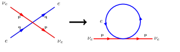
Figure 1: Forward scattering of neutrinos from the background particles involves no momentum exchange. These diagrams always add up coherently (i.e., at the amplitude level) and dominate over the other diagrams which add up incoherently (i.e., at the probability level). They manifest themselves as an effective mass which is well defined in the weak interaction basis.

In the free-streaming regime outside of the proto-neutron star the only important effect is scattering, which can significantly modify the flavor evolution of neutrinos. The scattering of neutrinos from each other and from other background particles should be discussed separately because in the former case identical particle effects play an important role. In a general astrophysical environment (as opposed to, say, a periodic crystal), scattering amplitudes from different background particles into a given direction generally add up incoherently, so their combined effect increases only linearly with the density of background particles. However, in the forward direction, scattering amplitudes from different background particles always add up coherently, in which case their combined effect increases quadratically with the background density. Therefore, in a dense environment, it is enough to work with an effective Hamiltonian which only includes the forward scattering terms in which there is no momentum transfer between neutrinos and the background particles Wolfenstein (1978); Barger et al. (1980) (also see Ref. Langacker et al. (1983)). When averaged over the background, such terms manifest themselves in the form of an effective mass (Fig. 1). The total mass includes both the effective mass which is diagonal in the weak interaction basis ($\nu_{e}$, $\nu_{x}$) and the ordinary neutrino mass which is diagonal in the mass basis ($\nu_{1}$, $\nu_{2}$), and it can be diagonalized in a new basis, which is called the matter basis ($\tilde{\nu}_{1}$, $\tilde{\nu}_{2}$). Therefore, the net effect of the background particles is to modify the mixing angle into a corresponding matter effective value. (For a review, see Ref. Kuo and Pantaleone (1989)). These effective mixing parameters depend on the background density and they vary as the neutrinos move from the inner dense regions of the supernova into to outer layers. However, if the density does not change significantly in the region of a few hundred kilometers outside of the proto-neutron star where the collective neutrino oscillations occur, one can assume that the effective mixing parameters are approximately constant. This would be a good approximation for the cooling period of the proto-neutron star since the shock wave is far away from its surface at those later times. (See Ref. Janka et al. (2007) for a review.) However, at earlier times, the changes in the density profile just outside of the proto-neutron star are more dramatic. In this paper, our methods and conclusions are independent of the actual values of the (effective) mixing parameters, as long as they can be considered constant. In particular, the Richardson-Gaudin diagonalization method depends on the constant density assumption in its present form. In what follows, our notation will refer to the vacuum values of the mixing parameters, but they can be easily exchanged with constant matter effective values.

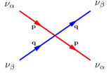
(a)            

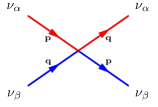
(b)            

Figure 2: Forward (a) and exchange (b) diagrams which add up coherently in $\nu\nu$ scattering.

When the scattering of neutrinos from each other is considered, in addition to those diagrams which involve no momentum transfer (forward scattering diagrams discussed above), those diagrams which involve a complete momentum exchange between neutrinos also add up coherently (Fig. 2) Pantaleone (1992a, b). This is due to the fact that, these diagrams can also be viewed as forward scattering diagrams in which neutrinos exchange their flavors. The effect of the exchange diagrams cannot be included in the form of effective mixing parameters as in the case of forward scattering. In fact, with the inclusion of the exchange diagrams, the problem turns into a many-body phenomenon because the flavor transformation of each neutrino is now affected by the flavor evolution of the entire neutrino ensemble.

The effective Hamiltonian which describes the forward scattering and exchange diagrams between neutrinos is given by Sawyer (2005); Pehlivan et al. (2011)

$$H_{\nu\nu} = \frac{G_{F}}{\sqrt{2}V}\sum_{\mathbf{p}}\sum_{\mathbf{q}}\left(1-\hat{\mathbf{p}}\cdot\hat{\mathbf{q}}\right)\left\{a^{\dagger}_{e}(\mathbf{p})a_{e}(\mathbf{p})a^{\dagger}_{e}(\mathbf{q})a_{e}(\mathbf{q})\right.$$ (24)

$$+a^{\dagger}_{x}(\mathbf{p})a_{x}(\mathbf{p})a^{\dagger}_{x}(\mathbf{q})a_{x}(\mathbf{q})+a^{\dagger}_{x}(\mathbf{p})a_{e}(\mathbf{p})a^{\dagger}_{e}(\mathbf{q})a_{x}(\mathbf{q})$$

$$\left.+a^{\dagger}_{e}(\mathbf{p})a_{x}(\mathbf{p})a^{\dagger}_{x}(\mathbf{q})a_{e}(\mathbf{q})\right\}$$

where the first two terms in the curly brackets correspond to the forward scattering diagrams shown in Fig. 2(a) whereas the last two terms represent the exchange diagrams shown in Fig. 2(b). In writing this Hamiltonian, the space coordinates are integrated out with the assumption of spacial uniformity, so one effectively works with neutrino plane waves. Neutral current interactions between neutrinos are treated with the Fermi 4-point interaction scheme and $G_{F}$ denotes the Fermi constant. This description is accurate for the MeV scale energies relevant for the supernova neutrinos. We assume that neutrinos are quantized in a box with volume $V$ so that the momentum $\mathbf{p}$ and its direction $\hat{\mathbf{p}}$ can take discrete values. As we follow the neutrinos in the comoving frame from the surface of the proto-neutron star to the point where neutrino self-interactions become negligible, this box expands corresponding to a decreasing neutrino density. But since we ignore neutrino creation in the free-streaming regime, new momentum modes do not appear.

The relativistic factor $1-\hat{\mathbf{p}}\cdot\hat{\mathbf{q}}$ in the Hamiltonian of Eq. (24) implies that relativistic neutrinos traveling along parallel paths cannot scatter off each other. This term turns the flavor evolution of a neutrino into a function of its direction of travel and significantly complicates the problem. Replacing this term with an average constant value results in the so called single angle approximation in which neutrinos are assumed to undergo identical flavor evolutions regardless of their direction. In this paper, we adopt the single angle approximation together with the neutrino bulb model Duan et al. (2006) which approximately accounts for the fact that the average value of the angle between the neutrinos, and hence the factor $1-\hat{\mathbf{p}}\cdot\hat{\mathbf{q}}$, decreases with the distance $r$ from the center of the supernova by replacing the latter with

$$1-\hat{\mathbf{p}}\cdot\hat{\mathbf{q}}\approx D(r)=\frac{1}{2}\left(1-\sqrt{1-\frac{r^{2}}{R_{\nu}^{2}}}\right)^{2}.$$ (25)

Here $R_{\nu}$ denotes the radius of the neutrino-sphere which is an imaginary sphere just inside the surface of the proto-neutron star from which neutrinos thermally decouple and start free streaming. In principle, $R_{\nu}$ is a function of time, and it decreases from almost $100$ km at the time of the bounce to about $10$ km at late times Roberts and Reddy (2016). However, the character of collective neutrino oscillations does not depend strongly on the value of $R_{\nu}$ Duan and Friedland (2011).

Using this approximation scheme, and the neutrino isospin operators given in Eq. (5) together with the adopted summation conventions, one can write the Hamiltonian in Eq. (24) as

$$H_{\nu\nu}=\mu(r)\vec{J}\cdot\vec{J}$$ (26)

where we discard some terms which are proportional to the total number of neutrinos in accordance with the discussion following Eq. (20). We also use the fact that scalar quantities have the same form in both mass and flavor bases, i.e., $\vec{J}\cdot\vec{J}=\vec{J}{\mbox{\tiny flavor}}\cdot\vec{J}{\mbox{\tiny flavor}}$. In Eq. (26),

$$\mu(r)=\frac{\sqrt{2}G_{F}}{V}D(r)$$ (27)

plays the role of an effective interaction constant. Since the normalization volume $V$ is inversely proportional to the neutrino density, it increases as $r^{2}$ with distance from the proto-neutron star. Together with the change of the average angle between the neutrinos in accordance with Eq. (25), $\mu(r)$ decreases roughly as ${1}/{r^{4}}$. The total Hamiltonian of an ensemble of neutrinos undergoing vacuum oscillations and self-interactions is found by adding Eqs. (21) and (26):

$$H=\sum_{\omega}\omega\hat{B}\cdot\vec{J}_{\omega}+\mu(r){\vec{J}}\cdot{\vec{J}}.$$ (28)

In the rest of this paper, we work with this Hamiltonian.

It was already pointed out by several authors that Eq. (28) is analogous to the Hamiltonian of a hypothetical one-dimensional spin system with long-range interactions in the presence of a position-dependent external magnetic field, given by

$$H_{\mbox{\tiny spin}}=\sum_{i}H_{i}\;\hat{B}\cdot\vec{S}_{i}+G(t){\vec{S}}\cdot{\vec{S}}.$$ (29)

Here, $i$ is a discrete position parameter in one dimension, and it is assumed that a (real) spin $\vec{S}_{i}$ is located at that point. The external magnetic field everywhere points in the direction of $\hat{B}$, while its magnitude $H_{i}$ at $i$ may be position dependent. In Eq. (29), $\vec{S}=\sum_{i}\vec{S_{i}}$ denotes the total spin of the system. It appears in the Hamiltonian because the range of the spin-spin interactions is assumed to be infinite, so every spin in the system interacts with every other one with the same strength. The analogy of this problem with the self-interacting neutrinos is clear once one identifies the spin-up ($|\uparrow\rangle$) and spin-down ($|\downarrow\rangle$) states of the former with the isospin states of the latter as

$$|\uparrow\rangle\leftrightarrow|\nu_{1}\rangle\qquad|\downarrow\rangle\leftrightarrow|\nu_{2}\rangle.$$ (30)

The interaction strength $G(t)$ in Eq. (29) may depend on time $t$. In particular, in the context of the analogy with self-interacting neutrinos $G(t)$ is assumed to decrease with time. In this case the spins are strongly correlated at the beginning when $G$ is large, but their dynamics are dominated by the external field at later times when $G$ is small. This analogy gives us a nice picture of spectral splits because, under the adiabatic evolution conditions, the spins eventually align or antialign themselves with the magnetic field as their mutual interactions slowly cease. Since $\hat{B}$ points in the direction of $J_{z}$ in the isospin space (see Eqs. (LABEL:eq:isospin_mass) and (22)), the neutrinos end up in one of the mass (or matter) eigenstates after the collective oscillations cease Raffelt and Smirnov (2007a).

Correlated spin systems like the one described in Eq. (29) is a popular subject in many-body physics because several problems with internal $su(2)$ symmetries can be described in analogy with them. Besides the self interacting neutrinos considered here, another example is a system of fermions with pairing interactions. While neutrino isospin plays the role of the spins in the former case, this role is played by the so-called pair quasispin in the latter. As a result, an analogy also exists between self-interacting neutrinos, and fermions with pairing interaction whereby the neutrino isospin and the pair quasispin are the analogous quantities. However, this analogy does not imply that supernova neutrinos form pairs. As is explained below, it is a more subtle analogy which should only be thought of as a mathematical similarity.

Pairing interaction appears in several fermionic many-body systems. It was originally suggested by Bardeen, Cooper, and Schrieffer (BCS) in connection with their theory of superconductivity Bardeen et al. (1957) as an effective interaction between electrons in the presence of a lattice. Soon it was realized that pairing also plays an important role in the nuclear shell model as the residual interaction between nucleons Mayer (1950a, b). In trapped ultracold atomic systems, a pairing interaction can be created between fermionic atoms Bloch et al. (2008); Giorgini et al. (2008); Randeria and Taylor (2014), and its strength can be controlled via Feshbach resonances by changing the applied magnetic field Inouye et al. (1998). This is particularly important as it allows direct experimental access to the behavior of the many-body system as the interaction constant changes with time.

The pairing model is described by the Hamiltonian

$$H_{\mbox{\tiny pair}}=\sum_{k}\sum_{i}\epsilon_{k}c^{\dagger}_{ki}c_{ki}^{\phantom{\dagger}}-g(t)\sum_{kk^{\prime}}\sum_{ii^{\prime}}c^{\dagger}_{ki}c^{\dagger}_{\bar{k}i}c_{\bar{k}^{\prime}i^{\prime}}^{\phantom{\dagger}}c_{k^{\prime}i^{\prime}}^{\phantom{\dagger}}\hskip 0.5pt.$$ (31)

where $\epsilon_{k}$ denotes a group of possibly degenerate energy levels, with the index $i$ running over such degeneracies. These levels can be either empty or occupied by a pair of spin-up and spin-down fermions, which are created by the operators $c^{\dagger}_{ki}$ and $c^{\dagger}_{\bar{k}i}$, respectively. The interaction strength $g(t)$ is a function of time in general. The pair quasispin operators mentioned above are defined by

$$\begin{split}&K^{+}_{ki}=c^{\dagger}_{ki}c^{\dagger}_{\bar{k}i}\quad K^{-}_{ki}=c_{\bar{k}i}^{\phantom{\dagger}}c_{ki}^{\phantom{\dagger}}\\ &K^{z}_{ki}=\frac{1}{2}\left(c^{\dagger}_{ki}c_{ki}^{\phantom{\dagger}}-c_{\bar{k}i}^{\phantom{\dagger}}c^{\dagger}_{\bar{k}i}\right)\hskip 0.5pt,\end{split}$$ (32)

and satisfy the $SU(2)$ commutation relations given in Eq. (6), with $\vec{J_{\mathbf{p}}}$ replaced with $\vec{K}_{ki}$. These definitions reflect the use of the quasispin doublet

$$\left(\begin{array}[]{c}\uparrow\downarrow\mkern-23.0mu\textrm{---}\\ \textrm{---}\end{array}\right)$$ (33)

in which an empty level $|\textrm{---}\rangle$ is defined to have quasispin down while an occupied level $|\uparrow\downarrow\mkern-23.0mu\textrm{---}\rangle$ is defined to have quasispin up. Defining a summation convention analogous to the ones introduced for neutrinos whereby $\vec{K}_{k}$ denotes the isospin operator which is summed over the degeneracy index $i$, and $\vec{K}$ denotes the total isospin operator summed over the index $k$, we can write the Hamiltonian in Eq. (31) as

$$H_{\mbox{\tiny pair}}=\sum_{k}2\epsilon_{k}K^{z}_{k}-g(t)\vec{K}\cdot\vec{K}\hskip 0.5pt.$$ (34)

In writing this Hamiltonian, we assume that the system contains a definite number of pairs, and discard a constant term related to this number. The similarity with the previous models becomes apparent with the identification

$$|\uparrow\downarrow\mkern-23.0mu\textrm{---}\rangle\leftrightarrow|\uparrow\rangle\leftrightarrow|\nu_{1}\rangle\qquad|\textrm{---}\rangle\leftrightarrow|\downarrow\rangle\leftrightarrow|\nu_{2}\rangle$$ (35)

The pairing problem was solved in the 1960s by Richardson Richardson (1963); Richardson and Sherman (1964); Richardson (1966) who was able to analytically write down the exact eigenstates and eigenvalues of the Hamiltonian given in Eq. (34). His solution was based on the Bethe ansatz technique Bethe (1931). In this method, one first forms a trial eigenstate depending on some unknown parameters and then tries to determine the values of these parameters by substituting the state into the eigenvalue-eigenstate equation. This process yields a coupled set of algebraic equations in the unknown parameters which are known as the Bethe ansatz equations. In 1976, also using the Bethe ansatz technique, Gaudin Gaudin (1976) solved a family of interacting spin model Hamiltonian’s which are today known as the (rational) Gaudin magnet Hamiltonians. These Hamiltonians were, at first glance, unrelated to the spin Hamiltonian given in Eq. (29), but Gaudin found the same Bethe ansatz equations as Richardson. In 1997, unaware of both Richardson’s and Gaudin’s work, Cambiaggio, Rivas, and Saraceno Cambiaggio et al. (1997) showed that the Gaudin magnet Hamiltonians are in fact constants of motion of the pairing Hamiltonian given in Eq. (31) corresponding to its dynamical symmetries. Today, we have a complete picture in which (a larger class of) Gaudin magnet Hamiltonians, and all models which are related or analogous to them, can be solved exactly by using the Bethe ansatz technique. For a review, see Ref. Dukelsky et al. (2004).

The analogy between self-interacting neutrinos, and the fermions with pairing interaction was first pointed out in Ref. Pehlivan et al. (2011), where the Richardson-Gaudin solution was used to obtain the exact many-body eigenstates and eigenvalues of the neutrino Hamiltonian given in Eq. (28). It was also pointed out that the Gaudin magnet Hamiltonians mentioned above form a set of invariants for the collective neutrino oscillations. (These invariants were also mentioned in Ref. Raffelt (2011) at the mean field level.) Reference Pehlivan et al. (2011) also showed that, at the mean field level, and for an initial box distribution of electron neutrinos, the formation of a spectral split can be viewed as the evolution of relevant fermionic degrees of freedom from quasiparticle to particle degrees of freedom in the pairing model. A more recent study Pehlivan et al. (2017) found that, again at the mean field level, but for a more generic initial energy distribution of electron neutrinos, formation of a spectral split is analogous to the BCS-Bose Einstein condensation (BEC) crossover which was experimentally observed in cold atom systems Zwierlein et al. (2004); Bloch et al. (2008); Giorgini et al. (2008); Randeria and Taylor (2014). Here we will further exploit the analogy between self interacting neutrinos and the fermions with pairing interaction to show, for the first time, the emergence of a spectral split in the exact many-body picture.

III Eigenstates in special cases

The Bethe ansatz method can be applied to the neutrino Hamiltonian for any value of the interaction constant $\mu$. However, in the limits of strongly and weakly interacting systems, one can find the eigenstates and eigenvalues by conventional methods as well. For the sake of an intuitive understanding, it is useful to study these limits first before we apply the Richardson-Gaudin diagonalization for the arbitrary values of the interaction constant.

III.1 Eigenstates at $\mu\to 0$ limit

When the neutrino density is very low, as would be the case when neutrinos are far from the center of the supernova, the self-interaction term of the Hamiltonian in Eq. (28) can be ignored. In this case, the Hamiltonian only consists of the vacuum oscillation terms:

$$\lim_{\mu\to 0}H=\sum_{\omega}\omega\hat{B}\cdot\vec{J}_{\omega}=-\sum_{\omega}\omega J_{\omega}^{z}.$$ (36)

Since there is no coupling between different oscillation modes in this limit, the eigenstates of the Hamiltonian are tensor products of the eigenstates of individual isospin components $J_{\omega}^{z}$. In other words, they can be written as

$$\prod_{\omega}|j_{\omega},m_{\omega}\rangle.$$ (37)

The eigenvalue corresponding to the state in Eq. (37) is given by

$$E=-\sum_{\omega}\omega m_{\omega}.$$ (38)

Note that since the total isospin quantum number $j_{\omega}$ can take several (degenerate) values ranging from $0$ or $1/2$ to $n_{\omega}/2$, the states $|j_{\omega},m_{\omega}\rangle$ form a reducible representation. However, in what follows, we will assume that $\vec{J}_{\omega}$ lives in the highest weight representation, i.e., $j_{\omega}=n_{\omega}/2$ for every $\omega$. This choice is dictated by the symmetries of our simplified model and the initial state. Our simplified Hamiltonian given in Eq. (28) does not include any dependence on the position, or propagation direction of the neutrinos. In fact, it remains unchanged if we exchange any two neutrinos with the same energy. Moreover, in this paper we restrict ourselves to the study of a neutrino ensemble which initially consists only of electron neutrinos; i.e., our initial state is completely symmetric under the exchange of any two neutrinos including those with different energies.Naturally the symmetry of the initial state between different energy modes will be broken by the vacuum oscillations once they start. But when the state evolves according to the Hamiltonian in Eq. (28), it will continue to be symmetric under the exchange of any two neutrinos with the same energy. Among the possible $|j_{\omega},m_{\omega}\rangle$ states, only those that live in the highest weight ($j_{\omega}=n_{\omega}/2$) representation satisfy this requirement. That is to say, only those states are invariant under the exchange of any two neutrinos with the same $\omega$. For this reason, although there are many more eigenstates of the Hamiltonian, the dynamics of our initial state is restricted to those which involve only the highest weight representation for each $\omega$.

Note that the total isospin quantum number $j$ of all neutrinos is not restricted by this symmetry. In accordance with Eq. (10), $j$ can take any value from $0$ up to $n/2$.

Instead of using the basis in which the isospins are summed for each $\omega$, one can also use the basis of individual neutrino isospins. Since the isospin being up or down corresponds to the neutrino being in the first or second mass eigenstate, respectively, the many-body eigenstates in Eq. (37) can also be written as

$$|\nu_{i_{1}},\nu_{i_{2}},\dotsc\nu_{i_{n}}\rangle$$ (39)

in the $\mu\to 0$ limit, where $i_{k}=1,2$. As per our discussion above, those neutrinos in the same oscillation modes should be symmetrized. The eigenstates in Eq. (39) are in a form that one would intuitively expect because neutrinos in mass eigenstates do not oscillate in vacuum and therefore form the stationary states of the Hamiltonian when there are no interactions. However, those eigenstates in Eq. (37) are more suitable for the Bethe ansatz scheme. These two sets of eigenstates are related by a set of complicated Clebsh-Gordon coefficients which will not be reproduced here.

III.2 Eigenstates at $\mu\to\infty$ limit

When neutrino density is sufficiently high so that $\mu$ is much larger than the relevant $\omega$ values in the system, one can ignore the vacuum oscillations in the Hamiltonian in Eq. (28):

$$\lim_{\mu\to\infty}H=\mu(r){\vec{J}}\cdot{\vec{J}}$$ (40)

This limit would be realized when the neutrinos are close to the proto-neutron star at the center. The eigenstates of the Hamiltonian in this limit are the $|j,m\rangle$ states of the total (mass) isospin with the eigenvalue $\mu j(j+1)$:

$$\lim_{\mu\to\infty}H|j,m\rangle=\mu j(j+1)|j,m\rangle$$ (41)

Here the total isospin quantum number $j$ can take any value from $0$ or $1/2$ to $n/2$. We emphasize once again that our assumption of highest weight representation applies only to the total isospin of individual oscillation modes $\vec{J}_{\omega}$, not to the total isospin $\vec{J}$.

The operator $U$ given in Eq. (12) converts the mass isospin states to flavor isospin states:

$$|j,m\rangle_{\mbox{\tiny flavor}}=U|j,m\rangle$$ (42)

This can be seen by summing Eq. (13) over all neutrinos, and using it on both sides of Eq. (42). The operator $U$ commutes with the Hamiltonian in Eq. (40), which tells us that the total flavor isospin states given in Eq. (42) are also eigenstates of the Hamiltonian with the same eigenvalue in the $\mu\to\infty$ limit. This can also be seen by noting that, when $U$ acts on $|j,m\rangle$, it cannot change the value of $j$. In other words, the right-hand side of Eq. (42) yields

$$|j,m\rangle_{\mbox{\tiny flavor}}=\sum_{m=-j}^{j}\alpha_{m}^{(j)}(z)|j,m\rangle$$ (43)

where $\alpha_{m}^{(j)}(z)$ are some coefficients that can be calculated from Eq. (12). Since all the states on the right-hand side of Eq. (43) are degenerate with energy $\mu j(j+1)$ in the $\mu\to\infty$ limit, the state on the left-hand side is also an eigenstate with the same energy in this limit.

IV Number Conservation and Classification of Eigenstates

Richardson-Gaudin diagonalization Richardson (1963); Richardson and Sherman (1964); Richardson (1966); Gaudin (1976) was applied to self-interacting neutrinos in Ref. Pehlivan et al. (2011), and the resulting eigenvalues were presented in their most generic form. In this section, we reproduce the relevant results of Ref. Pehlivan et al. (2011) both for the convenience of the reader and to set our notation. Here we restrict ourselves to only those eigenstates which meet our symmetry criteria, i.e., only those involving the highest weight representations $j_{\omega}=n_{\omega}/2$ for each $\omega$. (See the discussion following Eq. (38).)

The Hamiltonian in Eq. (28) commutes with the operator $\vec{B}\cdot\vec{J}=J^{z}$. In the interacting spin model analogy, this corresponds to the fact that the problem is unchanged if we rotate the spin system around the magnetic field. For neutrinos, it reflects the fact that we can multiply mass eigenstates with arbitrary phases without changing the Hamiltonian. Since $J_{z}$ commutes with the Hamiltonian, it can be diagonalized together with it; i.e., for an energy eigenket $|\psi_{E}\rangle$, we can always write

$$J_{z}|\psi_{E}\rangle=m|\psi_{E}\rangle.$$ (44)

In what follows we classify eigenstates of the Hamiltonian according to Eq. (44).

Using Eqs. (LABEL:eq:isospin_mass) and (17), together with the related summation conventions, we can write $J_{z}$ as

$$J^{z}=\frac{N^{(1)}-N^{(2)}}{2}.$$ (45)

Since we are in the free-streaming regime, the total number of neutrinos $N=N^{(1)}+N^{(2)}$ is also conserved. Together with Eq. (45), this tells us that $N^{(1)}$ and $N^{(2)}$ are separately conserved, and they can also be diagonalized together with the Hamiltonian. For the energy eigenket in Eq. (44) we can write

$$n^{(1)}=\frac{n}{2}+m\quad\mbox{and}\quad n^{(2)}=\frac{n}{2}-m.$$ (46)

For example, for those states with $(n^{(1)},n^{(2)})=(n,0)$ and $(n^{(1)},n^{(2)})=(0,n)$ the action of $J_{z}$ yields

$$m=\frac{n^{(1)}-n^{(2)}}{2}=\pm\frac{n}{2}$$ (47)

respectively. Therefore, these states can only belong to the $j=n/2$ representation. In fact, they are, respectively, the highest and lowest weight states of the total isospin given by

$$\begin{split}|n/2,+n/2\rangle&=\prod_{\omega}|\frac{n_{\omega}}{2},\;+\frac{n_{\omega}}{2}\rangle=|\nu_{1},\nu_{1},\dots,\nu_{1}\rangle\\ |n/2,-n/2\rangle&=\prod_{\omega}|\frac{n_{\omega}}{2},\;-\frac{n_{\omega}}{2}\rangle=|\nu_{2},\nu_{2},\dots,\nu_{2}\rangle.\end{split}$$ (48)

These are also the simultaneous eigenstates of ${\vec{J}}\cdot{\vec{J}}$ and $J^{z}_{\omega}$ with the respective eigenvalues $n/2(n/2+1)$ and $\pm\frac{n_{\omega}}{2}$. As a result, they are eigenstates of the total neutrino Hamiltonian for any value of $\mu$, i.e.,

$$H\;|n/2,\pm n/2\rangle=E_{\pm n/2}\;|n/2,\pm n/2\rangle$$ (49)

with

$$E_{\pm n/2}=\mp\sum_{\omega}\omega\frac{n_{\omega}}{2}+\mu\;\frac{n}{2}(\frac{n}{2}+1).$$ (50)

It is easy to understand intuitively why the two states in Eq. (48) are eigenstates of the Hamiltonian. A hypothetical ensemble of neutrinos which are all in mass eigenstates would not undergo vacuum oscillations. If, in addition, all of these neutrinos occupy the same mass eigenstate (i.e., all $\nu_{1}$ or all $\nu_{2}$), then the many-body state would also remain unchanged under the neutrino-neutrino interactions because both the forward and exchange diagrams would take the state onto itself.

V One Bethe ansatz variable

Other eigenstates of the Hamiltonian can be obtained with the Bethe ansatz technique. As mentioned earlier, this method is based on a trial state depending on some unknown parameters which are known as the Bethe ansatz variables. For our particular Hamiltonian, Bethe ansatz states are formed with the help of the so-called Gaudin algebra operators

$$\vec{Q}(\xi)=\sum_{\omega}\frac{\vec{J}_{\omega}}{\omega-\xi}.$$ (51)

Here $\xi$ is a generic complex number which will later turn into a Bethe ansatz variable and its value will be determined from the requirement that the trial state is an eigenstate.

Before we consider the most general case, it is instructive to study the simplest nontrivial application of the formalism in detail. For this purpose, we consider those eigenstates with $(n^{(1)},n^{(2)})=(1,n-1)$. These eigenstates yield

$$m=\frac{n^{(1)}-n^{(2)}}{2}=-\frac{n}{2}+1,$$ (52)

under the action of $J_{z}$. Therefore, they live in $j=n/2,n/2-1$ representations. In order to find their explicit form, one starts from the Bethe ansatz state

$$|\xi_{1}\rangle=Q^{+}(\xi_{1})|n/2,-n/2\rangle$$ (53)

where $Q^{+}(\xi_{1})$ is given by the + component of Eq. (51). Note that this state is not normalized, but the corresponding normalized state can be easily found as

$${|\xi_{1}\rangle}^{\prime}=\frac{1}{\sqrt{G}}Q^{+}(\xi_{1})|n/2,-n/2\rangle\hskip 0.5pt,$$ (54)

where

$$G=\sum_{\omega}\frac{1}{(\xi_{1}-\omega)^{2}}.$$ (55)

The non-normalized Bethe ansatz states in the form of Eq. (53) are usually more convenient to work with. In this paper, we mostly work with unnormalized eigenstates unless we specifically state otherwise. We denote the normalized eigenstates with a prime as in Eq. (54).

(a) Electrostatic analogy for the Bethe ansatz equation given in Eq. (58).

(b) Paths of two representative solutions of the Bethe ansatz equations as $\mu$ decreases from very large to very small values.

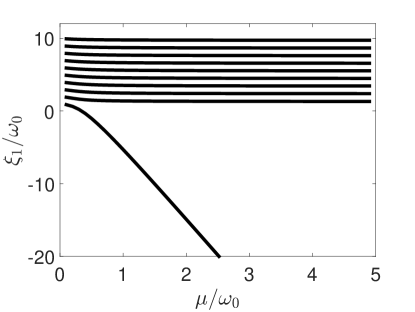
(c) Numerical solutions of the Bethe ansatz equation given in Eq. (58) for the toy model introduced in Eq. (74).

Figure 3: (a) The Bethe ansatz variable $\xi_{1}$ is interpreted as the position of a point particle with one unit of positive electric charge in the complex plane, while the neutrino oscillation frequencies $\{\omega_{1},\cdots,\omega_{n}\}$ are interpreted as the positions of fixed particles with negative charges $\{-j_{\omega_{1}},\cdots,-j_{\omega_{n}}\}$, respectively. The self-interaction constant $\mu$ enters the electrostatic picture as an external electric field. The equilibrium position of $\xi_{1}$ in this setup is the solution of Eq. (58). Although Bethe ansatz variables can be complex, in general, in the particular case of a single Bethe ansatz variable the solution is always real due to the symmetry of the problem around the $x$-axis. (b) If the equilibrium position of the free charge is at $-\infty$ in the $\mu\to\infty$ limit, then it approaches $\omega_{1}$ as $\mu\to 0$. If its equilibrium position is in between $\omega_{k}$ and $\omega_{k+1}$ for $k\geq 1$ in the $\mu\to\infty$ limit, then it approaches $\omega_{k+1}$ as $\mu\to 0$. We assume that $\omega_{1}<\omega_{2}<\dots<\omega_{\Omega}$. (c) Numerical solutions for the toy model introduced in Eq. (74) agree with these expectations. As $\mu$ decreases (from right to left in the figure), one of the solutions starts from $-\infty$ and approaches the lowest oscillation frequency, while the others start in between oscillation frequencies and approach the larger frequencies in their respective intervals.

In order to understand the trial state $|\xi_{1}\rangle$, first note that in $|n/2,-n/2\rangle$, all neutrinos are $\nu_{2}$. (See Eq. (48).) The operator $Q^{+}(\xi_{1})$ given in Eq. (54) turns one of these $\nu_{2}$ into a $\nu_{1}$ in such a way that the probability amplitude of finding this single $\nu_{1}$ in the oscillation mode $\omega$ is $1/(\sqrt{G}(\omega-\xi_{1}))$. We want to choose $\xi_{1}$ so that this state satisfies

$$H|\xi_{1}\rangle=E(\xi_{1})|\xi_{1}\rangle$$ (56)

for some energy $E(\xi_{1})$. A direct substitution of the state in Eq. (53) into the left-hand side of Eq. (56) yields

$$\begin{split}H|\xi_{1}\rangle\;=\;\;&(E_{-n/2}-\mu n-\xi_{1})|\xi_{1}\rangle\\ &\mkern-25.0mu-\left(1+2\mu\sum_{\omega}\frac{{-n_{\omega}}/2}{\omega-\xi_{1}}\right)J^{+}|n/2,-n/2\rangle\hskip 0.5pt.\end{split}$$ (57)

where $E_{-n/2}$ is the energy of the lowest weight state given in Eq. (50). A comparison between Eqs. (57) and (56) leads to the conclusion that $|\xi_{1}\rangle$ is an eigenstate of the Hamiltonian if one chooses $\xi_{1}$ so as to satisfy

$$-\frac{1}{2\mu}+\sum_{\omega}\frac{n_{\omega}/2}{\omega-\xi_{1}}=0.$$ (58)

Equation  (58) is a Bethe ansatz equation. Solving this equation for $\xi_{1}$ and substituting the solution retrospectively in Eq. (53) yields an exact eigenstate whose energy eigenvalue is given by

$$E(\xi_{1})=E_{-n/2}-\mu n-\xi_{1}\hskip 0.5pt.$$ (59)

In general, Bethe ansatz variables can take complex values. But in the particular case of a single Bethe ansatz variable, Eq. (58) admits only real solutions. Therefore, $\xi_{1}$ and the resulting energy given in Eq. (59) are always real.

In constructing the Bethe ansatz state given in Eq. (53), we started from the lowest weight (all $\nu_{2}$) state and converted one $\nu_{2}$ into a $\nu_{1}$. This is what we call a raising operator formulation. It is also possible to use the opposite lowering operator formalism by starting from the highest weight (all $\nu_{1}$) state and converting one $\nu_{1}$ into a $\nu_{2}$, i.e.,

$$|\zeta_{1}\rangle=Q^{-}(\zeta_{1})|n/2,n/2\rangle.$$ (60)

These eigenstates have $(n^{(1)},n^{(2)})=(n-1,1)$ and yield

$$m=\frac{n^{(1)}-n^{(2)}}{2}=\frac{n}{2}-1,$$ (61)

under the action of $J_{z}$. Therefore, they also live in $j=n/2,n/2-1$ representations of total isospin. Through direct substitution, one can show that the state in Eq. (60) is an eigenstate of the Hamiltonian with the energy

$$E(\zeta_{1})=E_{+n/2}-\mu n+\zeta_{1}\hskip 0.5pt,$$ (62)

if $\zeta_{1}$ obeys the Bethe ansatz equation

$$\frac{1}{2\mu}+\sum_{\omega}\frac{n_{\omega}/2}{\omega-\zeta_{1}}=0.$$ (63)

In Eq. (62), $E_{+n/2}$ denotes the energy of $|n/2,n/2\rangle$ and is given in Eq. (50).

Note that the Bethe ansatz equations for the raising and lowering formalisms (Eq. (58) and (63)) are the same except for the sign of the $1/2\mu$ term. In what follows, we discuss the solutions of the Bethe ansatz equations in the context of the raising operator formalism. Our conclusions also apply to the lowering operator formalism with appropriate sign changes.

In general, Bethe ansatz equations admit several solutions, each one yielding an eigenstate. In particular, for an $n$-particle system there should be $n$ linearly independent eigenstates with $(n^{(1)},n^{(2)})=(1,n-1)$. However, we restrict ourselves to those states which are completely symmetric under the exchange of any two neutrinos in the same oscillation mode. The number of such symmetric states with $(n^{(1)},n^{(2)})=(1,n-1)$ is equal to $\Omega$, i.e., the number of energy modes in the system. Therefore, we expect to find $\Omega$ eigenstates in the form of Eq. (53). Indeed it is easy to see that the number of solutions of Eq. (58) is $\Omega$. As discussed below, each one of these solutions yields a linearly independent eigenstate when substituted in Eq. (53). That these states satisfy the required symmetry condition is guaranteed by the fact that each $J_{\omega}^{+}$ in $Q^{+}(\xi_{1})$ lives in the highest weight representation $j_{\omega}=n_{\omega}/2$.

Although one can work out the solutions of the Bethe ansatz equations directly, it is often useful to refer to the so-called electrostatic analogy which was first suggested by Gaudin Gaudin (1968) and elaborated by Richardson Richardson (1977). This analogy is based on the observation that the Bethe ansatz equations can be interpreted as the stability conditions for an electrostatic system on a complex plane. Let us denote the real and imaginary axes of the complex plane by $x$ and $y$, respectively. In the electrostatic analogy, the Bethe ansatz variable $\xi_{1}=x_{1}+iy_{1}$ is interpreted as the position of a point particle which carries one unit of positive electric charge in the complex plane (see Fig 3(a)). The neutrino oscillation frequencies $\{\omega_{1},\cdots,\omega_{n}\}$ are interpreted as the positions of some fixed point electric charges with magnitudes $\{-j_{\omega_{1}},\cdots,-j_{\omega_{n}}\}$, respectively. Since the oscillation frequencies are real and positive in our case, the fixed charges are positioned along the positive $x$ axis. The whole system is placed in a uniform electric field in the $-x$ direction with a strength of $1/{2\mu}$. It can be shown that the electrostatic potential energy of such a configuration is proportional to

$$V \propto \frac{1}{2\mu}Re(\xi_{1})-\frac{1}{2\mu}\sum_{\omega}j_{\omega}\omega-\frac{1}{2}\sum_{\begin{subarray}{c}\omega,\omega^{\prime}\\ \omega\neq\omega^{\prime}\end{subarray}}j_{\omega}j_{\omega^{\prime}}\ln{|\omega-\omega^{\prime}|}$$ (64)

$$+ \sum_{\omega}j_{\omega}\ln{|\xi_{1}-\omega|}~{}.$$

The free charge comes to an equilibrium when the electrostatic potential energy reaches a local minimum, i.e., when $\partial V/\partial\xi_{1}=0$. It is easy to show that this equilibrium condition yields the Bethe ansatz equation given in Eq. (58). Note that the positions of the fixed charges and the external field are such that the total electric field in which the free charge moves is symmetric with respect to the $x$ axis. For this reason, the equilibrium position of the free charge lies on the $x$ axis for any value of $\mu$. This is another way of saying that the Bethe ansatz equations given in Eq. (58) can only have real solutions.

We find the electrostatic analogy particularly helpful in visualizing the transformation of eigenstates with changing $\mu$. In what follows, we first consider the solutions of the Bethe ansatz equations and the corresponding eigenstates in the $\mu\to\infty$ and $\mu\to 0$ limits, respectively. Our aim is to show that they indeed agree with those discussed in Sec. III. Then we discuss how these eigenstates transform into each other as $\mu$ changes between these two limits.

${\bm{\mu}\to\infty}$ limit: In the limit where $\mu$ is very large, the external electric field in the analogy becomes very weak. In this limit, the stable configurations of the free charge $\xi_{1}$ lie either at $-\infty$ or in between the fixed charges (Fig. 3(b)). Since there is always an electric field in the $-x$ direction, even if it is vanishingly small, we do not have a stable solution at $+\infty$. Considering that there are $\Omega-1$ intervals between fixed charges, the total number of solutions is $\Omega$, as was mentioned earlier.

In Sec. III.2 we mentioned that in the $\mu\to\infty$ limit the Hamiltonian is proportional to ${\vec{J}}\cdot{\vec{J}}$ so the eigenstates must approach $|j,m\rangle$. Can we tell which $|j,m\rangle$ states these $\Omega$ solutions correspond to? The hint lies in Eq. (52) which tells us that for the states with one Bethe ansatz variable, total isospin quantum number $j$ can take only two values: $j=n/2$ or $j=n/2-1$. Therefore, the states $|\xi_{1}\rangle$ can only be related to

$$\underbrace{|\frac{n}{2},\;-\frac{n}{2}+1\rangle}_{\mbox{\tiny unique}}\quad\mbox{and}\quad\underbrace{|\frac{n}{2}-1,\;-\frac{n}{2}+1\rangle}_{(\Omega-1)-\mbox{\tiny fold degenerate}}\quad$$ (65)

and will go to one of these states in the $\mu\to\infty$ limit. Since $j$ is found by adding the individual $j_{\omega}$’s of $\Omega$ different oscillation modes, $j=n/2-1$ is $(\Omega-1)$-fold degenerate while $j=n/2$ is unique. One naturally suspects that in the $\mu\to\infty$ limit, the unique $\xi_{1}\to-\infty$ solution yields the unique $|n/2,n/2-1\rangle$ state, while $\Omega-1$ finite solutions between fixed charges correspond to the $\Omega-1$ states in the form of $|n/2-1,n/2-1\rangle$. This is indeed the case as can be shown very easily. For the $\xi_{1}\to-\infty$ solution, we can ignore the finite $\omega$ values in Eq. (58). This tells us that $\xi_{1}$ approaches $-\infty$ as

$$\xi_{1}\to-2\mu\sum_{\omega}\frac{n_{\omega}}{2}=-\mu n.$$ (66)

Therefore, Eq. (59) gives the corresponding energy eigenvalue as

$$\lim_{\mu\to\infty}E(\xi_{1})=\mu\frac{n}{2}(\frac{n}{2}+1)$$ (67)

in agreement with our guess that $\xi_{1}\to-\infty$ solution yields the $|\frac{n}{2},\;-\frac{n}{2}+1\rangle$ state. For those solutions in which $\xi_{1}$ remains finite, one can compute the energy from Eq. (59) by ignoring $\xi_{1}$ and $\omega$ with respect to $\mu$. The result is

$$\lim_{\mu\to\infty}E(\xi_{1})=\mu(\frac{n}{2}-1)\frac{n}{2}$$ (68)

confirming our guess that these solutions yield the $|\frac{n}{2},\;-\frac{n}{2}+1\rangle$ states. Technically, this only proves that finite $\xi_{1}$ solutions yield linear combinations of $|\frac{n}{2},\;-\frac{n}{2}+1\rangle$ states since they all have the same energy in the $\mu\to\infty$ limit. However, any linear combination of $j=n/2-1$ representations is a $j=n/2-1$ representation itself, and we can always choose the appropriate combinations of these representations so that each finite $\xi_{1}$ solution yields a single $|\frac{n}{2},\;-\frac{n}{2}+1\rangle$ state. See the Appendix for a further discussion of this point.

${\bm{\mu}\to 0}$ limit: In the limit where $\mu$ approaches zero, the external electric field in the analogy becomes very large. In such a large external field, the free charge can find a stable configuration only when it is practically on top of one of the fixed charges. This can also be seen easily from Eq. (58): When $\mu\to 0$, the Bethe ansatz equation can only be satisfied if $\xi_{1}$ approaches one of the oscillation frequencies, say $\tilde{\omega}$. In this limit, the Gaudin operator given in Eq. (51) diverges. In particular, we can write

$$(\tilde{\omega}-\xi_{1})Q^{+}(\xi_{1})\underset{\xi_{1}\to\tilde{\omega}}{\longrightarrow}{J^{+}_{\tilde{\omega}}}$$ (69)

which tells us that

$$(\tilde{\omega}-\xi_{1})|\xi_{1}\rangle\underset{\xi_{1}\to\tilde{\omega}}{\longrightarrow}{J^{+}_{\tilde{\omega}}}\prod_{{\omega^{\prime}}}|\frac{n_{\omega^{\prime}}}{2},-\frac{n_{\omega^{\prime}}}{2}\rangle$$ (70)

where we used Eqs. (48) and (53). We can get rid of the coefficient on the left-hand side by normalizing both sides of Eq. (70), which yields

$$|\xi_{1}\rangle^{\prime}\underset{\mu\to 0}{\longrightarrow}|\frac{n_{\tilde{\omega}}}{2},-\frac{n_{\tilde{\omega}}}{2}+1\rangle\prod_{{\omega^{\prime}(\neq\tilde{\omega})}}|\frac{n_{\omega^{\prime}}}{2},-\frac{n_{\omega^{\prime}}}{2}\rangle$$ (71)

where the prime indicates the normalized state (see Eq. (54)). The resulting state in Eq. (71) is clearly in the form of Eq. (37). Note that Eq. (71) corresponds to a state in which all oscillation modes contain only $\nu_{2}$ neutrinos, except for the mode $\tilde{\omega}$, which contains a single neutrino in $\nu_{1}$ and $n_{\tilde{\omega}}-1$ neutrinos in $\nu_{2}$.

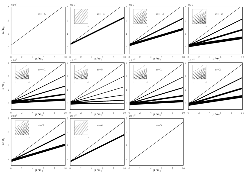
Figure 4: Energy eigenvalues of the Hamiltonian as a function of $\mu/\omega_{0}$. Vacuum frequencies are taken as $\omega_{i}=i\omega_{0}$. Each graph represents the states with different numbers of Bethe ansatz parameters, so each figure has a different eigenvalue of $J^{z}$ from $m=-5$ to $m=5$. At high densities, one can see that energy eigenvalues have a slope of $j(j+1)$ and are grouped by the length of total isospin as $j=5,4,3,2,1,0$. One important result from the figures is that level crossings appear between all states except the highest level state in the low density region.

Transformation of eigenstates: Which eigenstates in the $\mu\to\infty$ limit transform to which ones in the $\mu\to 0$ limit as $\mu$ decreases? It was already mentioned that the equilibrium position of the free charge has to be on the $x$ axis for all $\mu$ values. Suppose that the free charge is in equilibrium at $\xi_{1}\to-\infty$ in the $\mu\to\infty$ limit. As $\mu$ decreases and the electric field becomes stronger, this equilibrium position has to shift until it is on top of one of the free charges. However, since $\xi_{1}$ can never be imaginary, by shifting on the $x$ axis it can only end up on top of the lowest oscillation frequency $\omega_{1}$ in the $\mu\to 0$ limit. (See Fig. 3(b) and note that we take $\omega_{1}<\omega_{2}<\dots<\omega_{\Omega}$.) On the other hand, if $\xi_{1}$ is in equilibrium in between two fixed charges $\omega_{k}$ and $\omega_{k+1}$ for $k\geq 1$ in the $\mu\to\infty$ limit, then its equilibrium position shifts towards the larger oscillation frequency $\omega_{k+1}$ as $\mu$ decreases. In the $\mu\to 0$ limit, this equilibrium position will be on top of $\omega_{k+1}$.

These considerations tell us that the eigenstate $|n/2,\;n/2-1\rangle$ in the $\mu\to\infty$ limit transforms into the eigenstate given in Eq. (71) for $\tilde{\omega}=\omega_{1}$ as $\mu\to 0$. The corresponding eigenvalue transforms as

$$E(\xi_{1})=\begin{cases}\displaystyle{\mu\frac{n}{2}(\frac{n}{2}+1)},&\mbox{as }\mu\to\infty\\ &\\ \displaystyle{\omega_{1}(\frac{n_{\omega_{1}}}{2}-1)+\sum_{\omega(\neq\omega_{1})}\omega\frac{n_{\omega}}{2}},&\mbox{as }\mu\to 0.\end{cases}$$ (72)

On the other hand, the degenerate eigenstates $|n/2-1,\;n/2-1\rangle$ in the $\mu\to\infty$ limit turn into the eigenstates given in Eq. (71) for $\tilde{\omega}>\omega_{1}$ as $\mu\to 0$. The corresponding eigenvalues transform as

$$E(\xi_{1})=\begin{cases}\displaystyle{\mu(\frac{n}{2}-1)\frac{n}{2}},&\mbox{as }\mu\to\infty\\ &\\ \displaystyle{\tilde{\omega}(\frac{n_{\tilde{\omega}}}{2}-1)+\sum_{\omega(\neq\tilde{\omega})}\omega\frac{n_{\omega}}{2}},&\mbox{as }\mu\to 0\end{cases}$$ (73)

In order to illustrate these results, we consider a toy model with $10$ equally spaced and nondegenerate oscillation modes,

$$\omega_{i}=i\omega_{0}\qquad\mbox{for }i=1,2,\dots,10$$ (74)

where $\omega_{0}$ is an arbitrary oscillation frequency. The nondegeneracy assumption means that each mode contains only one neutrino so we have $n_{\omega_{i}}=1$ and $j_{\omega_{i}}=1/2$ for each $i$. The dimension of the corresponding Hilbert space is $2^{10}=1024$. In this particular example, we add $10$ isospin $1/2$’s, so the total isospin quantum number can take the values $j=5,4,3,2,1,0$ with the respective multiplicities of $1,9,35,75,90,42$. As per our classification scheme, we can discuss the eigenstates of the Hamiltonian by grouping them in terms of their eigenvalues under $J_{z}$, which can take the values $m=\pm 5,\pm 4,\pm 3,\pm 2,\pm 1,0$. Those states with $m=\pm 5$ are the trivial eigenstates discussed in Eq. (48). With one Bethe ansatz variable, we can obtain those eigenstates with $m=\pm 4$, depending on whether we use the raising or lowering formalism. Therefore, the only $j$ values which are relevant to us in this section are $j=5,4$. In this example, we only work with $m=-4$ states. Note that $m=+4$ states can be similarly studied with the lowering formalism.

Based on the above discussions we expect to find $10$ eigenstates with $m=-4$: One of these eigenstates should approach $|5,-4\rangle$ with its energy growing as $30\mu$ in the $\mu\to\infty$ limit. This state is expected to approach $|\nu_{1},\nu_{2},\nu_{2},\nu_{2},\nu_{2},\nu_{2},\nu_{2},\nu_{2},\nu_{2},\nu_{2}\rangle$ in the $\mu\to 0$ limit, while its energy approaches $53\omega_{0}/2$. The other nine eigenstates should approach $|4,-4\rangle$ in the $\mu\to\infty$ limit with their energies becoming degenerate and growing as $20\mu$. In the $\mu\to 0$ limit, we expect these states to be like the one given above, except that single $\nu_{1}$ will move to larger oscillation modes, i.e., $|\nu_{2},\nu_{1},\nu_{2},\nu_{2},\nu_{2},\nu_{2},\nu_{2},\nu_{2},\nu_{2},\nu_{2}\rangle$, $|\nu_{2},\nu_{2},\nu_{1},\nu_{2},\nu_{2},\nu_{2},\nu_{2},\nu_{2},\nu_{2},\nu_{2}\rangle$, $\dots$. The energies of these states will be $51\omega_{0}/2,49\omega_{0}/2,47\omega_{0}/2,\dots,35\omega_{0}/2$, respectively.

In Fig. 3(c) we show the numerical solutions of the Bethe ansatz equations given in Eq. (58). The behavior of the solution $\xi_{1}$ agrees with what we expect from the electrostatic analogy described above: One solution starts from $-\infty$ in the $\mu\to\infty$ limit and approaches the lowest oscillation frequency in the $\mu\to 0$ limit. The other solutions start in between the oscillation modes in the $\mu\to\infty$ limit and move towards the larger oscillation modes in their respective intervals. Corresponding energy eigenvalues calculated from Eq. (59) are shown in Fig. 4 on the panel marked with $m=-4$. The energy eigenvalue corresponding to the first solution mentioned above is the top line in this panel. As expected, it increases as $30\mu$ as $\mu\to\infty$, and becomes $53\omega_{0}/2$ as $\mu\to 0$. The energy eigenvalues corresponding to the other nine solutions increase as $20\mu$ as $\mu\to\infty$ and approach the values $51\omega_{0}/2,49\omega_{0}/2,47\omega_{0}/2,\dots,35\omega_{0}/2$ as $\mu\to 0$. The lowering formalism also yields $10$ solutions for $m=+4$ eigenstates. The energy eigenvalues corresponding to these solutions are shown in Fig. 4. Their behavior is qualitatively similar to (although not exactly the same as) the $m=-4$ case. The other panels of Fig. 4 show the energy eigenvalues of the states with other $m$ values which are discussed in the next section.

Note that our computation power in a standard desktop computer allows us to solve Bethe ansatz equations for up to $16$ neutrinos. However, since the resulting $2^{16}=65536$ eigenstates make our plots almost unreadable on paper, we choose to present a simpler example with $10$ neutrinos. Also, our choice of equally spaced and nondegenerate oscillation modes is due to its usefulness for a simple discussion. In our numerical simulations involving more than $10$ neutrinos occupying nonequally spaced modes, we do not see any behavior which is qualitatively different than this example.

VI More Bethe ansatz variables

The method outlined in the previous section can be generalized to obtain the eigenstates with generic occupation numbers. For example, let us consider those eigenstates with $(n^{(1)},n^{(2)})=(2,n-2)$. These eigenstates yield

$$m=\frac{n^{(1)}-n^{(2)}}{2}=-\frac{n}{2}+2,$$ (75)

under the action of $J_{z}$ which tells us that they live in $j=n/2,n/2-1,n/2-2$ representations of the total isospin. They can be computed by starting from a trial state with two Bethe ansatz parameters, i.e.,

$$|\xi_{1},\xi_{2}\rangle=Q^{+}(\xi_{1})Q^{+}(\xi_{2})|n/2,-n/2\rangle$$ (76)

The state $|n/2,-n/2\rangle$ has only $\nu_{2}$ neutrinos, but each one of the Gaudin operators turns one of them into a $\nu_{1}$. Note that $\xi_{1}$ which appears in this equation is not the same $\xi_{1}$ which appears in Eq. (53). Here, $\xi_{1}$ and $\xi_{2}$ are coupled with each other and satisfy a set of equations which is different from Eq. (58). This method of denoting the Bethe ansatz variables may be confusing at first. But since this is the standard notation in the literature, we adhere to it. Also note that the state in Eq. (76) is invariant under the exchange of the Bethe ansatz variables $\xi_{1}$ and $\xi_{2}$, i.e.,

$$|\xi_{1},\xi_{2}\rangle=|\xi_{2},\xi_{1}\rangle$$ (77)

because the operators $Q^{+}(\xi_{1})$ and $Q^{+}(\xi_{2})$ commute with one another.

As in the previous case, we derive the equations satisfied by $\xi_{1}$ and $\xi_{2}$ by requiring that $|\xi_{1},\xi_{2}\rangle$ is an eigenstate:

$$H|\xi_{1},\xi_{2}\rangle=E(\xi_{1},\xi_{2})|\xi_{1},\xi_{2}\rangle$$ (78)

Direct substitution of Eq. (76) into the left-hand side of Eq. (78) yields

$$\begin{split}&H|\xi_{1},\xi_{2}\rangle=-(\xi_{1}+\xi_{2}+2\mu n-2\mu+E_{-n/2})|\xi_{1},\xi_{2}\rangle\\ &\mkern-3.0mu-\mkern-3.0mu\left(1\mkern-5.0mu+\mkern-3.0mu2\mu\sum_{\omega}\frac{-n_{\omega}/2}{\omega-\xi_{2}}\mkern-3.0mu+\mkern-3.0mu\frac{2\mu}{\xi_{1}-\xi_{2}}\right)\mkern-3.0muQ^{+}(\xi_{1})J^{+}|n/2,-n/2\rangle\\ &\mkern-3.0mu-\mkern-3.0mu\left(1\mkern-3.0mu+\mkern-3.0mu2\mu\sum_{\omega}\frac{-n_{\omega}/2}{\omega-\xi_{1}}\mkern-3.0mu+\mkern-3.0mu\frac{2\mu}{\xi_{2}-\xi_{1}}\right)\mkern-3.0muQ^{+}(\xi_{2})J^{+}|n/2,-n/2\rangle\end{split}$$ (79)

For $|\xi_{1},\xi_{2}\rangle$ to be an eigenstate, we need to choose $\xi_{1}$ and $\xi_{2}$ in such a way that the last two terms on the right-hand side of Eq. (79) vanish. This yields a coupled set of two Bethe ansatz equations given by

$$\begin{split}&\sum_{\omega}\frac{-n_{\omega}/2}{\omega-\xi_{1}}=-\frac{1}{2\mu}+\frac{1}{\xi_{1}-\xi_{2}}\\ &\sum_{\omega}\frac{-n_{\omega}/2}{\omega-\xi_{2}}=-\frac{1}{2\mu}+\frac{1}{\xi_{2}-\xi_{1}}\end{split}$$ (80)

Solving these equations for $\xi_{1}$ and $\xi_{2}$, and substituting them retrospectively in Eq. (76) gives us an eigenstate with energy

$$E(\xi_{1},\xi_{2})=E_{-n/2}-\xi_{1}-\xi_{2}-2\mu(n-1)$$ (81)

In general the eigenstates with $(n^{(1)},n^{(2)})=(\kappa,n-\kappa)$ can be obtained by starting from a Bethe ansatz with $\kappa$ variables:

$$|\xi_{1},\xi_{2}\cdots,\xi_{\kappa}\rangle=Q^{+}(\xi_{1})\cdots Q^{+}(\xi_{\kappa})|n/2,-n/2\rangle$$ (82)

These states have

$$m=\frac{n^{(1)}-n^{(2)}}{2}=-\frac{n}{2}+\kappa,$$ (83)

telling us that they can live in $j=n/2,n/2-1,\dots,n/2-\kappa$ representations. It can be shown that the state in Eq. (82) is an eigenstate of the Hamiltonian with the energy

$$E(\xi_{1},\dotsc,\xi_{\kappa})=E_{-n/2}-\sum_{\alpha}^{\kappa}\xi_{\alpha}-\kappa\mu(n-\kappa+1)$$ (84)

if $\xi_{1}$,$\xi_{2}$,$\cdots$,$\xi_{\kappa}$ satisfy the following set of coupled Bethe ansatz equations:

$$\begin{split}&\sum_{\omega}\frac{-n_{\omega}/2}{\omega-\xi_{\alpha}}=-\frac{1}{2\mu}+\sum_{\beta\neq\alpha}^{\kappa}\frac{1}{\xi_{\alpha}-\xi_{\beta}}\\ &(\mbox{for every }\alpha=1,2,\dots,\kappa).\end{split}$$ (85)

When written out for every $\xi_{\alpha}$, Eq. (85) represents a set of $\kappa$ equations in $\kappa$ unknowns. As discussed below, these equations admit several solutions, each one yielding a linearly independent eigenstate when substituted in Eq. (82). Since the Bethe ansatz equations have real coefficients, each solution $(\xi_{1},\xi_{2},\dots,\xi_{\kappa})$ involves either real numbers, or complex conjugate pairs. As a result, the energy given in Eq. (84) is always real.

As we increase $\kappa$, (which increases $n^{(1)}$ and decreases $n^{(2)}$ such that $n=n^{(1)}+n^{(2)}$ remains constant) we need to solve a larger and larger system of coupled algebraic equations in order to find the relevant eigenstates. When we go from the states with $\kappa$ variables ($\xi_{1}$, $\xi_{2}$, $\dots$, $\xi_{\kappa}$) to the states with $\kappa+1$ variables ($\xi_{1}$, $\xi_{2}$, $\dots$, $\xi_{\kappa}$, $\xi_{\kappa+1}$), we need to solve the Bethe ansatz equations all over again because in the latter case the coupling to the variable $\xi_{\kappa+1}$ changes the values of the previous Bethe ansatz variables.

Bethe ansatz states presented above are not normalized. The norm of the general Bethe ansatz state given in Eq. (82) is equal to

$$\langle\xi_{1},\xi_{2}\cdots,\xi_{\kappa}|\xi_{1},\xi_{2}\cdots,\xi_{\kappa}\rangle=\det G(\xi_{1},\xi_{2}\cdots,\xi_{\kappa})$$ (86)

where $G(\xi_{1},\xi_{2}\cdots,\xi_{\kappa})$ is a $\kappa\times\kappa$ matrix whose elements are Zhou et al. (2002)

$$G_{\alpha\beta}=\left\{\begin{array}[]{l l}\sum_{\omega}\frac{1}{(\xi_{\alpha}-\omega)^{2}}-2\sum_{\alpha^{\prime}\neq\alpha}\frac{1}{(\xi_{\alpha}-\xi_{\alpha^{\prime}})^{2}}&\quad\text{if $\alpha=\beta$}\\ \frac{2}{(\xi_{\alpha}-\xi_{\beta})^{2}}&\quad\text{if $\alpha\neq\beta$}.\end{array}\right.$$ (87)

Therefore, corresponding normalized states can be written as

$${|\xi_{1},\cdots,\xi_{\kappa}\rangle}^{\prime}=\frac{1}{\sqrt{\det G}}Q^{+}(\xi_{1})\dotsc Q^{+}(\xi_{\kappa})|n/2,-n/2\rangle\hskip 0.5pt.$$ (88)

In order to find those eigenstates for which $n^{(1)}>n^{(2)}$, it is more economical to use the Bethe ansatz states constructed with lowering operators, i.e.,

$$|\zeta_{1},\zeta_{2}\cdots,\zeta_{\kappa}\rangle=Q^{-}(\zeta_{1})\cdots Q^{-}(\zeta_{\kappa})|n/2,n/2\rangle$$ (89)

which have

$$m=\frac{n^{(1)}-n^{(2)}}{2}=\frac{n}{2}-\kappa,$$ (90)

telling us that they also live in $j=n/2,n/2-1,\dots,n/2-\kappa$ representations. They can similarly be shown to be eigenstates of the Hamiltonian with the energy

$$E(\zeta_{1},\dotsc,\zeta_{\kappa})=E_{+n/2}-\sum_{\alpha}^{\kappa}\zeta_{\alpha}-\kappa\mu(n-\kappa+1)$$ (91)

if $\zeta_{1}$,$\zeta_{2}$,$\cdots$,$\zeta_{\kappa}$ satisfy

$$\begin{split}&\sum_{\omega}\frac{-n_{\omega}/2}{\omega-\zeta_{\alpha}}=\frac{1}{2\mu}+\sum_{\beta\neq\alpha}^{\kappa}\frac{1}{\zeta_{\alpha}-\zeta_{\beta}}\\ &(\mbox{for every }\alpha=1,2,\dots,\kappa).\end{split}$$ (92)

As for the case with one Bethe ansatz variable, the Bethe ansatz equations for the raising and lowering formalisms are identical except for a change in the sign of the $1/2\mu$ term. In what follows, we only discuss the solutions of the former, but our conclusions also apply to the latter with appropriate sign changes.

The electrostatic analogy introduced in Sec. IV can be generalized to any number of Bethe ansatz variables (See Fig. 5.) For $\kappa$ free particles carrying $+1$ unit of electric charge at positions $\xi_{\alpha}=x_{\alpha}+iy_{\alpha}$, the electrostatic potential energy is given by

$$V \propto \frac{1}{2\mu}\sum_{\alpha}Re(\xi_{\alpha})-\frac{1}{2\mu}\sum_{\omega}j_{\omega}\omega-\frac{1}{2}\sum_{\begin{subarray}{c}\alpha,\beta\\ (\alpha\neq\beta)\end{subarray}}\ln{|\xi_{\alpha}-\xi_{\beta}|}$$ (93)

$$- \frac{1}{2}\sum_{\begin{subarray}{c}\omega,\omega^{\prime}\\ \omega\neq\omega^{\prime}\end{subarray}}j_{\omega}j_{\omega^{\prime}}\ln{|\omega-\omega^{\prime}|}+\sum_{\alpha,\omega}j_{\omega}\ln{|\xi_{\alpha}-\omega|}~{}.$$

The free charges come to equilibrium when this electrostatic potential energy reaches a local minimum, i.e., when $\partial V/\partial\xi_{\alpha}=0$ is satisfied for every $\alpha$. It is easy to show that this equilibrium condition yields the Bethe ansatz equations given in Eq. (85). It was already mentioned above that the complex solutions of the Bethe ansatz equations always come as conjugate pairs. This is clearly visible in the electrostatic analogy: The positions of the fixed charges and the external electric field are such that the system can be in equilibrium only if the free charges distribute themselves symmetrically with respect to the $x$ axis.

Figure 5: Electrostatic analogy for the Bethe ansatz equations for more than one Bethe ansatz variables. Each Bethe ansatz variable $\xi_{\alpha}$ is interpreted as the position of a free point particle with one unit of positive electric charge. See the caption of Fig. 3

In what follows, we employ the electrostatic analogy to show that the Bethe ansatz states presented in this section agree with those presented in Secs III.1 and III.2 in the $\mu\to 0$ and $\mu\to\infty$ limits, respectively. After that we discuss how the eigenstates and eigenvalues transform into each other as $\mu$ decreases from very large to very small values.

${\bm{\mu}\to\infty}$ limit: The external electric field in the electrostatic analogy tends to zero in the $\mu\to\infty$ limit. Clearly there is a unique equilibrium solution in which all $\kappa$ free charges are in the $x\to-\infty$ region. There are also some equilibrium configurations in which $\kappa-1$ of the free charges are in the $x\to-\infty$ region while one free charge is located in between the fixed charges. Since interchanging Bethe ansatz variables does not change the corresponding Bethe ansatz state (see Eq. (77)), it does not matter which free charge is in the finite region. Therefore, the number of such configurations is $\Omega-1$ because there are $\Omega-1$ intervals in which the single free charge in the finite region can be located. We can continue in this manner to identify that equilibrium configurations with $\kappa-k$ free charges are at $x\to-\infty$, while $k$ free charges are located in the finite region near the free charges.

As mentioned in Sec III.2, the eigenstates of the Hamiltonian must approach $|j,m\rangle$ states of the total isospin in the $\mu\to\infty$ limit. From Eq. (83), we see that $j$ can only take the values $n/2\leq j\leq n/2-\kappa$. Therefore, the equilibrium configurations of the free charges mentioned above must yield the following states:

$$|\frac{n}{2},\;-\frac{n}{2}+\kappa\rangle\quad|\frac{n}{2}-1,\;-\frac{n}{2}+\kappa\rangle\quad\dots\quad|\frac{n}{2}-\kappa,\;-\frac{n}{2}+\kappa\rangle\quad$$ (94)

The corresponding energy eigenvalues should also approach $\mu j(j+1)$ at the same time. There is only one state with $j=n/2$ because the highest weight representation is unique. Inspired by our results in the previous section, we guess that this state is produced by the unique solution of the Bethe ansatz equations in which all $\kappa$ free charges are in the $x\to-\infty$ region. The number of states with $j=n/2-1$ is $\Omega-1$ which hints at the fact that these states are produced by the solutions in which $\kappa-1$ of the free charges are at $x\to-\infty$ while one of them is in between the fixed charges. In fact, it is very easy to analytically show that the following is true: the equilibrium configuration(s) in which $\kappa-k$ of the variables are located at the $x\to-\infty$ region while $k$ variables are located near the fixed charges in the $\mu\to\infty$ limit produce the states $|\frac{n}{2}-k,\;-\frac{n}{2}+\kappa\rangle$ for $k=0,1,\dots,\kappa$. This proof can be found in the Appendix.

${\bm{\mu}\to 0}$ limit: As $\mu$ becomes vanishingly small, the electric field in the electrostatic analogy becomes very strong. In that limit the free charges can find their equilibrium positions only on top of the fixed charges. Since free particles have $+1$ unit of electric charge while the fixed ones have $-n_{\omega}/2$ unit of charge, several free particles can end up on the same fixed particle. This can also be seen from the Bethe ansatz equations given in Eq. (85): As $\mu\to 0$, the divergence of the $1/2\mu$ term on the right-hand side can only be counteracted if $\xi_{\alpha}$ approaches one $\omega$, say $\tilde{\omega}^{(\alpha)}$. As a result, we can write

$$(\tilde{\omega}^{(\alpha)}-\xi_{\alpha})Q^{+}(\xi_{\alpha})\underset{\xi_{\alpha}\to\tilde{\omega}^{(\alpha)}}{\longrightarrow}{J^{+}_{\tilde{\omega}^{(\alpha)}}}$$ (95)

for the relevant Gaudin operator. Since Bethe ansatz equations in Eq. (85) have to be satisfied for every $\alpha=1,2,\dots,\kappa$, Eq. (95) is true for every $\xi_{\alpha}$. Therefore, we can write

$$\displaystyle{(\tilde{\omega}^{(1)}-\xi_{1})(\tilde{\omega}^{(2)}-\xi_{2})\dots(\tilde{\omega}^{(\kappa)}-\xi_{\kappa})|\xi_{1},\xi_{2},\dots,\xi_{\kappa}\rangle}$$

$$\displaystyle{\longrightarrow{J^{+}_{\tilde{\omega}^{(1)}}}{J^{+}_{\tilde{\omega}^{(2)}}}\dots J^{+}_{\tilde{\omega}^{(\kappa)}}\prod_{\omega}|\frac{n_{\omega^{\prime}}}{2},-\frac{n_{\omega^{\prime}}}{2}\rangle}$$ (96)

where we used Eqs. (48) and (82). The coefficients on the left-hand side drop when we normalize both sides of Eq. (VI). The result is

$$|\xi_{1},\xi_{2},\dots,\xi_{\kappa}\rangle^{\prime}\longrightarrow\prod_{\omega}|\frac{n_{\omega}}{2},m_{\omega}\rangle$$ (97)

where the values of $m_{\omega}$ depend on the particular equilibrium configuration reached, i.e., the values of $\tilde{\omega}^{(\alpha)}$. This state is in the form of Eq. (37), as expected.

Figure 6: (Color online) Real and imaginary parts of the solutions of Bethe ansatz equations for the simple example given in Eq. (74). These are the solutions which correspond to the highest energy eigenstates. All Bethe ansatz variables approach infinity as $\mu\to\infty$. At the $\mu\to 0$ limit they settle onto the vacuum oscillation frequencies beginning from the lowest one. This configuration yields the highest energy eigenstate at the $\mu\to 0$ limit. [See Eq. (98.)]. Note that for low values of $\mu$, complex conjugate Bethe ansatz variables approach each other and collide on the real axis, forming two distinct real solutions.

Transformation of Eigenstates: Now we are faced with the question of which eigenstate in the $\mu\to\infty$ limit transforms to which eigenstate in the $\mu\to 0$ limit as we change $\mu$. In general, this question is not as easy to answer for several Bethe ansatz variables as it is for a single variable. However, one key observation from our analysis of a single Bethe ansatz variable survives when we increase the number of Bethe ansatz variables: The highest energy eigenvalue of the Hamiltonian never becomes degenerate as we change $\mu$ from very large to very small values.

Let us first demonstrate this in the toy model with $10$ equally spaced oscillation modes considered in Sec V (See Eq. (74)) before giving a more general discussion about it. Out of the expected total of $1024$ eigenstates of this toy model, $1002$ have $m=\pm 3,\pm 2,\pm 1,0$ values which can be obtained with two, three, four, and five Bethe ansatz variables, respectively. We found all of the $1002$ solutions associated with these $m$ values by numerically solving the corresponding Bethe ansatz equations given in Eqs. (85) and (92). Our numerical solution utilizes the method introduced in Ref. Faribault et al. (2011). Since each solution involves several complex variables, it is impractical to present all of them here. In Fig. 4 we present the energy eigenvalues that we calculate by substituting these solutions in Eqs. (84) and (91). This figure also includes the eigenvalues of $m=\pm 4,\pm 5$ eigenstates for completeness. Note that $m=\pm 4$ eigenvalues were already discussed in the previous section and $m=\pm 5$ eigenvalues are taken from Eq. (48). Notice that for each $m$, the highest energy eigenvalue grows as $30\mu$ as expected from the fact that these states become $|5\;m\rangle$ in the $\mu\to 0$ limit.

In general, it is difficult to identify which eigenstate in the $\mu\to\infty$ limit is connected to which eigenstate in the $\mu\to 0$ limit from Fig. 4. As can be seen in the insets, the eigenvalues cross each other at several points in the low $\mu$ region. The only exceptions are the highest energy eigenvalues. For each $m$, the highest energy eigenvalue is distinctly nondegenerate for any value of $\mu$. Using this observation, it is possible to identify which state in the $\mu\to 0$ limit is connected to the state $|5,\;m\rangle$ in the $\mu\to\infty$ limit. All one needs to do is to identify the highest energy eigenstate at $\mu=0$ for a given value of $m$. As per Eq. (46) such a state should include $n^{(1)}=5+m$ neutrinos in the $\nu_{1}$ state and $n^{(2)}=5-m$ neutrinos in the $\nu_{2}$ state. Since having isospin-up (down) neutrinos at lower (higher) oscillation modes increases the energy, the highest energy state is found by placing all available $\nu_{1}$’s ($\nu_{2}$’s) in the lowest (highest) oscillation modes. This way one concludes that the states

$$|5,\;m\rangle\longleftrightarrow|\underbrace{\nu_{1},\dots,\nu_{1}}_{5+m},\underbrace{\nu_{2},\dots,\nu_{2}}_{5-m}\rangle$$ (98)

are analytically connected to each other through the running of $\mu$.

This can also be understood by examining the behavior of Bethe ansatz variables corresponding to the highest energy eigenvalues. In Fig. 6, we show the solutions in Eq. (85) with two, three, four, and five Bethe ansatz variables corresponding to the highest energy eigenstates with $m=-3,-2,-1,0$, respectively. (The solution with a single Bethe ansatz variable corresponding to the highest energy eigenvalue with $m=-4$ is already shown in the lowest line of Fig. 3(c).) As expected from the discussion above, these solutions are such that all variables start from the $x\to-\infty$ region when $\mu\to\infty$, yielding the maximum energy at this limit according to Eq. (84). As $\mu$ decreases, the Bethe ansatz variables approach the finite region and settle on top of the lowest possible vacuum oscillation frequencies. This configuration yields the maximum energy in the $\mu\to 0$ limit. According to Eqs. (VI) and (97), those neutrinos in the lowest oscillation modes are then converted to $\nu_{1}$, while those occupying the high oscillation modes remain $\nu_{2}$. This behavior is explicitly shown in Fig. 7 for five Bethe ansatz variables corresponding to the $m=0$ case. As can be seen in this figure, the free charges form an arc in the complex plane which closes in on the fixed changes as $\mu$ decreases.

Although we obtained Eq. (98) in the context of our simple example, the rest of this paper is based on the assumption that it is always true; i.e., the highest energy eigenvalues of the Hamiltonian for any value of $m$ never become degenerate so the states

$$|\frac{n}{2},\;m\rangle\longleftrightarrow|\underbrace{\nu_{1},\dots,\nu_{1}}_{\frac{n}{2}+m},\underbrace{\nu_{2},\dots,\nu_{2}}_{\frac{n}{2}-m}\rangle.$$ (99)

are analytically connected to each other by running $\mu$. We assume that this is true even when we allow more than one neutrino in the same oscillation mode. Whether or not the latter is allowed, the meaning of the right-hand side of Eq. (99) is clear: $\nu_{1}$’s fill up all available states starting from the lowest possible oscillation modes, and $\nu_{2}$’s fill up the rest. One oscillation mode in the middle can possibly contain both $\nu_{1}$ and $\nu_{2}$. In that case, they should be symmetrized as per our discussion below Eq. (38).

As mentioned in Sect. II, the neutrino Hamiltonian given in Eq. (28) and the pairing Hamiltonian given in Eq. (31) differ by an overall minus sign such that the highest energy eigenstates of the former (for different values of $m$) correspond to the ground states of the latter (for different numbers of pairs). The nondegeneracy of these states is a well-known phenomenon which is observed in numerical solutions of the Bethe ansatz equations under a variety of conditions. Although these solutions are studied in the context of fermion pairing in the literature, in what follows we discuss them using the language of self-interacting neutrinos. No general proof of Eq. (99) exists in the literature. However, a proof for large values of $n$ and $m$ is originally given by Gaudin Gaudin (1968), and later elaborated by Richardson Richardson (1977). This proof is based on the observation that as the number of Bethe ansatz variables ($\kappa$) increases, the solutions of the Bethe ansatz equations organize themselves into (piecewise) continuous arcs which are symmetric with respect to the $x$ axis in the electrostatic analogy. In particular, those solutions corresponding to the highest energy states on the left-hand side of Eq. (99) form a single continuous arc. As the interaction constant decreases and the external electrostatic field becomes stronger, this arc of free charges closes itself onto the line of fixed charges on the $x$ axis in order to find a stable configuration. During the transition the arc stays a single continuous structure. As a result, when it closes in on the line of fixed charges, the Bethe ansatz variables approach the lowest oscillation frequencies, converting the $\nu_{2}$’s in these modes into $\nu_{1}$’s. The resulting state is the rigth-hand side of Eq. (99). The analytical proofs of Gaudin and Richardson have been shown to agree with the numerical results for up to $n=1600$ and $\kappa=800$ in Ref. Roman et al. (2002) for the case of equally spaced oscillation modes similar to the one introduced in Eq. (74).

One can also discuss Eq. (99) from the point of view of experiments involving cold atomic systems. In such experiments where one can control the strength of the pairing interaction, the system is observed to move from very weak (BCS) to very strong (BEC) interaction regimes smoothly. This so-called crossover behavior indicates that the ground state of the system never undergoes a level crossing with one of the excited levels as it moves between these two limits. A level crossing would show itself as abrupt changes in the measurable quantities, which is not observed experimentally. This is true for any number of particle pairs which correspond to different $m$ values in the neutrino case, whether or not these pairs occupy degenerate energy levels. For a review, see Refs. Bloch et al. (2008); Giorgini et al. (2008); Randeria and Taylor (2014).

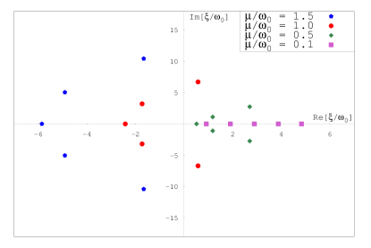
Figure 7: (Color online) The behavior of the five Bethe ansatz variables corresponding to the $m=0$ case as $\mu$ decreases. The free charges organize themselves into an arc in the complex plane which is symmetric with respect to the $x$ axis. As $\mu$ decreases, which increases the external electrostatic field, the arc of free charges closes in on the fixed charges. As $\mu\to 0$, the Bethe ansatz variables settle on the lowest oscillation modes.

VII Spectral Splits in Exact Many-Body Systems

In this section, we show that, under the assumption of perfect adiabaticity, the nondegeneracy of the highest energy eigenstates of the neutrino Hamiltonian for different $m$ values [cf. Eq. (99)] leads to a spectral split in the energy spectrum of a neutrino ensemble which initially consists of electron neutrinos only.

According to the adiabatic theorem, in a scenario in which $\mu$ changes sufficiently slowly with time, the time evolution of the highest energy eigenstates for each $m$ will be such that they will continue to occupy the same instantaneous eigenstates. In particular, apart from a phase, the state on the left-hand side of Eq. (99) will evolve into the state on the right-hand side as $\mu$ slowly decreases from very large to very small values under the adiabatic evolution conditions. Here we do not specify how slow is sufficiently slow. But the conditions for perfect adiabaticity are typically satisfied in a core collapse supernova Raffelt and Smirnov (2007a).

In the experimental setups involving cold atom systems, one can control how slowly the interaction constant changes with time, and ensure that the system stays in its ground state instead of being excited to the next energy level. In the case of neutrinos, one may intuitively think that, even if the perfectly adiabatic conditions are satisfied, the system would not stay on the highest energy eigenstate but would make a transition to a lower energy state. However, one should keep in mind that the neutrino system that we consider in Eq. (28) is dissipationless; i.e., the energy of the system is conserved.

Since $J_{z}$ is a conserved quantity of the problem, the adiabatic theorem can be applied to any combination of highest energy eigenstates for different $m$ values. In other words, based on Eq. (99), if the initial state at $\mu\to\infty$ is in the form

$$|\psi\rangle_{\mbox{\tiny initial}}=\sum_{m=-n/2}^{n/2}c_{m}|\frac{n}{2},m\rangle,$$ (100)

then, it will evolve into

$$|\psi\rangle_{\mbox{\tiny final}} =\mathcal{U}|\psi\rangle_{\mbox{\tiny initial}}$$ (101)

$$=\sum_{m=-n/2}^{n/2}c_{m}\phi_{m}|\underbrace{\nu_{1},\dots,\nu_{1}}_{\frac{n}{2}+m},\underbrace{\nu_{2},\dots,\nu_{2}}_{\frac{n}{2}-m}\rangle$$

in the $\mu\to 0$ limit. Here $\mathcal{U}$ denotes the evolution operator from the $\mu\to\infty$ limit to the $\mu\to 0$ limit under the adiabatic approximation, and $\phi_{m}$ are some phases which contain both dynamical and geometrical components associated with the adiabatic evolution. Their actual values are irrelevant for our purposes because they do not affect the final energy distributions.

Equations (100) and (101) are particularly useful when we consider an initial neutrino ensemble which consists entirely of electron neutrinos. Regardless of how many neutrinos each oscillation mode contains, such a state is the highest weight state in the flavor basis because all flavor isospins are up:

$$|\psi\rangle_{\mbox{\tiny initial}}=|\nu_{e},\nu_{e},\dotsc,\nu_{e}\rangle=|n/2,n/2\rangle_{\mbox{\tiny flavor}}$$ (102)

Using Eqs. (11) and (12), this state can be written as

$$|\psi\rangle_{\mbox{\tiny initial}}=U^{\dagger}|\nu_{1},\nu_{1},\dotsc,\nu_{1}\rangle$$ (103)

$$=\sum_{m=-n/2}^{n/2}(\cos\theta)^{(\frac{n}{2}+m)}(\sin\theta)^{(\frac{n}{2}-m)}\sqrt{n\choose{\frac{n}{2}+m}}|n/2,m\rangle.$$

Assuming that this state evolves adiabatically as described above, Eq. (101) tells us that it will turn into

$$|\psi\rangle_{\mbox{\tiny final}}= \sum_{m=-n/2}^{n/2}(\cos\theta)^{(\frac{n}{2}+m)}(\sin\theta)^{(\frac{n}{2}-m)}$$

$$\times\sqrt{n\choose{\frac{n}{2}+m}}\phi_{m}|\underbrace{\nu_{1},\dots,\nu_{1}}_{\frac{n}{2}+m},\underbrace{\nu_{2},\dots,\nu_{2}}_{\frac{n}{2}-m}\rangle$$ (104)

as $\mu\to 0$.

(a) Initial distribution

(b) Final distributions

Figure 8: (Color online) Adiabatic evolution of initial box distribution of electron neutrinos. This is the extension of the toy model that we introduced in Eq. (74). This time we consider $\Omega=10^{7}$ equally spaced oscillation modes each containing a single neutrino. We take $\omega_{0}=5\times 10^{-7}$ km^-1 and adopt the normal mass hierarchy with solar mixing parameters.

This final state is a superposition of $2n+1$ orthogonal components, each one with a split structure, i.e., filled by $\nu_{1}^{\prime}s$ up to a certain point and by $\nu_{2}$’s after that. In fact, for each one of these components, we can write

$$|\underbrace{\nu_{1},\dots,\nu_{1}}_{\frac{n}{2}+m},\underbrace{\nu_{2},\dots,\nu_{2}}_{\frac{n}{2}-m}\rangle=$$ (105)

$$(\prod^{s-1}_{k=1}|\frac{n_{\omega_{k}}}{2},\frac{n_{\omega_{k}}}{2}\rangle)(|\frac{n_{\omega_{s}}}{2},m_{\omega_{s}}\rangle)(\prod^{\Omega}_{k={s+1}}|\frac{n_{\omega_{k}}}{2},-\frac{n_{\omega_{k}}}{2}\rangle).$$

This equation is very simple to understand. It tells us that lower oscillation modes containing only $\nu_{1}$’s live in the highest weight states, while the higher oscillation modes containing only $\nu_{2}$’s live in the lowest weight states. A single oscillation mode labeled by $s$ may contain both types of neutrinos in a completely symmetrized way [see the discussion following Eq. (99)] and has $m_{\omega_{s}}=(n^{(1)}_{\omega_{s}}-n^{(2)}_{\omega_{s}})/2$. This particular mode can be found from the condition that

$$\sum_{k=1}^{s-1}n_{\omega_{k}}\leq\frac{n}{2}+m\leq\sum_{k=1}^{s}n_{\omega_{k}}$$ (106)

which simply tells us that the number of $\nu_{1}$’s on the left-hand side of Eq. (105) is more than enough to fill the first $s-1$ oscillation modes, but not enough to fill the $s{\mbox{th}}$ oscillation mode. We call $s$ the split index, and the corresponding frequency $\omega_{s}$ the split frequency. Clearly they both depend on the value of $m$. For this reason, in what follows we change the notation as

$$s\longrightarrow s(m)\quad\mbox{and}\quad\omega_{s}\longrightarrow\omega_{s(m)}$$ (107)

In fact, since the final state in Eq. (VII) contains components with all possible $m$ values, every allowed oscillation mode is a split frequency for one or more of these components. However, what we are interested in, is the normalized energy distributions given by

$$\Phi^{(\alpha)}(\omega)=\frac{1}{n}\;\langle N^{(\alpha)}(\omega)\rangle.$$ (108)

Here $\alpha$ can take values in $e,x,1,2$. The initial neutrino energy distributions can be easily written down in flavor basis as

$$\Phi^{(e)}_{\mbox{\tiny initial}}(\omega)=\frac{n_{\omega}}{n}\qquad\Phi^{(x)}_{\mbox{\tiny initial}}(\omega)=0.$$ (109)

This follows from the facts that the number of neutrinos in the oscillation mode $\omega$ is $n_{\omega}$, and the initial state in Eq. (103) contains nothing but electron neutrinos.

Final neutrino energy distributions are easiest to calculate in the mass basis. It is helpful to first note that Eq. (LABEL:eq:isospin_mass) leads to

$$N^{(a)}_{\omega}=\frac{n_{\omega}}{2}\pm J^{z}_{\omega}$$ (110)

where $a=1,2$. Here, and in what follows, we use the upper sign for $a=1$ and lower sign for $a=2$. Substituting Eq. (105) into Eq. (VII) and calculating the expectation value of $N^{(a)}_{\omega}$ using Eq. (110) leads to

$$\Phi^{(a)}(\omega_{k})=\frac{n_{\omega_{k}}}{2n}\pm\frac{1}{n}\sum_{m=-n/2}^{n/2} (\cos\theta)^{(n+2m)}(\sin\theta)^{(n-2m)}$$

$$\times{n\choose{\frac{n}{2}+m}}m_{\omega_{k}}$$ (111)

where

$$m_{\omega_{k}}=\begin{cases}\displaystyle{n_{\omega_{k}}/2},&\mbox{for }k<s(m)\\ \displaystyle{\frac{n^{(1)}_{\omega_{s(m)}}-n^{(2)}_{\omega_{s(m)}}}{2}},&\mbox{for }k=s(m)\\ \displaystyle{-n_{\omega_{k}}/2},&\mbox{for }k>s(m)\\ \end{cases}$$ (112)

in accordance with Eq. (105).

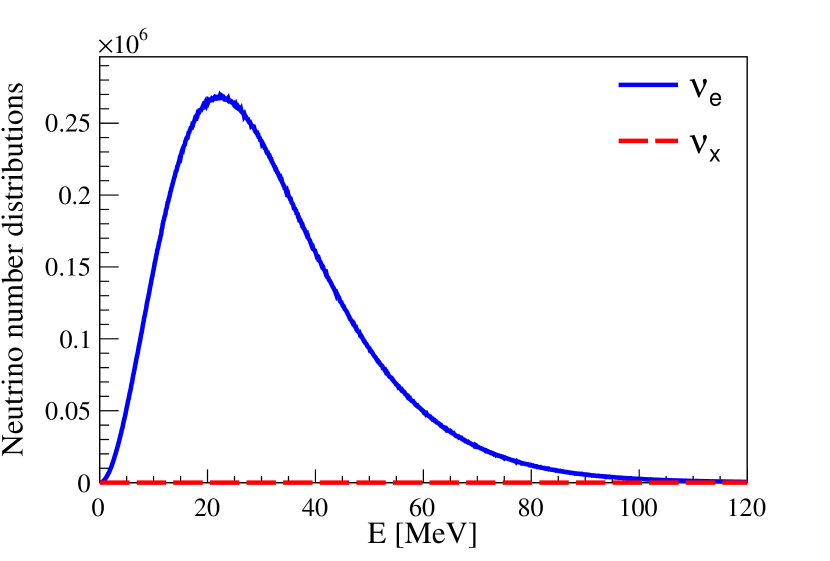
(a) Initial Fermi-Dirac distribution of electron neutrinos.

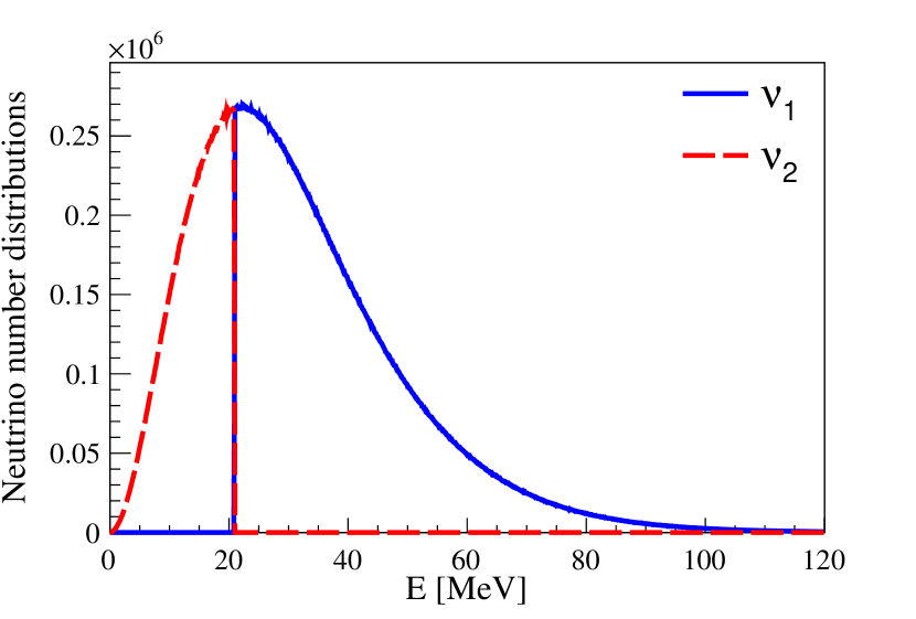
(b) Final distributions in mass basis.

Figure 9: (Color online) Adiabatic evolution of an initial thermal distribution of electron neutrinos. We take $n=10^{8}$ neutrinos distributed over $\Omega=1200$ oscillation modes which are equally spaced in energy [cf. Eq. (117)]. We take the temperature as $kT=10$ MeV, and adopt the normal mass hierarchy with solar mixing parameters. Note that, we use a pseudo-random number generator in order to distribute $n$ neutrinos into $\Omega$ energy bins according to Fermi-Dirac probability distribution. This guarantees that each energy bin has an integer number of neutrinos and a corresponding well-defined isospin quantum number. The use of the pseudo-random number generator causes the wiggles seen in the original distribution.

The calculation of the final energy distribution of neutrinos involves the numerical computation of Eqs. (VII) and (112). However, for the typical number of neutrinos that we work with, which extends up to $n=10^{8}$, it becomes impractical to directly calculate the factorials involved in the ${n\choose{\frac{n}{2}+m}}$ term. For this reason, we use the fact that

$$(\cos\theta)^{(n+2m)} (\sin\theta)^{(n-2m)}{n\choose{\frac{n}{2}+m}}$$

$$\approx\frac{1}{\sqrt{2\sigma^{2}\pi}}\exp\left({-\frac{\left(m-\bar{m}\right)^{2}}{2\sigma^{2}}}\right)$$ (113)

where

$$\bar{m}=n(\cos^{2}\theta-\frac{1}{2})\qquad\sigma=\sqrt{n}\cos\theta\sin\theta$$ (114)

The left-hand side of Eq. (VII) is nothing more than the binomial distribution, while the right-hand side is the Gaussian distribution with mean value $\bar{m}$ and standard deviation $\sigma$. These two distributions approximate very well to each other at the large $n$ values that we work with. Substituting Eq. (VII) into Eq. (VII) leads to the formula for the final neutrino energy distributions that we use in our numerical computations:

$$\Phi^{(a)}(\omega_{k})=$$ (115)

$$\frac{n_{\omega_{k}}}{2n}\pm\frac{1}{n}\sum_{m=-n/2}^{n/2}\frac{1}{\sqrt{2\sigma^{2}\pi}}\exp\left({-\frac{\left(m-\bar{m}\right)^{2}}{2\sigma^{2}}}\right)m_{\omega_{k}}$$

One can now calculate the final energy distribution by numerically computing $m_{\omega_{k}}$ from Eqs. (106) and (112) for a given initial distribution and by substituting them in Eq. (115).

The simplest case that one can consider is an extension of the toy model that we introduced in Eq. (74). This time we divide the interval into $\Omega=10^{7}$ equally spaced oscillation modes and allow each mode to contain only a single neutrino (i.e., $n_{\omega_{k}}=1$) so that the total number of neutrinos is $n=10^{7}$. This brings us to the continuum limit of this example. [See Fig. 8(a).] In this particular case, Eq. (112) is simply reduced to

$$m_{\omega_{k}}=\left\{\begin{array}[]{l l}-1/2&\quad\text{if $k>\frac{n}{2}+m$}\\ +1/2&\quad\text{otherwise}\end{array}\right.$$ (116)

whose substitution in Eq. (115) yields the final energy distribution shown in Fig. 8(b). In this example we take $\omega_{0}=5\times 10^{-7}$ km^-1. We adopt solar mixing parameters for demonstration purposes because a smaller mixing angle brings the split point in Fig. 9(b) too close to the edge of the distribution.

Next, we consider another example in which the electron neutrinos are initially in a thermal energy distribution, i.e., the fraction of neutrinos in the $(\omega,\omega+d\omega)$ interval is given by

$$\Phi^{(e)}_{\mbox{\tiny initial}}(\omega)d\omega=\frac{1}{(kT)^{3}\Gamma(3)F_{2}(0)}\frac{E^{2}dE}{e^{E/kT}+1}$$ (117)

Here $k$, $\Gamma$, and $F_{2}$ denote the Boltzmann constant, the Gamma function and the complete Fermi-Dirac integral of rank 2, respectively. The variables $\omega$ and $E$ are related by Eq. (8). This initial distribution is shown in Fig. 9(a) as a function of energy. In this example, we take $n=10^{8}$ neutrinos distributed over $\Omega=1200$ oscillation modes which are equally spaced in energy. We take the temperature as $kT=10$ MeV. Numerical calculation of the final energy distribution involves finding $s(m)$ for each $m$ from Eq. (106) and substituting them in Eqs. (112) and (115). The result is shown in Fig. 9(b). The final distribution involves a single sharp swap of neutrino energy distributions at the low energy region.

In spite of the fact that the final state given in Eq. (VII) is a superposition of $2n+1$ states with different split frequencies, the final energy spectra involves only a single split. This is due to the fact that the Gaussian distribution in Eq. (VII) has a very small fractional width. In a distribution, the concept of fractional width describes the ratio between the terms which are considerably different from zero and the total number of terms. In the context of our problem, it is given by $\sigma/(2n+1)$ and its significance can be seen from the following discussion: Since $\sigma$ is proportional to $\sqrt{n}$ as shown in Eq. (114), we see that only those states in the interval

$$m\sim\bar{m}\pm{\cal O}(\sqrt{n})$$ (118)

significantly contribute to the sum in Eq. (115). As we increase the number of neutrinos, the number of such states increases. However, since the total number of the terms in Eq. (115) is equal to $2n+1$, the fraction of the states which significantly contribute to the sum decreases as $\sigma/(2n+1)\sim n^{-1/2}$. Given that the number of oscillation modes in the system is constant, one can intuitively infer that the split frequencies of these significantly contributing states should approach each other. In fact, for the states in the interval given in Eq. (118) the split frequencies fall into the interval

$$\omega_{s}\sim\bar{\omega}_{s}\left[1\pm{\cal O}(\frac{1}{\sqrt{n}})\right].$$ (119)

Here $\bar{\omega}_{s}$ is the split frequency corresponding to $\bar{m}$. This can be easily seen by taking the continuum limit of Eq. (106). Let $\rho_{\omega}$ be the density of oscillation modes so that $\rho_{\omega}d\omega$ is the number of modes between $\omega$ and $\omega+d\omega$. In this limit, the difference between the upper and lower bounds of Eq. (106) is infinitesimally small and one can write

$$\int_{0}^{\omega_{s}}n_{\omega}\rho_{\omega}d\omega=\frac{n}{2}+m$$ (120)

In particular, substituting the value of $\bar{m}$ from Eq. (114) leads to the equation for the corresponding split frequency $\bar{\omega}_{s}$:

$$\int_{0}^{\bar{\omega}_{s}}n_{\omega}\rho_{\omega}d\omega=n\cos^{2}\theta$$ (121)

Equation (120) also tells us that a small spread $dm\sim{\cal O}(\sqrt{n})$ around $\bar{m}$ leads to a spread

$$d\omega_{s}=\frac{dm}{n_{\bar{\omega}_{s}}\rho_{\bar{\omega}_{s}}}\sim\frac{\sqrt{n}}{n_{\bar{\omega}_{s}}\rho_{\bar{\omega}_{s}}}$$ (122)

around $\bar{\omega}_{s}$. Assuming that the neutrino distribution is practically nonzero in a finite region around $\omega_{s}$, we can write $n_{\bar{\omega}_{s}}\rho_{\bar{\omega}_{s}}\sim{\cal O}(n/\omega_{s})$ from Eq. (121). When substituted in Eq. (122), this directly leads to Eq. (119).

For the first example presented in Fig. 8(b), Eq. (121) yields $\bar{\omega}_{s}=3.435$ km^-1. For the second example presented in Fig. 9(b) it leads to $\bar{\omega}_{s}=9.03\times 10^{-3}$ km^-1 which corresponds to $E=21.0$ MeV. Both results agree very well with the values seen in the respective figures.

The results obtained in this section agree very well with the established understanding of the mean field behavior of the system. In recent years, systematic numerical studies of the mean field flavor evolution equations have shown that spectral splits develop around some instabilities which are located at particular spectral crossing points Dasgupta et al. (2009, 2010). However, those initial spectra with no crossings can still display such behavior (see, e.g., Refs. Raffelt and Smirnov (2007b); Pehlivan et al. (2017)). In general an elegant way to analytically understand the appearance of spectral splits in the mean field case is through the linearized stability analysis which reformulates the small amplitude solutions of the mean field equations as linearized eigenvalue-eigenfunction relations Banerjee et al. (2011). In this analysis, some spectral crossings are associated with complex eigenvalues which lead to instabilities and induce spectral splits. However, spectra with no crossings are associated with purely real eigenvalues for which the linearized analysis breaks down. This special case is considered in Ref. Raffelt and Smirnov (2007b) and also applies to the examples that we consider in this paper because initially we have only a single flavor. As was discussed in Ref. Raffelt and Smirnov (2007b), one expects only a single spectral split to develop in this particular case. For the normal mass hierarchy, the spectral swap occurs for the frequencies which are higher than the split frequency (or for energies lower than the split energy). Given these considerations, the single split frequency in the final spectra can be directly calculated from a simple conservation law in the mean field picture as explained below.

The $z$ component of total mass isospin, which is an exact invariant of the Hamiltonian in Eq. (28), is still conserved on average under the mean field approximation. In other words, the mean field flavor evolution equations leave the expectation value

$$\langle J_{z}\rangle=\cos 2\theta\langle J^{z}_{\mbox{\tiny flavor}}\rangle-\sin 2\theta\langle J^{x}_{\mbox{\tiny flavor}}\rangle$$ (123)

unchanged. Here the right-hand side of the equality follows from the inversion of Eq. (II.1). The conservation of this quantity was first discussed in Ref. Raffelt and Smirnov (2007b) and is generally known as lepton number conservation in the literature due to the typically small effective mixing angles employed close to the proto-neutron star. As was shown in Ref. Raffelt and Smirnov (2007b) this conservation law can be used to calculate a single split frequency. The value of the conserved quantity in Eq. (123) is most easily computed using the right-hand side for the initial state and the left-hand side for the final state. This gives

$$\frac{1}{2}\left(\int_{0}^{\bar{\omega}_{s}}n_{\omega}\rho_{\omega}d\omega-\int_{\bar{\omega}_{s}}^{\infty}n_{\omega}\rho_{\omega}d\omega\right)=\frac{n}{2}\cos 2\theta$$ (124)

where we used the definitions of isospin operators given in Eqs. (LABEL:eq:isospin_mass) and (5) together with the summation conventions introduced in Sec. II.2. The left-hand side of Eq. (124) simply reflects the fact that in the final state the $\nu_{1}$ neutrinos are assumed to fill up the levels up to $\bar{\omega}_{s}$, while $\nu_{2}$ neutrinos fill up the rest; the right-hand side follows from the fact that all neutrinos are $\nu_{e}$ in the initial state. On the other hand, the total number of neutrinos $n$ is equal to

$$\int_{0}^{\infty}n_{\omega}\rho_{\omega}d\omega=n.$$ (125)

Substitution of Eq. (125) in Eq. (124) immediately leads to

$$\int_{0}^{\bar{\omega}_{s}}n_{\omega}\rho_{\omega}d\omega=n\cos^{2}\theta$$ (126)

which gives the same spectral split frequency as Eq. (121). However, note that while Eq. (121) is derived using the exact conservation of $J^{z}$ in the original many-body formalism, Eq. (126) is derived from the conservation of the average value $\langle J^{z}\rangle$. The derivation of the split frequency using the conservation of $\langle J^{z}\rangle$ in the mean field formalism was first carried out in Ref. Raffelt and Smirnov (2007b).

VIII Inverted hierarchy

In previous sections we worked in the normal mass hierarchy by setting $m_{1}<m_{2}$. In this section, we convert our results into inverted mass hierarchy. For this purpose, we introduce the operator

$$R=e^{-i\pi J^{x}}$$ (127)

which converts $\nu_{1}$ and $\nu_{2}$ into each other:

$$R^{\dagger}a_{1}(\mathbf{p})R=-ia_{2}(\mathbf{p})\qquad R^{\dagger}a_{2}(\mathbf{p})R=-ia_{1}(\mathbf{p})$$ (128)

As a result, it transforms the vacuum oscillation Hamiltonian in Eq. (19) into

$$R^{\dagger}H_{\nu}R=\sum_{\mathbf{p}}\left(E_{1}(p)N^{(2)}_{\mathbf{p}}+E_{2}(p)N^{(1)}_{\mathbf{p}}\right)$$ (129)

so that now the heavier mass belongs to $\nu_{1}$ and the lighter mass belongs to $\nu_{2}$. The operator $R$ transforms the isospin operators as

$$R^{\dagger}J_{\omega}^{z}R=-J_{\omega}^{z}\qquad R^{\dagger}J_{\omega}^{\pm}R=J_{\omega}^{\mp}$$ (130)

and leaves the self-interaction term $\vec{J}\cdot\vec{J}$ invariant. As a result, it converts the Hamiltonian $H$ given in Eq. (28) into

$$R^{\dagger}HR=-\sum_{\omega}\omega\hat{B}\cdot\vec{J}_{\omega}+\mu(r){\vec{J}}\cdot{\vec{J}}$$ (131)

which describes the vacuum oscillations and self-interaction of neutrinos in the inverted mass hierarchy. An initial state in the form of Eq. (100) evolves into Eq. (101) under the adiabatic conditions in the normal mass hierarchy. In the case of inverted mass hierarchy, the same initial state would evolve into a different final state given by

$$|\tilde{\psi}\rangle_{\mbox{\tiny final}}=R^{\dagger}\mathcal{U}R|\psi\rangle_{\mbox{\tiny initial}}$$ (132)

This new final state can be easily found by first noting that Eq. (130) implies

$$R|j,m\rangle=(-1)^{j}|j,-m\rangle$$ (133)

which leads to

$$R|\psi\rangle_{\mbox{\tiny initial}}=\mkern-10.0mu\sum_{m=-n/2}^{n/2}\mkern-10.0muc_{-m}(-1)^{\frac{n}{2}}|\frac{n}{2},m\rangle,$$ (134)

where we substituted Eq. (133) into Eq. (100) and changed $m\to-m$ in the summation. According to Eq. (101), this state would evolve into

$$\mathcal{U}R|\psi\rangle_{\mbox{\tiny initial}}=\mkern-15.0mu\sum_{m=-n/2}^{n/2}\mkern-15.0muc_{-m}\phi_{m}(-1)^{\frac{n}{2}}|\underbrace{\nu_{1},\dots,\nu_{1}}_{\frac{n}{2}+m},\underbrace{\nu_{2},\dots,\nu_{2}}_{\frac{n}{2}-m}\rangle$$ (135)

Then, another application of $R^{\dagger}$ leads to

$$|\tilde{\psi}\rangle_{\mbox{\tiny final}}=\mkern-10.0mu\sum_{m=-n/2}^{n/2}\mkern-10.0muc_{-m}\phi_{m}|\underbrace{\nu_{2},\dots,\nu_{2}}_{\frac{n}{2}+m},\underbrace{\nu_{1},\dots,\nu_{1}}_{\frac{n}{2}-m}\rangle$$ (136)

where we used Eq. (128). A comparison of the final states given in Eqs. (101) and (136) reveals that the final states in normal and inverted mass hierarchies are related by $c_{m}\leftrightarrow c_{-m}$ and $\nu_{1}\leftrightarrow\nu_{2}$. The rest of the analysis follows the same lines as in the case of the normal mass hierarchy. For an initial state in the form of Eq. (102), this leads to the final energy distributions given by

$$\Phi^{(a)}(\omega_{k})=$$ (137)

$$\frac{n_{\omega_{k}}}{2n}\pm\frac{1}{n}\sum_{m=-n/2}^{n/2}\frac{1}{\sqrt{2\sigma^{2}\pi}}\exp\left({-\frac{\left(m+\bar{m}\right)^{2}}{2\sigma^{2}}}\right)(-m_{\omega_{k}})$$

where $\sigma$, $\bar{m}$ and $m_{\omega_{k}}$ have the same values as in the case of normal mass hierarchy given in Eqs. (112) and (114). Once again, the upper sign is for $a=1$ and the lower sign for $a=2$. For the thermal initial distribution of electron neutrinos given in Fig. 9(a), Eq. (137) yields the final distribution in the mass basis given in Fig. 10. The single split frequency $\bar{\omega}_{s}$ in this figure can be calculated using an analysis similar to the one which led to Eq. (121). In the case of inverted mass hierarchy, this analysis leads to the analogous equation

$$\int_{\bar{\omega}_{s}}^{\infty}n_{\omega}\rho_{\omega}d\omega=n\cos^{2}\theta$$ (138)

which agrees with what one would calculate from the mean field approximation using the conservation of the average value $\langle J^{z}\rangle$. Equation (138) yields $\bar{\omega}_{s}=5.04\times 10^{-3}$ km^-1 which corresponds to $E=37.4$ MeV for the parameters that we use in this example. This value agrees very well with Fig. 10.

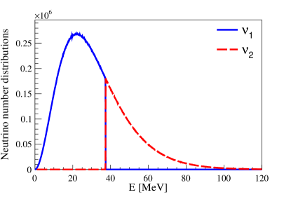
Figure 10: (Color online) Final distributions of neutrinos in the mass basis in the case of inverted mass hierarchy. All other parameters are the same as those in Fig. 9.

IX Antineutrinos

The most convenient way to include antineutrinos into this formalism is by using the doublets

$$\begin{pmatrix}-|\bar{\nu}_{2},\mathbf{p}\rangle\\ |\bar{\nu}_{1},\mathbf{p}\rangle\end{pmatrix}\quad\mbox{and}\quad\begin{pmatrix}-|\bar{\nu}_{x},\mathbf{p}\rangle\\ |\bar{\nu}_{e},\mathbf{p}\rangle\end{pmatrix}$$ (139)

Here $|\bar{\nu}_{a},\mathbf{p}\rangle$ denotes an antineutrino in a mass ($a=1,2$) or flavor ($a=e,x$) eigenstate with momentum $\mathbf{p}$. If we denote the corresponding annihilation operator by $b_{a}(\mathbf{p})$, the isospin operators for this doublet structure are given by

$$\bar{J}^{+}_{{\tiny\mathbf{p}},{\mbox{\tiny mass}}}=-b^{\dagger}_{2}(\mathbf{p})b_{1}(\mathbf{p}),\quad\bar{J}^{-}_{{\tiny\mathbf{p}},{\mbox{\tiny mass}}}=-b^{\dagger}_{1}(\mathbf{p})b_{2}(\mathbf{p})$$

$$\bar{J}^{z}_{{\tiny\mathbf{p}},{\mbox{\tiny mass}}}={\frac{1}{2}}{\big{(}b^{\dagger}_{2}(\mathbf{p})b_{2}(\mathbf{p})-b^{\dagger}_{1}(\mathbf{p})b_{1}(\mathbf{p})\big{)}}$$ (140a)

$$\bar{J}^{+}_{{\tiny\mathbf{p}},{\mbox{\tiny flavor}}}=-b^{\dagger}_{x}(\mathbf{p})b_{e}(\mathbf{p}),\quad\bar{J}^{-}_{{\tiny\mathbf{p}},{\mbox{\tiny flavor}}}=-b^{\dagger}_{e}(\mathbf{p})b_{x}(\mathbf{p})$$

$$\bar{J}^{z}_{{\tiny\mathbf{p}},{\mbox{\tiny flavor}}}={\frac{1}{2}}{\big{(}b^{\dagger}_{x}(\mathbf{p})b_{x}(\mathbf{p})-b^{\dagger}_{e}(\mathbf{p})b_{e}(\mathbf{p})\big{)}}$$ (140b)

in mass and flavor bases respectively. As we did for neutrinos, we drop the “mass” index from the antineutrino mass isospin operators:

$$\bar{J}^{\pm,0}_{{\tiny\mathbf{p}},{\mbox{\tiny mass}}}\to\bar{J}^{\pm,0}_{{\tiny\mathbf{p}}}.$$ (141)

Following the established practice in this field, we define the “energy” as $E=-|\mathbf{p}|$ for antineutrinos. Accordingly their “vacuum oscillation frequencies” $\omega$ defined in Eq. (8) are also allowed to take negative values. Characterizing antineutrinos with the doublet in Eq. (139) and using negative energies helps one to seamlessly integrate them into the formulation (see Refs. Duan et al. (2007a, b), for example). One only needs to keep in mind that the physical values of energy and vacuum oscillation frequency for antineutrinos are equal to $-E$ and $-\omega$, respectively. The summation formula in Eq. (9) generalizes to antineutrinos as

$${\vec{J}_{\omega}}=\sum_{|\mathbf{p}|=-E}{\vec{\bar{J}}_{\mathbf{p}}}$$ (142)

This formula tells us that $\vec{J}_{\omega}$ for $\omega<0$ represents the total isospin of all antineutrinos with energy $E<0$. The formula for the summation over all modes given in Eq. (10) is now generalized to include both positive and negative oscillation frequencies so that $\vec{J}$ represents the total isospin of both neutrinos and antineutrinos. In this case the operator $U$ defined in Eq. (12) transforms both neutrinos and antineutrinos between flavor and mass bases. Finally, the summation convention for other quantities described in Sec. II.2 also generalizes in a similar fashion: $\bar{Q}_{\mathbf{p}}$ and $Q_{\omega<0}$ refer to the antineutrino analogs of the corresponding neutrino quantities, while $Q$ refers to the same quantity summed over all neutrinos and antineutrinos. In particular, $n$ now denotes the total number of neutrinos and antineutrinos in the ensemble.

With these definitions, the many-body Hamiltonian describing neutrinos and antineutrinos which undergo vacuum oscillations and self-interactions is given by

$$H=-\sum_{\omega}\omega J_{\omega}^{z}+\mu\vec{J}\cdot\vec{J}\hskip 0.5pt,$$ (143)

This Hamiltonian has the same form as the one given in Eq. (28) except that now the range of $\omega$ extends to include negative values corresponding to antineutrinos. Because of the reversed definition of isospin doublets for antineutrinos, Eq. (30), describing its analogy with the other many-body systems, is now generalized to

$$\begin{split}&|\uparrow\downarrow\mkern-23.0mu\textrm{---}\rangle\leftrightarrow|\uparrow\rangle\leftrightarrow\begin{cases}-|\bar{\nu}_{2}\rangle&\mbox{ for }\omega<0,\\ |\nu_{1}\rangle&\mbox{ for }\omega>0,\\ \end{cases}\\ &|\textrm{---}\rangle\leftrightarrow|\downarrow\rangle\leftrightarrow\begin{cases}|\bar{\nu}_{1}\rangle&\mbox{ for }\omega<0,\\ |\nu_{2}\rangle&\mbox{ for }\omega>0,\\ \end{cases}\end{split}$$ (144)

Since the form of the Hamiltonian does not change when we include antineutrinos, and since all calculations that we carried out so far depend only on the isospin structure and the corresponding $SU(2)$ commutators, our results can be extended to include antineutrinos in a trivial way. The following procedure achieves this goal:
1. One first shifts the origin of the range of $\omega$ to allow for negative frequencies.
2. Then, for the negative frequencies one needs to substitute

$$\begin{split}\nu_{1}\to-\bar{\nu}_{2},\qquad\nu_{2}\to\bar{\nu}_{1},\\ \end{split}$$ (145)

In connection with the Bethe ansatz formalism, the first step would correspond to shifting the origin of the coordinate system in the electrostatic analogy shown in Fig. 5. Clearly the electrostatic system is invariant under a translation along the $x$ axis, reflecting the invariance of Bethe ansatz equations under a transformation which takes $\omega\to\omega+a$ and $\xi_{\alpha}\to\xi_{\alpha}+a$ where $a$ is a real parameter. Therefore, all the conclusions that we draw from the Bethe ansatz formalism about the many-body eigenstates of the Hamiltonian and how they change as the neutrino self-interactions decrease are still valid.

The substitution in Eq. (145) also leads to

$$\begin{split}\nu_{e}\to-\bar{\nu}_{x},\qquad\nu_{x}\to\bar{\nu}_{e}\end{split}$$ (146)

in agreement with the mixing formula in Eq. (1). In particular, the initial state that we started with in Eq. (102) becomes

$$|\psi\rangle_{\mbox{\tiny initial}}=|\underbrace{\bar{\nu_{x}},\dots,\bar{\nu}_{x}}_{\omega<0},\underbrace{\nu_{e},\dots,\nu_{e}}_{\omega>0}\rangle=|\frac{n}{2},\frac{n}{2}\rangle_{\mbox{\tiny flavor}}$$ (147)

As $\mu$ decreases from very large to very small values under the assumption of perfect adiabaticity, this state evolves to

$$|\psi\rangle_{\mbox{\tiny final}}= \sum_{m=-n/2}^{n/2}(\cos\theta)^{(\frac{n}{2}+m)}(\sin\theta)^{(\frac{n}{2}-m)}$$

$$\times\sqrt{n\choose{\frac{n}{2}+m}}\phi_{m}|\underbrace{\Uparrow,\dots,\Uparrow}_{\frac{n}{2}+m},\underbrace{\Downarrow,\dots,\Downarrow}_{\frac{n}{2}-m}\rangle.$$ (148)

This result is obtained by making the substitution given in Eq. (145) for negative frequencies in Eq. (VII). The states $|\Uparrow\rangle$ and $|\Downarrow\rangle$ refer to the neutrino mass isospin: They are defined as

$$\begin{split}&|\Uparrow\rangle=\begin{cases}-|\bar{\nu}_{2}\rangle&\mbox{ for }\omega<0,\\ |\nu_{1}\rangle&\mbox{ for }\omega>0,\\ \end{cases}\\ &|\Downarrow\rangle=\begin{cases}|\bar{\nu}_{1}\rangle&\mbox{ for }\omega<0,\\ |\nu_{2}\rangle&\mbox{ for }\omega>0.\\ \end{cases}\end{split}$$ (149)

For the final state in Eq. (IX), the normalized energy distribution functions are given by the same formula as in Eq. (115) except that $\omega_{k}$ can now be both positive and negative, and $a$ takes values in $\{\Uparrow,\Downarrow\}$. The $+$ sign in Eq. (115) is for $\Uparrow$ and the $-$ sign is for $\Downarrow$. The value of $m_{\omega_{k}}$ in Eq. (115) can now be found from

$$m_{\omega_{k}}=\begin{cases}\displaystyle{n_{\omega_{k}}/2},&\mbox{for }k<s(m)\\ \displaystyle{\frac{n^{(\Uparrow)}_{\omega_{s(m)}}-n^{(\Downarrow)}_{\omega_{s(m)}}}{2}},&\mbox{for }k=s(m)\\ \displaystyle{-n_{\omega_{k}}/2},&\mbox{for }k>s(m)\\ \end{cases}$$ (150)

with $s(m)$ defined by the same formula as in Eq. (106). With these definitions, Eq. (115) now gives us both neutrino and antineutrino distributions as

$$\begin{split}&\Phi^{(\Uparrow)}(\omega)=\begin{cases}\Phi^{(\bar{\nu}_{2})}(\omega)&\mbox{ for }\omega<0,\\ \Phi^{(\nu_{1})}(\omega)&\mbox{ for }\omega>0,\end{cases}\\ &\Phi^{(\Downarrow)}(\omega)=\begin{cases}\Phi^{(\bar{\nu}_{1})}(\omega)&\mbox{ for }\omega<0,\\ \Phi^{(\nu_{2})}(\omega)&\mbox{ for }\omega>0,\end{cases}\end{split}$$ (151)

in accordance with Eq. (149). Note that the minus sign in Eq. (149) has no consequences in the final energy spectra given in Eq. (151) because they cancel each other when we calculate the expectation values.

In Fig. 11, we show the numerical results for an initial thermal distribution of $\nu_{e}$ and $\bar{\nu}_{x}$ with the respective temperatures of $10$ MeV and $12$ MeV [Fig. 11(a)]. The final energy distributions shown in Fig. 11(b) exhibit a single spectral split in the neutrino sector. This can be easily understood with an analysis similar to the one provided between Eqs. (118) and (122) which leads to the same formula as in Eq. (119) with the mean split frequency $\bar{\omega}_{s}$ given by the formula

$$\int_{-\infty}^{\bar{\omega}_{s}}n_{\omega}\rho_{\omega}d\omega=n\cos^{2}\theta$$ (152)

This formula is the same as what one would derive from the conservation of $\langle J_{z}\rangle$ within the mean field approximation. For the thermal distributions adopted in Eq. (117), it yields $\bar{\omega}_{s}=5.70\times 10^{-3}$ km^-1, which corresponds to $E=33.3$ MeV and agrees with Fig. 11.

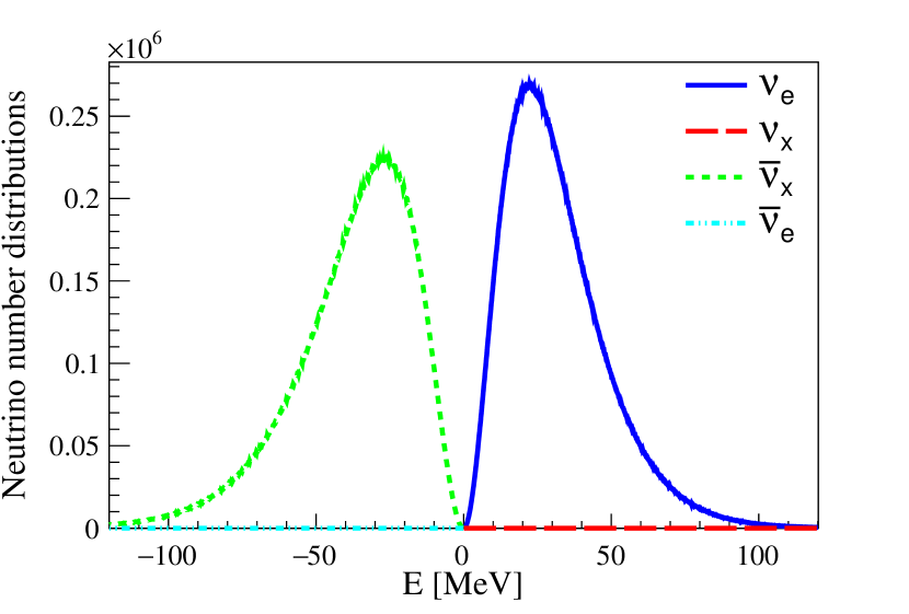
(a) Initial thermal distributions of $\nu_{e}$ and $\bar{\nu}_{x}$.

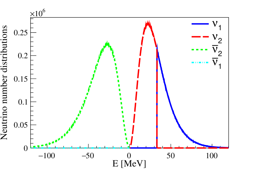
(b) Final distributions in mass basis.

Figure 11: (Color online) Adiabatic evolution of an initial distribution of thermal $\nu_{e}$ and $\bar{\nu}_{x}$. We take the temperature $kT=10$ MeV for neutrinos and $kT=12$ MeV for antineutrinos. We have $10^{8}$ neutrinos occupying $1200$ oscillation modes which are equally spaced in energy. The same is also true for antineutrinos. We adopt the normal mass hierarchy with solar mixing parameters.

X Conclusions

We considered the many-body system formed by neutrinos undergoing vacuum oscillations and self-interactions through neutral current weak force. As is standard in the literature, we represented neutrinos as plane waves in a box so that they all interact with each other at the same time. In the effective two flavor mixing scenario that we work with, this many-body system is analogous to a system of spins with long-range interactions, and to a system of fermions with pairing. We study this neutrino many-body system in the context of a core collapse supernova where it is believed to play an important role with such emergent effects as the spectral splits. However, this current study is not meant to be a comprehensive analysis of many-body effects under the complicated setting of a real supernova. We retain only some of the simple aspects of supernova such as a decreasing self-interaction rate as the neutrinos radiate from the proto-neutron star at the center. A constant matter background can also be incorporated by using matter effective mixing parameters instead of vacuum mixing parameters, although we did not explicitly do this in our numerical calculations.

The focus of our study is the exact many-body behavior of self-interacting neutrinos in comparison to their behavior under the commonly used mean field approximation. The latter formulation reduces the $2^{n}$-dimensional Hilbert space to $n$ individual two-dimensional Hilbert spaces for $n$ neutrinos by omitting the entangled neutrino states. Our technique also involves the reduction of the dimensionality of the Hilbert space, but in a different way. Rather than omitting part of the Hilbert space, we first determined and classified the exact many-body eigenstates of the neutrino Hamiltonian using the Richardson-Gaudin formalism and then identified those eigenstates which project onto our initial state. This strategy allows one to work with a smaller part of the full Hilbert space without any omissions.

Our choice of the initial state in this paper is the simplest one that can be studied with this prescription. It consists of only electron neutrinos (to which antineutrinos of the orthogonal flavor can also be added). It projects only on the highest energy eigenstates of the Hamiltonian for all possible values of the conserved $z$ component of the total mass isospin operator. Those eigenstates do not undergo any level crossings with the other eigenstates, allowing one to easily follow their evolution under the assumption of perfect adiabaticity. We have shown that our initial state adiabatically develops into a superposition of some states, each with a different split point. However, we have shown that those states which significantly contribute to the sum have their split frequencies within $(100/\sqrt{n})\%$ of a mean split frequency. This mean split frequency dominates the final energy distribution, so it is the only apparent pattern in it. The formula for this mean split frequency is the same as what one would obtain with the mean field approximation based on average conservation of the $z$ component of total mass isospin. Therefore, our study demonstrates the validity of the mean field approximation in this particular context in an analytical way.

Although previous studies of the exact many-body dynamics of self-interacting neutrinos have demonstrated the validity of the mean field approximation in their specific settings, this is the first study to include the effects of the vacuum oscillations and the first one to demonstrate the formation of a spectral split which results from an interplay between vacuum oscillation and self-interaction terms. The spectral splits that we obtain in the exact many-body picture are the same as those in the mean field case. In particular, they develop at the same frequency or energy as indicated by Eqs. (121) and (126). As is the case in the mean field formulation, the swap appears in the region which has lower (higher) energy than the split energy in the normal (inverted) mass hierarchy scenarios.

Two important caveats of our study are the lack of a real dynamical evolution and the choice of a particularly simple initial state. Our initial conditions involve no spectral crossings between different neutrino flavors. In that sense, they correspond to the special case examined in Ref. Raffelt and Smirnov (2007b) in the mean field approximation. At present, our formulation does not apply to the splits which arise from instabilities which develop around spectral crossing points, i.e., those discussed in Refs. Dasgupta et al. (2009, 2010); Banerjee et al. (2011). It may be possible to overcome this limitation and apply the formalism to a more general initial condition. This would require a careful examination of the behavior of the system around the points where many-body energy eigenvalues overlap with one another. Self-interacting neutrinos have several dynamical symmetries, and our preliminary studies indicate that the corresponding conservation laws may help us to identify the evolution of a particular many-body energy eigenstate at an energy crossing point. This will be the subject of a future study.

This work was supported in part by TÜBİTAK under Project No. 115F214, in part by the US National Science Foundation Grant No. PHY-1514695, and in part by Grants-in-Aid for Scientific Research of JSPS (No. 15H03665 and No. 17K05459).

Appendix: Energy eigenvalues of bethe ansatz states in strongly interacting regime

In the text we have argued that the Bethe ansatz states with $\kappa$ variables given in Eq. (82) go to the $|j,m\rangle$ states of the total isospin operator given in Eq. (94) in $\mu\to\infty$ limit. In this Appendix, we show that in particular the solution of Bethe ansatz equations in which $k$ of the Bethe ansatz variables remain finite in $\mu\to\infty$ limit while $\kappa-k$ of them go to $-\infty$, produces the eigenstate $|\frac{n}{2}-k,\;-\frac{n}{2}+\kappa\rangle$.

Since the eigenvalue of $J_{z}$ is fixed to $-n/2+\kappa$ by the number of Bethe ansatz variables, we only only need to establish the value of $j$. This can be determined by calculating the energy of the Bethe ansatz state in $\mu\to\infty$ limit and comparing it with Eq. (41).

Since the ordering of the Bethe ansatz variables is not important, we can begin by reordering our variables in such a way that those that approach to $-\infty$ for large $\mu$ are $\xi_{1},\xi_{2},\dotsc,\xi_{\kappa-k}$ and those that stay finite are $\xi_{\kappa-k+1},\dots,\xi_{\kappa}$. Then, the Bethe ansatz equations for the first $p$ variables can be written as follows in $\mu\to\infty$ limit:

$$-\frac{n}{\xi_{\alpha}}=\frac{1}{\mu}-{\sum_{\beta\neq\alpha}^{\kappa}}\frac{2}{\xi_{\alpha}-\xi_{\beta}}$$ (153)

for $\alpha=1,2,\dots,\kappa-k$. Here we ignored the $\omega$ values which are finite valued so that the sum on the left-hand side of Eq. (85) is performed to yield the total number of neutrinos, $n$. The sum on the right-hand side of Eq. (153) can separated into two parts, one running over first $\kappa-k$ (infinite valued) $\xi_{\beta}$’s and the other running over the last $k$ (finite valued) $\xi_{\beta}$’s:

$$\sum_{\beta\neq\alpha}^{\kappa}\frac{2}{\xi_{\alpha}-\xi_{\beta}} = \sum_{\beta(\neq\alpha)=1}^{\kappa-k}\frac{2}{\xi_{\alpha}-\xi_{\beta}}+\sum_{\beta=\kappa-k+1}^{\kappa}\frac{2}{\xi_{\alpha}-\xi_{\beta}}$$ (154)

$$= \frac{2}{\xi_{\alpha}}(k+L_{\alpha})$$

Here $L_{\alpha}$ is given by

$$L_{\alpha}=\sum_{\beta(\neq\alpha)=1}^{p}\frac{\xi_{\alpha}}{\xi_{\alpha}-{\xi_{\beta}}}\hskip 0.5pt.$$ (155)

Substituting it in Eq. (153) we find

$$\xi_{\alpha}=\mu(2L_{\alpha}+2k-n)$$ (156)

Note that, $L_{\alpha}$ depends on $\xi_{\alpha}$ so that Eq. (156) is not an explicit solution. However, this expression is very useful in calculating the energy. By substituting Eq. (156) in Eq. (84), we find the energy of the eigenstate $|\xi_{1},\xi_{2},\dotsc,\xi_{\kappa-k},\xi_{\kappa-k+1},\dots,\xi_{\kappa}\rangle$ as

$$E =E_{-n/2}-\kappa\mu(n-\kappa+1)-\sum_{\alpha=1}^{\kappa-k}\xi_{\alpha}$$ (157)

$$=E_{-n/2}-\mu p(2k-n)+2\mu\sum_{\alpha=1}^{\kappa-k}L_{\alpha}$$

where we ignored the contribution of finite valued Bethe ansatz variables in the energy. By summing both sides of Eq. (155) over $\alpha$ and antisymmetrizing the result, one finds that

$$\sum_{\alpha=1}^{\kappa-k}L_{\alpha}=(\kappa-k)(\kappa-k-1)$$ (158)

Therefore, the energy in Eq. (157) is equal to

$$E=\mu(n/2-k)(n/2-k+1)$$ (159)

This energy is consistent with Eq. (41) with $j=n/2-k$. However, we know that all representations with $j<n/2$ come in multiplicities Therefore Eq. (159) can only tell us that, in $\mu\to\infty$ limit, the state $|\xi_{1},\xi_{2},\dotsc,\xi_{\kappa-k},\xi_{\kappa-k+1},\dots,\xi_{\kappa}\rangle$ approaches to a linear combination of multiple $|n/2-k,-n/2+\kappa\rangle$ states belonging to different representations with the same $j=n/2-k$. On the other hand, those representations with the same $j$ can always be linearly combined to produce another such representation because any linear combination of $|j,m\rangle$ states gives $j(j+1)$ and $m$ under the actions of $\vec{J}\cdot\vec{J}$ and $J_{z}$, respectively. For this reason, we have a degree of freedom in choosing those representations which come with multiplicities when we add several spins or isospins, as long as they are orthogonal to each other. Since the eigenstates of a Hermitian Hamiltonian are also orthogonal to each other, the $j=n/2-k$ representations can be chosen in such a way that the limit of our Bethe ansatz state $|\xi_{1},\xi_{2},\dotsc,\xi_{\kappa-k},\xi_{\kappa-k+1},\dots,\xi_{\kappa}\rangle$ as $\mu\to\infty$ coincides with a particular $|n/2-k,-n/2+\kappa\rangle$ state.

References

- Patrignani et al. (2016) C. Patrignani et al. (Particle Data Group), Chin. Phys. C40, 100001 (2016).
- Burrows (1990) A. Burrows, Ann.Rev.Nucl.Part.Sci. 40, 181 (1990).
- Kotake et al. (2006) K. Kotake, K. Sato, and K. Takahashi, Rept.Prog.Phys. 69, 971 (2006), arXiv:astro-ph/0509456 [astro-ph] .
- Beacom (2010) J. F. Beacom, Ann.Rev.Nucl.Part.Sci. 60, 439 (2010), arXiv:1004.3311 [astro-ph.HE] .
- Raffelt (1996) G. G. Raffelt, Stars as Laboratories for Fundamental Physics (University of Chicago Press, 1996).
- Colgate and White (1966) S. A. Colgate and R. H. White, Astrophys.J. 143, 626 (1966).
- Woosley and Weaver (1986) S. Woosley and T. Weaver, Ann.Rev.Astron.Astrophys. 24, 205 (1986).
- Arnett et al. (1989) W. D. Arnett, J. N. Bahcall, R. P. Kirshner, and S. E. Woosley, Ann. Rev. Astron. Astrophys. 27, 629 (1989).
- Ruffert and Janka (1999) M. Ruffert and H. Janka, Astron.Astrophys. 344, 573 (1999), arXiv:astro-ph/9809280 [astro-ph] .
- Popham et al. (1999) R. Popham, S. Woosley, and C. Fryer, Astrophys.J. 518, 356 (1999), arXiv:astro-ph/9807028 [astro-ph] .
- Narayan et al. (2001) R. Narayan, T. Piran, and P. Kumar, (2001), arXiv:astro-ph/0103360 [astro-ph] .
- Matteo et al. (2002) T. D. Matteo, R. Perna, and R. Narayan, Astrophys.J. 579, 706 (2002), arXiv:astro-ph/0207319 [astro-ph] .
- Chen and Beloborodov (2007) W.-X. Chen and A. M. Beloborodov, Astrophys.J. 657, 383 (2007), arXiv:astro-ph/0607145 [astro-ph] .
- Malkus et al. (2012) A. Malkus, J. Kneller, G. McLaughlin, and R. Surman, Phys.Rev. D86, 085015 (2012), arXiv:1207.6648 [hep-ph] .
- Tian et al. (2017) J. Y. Tian, A. V. Patwardhan, and G. M. Fuller, Phys. Rev. D96, 043001 (2017), arXiv:1703.03039 [astro-ph.HE] .
- Fowler and Hoyle (1964) W. A. Fowler and F. Hoyle, Astrophys.J.Suppl. 9, 201 (1964).
- Barkat (1975) Z. Barkat, Annual Review of Astronomy and Astrophysics 13, 45 (1975).
- Epstein et al. (1988) R. Epstein, S. Colgate, and W. Haxton, Phys.Rev.Lett. 61, 2038 (1988).
- Woosley et al. (1990) S. Woosley, D. Hartmann, R. Hoffman, and W. Haxton, Astrophys.J. 356, 272 (1990).
- Woosley et al. (1994) S. Woosley, J. Wilson, G. Mathews, R. Hoffman, and B. Meyer, Astrophys.J. 433, 229 (1994).
- Woosley et al. (2002) S. Woosley, A. Heger, and T. Weaver, Rev.Mod.Phys. 74, 1015 (2002).
- Totani et al. (1998) T. Totani, K. Sato, H. Dalhed, and J. Wilson, Astrophys.J. 496, 216 (1998), arXiv:astro-ph/9710203 [astro-ph] .
- Katz and Spiering (2012) U. Katz and C. Spiering, Prog.Part.Nucl.Phys. 67, 651 (2012), arXiv:1111.0507 [astro-ph.HE] .
- Scholberg (2012) K. Scholberg, Ann.Rev.Nucl.Part.Sci. 62, 81 (2012), arXiv:1205.6003 [astro-ph.IM] .
- Duan et al. (2010) H. Duan, G. M. Fuller, and Y.-Z. Qian, Ann.Rev.Nucl.Part.Sci. 60, 569 (2010), arXiv:1001.2799 [hep-ph] .
- Chakraborty et al. (2016) S. Chakraborty, R. Hansen, I. Izaguirre, and G. Raffelt, Nucl. Phys. B908, 366 (2016), arXiv:1602.02766 [hep-ph] .
- Samuel (1993) S. Samuel, Phys.Rev. D48, 1462 (1993).
- Raffelt et al. (1993) G. Raffelt, G. Sigl, and L. Stodolsky, Phys. Rev. Lett. 70, 2363 (1993), [Erratum: Phys. Rev. Lett.98,069902(2007)], arXiv:hep-ph/9209276 [hep-ph] .
- Sigl and Raffelt (1993) G. Sigl and G. Raffelt, Nucl.Phys. B406, 423 (1993).
- McKellar and Thomson (1994) B. H. J. McKellar and M. J. Thomson, Phys. Rev. D49, 2710 (1994).
- Gertjerenken and Weiss (2013) B. Gertjerenken and C. Weiss, Phys. Rev. A 88, 033608 (2013), arXiv:1308.5805 [cond-mat.quant-gas] .
- Sørensen et al. (2001) A. Sørensen, L.-M. Duan, J. I. Cirac, and P. Zoller, Nature (London) 409, 63 (2001), quant-ph/0006111 .
- Pezzé and Smerzi (2009) L. Pezzé and A. Smerzi, Physical Review Letters 102, 100401 (2009), arXiv:0711.4840 [quant-ph] .
- Estève et al. (2008) J. Estève, C. Gross, A. Weller, S. Giovanazzi, and M. K. Oberthaler, Nature (London) 455, 1216 (2008), arXiv:0810.0600 .
- Friedland and Lunardini (2003a) A. Friedland and C. Lunardini, Phys.Rev. D68, 013007 (2003a), arXiv:hep-ph/0304055 [hep-ph] .
- Bell et al. (2003) N. F. Bell, A. A. Rawlinson, and R. Sawyer, Phys.Lett. B573, 86 (2003), arXiv:hep-ph/0304082 [hep-ph] .
- Friedland and Lunardini (2003b) A. Friedland and C. Lunardini, JHEP 0310, 043 (2003b), arXiv:hep-ph/0307140 [hep-ph] .
- Duan et al. (2006) H. Duan, G. M. Fuller, J. Carlson, and Y.-Z. Qian, Phys.Rev. D74, 105014 (2006), arXiv:astro-ph/0606616 [astro-ph] .
- Raffelt and Smirnov (2007a) G. G. Raffelt and A. Y. Smirnov, Phys.Rev. D76, 125008 (2007a), arXiv:0709.4641 [hep-ph] .
- Raffelt and Smirnov (2007b) G. G. Raffelt and A. Y. Smirnov, Phys.Rev. D76, 081301 (2007b), [Erratum-ibid. D 77, 029903 (2008)], arXiv:0705.1830 [hep-ph] .
- Pehlivan et al. (2011) Y. Pehlivan, A. Balantekin, T. Kajino, and T. Yoshida, Phys.Rev. D84, 065008 (2011), arXiv:1105.1182 [astro-ph.CO] .
- Raffelt (2011) G. G. Raffelt, Phys.Rev. D83, 105022 (2011), arXiv:1103.2891 [hep-ph] .
- Galais and Volpe (2011) S. Galais and C. Volpe, Phys. Rev. D84, 085005 (2011), arXiv:1103.5302 [astro-ph.SR] .
- Bethe (1931) H. A. Bethe, Z. Phys. 71, 205 (1931).
- Richardson (1963) R. W. Richardson, Physics Letters 3, 277 (1963).
- Gaudin (1976) M. Gaudin, J. Physique 37, 1087 (1976).
- Gaudin (1983) M. Gaudin, La fonction d’onde de Bethe (Collection du Commissariat a l’energie atomique) (Masson, 1983).
- Dukelsky et al. (2004) J. Dukelsky, S. Pittel, and G. Sierra, Rev.Mod.Phys. 76, 643 (2004), arXiv:nucl-th/0405011 [nucl-th] .
- Faribault et al. (2011) A. Faribault, O. E. Araby, C. Strater, and V. Gritsev, Phys.Rev. B83, 235124 (2011), arXiv:1103.0472 [cond-mat.mes-hall] .
- Torrontegui et al. (2013) E. Torrontegui, S. Ibáñez, S. Martínez-Garaot, M. Modugno, A. del Campo, D. Guéry-Odelin, A. Ruschhaupt, X. Chen, and J. G. Muga, Advances in Atomic Molecular and Optical Physics 62, 117 (2013), arXiv:1212.6343 [quant-ph] .
- Balantekin and Pehlivan (2007) A. Balantekin and Y. Pehlivan, J.Phys. G34, 47 (2007), arXiv:astro-ph/0607527 [astro-ph] .
- Volpe et al. (2013) C. Volpe, D. Väänänen, and C. Espinoza, Phys.Rev. D87, 113010 (2013), arXiv:1302.2374 [hep-ph] .
- Volpe (2015) C. Volpe, Int. J. Mod. Phys. E24, 1541009 (2015), arXiv:1506.06222 [astro-ph.SR] .
- Bogoliubov (1946) N. Bogoliubov, Journal of Physics USSR 10, 265 (1946).
- Born and Green (1946) M. Born and H. S. Green, Proc. Roy. Soc. Lond. A188, 10 (1946).
- Kirkwood (1935) J. G. Kirkwood, J.Chem.Phys. 3, 300 (1935).
- Yvon (1935) J. Yvon, La théorie statistique des fluides et l’équation d’état, Actualités scientifiques et industrielles, Vol. 203 (Hermann & cie (Paris), 1935).
- de Gouvea and Shalgar (2012) A. de Gouvea and S. Shalgar, JCAP 1210, 027 (2012), arXiv:1207.0516 [astro-ph.HE] .
- de Gouvea and Shalgar (2013) A. de Gouvea and S. Shalgar, JCAP 1304, 018 (2013), arXiv:1301.5637 [astro-ph.HE] .
- Pehlivan et al. (2014) Y. Pehlivan, A. Balantekin, and T. Kajino, Phys.Rev. D90, 065011 (2014), arXiv:1406.5489 [hep-ph] .
- Serreau and Volpe (2014) J. Serreau and C. Volpe, Phys.Rev. D90, 125040 (2014), arXiv:1409.3591 [hep-ph] .
- Wolfenstein (1978) L. Wolfenstein, Phys.Rev. D17, 2369 (1978).
- Barger et al. (1980) V. Barger, K. Whisnant, S. Pakvasa, and R. J. N. Phillips, Phys. Rev. D 22, 2718 (1980).
- Langacker et al. (1983) P. Langacker, J. P. Leveille, and J. Sheiman, Phys. Rev. D 27, 1228 (1983).
- Kuo and Pantaleone (1989) T.-K. Kuo and J. T. Pantaleone, Rev.Mod.Phys. 61, 937 (1989).
- Janka et al. (2007) H.-T. Janka, K. Langanke, A. Marek, G. Martinez-Pinedo, and B. Mueller, Phys.Rept. 442, 38 (2007), arXiv:astro-ph/0612072 [astro-ph] .
- Pantaleone (1992a) J. T. Pantaleone, Phys.Lett. B287, 128 (1992a).
- Pantaleone (1992b) J. T. Pantaleone, Phys.Rev. D46, 510 (1992b).
- Sawyer (2005) R. Sawyer, Phys.Rev. D72, 045003 (2005), arXiv:hep-ph/0503013 [hep-ph] .
- Roberts and Reddy (2016) L. F. Roberts and S. Reddy, (2016), arXiv:1612.03860 [astro-ph.HE] .
- Duan and Friedland (2011) H. Duan and A. Friedland, Phys. Rev. Lett. 106, 091101 (2011), arXiv:1006.2359 [hep-ph] .
- Bardeen et al. (1957) J. Bardeen, L. Cooper, and J. Schrieffer, Phys.Rev. 108, 1175 (1957).
- Mayer (1950a) M. G. Mayer, Physical Review 78, 16 (1950a).
- Mayer (1950b) M. G. Mayer, Physical Review 78, 22 (1950b).
- Bloch et al. (2008) I. Bloch, J. Dalibard, and W. Zwerger, Rev. Mod. Phys. 80, 885 (2008).
- Giorgini et al. (2008) S. Giorgini, L. P. Pitaevskii, and S. Stringari, Rev. Mod. Phys. 80, 1215 (2008).
- Randeria and Taylor (2014) M. Randeria and E. Taylor, Ann. Rev. Condensed Matter Phys. 5, 209 (2014), arXiv:1306.5785 [cond-mat.quant-gas] .
- Inouye et al. (1998) S. Inouye, M. R. Andrews, J. Stenger, H.-J. Miesner, D. M. Stamper-Kurn, and W. Ketterle, Nature 392, 151 (1998).
- Richardson and Sherman (1964) R. Richardson and N. Sherman, Nuclear Physics 52, 253 (1964).
- Richardson (1966) R. Richardson, Phys.Rev. 141, 949 (1966).
- Cambiaggio et al. (1997) M. C. Cambiaggio, A. M. F. Rivas, and M. Saraceno, Nucl. Phys. A624, 157 (1997), arXiv:nucl-th/9708031 [nucl-th] .
- Pehlivan et al. (2017) Y. Pehlivan, A. L. Subaşı, N. Ghazanfari, S. Birol, and H. Yüksel, Phys. Rev. D95, 063022 (2017), arXiv:1603.06360 [astro-ph.HE] .
- Zwierlein et al. (2004) M. W. Zwierlein, C. A. Stan, C. H. Schunck, S. M. F. Raupach, A. J. Kerman, and W. Ketterle, Phys. Rev. Lett. 92, 120403 (2004).
- Gaudin (1968) M. Gaudin, États propres et valeurs propres de l’Hamiltonien d’appariement, (1968) unpublished. Saclay preprint. Included in: Travaux de M. Gaudin, Modèles Exactement Résolus (Les Èditions de Physique), 1995.
- Richardson (1977) R. W. Richardson, Journal of Mathematical Physics 18, 1802 (1977).
- Ismail (2000) M. E. Ismail, Numerical Functional Analysis and Optimization 21, 191 (2000).
- McMillen et al. (2009) T. McMillen, A. Bourget, and A. Agnew, Journal of Computational and Applied Mathematics 223, 862 (2009).
- Pogosov and Combescot (2011) W. V. Pogosov and M. Combescot, Physica C Superconductivity 471, 566 (2011), arXiv:1103.1147 [cond-mat.supr-con] .
- Zhou et al. (2002) H.-Q. Zhou, J. Links, R. H. McKenzie, and M. D. Gould, Phys. Rev. B 65, 060502 (2002).
- Roman et al. (2002) J. Roman, G. Sierra, and J. Dukelsky, Nucl.Phys. B634, 483 (2002), arXiv:cond-mat/0202070 [cond-mat] .
- Dasgupta et al. (2009) B. Dasgupta, A. Dighe, G. G. Raffelt, and A. Yu. Smirnov, Phys. Rev. Lett. 103, 051105 (2009), arXiv:0904.3542 [hep-ph] .
- Dasgupta et al. (2010) B. Dasgupta, A. Mirizzi, I. Tamborra, and R. Tomas, Phys. Rev. D81, 093008 (2010), arXiv:1002.2943 [hep-ph] .
- Banerjee et al. (2011) A. Banerjee, A. Dighe, and G. Raffelt, Phys. Rev. D84, 053013 (2011), arXiv:1107.2308 [hep-ph] .
- Duan et al. (2007a) H. Duan, G. M. Fuller, and Y.-Z. Qian, Phys. Rev. D76, 085013 (2007a), arXiv:0706.4293 [astro-ph] .
- Duan et al. (2007b) H. Duan, G. M. Fuller, J. Carlson, and Y.-Z. Qian, Phys. Rev. Lett. 99, 241802 (2007b), arXiv:0707.0290 [astro-ph] .