Multi-Meson Model for the $D^{+}\to K^{+}K^{-}K^{+}$ decay amplitude

Abstract

We propose a novel approach to describe the $D^{+}\to K^{-}K^{+}K^{+}$ decay amplitude, based on chiral effective Lagrangians, which can be used to extract information about $K\bar{K}$ scattering. Our trial function is an alternative to the widely used isobar model and includes both nonresonant three-body interactions and two-body rescattering amplitudes, based on coupled channels and resonances, for S- and P-waves with isospin $0$ and $1$. The latter are unitarized in the $K$-matrix approximation and represent the only source of complex phases in the problem. Free parameters are just resonance masses and coupling constants, with transparent physical meanings. The nonresonant component, given by chiral symmetry as a real polynomium, is an important prediction of the model, which goes beyond the (2+1) approximation. Our approach allows one to disentangle the two-body scalar contributions with different isospins, associated with the $f_{0}(980)$ and $a_{0}(980)$ channels. We show how the $K\bar{K}$ amplitude can be obtained from the decay $D^{+}\to K^{-}K^{+}K^{+}$ and discuss extensions to other three-body final states.

I introduction

Nonleptonic weak decays of heavy-flavoured mesons are extensively used in light meson spectroscopy. Owing to a rich resonant structure, these decays provide a natural place to study hadron-hadron interactions at low energies. In particular, almost 20 years ago, three-body decays of charmed mesons could confirm the existence of the controversial scalar states $f_{0}(600)$ (or sigma)sigma and kappa$(800)$E791kappa . More comprehensive investigations can be done nowadays, using the very large and pure samples provided by the LHC experiments, and still more data is expected in the near future, with Belle II experiments.

Three-body hadronic decays of heavy-flavoured mesons involve combinations of different classes of processes, namely heavy-quark weak transitions, hadron formation and final-state interactions (FSI), whereby the hadrons produced in the primary vertex are allowed to interact in many different ways before being detected. Final-state processes include both proper three-body interactions and a wide range elastic and inelastic coupled channels, involving resonances. In this framework, a question arises, concerning how to obtain information about two-body scattering amplitudes from the abundant data on three-body systems.

The key issue of this program is the modeling of the decay amplitudes. Most amplitude analyses have been performed using the so-called isobar model, in which the decay amplitude is represented by a coherent sum of both nonresonant and resonant contributions. This approach, albeit largely employed LHCb_BW_exemplo , has conceptual limitations. The outcome of isobar model analyses are resonance parameters such as fit fractions, masses and widths, which are neither directly related to any underlying dynamical theory nor provide clues to the identification of two-body substructures. Thus, the systematic interpretation of the isobar model results is rather difficult.

This situation motivated in the past decade efforts towards building models that are based on more solid theoretical grounds. Those models improve essentially the two-meson interaction description in the FSI, with the use of dispersion relations and chiral perturbation theory. Most of them work in the quasi-two-body (2+1) approximation, where interactions with the third particle are neglected. Recently, a collection of parametrizations based on analytic and unitary meson-meson form factors for D and B three-body hadronic decays within the (2+1) approximation was presented in Ref.BoitoRESUM . Three-body FSIs were also considered and, in particular, shown to play a significant role in the $D^{+}\rightarrow K^{-}\pi^{+}\pi^{+}$ decay. In this process, three-body unitarity was implemented in different ways, by means of Faddeev-like decompositionsBR ; PatWV ; tobias , Khuri-Treiman equationkubis or triangle diagrams satoshi . Whilst differing in methods and techniques, all these theoretical efforts have in common the attempt to include, in a systematic way, knowledge of two-body systems in the description of the decay amplitudes.

This work departs from the same broad perspective, but concentrates explicitly on the derivation of two-body scattering amplitudes from three-body decays. In order to do so, we suggest a new approach based on effective Lagrangians and apply it to the $D^{+}\to K^{-}K^{+}K^{+}$ decay. This process is interesting because there is very little information available on kaon-kaon scattering, regarding both theory and experiment. Concerning the latter, one only has access to $\pi\pi$ elastic scattering data Hyams and to the inelastic channel $\pi\pi\to K\bar{K}$Hyams ; cohen . Information about $K\bar{K}$ interaction can be estimated by imposing unitarity constraints on the $\pi\pi$ data. On the theory side, $K\bar{K}$ amplitudes have been calculated in next-to-leading order chiral perturbation theory. Aiming at a full coupled-channel description, it was extended up to 1.2 GeV, using form factors mousallam_KKff to describe the $\eta\pi\to K\bar{K}$ contribution to $\eta\to\pi\pi\pi$ decaymousallam_eta3pi , or unitarized ressummation techniquesOllerMeissner , to include $\pi\pi\to K\bar{K}$ in the context of FSI of $J/\Psi\to\phi\pi\pi(K\bar{K})$ decays.

The main purpose of this work is disclose information about the dynamics of $K\bar{K}$ interactions by disentangling the two-body contributions contained in the $D^{+}\to K^{-}K^{+}K^{+}$ amplitude. In our model, the description of the $K\bar{K}$ interaction relies on a chiral Lagrangian with resonances, including all possible coupled channels for ($J=0,1;I=0,1$), extended to non-perturbative regimes by means of unitarization. A relevant feature of the model is that the relative contribution and phase of each component is fixed by theory, and this represents an important difference with the isobar model. Although the formalism is developed for a specific process it can be useful in other decays into three kaons.

This paper extends and supersedes a previous versionTM and is organized as follows. The motivation for building the amplitude is discussed in section II, whereas the model is presented in sections III and IV. The suggested amplitude for data fitting, together with a comparison between scattering and decay amplitudes is discussed in section V. Some simulations and general remarks are given in section VI. Details of the calculations are given in the appendices.

II motivation for a new model

The isobar model, widely used for describing heavy-meson decays into three pseudoscalars, relies on the assumption that these processes are dominated by intermediate states involving a spectator plus a resonance, and also includes non-resonant contributions. In the decay $H\rightarrow P_{1}P_{2}P_{3}$, of a heavy meson $H$ into three pseudoscalars $P_{i}$, the isobar model emphasizes the sequence $H\rightarrow R\,P_{3}$, followed by $R\rightarrow P_{1}P_{2}$.

The full $H\rightarrow P_{1}P_{2}P_{3}$ decay amplitude is denoted by $T$ and the isobar model employs a guess function to be fitted to data in the form of the coherent sum

$${T}=c_{nr}\;\tau_{nr}+\sum c_{k}\;\tau_{k}\;,$$ (1)

the subscript $nr$ referring to the non-resonant term and the label $k$ associated with resonances, as many of them as needed. The coefficients $c_{k}=e^{i\theta_{k}}$ are complex parameters, to be determined by data. The choice $\tau_{nr}=1$ is usual for the non-resonant term, whereas the sub amplitudes $\tau_{k}$ depend on the invariant masses of the problem. For each resonance considered, the function $\tau_{k}$ is given by $\tau_{k}=[FF]\times[\,\mathrm{angular}\;\mathrm{factor}\,]\times[\mathrm{line}\;\mathrm{shape}]_{k}$, where ${FF}$ stands for form factors, the angular factor is associated with angular momentum channels, and $[\mathrm{line}\;\mathrm{shape}]_{k}$ represents a resonance line shape, described by either a Breit-Wigner function such as $(BW)_{k}=1/[s-m_{k}^{2}+i\,m_{k}\,\Gamma_{k}]$, $m_{k}$ and $\Gamma_{k}$ being the resonance mass and width, or by variations, such as the Flatté or Gounaris-Sakurai forms. The angular factor allows one to distinguish partial wave contributions and to employ the decomposition $T=T^{S}+T^{P}+\cdots$.

A good fit to decay data based on the structure given by eq.(1), would yield an empirical set of complex parameters $c_{nr}$ and $c_{k}$. However, a question arises regarding the meaning of these parameters. Would they be useful to shed light into yet unknown two-body substructures of the problem? Can they provide reliable information about scattering amplitudes? If we denote two-body scattering amplitudes by $A$ this question may be restated as: can one extract $A$ directly from $T\,$? As we argue in the sequence, answers to these questions do not favour the isobar model.

On general grounds, there is no direct connection between a heavy-meson decay amplitude $T$ and two-body scattering amplitudes $A$, involving the same particles. Their relationship involves several issues, which we discuss below.
a. dynamics - The dynamical contents of $T$ and $A$ are rather different, since the former must include weak vertices, which cannot be present in the latter. Specific features of $W$-meson interactions are important to $T$ and irrelevant to $A$. Therefore, although scattering amplitudes $A$ may be substructures of $T$, there is no reason whatsoever for assuming that these $A$’s are either identical or proportional to $T$. This is supported by case studies. For instance, some time ago, the FOCUS collaborationFOCUS produced a partial-wave analysis of the $S$-wave $K^{-}\pi^{+}$ amplitude from the decay $D^{+}\rightarrow K^{-}\pi^{+}\pi^{+}$. Several groups then compared compare the phase of this empirical amplitude directly with that from the LASS $K^{-}\pi^{+}$ scattering dataLASS and the discrepancy found was seen as a puzzle. The fact that the FOCUS phase was negative at low energies was considered to be especially odd. In the language of this discussion, this kind of puzzle arose just because one was trying to compare $T$ and $A$ directly. The difference between observed $S$-wave decay and scattering phases was later explained by considering meson loops in the weak sector of the problemBR ; PatWV . These loops account for the extra phases observed.
b. good quantum numbers: - Isospin is broken by weak interactions and is a good quantum number for $A$, but not for $T$. Scattering amplitudes $A$ depend both on the angular momentum $J$ and on the isospin $I$ of the channel considered, whereas just a $J$ dependence can be extracted from an empirical decay amplitude $T$. This point will be recast on more technical grounds while we discuss our model. For the time being, it suffices to stress that it is impossible to derive directly $A^{(J,I)}$ from $T^{(J)}$ simply because the former contains more structure than the latter. An extraction of $A^{(J,I)}$ from $T^{(J)}$ would amount to generating physical content about the isospin structure.
c. coupled channels - It is well known that scattering amplitudes include important inelasticities due to couplings of intermediate states. For instance, as Hyams et al.Hyams point out, $K\bar{K}$ intermediate states do influence elastic $\pi\pi$ scattering at some energies. Since scattering amplitudes $A$ are substructures of the decay amplitude $T$, coupled channels present in the former must also show up in the latter. In general, guess functions better suited for accommodating data should have structures similar to those used in meson-meson scattering Refs.Hyams ; mousallam_KKff ; Pelaez . In the case of the isobar model, the simple guess functions usually employed fail to incorporate these intermediate couplings.
d. unitarity - Good fits to Dalitz plots data may require several resonances with the same quantum numbers. At present, conceptual techniques are available which preserve unitarity while incorporating several resonances into amplitudesOOunit . This allows one to go beyond the isobar model, where the amplitude is constructed as sums of individual line shapes (Breit-Wigner), as in eq.(1), a procedure known to violate unitarity, even in the case of scattering amplitudesunit .
e. non-resonant term - The non-resonant term may be important and involve less known interactions. In the case of heavy meson decays and some leptonic reactions, available energies can be large enough for allowing the simultaneous production of several pseudoscalars at a single vertex. Multi-meson dynamics then becomes relevant. For instance, the process $e^{-}\,e^{+}\rightarrow 4\,\pi$ involves the matrix element $\langle\pi\pi\pi\pi|J_{\gamma}^{\mu}|0\rangle$, $J_{\gamma}^{\mu}$ being the electromagnetic currentEU . A similar matrix element, with $J_{\gamma}^{\mu}$ replaced with the weak current $(V\!-\!A)^{\mu}$, describes the decay $\tau\rightarrow\nu\,4\pi$EU . Interactions of this kind are also present in the model for $D^{+}\to K^{-}K^{+}K^{+}$ we discuss here.
f. lagrangians - Although the point of departure of the isobar model may be sound, the problems mentioned tend to corrode the physical meaning of parameters it yields from fits. Thus, even if these fits are precise, the relevance of the parameters extracted remains restricted to specific processes. Moreover, in particular, one cannot rely on them for obtaining scattering information. The most conservative way of ensuring that the physical meaning of parameters is preserved from process to process is to employ lagrangians, which rely on just masses and coupling constants. Guess functions for heavy-meson decays constructed from lagrangians yield free parameters which allow the straightforward derivation of scattering amplitudes.

III dynamics

The fundamental QCD lagrangian for strong interactions is written in terms of gluons and quarks, the basic degrees of freedom. As the theory allows for gluon self-interactions, perturbative calculations hold at high energies only. At present, intermediate-energy reactions cannot be described in terms of quarks and gluons, and one is forced to rely on effective theories. At low energies, chiral perturbation theory (ChPT) WChPT ; GL84 ; GL85 is highly successful. It is ideally suited for describing interactions of pseudoscalar mesons in the $SU(3)$ flavour sector, but can also encompass baryons. A prominent feature of ChPT is that it realizes the hidden symmetry of the QCD ground state, that manifests itself as a vacuum filled with $u\bar{u},d\bar{d}$, and $s\bar{s}$ states. The lowest energy excitations of this vacuum are the pseudoscalar mesons, which are highly collective states. Another remarkable feature of the theory is that it yields multi-meson contact interactions. For instance, depending on the energy, reactions such as $\pi\pi\rightarrow\pi\pi K\bar{K}$ may involve a single interaction. On a more technical side, in ChPT, amplitudes are systematically expanded in terms of polynomials, involving both kinematical variables and quark masses. The orders of these polynomials, assessed at a scale $\Lambda\sim 1$ GeV, determine a dynamical hierarchy and leading order (LO) contributions correspond to multi-meson contact interactions, whereas resonance exchanges are next-to-leading order (NLO). This understanding motivated an extension of the original chiral perturbation theory formalism, known as (ChPTR), in which resonances are explicitly included EGPR . At present, ChPT yields the most reliable representation of the Standard Model at low energies.

Low-energy applications of ChPT are normally restricted to regions below the $\rho$ mass whereas, in $D$ decays, energies above $1.5\,$GeV are involved. Therefore, the description of hadronic interactions at those higher energies requires further extensions of the theory, which must include non-perturbative effects in a controlled way. A widely used and rather successful approach consists in ressumming a Dyson series based on chiral interactions, so as to obtain unitary scattering amplitudesOOunit . In this work, we deal with the process $D^{+}\to K^{-}K^{+}K^{+}$ and, in principle, it should be described by a properly unitarized three-body amplitude. However, this is beyond present possibilities and, following the usual practice, we work in the so called $(2\!+\!1)$ approximation, in which two-body unitarized amplitudes are coupled to spectator particles. Throughout the paper, we use the notation and conventions of Ref.EGPR . If needed, another extension scheme for ChPT, based on the explicit inclusion of heavy mesonsHM , is also available.

The theoretical description of a heavy meson decay into pseudoscalars involve two quite distinct sets of interactions. The first one concerns the primary weak vertex, in which a heavy quark, either $c$ or $b$, emits a $W$ and becomes a $SU(3)$ quark. As this process occurs inside the heavy meson, it corresponds to the effective decay of a $D$ or a $B$ into a first set of $SU(3)$ mesons. ChPT is fully suited for describing these effective processes. The primary weak decay is then followed by purely hadronic final state interactions (FSIs), in which the mesons produced initially rescatter in many different ways, before being detected. The decay $D^{+}\to K^{-}K^{+}K^{+}$ is doubly-Cabibbo-suppressed and any model describing it should involve a combination of these two parts, as suggested by Fig.1.

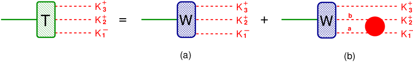
Figure 1: Amplitude $T$ for $D^{+}\rightarrow K^{-}\,K^{+}\,K^{+}$: (a) primary weak vertex; (b) weak vertex dressed by final state interactions; the full line is the $D$, dashed lines are pseudoscalars.

In this work we allow for the coupling of intermediate states and, within the $(2+1)$ approximation, final state interactions are always associated with loops describing two-meson propagators. This provides a topological criterion for distinguishing the primary weak vertex from FSIs, namely that the former is represented by tree diagrams and the latter by a series with any number of loops. Each of these loops is multiplied by a tree-level scattering amplitude ${\cal{K}}$ and, schematically, this allows the decay amplitude $T$ to be written as

$$T=(\mathrm{weak\;tree})\,\times\,\left[1+(\mathrm{loop}\times{\cal{K}})+(\mathrm{loop}\times{\cal{K}})^{2}+(\mathrm{loop}\times{\cal{K}})^{3}+\cdots\right]\,.$$ (2)

The term within square brackets involves strong interactions only and represents a geometric series for the FSIs, which can be summed. Denoting this sum by $S$, one has $S=1/[1-(\mathrm{loop}\times{\cal{K}})]$, which corresponds to the model prediction for the resonance line shape.

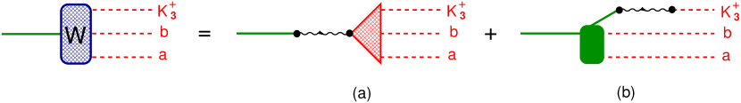
Figure 2: Competing topologies for the decay $D^{+}\rightarrow K^{-}\,K^{+}\,K^{+}$;as the pair $P^{a}P^{b}$ is produced either after (a) or before (b) the weak interaction.

The weak amplitude describes the process $D\rightarrow(P^{a}P^{b})K^{+}$ at tree level, where $P^{i}$ corresponds to a pseudoscalar with $SU(3)$ label $i$. There are two competing topologies representing it, given by Fig.2. A peculiar feature of these vertices is that process (a) can yield $P^{a}P^{b}=K^{-}K^{+}$, whereas process (b) cannot. This can be seen by inspecting the quark structure of the latter, given in Fig.3, which shows that just a $d\bar{d}$ pair is available as a source of the two outgoing mesons at the strong vertex. Hence one could have $P^{a}P^{b}=\pi^{0}\pi^{0},\pi^{+}\pi^{-},K^{0}\bar{K}^{0}$, but not $P^{a}P^{b}=K^{-}K^{+}$. The production of a $K^{-}K^{+}$ final state by mechanism (b) would thus require at least one FSI. In terms of the scheme depicted in eq.(2), this means that the first factor within the square bracket would be absent and the decay amplitude could be rewritten as

$$T=(\mathrm{weak\;tree})\,\times\,(\mathrm{loop}\times{\cal{K}})\times\left[1+(\mathrm{loop}\times{\cal{K}})+(\mathrm{loop}\times{\cal{K}})^{2}+(\mathrm{loop}\times{\cal{K}})^{3}+\cdots\right]\,.$$ (3)

Mechanism (b) is therefore suppressed when compared with mechanism (a). The Multi-Meson-Model (Triple-M) for the $D^{+}\to K^{-}K^{+}K^{+}$ amplitude proposed here assumes the dominance of process (a) of Fig.2, whereby the decay proceeds through the steps $D^{+}\to W^{+}\to K^{+}K^{-}K^{+}$.

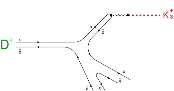
Figure 3: Quark content of topology (b) of Fig.2.

IV multi-meson-model for $D^{+}\to K^{-}K^{+}K^{+}$

Our model is based on the assumption that the weak sector of the doubly-Cabibbo-suppressed decay $D^{+}\rightarrow K^{-}K^{+}K^{+}$ is dominated by the process shown in Fig.2 (a), in which quarks $c$ and $\bar{d}$ in the $D^{+}$ annihilate into a $W^{+}$, which subsequently hadronizes. The primary weak decay is followed by final state interactions, involving the scattering amplitude $A$. This yields the decay amplitude $T$ given in Fig.4, which includes the weak vertex and indicates that the relationship with $A$ is not straightforward.

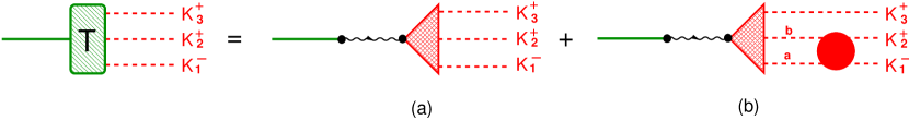
Figure 4: Decay amplitude for $D^{+}\rightarrow K^{-}\,K^{+}\,K^{+}$; the weak vertex proceeds thought the intermediate steps $D^{+}\rightarrow W^{+}$ and $W^{+}\rightarrow K^{-}\,K^{+}\,K^{+}$ and strong final state interactions are encompassed by the scattering amplitude $A$ (full red blob).

This decay amplitude is given by

$$T=-\left[\frac{G_{F}}{\sqrt{2}}\,\sin^{2}\theta_{C}\right]\,\langle K^{-}(p_{1})\,K^{+}(p_{2})\,K^{+}(p_{3})|A^{\mu}|\,0\,\rangle\;\langle\,0\,|A_{\mu}|\,D^{+}(P)\rangle\;,$$ (4)

where $G_{F}$ is the Fermi decay constant, $\theta_{C}$ is the Cabibbo angle, the $A^{\mu}$ are axial currents and $P=p_{1}+p_{2}+p_{3}\,$. Throughout the paper, the label 1 refers to the $K^{-}$, the label 3 the spectator $K^{+}$ and kinematical relations are given in appendix A.

Denoting the $D^{+}$ decay constant by $F_{D}$, we write $\langle\,0\,|A_{\mu}|\,D^{+}(P)\rangle=-i\,\sqrt{2}\,F_{D}\,P_{\mu}$ and find a decay amplitude proportional to the divergence of the remaining axial current, given by

$$T \!=\! i\,\left[\frac{G_{F}}{\sqrt{2}}\,\sin^{2}\theta_{C}\right]\,\sqrt{2}\,F_{D}\;\left[P_{\mu}\,\langle A^{\mu}\rangle\right]\;,$$ (5)

with $\langle A^{\mu}\rangle=\langle K^{-}(p_{1})\,K^{+}(p_{2})\,K^{+}(p_{3})|A^{\mu}|\,0\,\rangle$. This result is important because, if $SU(3)$ were an exact symmetry, the axial current would be conserved and the amplitude $T$ would vanish. As the symmetry is broken by the meson masses, one has the partial conservation of the axial current (PCAC) and $T$ must be proportional to $M_{K}^{2}$. In the expressions below, this becomes a signature of the correct implementation of the symmetry.

Figure 5: Dynamical structure of triangle vertices in Fig.4; the wavy line is the $W^{+}$, dashed lines are mesons, continuous lines are resonances and the full red blob represent meson-meson scattering amplitudes, described in Fig.6; all diagrams within square brackets should be symmetrized, by making $2\leftrightarrow 3$.

The rich dynamics of the decay amplitude $T$ is incorporated in the current $\langle A^{\mu}\rangle$ and displayed in Fig.5. Diagrams are evaluated using the techniques described in Refs.GL85 ; EGPR . In chiral perturbation theory, the primary couplings of the $W^{+}$ to the $K^{-}K^{+}K^{+}$ system always involve a direct interaction, accompanied by a kaon-pole term, denoted by (A) and (B) in the figure. Only their joint contribution is compatible with PCAC. Diagrams (1A+1B) are LO and describe a non-resonant term, a proper three body interaction, which goes beyond the $(2+1)$ approximation, whereas Figs. (2A+2B) allow for the possibility that two of the mesons rescatter, after being produced in the primary weak vertex. Diagrams (3A+3B) are NLO and describe the production of bare resonances at the weak vertex, whereas final state rescattering processes (4A+4B) endow them with widths.

IV.1 two-body unitarization and resonance line shapes

In the description of the two-body subsystem, we consider just $S$- and $P$- waves, corresponding to $(J=1,0,I=1,0)$ spin-isospin channels. The associated resonances are $\rho(770)$, $\phi(1020)$, $a_{0}(980)$, and two $SU(3)$ scalar-isoscalar states, $S_{1}$ and $S_{o}$, corresponding to a singlet and to a member of an octet, respectively. The physical $f_{0}(980)$, together with a higher mass $f_{0}$ state, would be linear combinations of $S_{1}$ and $S_{o}$. Depending on the channel, the intermediate two-meson propagators may involve $\pi\pi$, $KK$, $\eta\eta$, and $\pi\eta$ intermediate states, so there is a large number of coupled channels to be considered.

Figure 6: (a) Tree-level two-body interaction kernel ${\cal{K}}_{ab\rightarrow cd}^{(J,I)}$ - a NLO $s$-channel resonance, added to a LO contact term. (b) Structure of the unitarized scattering amplitude.

The basic meson-meson intermediate interactions $P^{a}P^{b}\rightarrow P^{c}P^{d}$ are described by kernels ${\cal{K}}_{ab|cd}^{(J,I)}$ and their simple dynamical structure is shown in Fig.6, as LO four point terms, typical of chiral symmetry, supplemented by NLO resonance exchanges in the $s$-channel. Just in the $(J=0,I=0)$ channel two resonances, $S_{1}$ and $S_{o}$, are needed. In these diagrams, all vertices represent interactions derived from chiral lagrangiansEGPR . Kernels are then functions depending on just masses and coupling constants. The mathematical structure of these functions is displayed in App.F. In the case of the $\phi$-meson, the kernel includes an effective coupling to the $(\rho\pi+\pi\pi\pi)$ channel, which accounts for about $15\%$ of its width. This effective interaction is discussed in App.(C) and yields eq.(108).

All other resonance terms in the kernels contain bare poles. However, the evaluation of amplitudes involves the iteration of the basic kernels by means of two-meson propagators, as in Fig.6(b). The propagators, denoted by $\bar{\Omega}$, are discussed in App.B and, in principle, have both real and imaginary components. The former contain divergent contributions and their regularization brings unknown parameters into the problem. This considerable nuisance is avoided by working in the $K$-matrix approximation, whereby just the imaginary parts of the two-meson propagators are kept. This gives rise to the structure sketched within the square bracket of eq.(2), where the terms $(\mathrm{loop}\times{\cal{K}})$ are realized by the functions $M_{ij}^{(J,I)}$ given in eqs.(129-132). The ressummation of the geometric series, indicated in Fig.6(b), endows the $s$-channel resonances with widths. Thus among other structures, intermediate two-body amplitudes yield denominators $D^{(J,I)}$, which are akin to those of the form $D_{BW}=[s-m^{2}+i\,m\,\Gamma]$ employed in BW functions. These denominators, that correspond to the predictions of the model for the resonance line shapes, are given in App.G and reproduced below. Explicit expressions read

$$D_{\rho}=\left[\left(1\!-\!M_{11}^{(1,1)}\right)\,\left(1\!-\!M_{22}^{(1,1)}\right)-M_{12}^{(1,1)}\,M_{21}^{(1,1)}\right]\;,$$ (6)

$$D_{\phi}=\left\{1\!-\!M^{(1,0)}\right\}\,,$$ (7)

$$D_{a_{0}}=\left[\left(1\!-\!M_{11}^{(0,1)}\right)\,\left(1\!-\!M_{22}^{(0,1)}\right)-M_{12}^{(0,1)}M_{21}^{(0,1)}\right]\,,$$ (8)

$$D_{S}=[1\!-\!M_{11}^{(0,0)}][1\!-\!M_{22}^{(0,0)}][1\!-\!M_{33}^{(0,0)}]-[1\!-\!M_{11}^{(0,0)}]M_{23}^{(0,0)}M_{32}^{(0,0)}$$

$$-[1\!-\!M_{22}^{(0,0)}]M_{13}^{(0,0)}M_{31}^{(0,0)}-[1\!-\!M_{33}^{(0,0)}]M_{12}^{(0,0)}M_{21}^{(0,0)}$$

$$-M_{12}^{(0,0)}M_{23}^{(0,0)}M_{31}^{(0,0)}-M_{21}^{(0,0)}M_{32}^{(0,0)}M_{13}^{(0,0)}\;,$$ (9)

where the functions $M_{ij}^{(J,I)}$ read

$$M_{11}^{(1,1)}=-{\cal{K}}_{\pi\pi|\pi\pi}^{(1,1)}\,[\bar{\Omega}_{\pi\pi}^{P}/2]\;,\hskip 28.45274ptM_{12}^{(1,1)}=-{\cal{K}}_{\pi\pi|KK}^{(1,1)}\,[\bar{\Omega}_{KK}^{P}/2]\;,$$

$$M_{21}^{(1,1)}=-{\cal{K}}_{\pi\pi|KK}^{(1,1)}\,[\bar{\Omega}_{\pi\pi}^{P}/2]\;,\hskip 28.45274ptM_{22}^{(1,1)}=-{\cal{K}}_{KK|KK}^{(1,1)}\,[\bar{\Omega}_{KK}^{P}/2]\;.$$ (10)

$$M^{(1,0)}=-{\cal{K}}_{KK|KK}^{(1,0)}\,[\bar{\Omega}_{KK}^{P}/2]\;.$$ (11)

$$M_{11}^{(0,1)}=-{\cal{K}}_{\pi 8|\pi 8}^{(0,1)}\,[\bar{\Omega}_{\pi 8}^{S}/2]\;,\hskip 28.45274ptM_{12}^{(0,1)}=-{\cal{K}}_{\pi 8|KK}^{(0,1)}\,[\bar{\Omega}_{KK}^{S}/2]\;,$$

$$M_{21}^{(0,1)}=-{\cal{K}}_{\pi 8|KK}^{(0,1)}\,[\bar{\Omega}_{\pi 8}^{S}/2]\;,\hskip 28.45274ptM_{22}^{(0,1)}=-{\cal{K}}_{KK|KK}^{(0,1)}\,[\bar{\Omega}_{KK}^{S}/2]\;.$$ (12)

$$M_{11}^{(0,0)}=-{\cal{K}}_{\pi\pi|\pi\pi}^{(0,0)}\,[\bar{\Omega}_{\pi\pi}^{S}/2]\;,\hskip 28.45274ptM_{12}^{(0,0)}=-{\cal{K}}_{\pi\pi|KK}^{(0,0)}\,[\bar{\Omega}_{KK}^{S}/2]\;,$$

$$M_{13}^{(0,0)}=-{\cal{K}}_{\pi\pi|88}^{(0,0)}\,[\bar{\Omega}_{88}^{S}/2]\;,\hskip 28.45274ptM_{21}^{(0,0)}=-{\cal{K}}_{\pi\pi|KK}^{(0,0)}\,[\bar{\Omega}_{\pi\pi}^{S}/2]\;,$$

$$M_{22}^{(0,0)}=-{\cal{K}}_{KK|KK}^{(0,0)}\,[\bar{\Omega}_{KK}^{S}/2]\;,\hskip 28.45274ptM_{23}^{(0,0)}=-{\cal{K}}_{KK|88}^{(0,0)}\,[\bar{\Omega}_{88}^{S}/2]\;,$$

$$M_{31}^{(0,0)}=-{\cal{K}}_{\pi\pi|88}^{(0,0)}\,[\bar{\Omega}_{\pi\pi}^{S}/2]\;,\hskip 28.45274ptM_{32}^{(0,0)}=-{\cal{K}}_{KK|88}^{(0,0)}\,[\bar{\Omega}_{KK}^{S}/2]\;,$$

$$M_{33}^{(0,0)}=-{\cal{K}}_{88|88}^{(0,0)}\,[\bar{\Omega}_{88}^{S}/2]\;,$$ (13)

with the ${\cal{K}}_{ab|cd}^{(J,I)}$ of App.F, whereas the subscripts $8$ refer to the member of the $SU(3)$ octet with the quantum numbers of the $\eta$. The factor $1/2$ in these expressions accounts for the symmetry of intermediate states and it is also present in the functions $M_{11}^{(0,1)}$ and $M_{21}^{(0,1)}$ because one is using the symmetrized $\pi 8$ intermediate state given by eq.(83).

The imaginary propagators $\bar{\Omega}$ of App.B are given by

$$\bar{\Omega}_{ab}^{S}=-\,\frac{i}{8\pi}\;\frac{Q_{ab}}{\sqrt{s}}\;\theta(s\!-\!(M_{a}\!+\!M_{b})^{2})\;,$$ (14)

$$\bar{\Omega}_{aa}^{P}=-\,\frac{i}{6\pi}\;\frac{Q_{aa}^{3}}{\sqrt{s}}\;\theta(s\!-\!4\,M_{a}^{2})\;,$$ (15)

$$Q_{ab}=\frac{1}{2}\,\sqrt{s-2\,(M_{a}^{2}+M_{b}^{2})+(M_{a}^{2}-M_{b}^{2})^{2}/s}\;,$$ (16)

$\theta$ being the Heaviside step function.

The dynamical meaning of the functions $\bar{\Omega}_{ab}^{J}$ and $M_{ab}^{(J,I)}$ is indicated in Fig.6(b). The former represents the two-body propagator for mesons $a$ and $b$ with angular momentum $J$, indicated by the dashed lines between two successive empty blobs, whereas the latter encompasses a blob and a two-body propagator. The functions $M_{ab}^{(J,I)}$ correspond to the paces of the the various geometric series entangled by the coupling of intermediate channels.

IV.2 $K\bar{K}$ scattering amplitude

The $K\bar{K}$ scattering amplitude, which is a prediction of the model, is derived in App.H and is written in terms of the denominators $D^{(J,I)}$ as

$$A_{KK|KK}^{(1,1)}=\frac{1}{D_{\rho}(m_{12}^{2})}\left[M_{21}^{(1,1)}\,{\cal{K}}_{\pi\pi|KK}^{(1,1)}+\left(1\!-\!M_{11}^{(1,1)}\right)\,{\cal{K}}_{KK|KK}^{(1,1)}\right]\;,$$ (17)

$$A_{KK|KK}^{(1,0)}=\frac{1}{D_{\phi}(m_{12}^{2})}\;{\cal{K}}_{KK|KK}^{(1,0)}\;,$$ (18)

$$A_{KK|KK}^{(0,1)}=\frac{1}{D_{a_{0}}(m_{12}^{2})}\left[M_{21}^{(0,1)}\,{\cal{K}}_{\pi 8|KK}^{(0,1)}+\left(1\!-\!M_{11}^{(0,1)}\right)\,{\cal{K}}_{KK|KK}^{(0,1)}\right]$$ (19)

$$A_{KK|KK}^{(0,0)}=\frac{1}{D_{S}(m_{12}^{2})}\left\{\left[M_{21}^{(0,0)}\left(1\!-\!M_{33}^{(0,0)}\right)\!+\!M_{23}^{(0,0)}M_{31}^{(0,0)}\right]\,{\cal{K}}_{\pi\pi|KK}^{(0,0)}\right.$$

$$\left.\,+\left[\left(1\!-\!M_{11}^{(0,0)}\right)\left(1\!-\!M_{33}^{(0,0)}\right)\!-\!M_{13}^{(0,0)}M_{31}^{(0,0)}\right]\,{\cal{K}}_{KK|KK}^{(0,0)}\right.$$

$$\left.\,+\left[M_{23}^{(0,0)}\left(1\!-\!M_{11}^{(0,0)}\right)\!+\!M_{13}^{(0,0)}M_{21}^{(0,0)}\right]\,{\cal{K}}_{88|KK}^{(0,0)}\right\}\;.$$ (20)

IV.3 decay amplitude

The decay amplitude for the process $D^{+}\rightarrow K^{-}\,K^{+}\,K^{+}$, given by eq.(5), has the general structure

$$T \!=\! T_{NR}+\left[T^{(1,1)}+T^{(1,0)}+T^{(0,1)}+T^{(0,0)}+(2\leftrightarrow 3)\right]\;,$$ (21)

where $T_{NR}$ is the non-resonant contribution from diagrams (1A+1B) of Fig.5 and the $T^{(J,I)}$ are the resonant contributions from diagrams (2A+2B+3A+3B+4A+4B), in the various spin and isospin channels.

Owing to chiral symmetry, all amplitudes are proportional to $M_{K}^{2}$, included in a common factor

$$C=\left\{\left[\frac{G_{F}}{\sqrt{2}}\,\sin^{2}\theta_{C}\right]\;\frac{2F_{D}}{F}\,\frac{M_{K}^{2}}{(M_{D}^{2}-M_{K}^{2})}\right\}\,,$$ (22)

where $F$ is the $SU(3)$ pseudoscalar decay constant. Using the kinematical variables $m_{ij}^{2}=(p_{i}\!+\!p_{j})^{2}$, the non-resonant contribution is the real polynomial

$$T_{NR}=C\,\left\{\left[(m_{12}^{2}-M_{K}^{2})+(m_{13}^{2}-M_{K}^{2})\right]\right\}\;,$$ (23)

corresponding to a proper three-body interaction. The amplitudes $T^{(J,I)}$ read

$$T^{(1,1)}=-\,\frac{1}{4}\,\left[\bar{\Gamma}_{KK}^{(1,1)}-\Gamma_{c|KK}^{(1,1)}\right]\,(m_{13}^{2}\!-\!m_{23}^{2})\,,$$ (24)

$$\bar{\Gamma}_{KK}^{(1,1)}=\frac{1}{D_{\rho}(m_{12}^{2})}\left[M_{21}^{(1,1)}\,\Gamma_{(0)\,\pi\pi}^{(1,1)}+\left(1\!-\!M_{11}^{(1,1)}\right)\,\Gamma_{(0)\,KK}^{(1,1)}\right]\,,$$ (25)

$$T^{(1,0)}=-\,\frac{1}{4}\,\left[\bar{\Gamma}_{KK}^{(1,0)}-\Gamma_{c|KK}^{(1,0)}\right]\,(m_{13}^{2}\!-\!m_{23}^{2})\,,$$ (26)

$$\bar{\Gamma}_{KK}^{(1,0)}=\frac{1}{D_{\phi}(m_{12}^{2})}\;\Gamma_{(0)\,KK}^{(1,0)}\,,$$ (27)

$$T^{(0,1)}=-\,\frac{1}{2}\,\left[\bar{\Gamma}_{KK}^{(0,1)}-\Gamma_{c|KK}^{(0,1)}\right]\;,$$ (28)

$$\bar{\Gamma}_{KK}^{(0,1)}=\frac{1}{D_{a_{0}}(m_{12}^{2})}\left[M_{21}^{(0,1)}\,\Gamma_{(0)\,\pi 8}^{(0,1)}+\left(1\!-\!M_{11}^{(0,1)}\right)\,\Gamma_{(0)\,KK}^{(0,1)}\right]\,,$$ (29)

$$T^{(0,0)}=-\,\frac{1}{2}\,\left[\bar{\Gamma}_{KK}^{(0,0)}-\Gamma_{c|KK}^{(0,0)}\right]\,,$$ (30)

$$\bar{\Gamma}_{KK}^{(0,0)}=\frac{1}{D_{S}(m_{12}^{2})}\left\{\left[M_{21}^{(0,0)}\left(1\!-\!M_{33}^{(0,0)}\right)\!+\!M_{23}^{(0,0)}M_{31}^{(0,0)}\right]\,\Gamma_{(0)\,\pi\pi}^{(0,0)}\right.$$

$$\left.+\left[\left(1\!-\!M_{11}^{(0,0)}\right)\left(1\!-\!M_{33}^{(0,0)}\right)\!-\!M_{13}^{(0,0)}M_{31}^{(0,0)}\right]\,\Gamma_{(0)\,KK}^{(0,0)}\right.$$

$$\left.+\,\left[M_{23}^{(0,0)}\left(1\!-\!M_{11}^{(0,0)}\right)\!+\!M_{13}^{(0,0)}M_{21}^{(0,0)}\right]\,\Gamma_{(0)\,88}^{(0,0)}\right\}\;,$$ (31)

where the various functions $\Gamma^{(J,I)}$, given in App.E, are linear in the coefficient $C$. The dynamical meaning of the functions $\Gamma_{(0)ab}^{(J,I)}$ can be inferred from Fig.5(b). They correspond to the tree diagrams (1A+1B) and (3A+3B) with the indices $(1,2)\rightarrow(a,b)$ and represent the amplitude for the production of pseudoscalar mesons $P^{a}P^{b}K^{+}$ by a $W^{+}$.

Comparing results (24-31) and (17-20), it is easy to see that the decay amplitudes $T^{(J,I)}$ and the scattering amplitudes $A^{(J,I)}$ are quite different objects, since the former include the weak interaction, which is encoded into the decay vertices $\bar{\Gamma}_{KK}^{(J,I)}$. Nevertheless, both $A_{KK|KK}^{(J,I)}$ and $\bar{\Gamma}_{KK}^{J,I)}$ share the same denominators $D^{(J,I)}$. The amplitude $T$, given by eq.(21) is our guess function, to be used in fits to data. As it is a blend of spin and isospin channels, attempts to compare it directly to the $A^{(J,I)}$ are meaningless.

IV.4 free parameters

The free parameters of our function $T$ derive from the basic lagrangian adopted EGPR and consist basically of masses and coupling constants. The former include $m_{\rho},m_{\phi},m_{a0},m_{S1},m_{So}$, whereas the latter involve $F$, the pseudoscalar decay constant, $G_{V}$, the coupling constant of vector mesons to pseudoscalars, an angle $\theta$, associated with $\omega\!-\!\phi$ mixing, $c_{d},c_{m}$, describing the couplings of both $a_{0}$ and $S_{o}$ to pseudoscalars, and $\tilde{c}_{d},\tilde{c}_{m}$, implementing the couplings of $S_{1}$ to pseudoscalars. These lagrangian parameters first enter the guess function through the functions $\Gamma_{(0)\,ab}^{(J,I)}$ and ${\cal{K}}_{ab|cd}^{(J,I)}$ in apps. E and F.

In the strict framework of chiral perturbation theory, the values of the lagrangian parameters are extracted by comparing results from field theoretical calculations performed to a given order to observables. As the former involve divergent loops, they are affected by renormalization and values quoted in the literature depend on renormalization scales. This kind of procedure is theoretically consistent and yields a precise description of low-energy phenomena.

In the case of heavy meson decays, this level of precision cannot be reached. The main reason is that the problem involves necessarily a wide range of energies, both below and above resonance poles, where perturbation does not apply and non-perturbative techniques are needed. An instance is the resummation of the infinite series of diagrams indicated in Fig.6, required by unitarization, which yields the denominators $D^{(J,I)}$ discussed in sect.IV.1. Therefore, in decay analyses, the free parameters do not have the same meaning as their low-energy counterparts, since they are designed to be used into a mathematical structure which is different from ChPT. The former correspond to effective parameters describing the physics within the energy ranges defined by Dalitz plots and should not be expected to have the same values as the latter.

V a toy example: decay $\times$ scattering amplitudes

The Triple-M is aimed at predicting scattering amplitudes by using parameters obtained from fits to decay data. Even in the want of such fitted parameters at present, we explore the features of the lagrangian by using those suited to problems at low-energies, which are: $[m_{\rho},m_{\phi},m_{a0},m_{So}]=[0.776,1.019,0.960,0.980]\,$GeVPDG , $F=0.093\,$GeV, $[G_{V},c_{d},c_{m},\tilde{c}_{d},\tilde{c}_{m}]=[0.067,0.032,0.042,0.018,0.025]\,$GeVEGPR , whereas the partial width $\Gamma_{\phi\rightarrow K\bar{K}}\sim 3.54\,$MeVPDG yields $\sin\theta=0.605$. In the large $N_{C}$ limit, $m_{S1}=m_{So}$EGPR but, in order to perform the toy calculations, we choose $m_{S1}=1.370\,$GeVPDG . The discussion presented in the sequence makes it clear that there is no simple relation between the decay amplitude $T$ and the scattering amplitudes $A^{(J,I)}$.

The non-resonant contribution to the decay amplitude, eq.(23), corresponds to a genuine three-body interaction predicted by chiral symmetry. Nevertheless, in order to assess its relative importance, it is convenient to project it into the $S$- and $P$-waves suited to the other terms. Therefore, we rewrite it as

$$T_{NR}=\left[\frac{C}{4}\,(M^{2}-M_{K}^{2}+m_{12}^{2})+\frac{C}{4}\,(m_{13}^{2}-m_{23}^{2})+(2\leftrightarrow 3)\right]\;,$$ (32)

so that the amplitude (21) can then be expressed as

$$T \!=\! \left[T^{S}+T^{P}+(2\leftrightarrow 3)\right]\;,$$ (33)

$$T^{S} \!=\! \left[\frac{C}{4}\,(M_{D}^{2}-M_{K}^{2}+m_{12}^{2})+T^{(0,1)}+T^{(0,0)}\right]\;,$$ (34)

$$T^{P} \!=\! \left[\frac{C}{4}\,(m_{13}^{2}-m_{23}^{2})+T^{(1,1)}+T^{(1,0)}\right]\;.$$ (35)

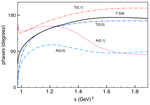
Figure 7: $S$-wave sector - top left: the continuous black curve (SW) is the modulus of the decay amplitude $T^{S}$, eq.(34), in arbitrary units, whereas other curves are moduli of partial contributions; top right: moduli of the $K\bar{K}$ scatterig amplitudes $A^{(0,1)}$, red curve, and $A^{(0,0)}$, blue curve; bottom: the continuous black curve (SW) is the phase of the decay amplitude $T^{S}$, eq.(34), and other continuous curves are phases of partial contributions; the dashed curves represent the phases of the $K\bar{K}$ scatterig amplitudes $A^{(0,1)}$ (red) and $A^{(0,0)}$ (blue).

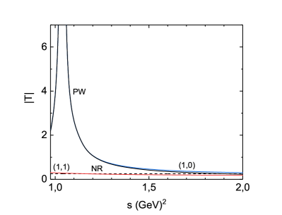
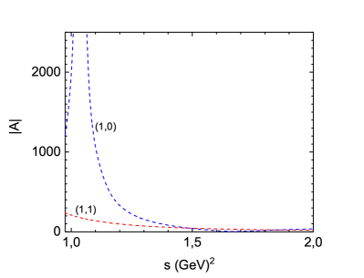
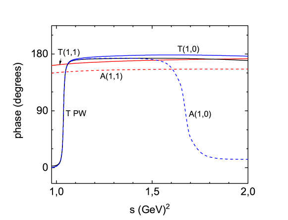
Figure 8: $P$-wave sector - top left: the continuous black curve (SW) is the modulus of the decay amplitude $T^{P}$, eq.(35), in arbitrary units, whereas other curves are moduli of partial contributions; top right: muduli of the $K\bar{K}$ scatterig amplitudes $A^{(1,1)}$, red curve, and $A^{(1,0)}$, blue curve; bottom: the continuous black curve (SW) is the phase of the decay amplitude $T^{S}$, eq.(34), and other continuous curves are phases of partial contributions; the dashed curves represent the phases of the $K\bar{K}$ scatterig amplitudes $A^{(1,1)}$ (red) and $A^{(1,0)}$ (blue).

In the sequence, we discuss some aspects of this relationship, using the low-energy parameters of Ref.EGPR , as if they could explain decay data. In Figs.7 and 8, we show the moduli and phases of the $S$- and $P$-wave decay amplitudes $T^{S}$, eq.(34) and $T^{P}$, eq.(35), together with the moduli and phases of the corresponding $K\bar{K}$ scattering amplitudes $A^{(J,I)}$. These figures illustrate the usefulness of the lagrangian approach. Without it, one would be able to determine just the full decay amplitudes $T^{S}$ and $T^{P}$, represented by the continuous black curves in the figures, and would not have access to partial contributions in different isospin channels. Moreover, it is also clear that one cannot guess the form of the $K\bar{K}$ scattering amplitudes $A^{(J,I)}$, represented by the red and blue dotted lines, from the decay components $T^{S}$ and $T^{P}$.

In Fig.9 we present the phase shifts and inelasticity parameters associated with the scattering amplitudes $A^{(J,I)}$. It important to stress that these figures correspond just to an exercise, since they are based on low-energy parameters. Nevertheless, they are instructive in showing the importance of the coupled channel structure, which is responsible for the inelasticities displayed. In the case of the I=1 $P$-wave, this related with the $\phi\rightarrow\pi\pi\pi$ channel, as discussed in App.C. In all cases, the bound $\eta\leq 1$ is satisfied.

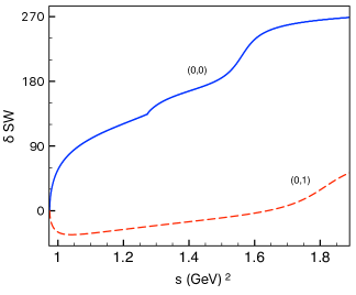
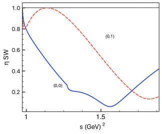
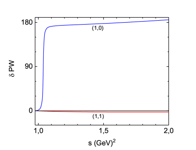
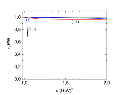
Figure 9: Phase shifts $\delta$ and inelasticity parameter $\eta$ for $K\bar{K}$ scattering - top: $S$-waves; bottom: $P$-waves; blue and red curves correspond respectively to isospin I=0 and I=1.

The Multi-Meson-Model we consider here yields scattering amplitudes involving dynamical features such: i) a chiral contact interaction in the two-body kernel, indicated in Fig.6; ii) the use of two resonances in the $(J=0,I=0)$ channel, preserving unitarity; iii) inclusion of coupled channels. In App.J we discuss their piecemeal relevance, in the case of $A^{(0,0)}$.

VI Summary

We propose a multi-meson-model (Triple-M) to describe the $D^{+}\to K^{-}K^{+}K^{+}$ decay, as a tool to extract information about $K\bar{K}$ scattering amplitudes. We depart from the dominance of the annihilation weak topology, which allows one to describe the whole decay process within the $SU(3)$ chiral symmetry framework. The non-resonant component is a proper three-body interaction that goes beyond the (2+1) approximation and is given by chiral symmetry as a real polynomium. Primary vertices describing the direct production of mesons and of lowest SU(3) resonances, in $S$- and $P$-waves, with isospin $0$ and $1$, are dressed by FSIs involving coupled channels. The $K\bar{K}$ scattering amplitudes for each of the $(J,I)$ considered are derived from the ChPTR LagrangianEGPR , unitarized by ressummation techniques in the $K$-matrix approximation, in which particle propagators were kept on-shell, and include coupled-channels. They are the only source of imaginary terms in the decay amplitude and fix the relative phase between $S$- and $P$-waves in Triple-M. This represents an important improvement over the isobar model, where this phase is a fitting parameter.

The fitting parameters in the Triple-M are resonance masses and coupling constants, which have a rather transparent physical meaning. Although they entered the Triple-M through the ChPTR Lagrangian, their meanings change so as to accommodate non-perturbation effects of meson-meson interactions. To obtain realistic values for these parameters, they should be extracted from a Triple-M fit to data. As a lesser alternative, here we employ the low-energy parametersEGPR values as if they resulted from data.

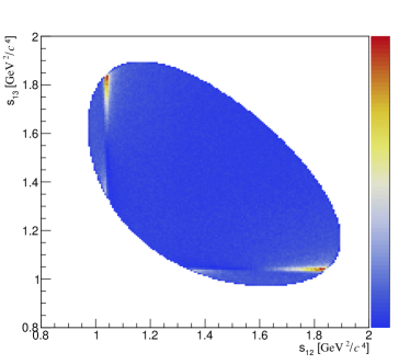
Figure 10: Toy Dalitz plot for Triple-M in $D^{+}\rightarrow K^{-}\,K^{+}\,K^{+}$ decay with arbitrary normalization.

In Fig.10, we show a toy Monte-Carlo Dalitz plot based on the Triple-M, where it is possible to see a destructive interference between the $S$- and $P$-waves on the low-energy sector of the $\phi(1020)$. One of the $\phi(1020)$ lobes is depleted with respect to the other, resulting in a peak and a dip, a behaviour similar to that observed in LHCb preliminary dataLHCbkkk .

In our one-dimensional toy studies, Figs.7-8, we show that the Triple-M can track the hidden isospin signatures of two-body interactions in three-body data, allowing one to disentangle the relative contributions of resonances $a_{0}(980)$ and $f_{0}(980)$. By comparing results for the three-body amplitudes $T^{J}$ and the scattering amplitudes $A^{(J,I)}$, it becomes clear that even though the later are present in the former, they cannot be extracted directly. However, with a model departing from a Lagrangian that includes a full two-body coupled channel dynamics, such as our Triple-M, fits to decay data can give rise to predictions for the $K\bar{K}$ scattering amplitudes $A^{(J,I)}$.

Appendix A kinematics

Momenta are defined by $D(P)\rightarrow K^{-}(p_{1})\,K^{+}(p_{2})\,K^{+}(p_{3})$, with $P=p_{1}+p_{2}+p_{3}$. The invariant masses read

$$m_{12}^{2}=(p_{1}\!+\!p_{2})^{2}=(P\!-\!p_{3})^{2}\;,$$ (36)

$$m_{13}^{2}=(p_{1}\!+\!p_{3})^{2}=(P\!-\!p_{2})^{2}\;,$$ (37)

$$m_{23}^{2}=(p_{2}\!+\!p_{3})^{2}=(P\!-\!p_{1})^{2}\;,$$ (38)

and satisfy the constraint

$$M^{2}=m_{12}^{2}+m_{13}^{2}+m_{23}^{2}-m_{1}^{2}-m_{2}^{2}-m_{3}^{2}\;.$$ (39)

Their values are also limited by the boundaries of the Dalitz plot, by

$$(m_{1}\!+\!m_{2})^{2}\leq m_{12}^{2}\leq(M-m_{3})^{2}\;,$$ (40)

$$(m_{1}\!+\!m_{3})^{2}\leq m_{13}^{2}\leq(M-m_{2})^{2}\;,$$ (41)

$$(m_{2}\!+\!m_{3})^{2}\leq m_{23}^{2}\leq(M-m_{1})^{2}\;.$$ (42)

Appendix B two-meson propagators and functions $\Omega$

Expressions presented here are conventional. They are displayed for the sake of completeness and rely on the the results of Ref.GL85 . These integrals do not include symmetry factors, which are accounted for in the main text. One deals with both $S$ and $P$ waves and the corresponding two-meson propagators are associated with the integrals

$$\left\{I_{ab};\,I_{ab}^{\mu\nu}\right\}=\int\frac{d^{4}\ell}{(2\pi)^{4}}\frac{\left\{1;\,\ell^{\mu}\ell^{\nu}\right\}}{D_{a}D_{b}},$$ (43)

$$D_{a}=(\ell\!+\!p/2)^{2}\!-\!M_{a}^{2}\;,\hskip 17.07164ptD_{b}=(\ell\!-\!p/2)^{2}\!-\!M_{b}^{2}\;,$$ (44)

with $p^{2}=s$. Both integrals $I_{ab}$ and $I_{ab}^{\mu\nu}$ are evaluated using dimensional techniquesGL85 . For $s\geq(M_{a}\!+\!M_{b})^{2}$, the function $I_{ab}$ has the structure

$$I_{ab} \!=\! i\;\frac{1}{16\pi^{2}}\,\left[\Lambda_{ab}+\Pi_{ab}\right]$$ (45)

where $\Lambda_{ab}$ is a divergent function of the renormalization scale $\mu$ and of the number of dimensions $n\,$, which diverges in the limit $n\rightarrow 4\,$, whereas $\Pi$ is regular component, given by

$$\Pi_{ab}(s)=1+\frac{m_{a}^{2}\!+\!m_{b}^{2}}{m_{a}^{2}-m_{b}^{2}}\,\ln\frac{m_{a}}{m_{b}}-\,\frac{m_{a}^{2}\!-\!m_{b}^{2}}{s}\,\ln\frac{m_{a}}{m_{b}}$$

$$-\,\frac{\sqrt{\lambda}}{s}\;\ln\left[\frac{s-m_{a}^{2}-m_{b}^{2}+\sqrt{\lambda}}{2\,m_{a}\,m_{b}}\right]+\,i\,\pi\;\frac{\sqrt{\lambda}}{s}\;,$$ (46)

$$\lambda=s^{2}-2\;s\;(m_{a}^{2}+m_{b}^{2})+(m_{a}^{2}-m_{b}^{2})^{2}\;.$$ (47)

which, for $a=b\,$, reduces to

$$\Pi_{aa}(s)=2-\,\frac{\sqrt{\lambda}}{s}\;\ln\left[\frac{s-2\,m_{a}^{2}+\sqrt{\lambda}}{2\,m_{a}^{2}}\right]+\,i\,\pi\;\frac{\sqrt{\lambda}}{s}\;.$$ (48)

The tensor integral is needed for $a=b\,$ only, and one has

$$I_{aa}^{\mu\nu} \!=\! i\;\frac{1}{16\pi^{2}}\,\left\{\frac{p^{\mu}\,p^{\nu}}{s}\,\left[\Lambda_{aa}^{pp}+\frac{1}{12}\left[s-4\,m_{x}^{2}\,\right]\;\Pi_{aa}\right]\right.$$ (49)

$$\!-\! \left.g^{\mu\nu}\,\left[\Lambda_{aa}^{g}+\frac{1}{12}\left[s-4\,m_{a}^{2}\,\right]\;\Pi_{aa}\right]\right\}\;,$$

where $\Lambda_{aa}^{pp}$ and $\Lambda_{aa}^{g}$ are divergent quantities.

In the $K$-matrix approximation, one keeps only the imaginary parts of the loop integrals, which are contained in the function $\Pi$ and has

$$\Pi_{ab} \!\rightarrow\! -\,\frac{1}{16\,\pi}\,\frac{\sqrt{\lambda}}{s}\;,$$ (50)

$$\Pi_{aa}^{\mu\nu} \!\rightarrow\! \frac{1}{192\,\pi}\,\left[g^{\mu\nu}-\frac{p^{\mu}p^{\nu}}{s}\right]\,\frac{\lambda^{3/2}}{s^{2}}\;.$$ (51)

In the decay calculation, it is more covenient to use the functions $\bar{\Omega}$, defined by

$$\Pi_{ab} \!\rightarrow\! -i\;\bar{\Omega}_{ab}^{S}\;,$$ (52)

$$\Pi_{aa}^{\mu\nu} \!\rightarrow\! \frac{i}{4}\,\left[g^{\mu\nu}-\frac{p^{\mu}p^{\nu}}{s}\right]\,\bar{\Omega}_{aa}^{P}\;.$$ (53)

These results are related with CM momenta by

$$\bar{\Omega}_{ab}^{S}=-\,\frac{i}{8\pi}\;\frac{Q_{ab}}{\sqrt{s}}\;\theta(s\!-\!(M_{a}\!+\!M_{b})^{2})\;,$$ (54)

$$\bar{\Omega}_{aa}^{P}=-\,\frac{i}{6\pi}\;\frac{Q_{aa}^{3}}{\sqrt{s}}\;\theta(s\!-\!4\,M_{a}^{2})\;,$$ (55)

$$Q_{ab}=\frac{1}{2}\,\sqrt{s-2\,(M_{a}^{2}+M_{b}^{2})+(M_{a}^{2}-M_{b}^{2})^{2}/s}\;,$$ (56)

where $\theta$ is the Heaviside step function.

Appendix C partially dressed $\phi$ propagator

The bare $\phi$ propagator, $G_{\alpha\beta\gamma\delta}$, is given by eq.(A.10) of Ref.EGPR . It is dressed by both $\pi\rho$ and $\bar{K}K$ intermediate states and the corresponding self-energies are denoted respectively by $\Sigma_{\pi\rho}$ and $\Sigma_{\bar{K}K}$. In this section we consider just contributions of the former kind. The full propagator is given by

$$i\,\Delta_{\alpha\beta\gamma\delta} \!=\! i\,\Delta_{\alpha\beta\gamma\delta}^{(0)}+i\,\Delta_{\alpha\beta\gamma\delta}^{(1)}+i\,\Delta_{\alpha\beta\gamma\delta}^{(2)}+i\,\Delta_{\alpha\beta\gamma\delta}^{(3)}+\cdots$$ (57)

$$i\,\Delta_{\alpha\beta\gamma\delta}^{(0)} \!=\! G_{\alpha\beta\gamma\delta}$$ (58)

$$i\,\Delta_{\alpha\beta\gamma\delta}^{(1)} \!=\! G_{\alpha\beta ab}\;\left[-i\,\Sigma^{abcd}\right]\;G_{cd\gamma\delta}$$ (59)

$$i\,\Delta_{\alpha\beta\gamma\delta}^{(2)} \!=\! G_{\alpha\beta ab}\;\left[-i\,\Sigma^{abef}\right]\;G_{efgh}\;\left[-i\,\Sigma^{ghcd}\right]\;G_{cd\gamma\delta}$$ (60)

The $\phi\pi\rho$ interaction is extracted from the lagrangian

$${\cal{L}}^{\omega_{1}} \!=\! i\,g_{1}\;\epsilon^{\mu\nu\rho\sigma}\;\partial^{\lambda}\omega_{1\,\lambda\mu}\;\left[\partial_{\nu}\pi^{-}\rho_{\rho\sigma}^{+}+\partial_{\nu}\pi^{+}\rho_{\rho\sigma}^{-}+\partial_{\nu}\pi^{0}\rho_{\rho\sigma}^{0}\right]$$ (61)

where $\omega_{1}=\cos\theta\,\phi-\sin\theta\,\omega$ is the singlet component. In the sequence, we write $g_{\epsilon}=g_{1}\,\cos\theta$.

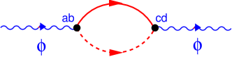
Figure 11: Intermediate $\pi\rho$ contribution to the $\phi$ self-energy.

The self energy is given by

$$-i\,\Sigma_{\rho\pi}^{abcd} \!=\! \frac{(k^{a}\,g^{b\mu}-g^{a\mu}\,k^{b})}{2}\;\left[H_{\mu\lambda}\right]\;\frac{(k^{c}\,g^{d\lambda}-g^{c\lambda}\,k^{d})}{2}\;,$$ (62)

$$H_{\mu\lambda} \!=\! \left[-3\,g_{\epsilon}^{2}\;I_{\mu\lambda}\right]\;,$$ (63)

$$I_{\mu\lambda} \!=\! \frac{1}{i}\;\int\!\!\frac{d^{4}\ell}{(2\pi)^{4}}\;\frac{p^{\mu}\,p^{\lambda}}{p^{2}-M_{\pi}^{2}}\;\epsilon_{\mu\nu\chi\eta}\,G_{\chi\eta\omega\zeta}(q)\,\epsilon_{\lambda\xi\omega\zeta}\;,$$ (64)

with $p=k/2-\ell,\;\;q=k/2+\ell$ and $k^{2}=s\,$. Using the explicit form of $G_{\chi\eta\omega\zeta}$ and the definitions $D_{\pi}=p^{2}-M_{\pi}^{2}\,,\;\;D_{\rho}=q^{2}-m_{\rho}^{2}$, we find

$$I_{\mu\lambda}\rightarrow\frac{4}{m_{\rho}^{2}}\;\int\!\!\frac{d^{4}\ell}{(2\pi)^{4}}\;\frac{1}{D_{\pi}}\;\frac{1}{D_{\rho}}\;$$ (65)

$$\times\left\{g_{\mu\lambda}\left[-m_{\rho}^{2}\left(M_{\pi}^{2}+D_{\pi}\right)+\frac{1}{4}\,\left(s-M_{\pi}^{2}-m_{\rho}^{2}-D_{\pi}-D_{\rho}\right)^{2}\right]+\ell_{\mu}\ell_{\lambda}\left[k^{2}-D_{\rho}\right]\right\}\;,$$

where we have used the fact that terms proportional to $k_{\mu}$ and $k_{\lambda}$ do not contribute to eq.(62). This integral is highly divergent, but the part regarding the $K\rho$ cut is not. Terms containing factors $D_{\pi}$ and $D_{\rho}$ in the numerator do not contribute to the cut function and the relevant integral is

$$I_{\mu\lambda}\!\rightarrow\frac{1}{m_{\rho}^{2}}\;\int\!\!\frac{d^{4}\ell}{(2\pi)^{4}}\;\frac{1}{D_{\pi}\;D_{\rho}}\left\{\left[s^{2}-2\,s\,\left(M_{\pi}^{2}+m_{\rho}^{2}\right)+\left(M_{\pi}^{2}-m_{\rho}^{2}\right)^{2}\right]g_{\mu\lambda}+4\,s\,\ell_{\mu}\ell_{\lambda}\right\}\;.$$ (66)

Using the definition

$$I_{\pi\rho}=\int\!\!\frac{d^{4}\ell}{(2\pi)^{4}}\;\frac{1}{D_{\pi}\;D_{\rho}}$$ (67)

and the result

$$\int\!\!\frac{d^{4}\ell}{(2\pi)^{4}}\;\frac{\ell_{\mu}\,\ell_{\lambda}}{D_{\pi}\;D_{\rho}}\; \!=\! -\left\{\frac{1}{12\,k^{2}}\;\left[s^{2}-2\,s\,(M_{\pi}^{2}+m_{\rho}^{2})+(M_{\pi}^{2}-m_{\rho}^{2})^{2}\right]\,I_{\pi\rho}\right\}g_{\mu\lambda}$$ (68)

$$\!+\! \mathrm{term}\,\mathrm{proportional}\,\mathrm{to}\,k_{\mu}\,k_{\lambda}\;,$$

the relevant component of $I_{\mu\lambda}$ becomes

$$I_{\mu\lambda} \!\rightarrow\! \left\{\frac{2}{3\,m_{\rho}^{2}}\;\left[s^{2}-2\,s\,(M_{\pi}^{2}+m_{\rho}^{2})+(M_{\pi}^{2}-m_{\rho}^{2})^{2}\right]\;I_{\pi\rho}\right\}\;g_{\mu\lambda}\;.$$ (69)

The on-shell contribution to eq.(67) is given by

$$I_{\pi\rho} \!=\! -\;\frac{1}{16\,\pi}\frac{\sqrt{\lambda_{\pi\rho}}}{s}\;,$$ (70)

with $\lambda_{\pi\rho}=\left[s^{2}-2\,s\,(M_{\pi}^{2}+m_{\rho}^{2})+(M_{\pi}^{2}-m_{\rho}^{2})^{2}\right]=4\,s\,Q_{\pi\rho}^{2}$, where $Q_{\pi\rho}$ is the CM three-momentum. We then have

$$H_{\mu\lambda}=g_{\mu\lambda}\,\frac{m_{\phi}}{s}\;\Gamma_{\phi}^{\pi\rho}(s)\;,$$ (71)

$$m_{\phi}\,\Gamma_{\phi}^{\pi\rho}(s)=\frac{g_{\epsilon}^{2}}{\pi\,m_{\rho}^{2}}\;s^{3/2}\;Q_{\pi\rho}^{3}\;.$$ (72)

Numerically, $\Gamma_{\phi}^{\pi\rho}=0.1532\times\Gamma_{\phi}=0.1532\times 0.004247\,$GeVPDG . Using this result into eq.(57) and ressumming the series, we get the partially dressed propagator

$$i\,\Delta_{\alpha\beta\gamma\delta}^{\pi\rho} \!=\! G_{\alpha\beta\gamma\delta}$$

$$\!+\! \left[\frac{i\,m_{\phi}\,\Gamma_{\phi}^{\pi\rho}(s)/s}{D_{\phi}^{\pi\rho}(s)}\right]\frac{1}{2}\left[g_{\alpha}^{d}\,k_{\beta}\,k^{c}+g_{\beta}^{c}\,k_{\alpha}\,k^{d}-g_{\alpha}^{c}\,k_{\beta}\,k^{d}-g_{\beta}^{d}\,k_{\alpha}\,k^{c}\right]\;G_{cd\gamma\delta}\;,$$

where the denominator $D_{\phi}^{\pi\rho}(s)$ is given by

$$D_{\phi}^{\pi\rho} \!=\! s-m_{\phi}^{2}+i\,m_{\phi}\,\Gamma_{\phi}^{\pi\rho}(s)\;.$$ (74)

In the evaluation of amplitudes involving a $\bar{K}(p_{1})\,K(p_{2})$ vertex, one encounters the product

$$i\,\Delta_{\alpha\beta\gamma\delta}\,\left(p_{1}^{\gamma}\,p_{2}^{\delta}-p_{2}^{\gamma}\,p_{1}^{\delta}\right) \!=\! -\,\frac{2\,i}{D_{\phi}^{\pi\rho}(s)}\;\left(p_{1\alpha}\,p_{2\beta}-p_{2\alpha}\,p_{1\beta}\right)\;.$$ (75)

Appendix D SU(3) intermediate states

In the treatment of intermediate states, it is convenient to work with Cartesian $SU(3)$ states, which are related to charged states by

$$|\pi^{+}\rangle=-|1+i\,2\rangle/\sqrt{2}\;,\hskip 28.45274pt|\pi^{-}\rangle=|1-i\,2\rangle/\sqrt{2}\;,$$ (76)

$$|\pi^{0}\rangle=|3\rangle\;,\hskip 85.35826pt|\eta_{8}\rangle=|8\rangle\;,$$ (77)

$$|K^{+}\rangle=|4+i\,5\rangle/\sqrt{2}\;,\hskip 28.45274pt|K^{-}\rangle=-|4-i\,5\rangle/\sqrt{2}\;,$$ (78)

$$|K^{0}\rangle=|6+i\,7\rangle/\sqrt{2}\;,\hskip 28.45274pt|\bar{K}^{0}\rangle=|6-i\,7\rangle/\sqrt{2}\;.$$ (79)

We need just two-meson intermediate states $|ab\rangle$, with the same quantum numbers as the $K^{-}K^{+}$ system, which are given by

$$|V_{3}^{\pi\pi}\rangle \!=\! (1/\sqrt{2})\,|1\,2-2\,1\rangle,$$ (80)

$$|V_{3}^{KK}\rangle \!=\! (1/2)\,|4\,5-5\,4-6\,7+7\,6\rangle,$$ (81)

$$|V_{8}^{KK}\rangle \!=\! (1/2)\,|4\,5-5\,4+6\,7-7\,6\rangle,$$ (82)

$$|U_{3}^{\pi 8}\rangle \!=\! (1/\sqrt{2})\,|3\,8+8\,3\rangle,$$ (83)

$$|U_{3}^{KK}\rangle \!=\! (1/2)\,|4\,4+5\,5-6\,6-7\,7\rangle,$$ (84)

$$|S^{\pi\pi}\rangle \!=\! (1/\sqrt{3})\,|1\,1+2\,2+3\,3\rangle,$$ (85)

$$|S^{KK}\rangle \!=\! (1/2)\,|4\,4+5\,5+6\,6+7\,7\rangle,$$ (86)

$$|S^{88}\rangle \!=\! |8\,8\rangle.$$ (87)

The state $|K^{-}K^{+}\rangle$ includes a conventional phase an reads

$$|K^{-}K^{+}\rangle \!=\! -(1/2)\,|(4-i\,5)(4+i\,5)\rangle=-(1/2)\,|4\,4+5\,5\rangle-i\,(1/2)\,|4\,5-5\,4\rangle$$ (88)

and, therefore,

$$\langle K^{-}\,K^{+}| \!=\! (i/2)\,\langle V_{3}^{KK}+V_{8}^{KK}|-(1/2)\,\langle U_{3}^{KK}+S^{KK}|.$$ (89)

Appendix E tree decay sub-amplitudes

In the evaluation of intermediate state contributions shown in diagrams of Fig.5, we need tree level contribution for the process $D\rightarrow a\,b\,K^{+}$, denoted by $T_{(0)}^{(J,I)}$, for spin $J$ and isospin $I$. In the results displayed below, the first terms correspond to resonances in diagrams (3A+3B), whereas those within square brackets, labeled by $c$, represent contact interactions in the top vertices of diagrams 2A and 2B. Using the constant $C$ defined in eq.(22), we have

$$[J,I=1,1]\rightarrow\langle V_{3}^{ab}\,K^{+}|\,T_{(0)}^{(1,1)}\,|\,D\rangle=\frac{i}{2}\,(m_{13}^{2}-m_{23}^{2})\;\Gamma_{(0)\,a\,b}^{(1,1)}\,,$$ (90)

$$\Gamma_{(0)\,\pi\pi}^{(1,1)}=C\left\{\left[\frac{\sqrt{2}\,G_{V}^{2}}{F^{2}}\right]\,\frac{m_{12}^{2}}{m_{12}^{2}-m_{\rho}^{2}}+\left[-\,\frac{1}{\sqrt{2}}\right]_{c}\right\},$$ (91)

$$\Gamma_{(0)\,KK}^{(1,1)}=C\left\{\left[\frac{G_{V}^{2}}{F^{2}}\right]\,\frac{m_{12}^{2}}{m_{12}^{2}-m_{\rho}^{2}}+\left[-\,\frac{1}{2}\right]_{c}\right\}$$ (92)

$$[J,I=1,0]\rightarrow\langle V_{8}^{KK}\,K^{+}|\,T_{(0)}^{(1,0)}\,|\,D\rangle=\frac{i}{2}\,(m_{13}^{2}-m_{23}^{2})\;\Gamma_{(0)\,KK}^{(1,0)}\,,$$ (93)

$$\Gamma_{(0)\,KK}^{(1,0)}=C\left\{\left[\frac{3\,G_{V}^{2}}{F^{2}}\,\sin^{2}\!\theta\right]\,\frac{m_{12}^{2}}{D_{\phi}^{\pi\rho}(m_{12}^{2})}+\left[-\,\frac{3}{2}\right]_{c}\right\},$$ (94)

Here, the function $D_{\phi}^{\pi\rho}$ is a partially dressed $\phi$ propagator, discussed in App.C, eq.(74), associated with the partial width of the decay $\phi\rightarrow(\rho\pi+\pi\pi\pi)$.

$$[J,I=0,1]\rightarrow\langle U_{3}^{ab}\,K^{+}|\,T_{(0)}^{(0,1)}\,|\,D\rangle=\Gamma_{(0)\,a\,b}^{(0,1)}\,,$$ (95)

$$\Gamma_{(0)\,\pi 8}^{(0,1)}=C\left\{\left[\frac{2\,\sqrt{2}}{\sqrt{3}\,F^{2}}\right]\;\frac{\left[-c_{d}\,P\!\cdot\!p_{3}+c_{m}\,M_{D}^{2}\right]}{m_{12}^{2}-m_{a_{0}}^{2}}\left[c_{d}\,\left(m_{12}^{2}-M_{\pi}^{2}-M_{8}^{2}\right)+2\,c_{m}\,M_{\pi}^{2}\right]\right.$$

$$\left.+\left[-\,\frac{\sqrt{3}}{\sqrt{2}}\,\left[\,M_{D}^{2}/3-P\!\cdot\!p_{3}\right]\right]_{c}\right\},$$ (96)

$$\Gamma_{(0)\,KK}^{(0,1)}=C\left\{\left[\frac{2}{F^{2}}\right]\;\frac{\left[-c_{d}\,P\!\cdot\!p_{3}+c_{m}\,M_{D}^{2}\right]}{m_{12}^{2}-m_{a_{0}}^{2}}\left[c_{d}\,\left(m_{12}^{2}-2M_{K}^{2}\right)+2\,c_{m}\,M_{K}^{2}\right]\right.$$

$$\left.+\left[-\,\frac{1}{2}\left[M_{D}^{2}-P\!\cdot\!p_{3}\right]\right]_{c}\right\},$$ (97)

$$[J,I=0,0]\rightarrow\langle S^{ab}\,K^{+}|\,T_{(0)}^{(0,0)}\,|\,D\rangle=\Gamma_{(0)\,a\,b}^{(0,0)}\,,$$ (98)

$$\Gamma_{(0)\,\pi\pi}^{(0,0)}=C\left\{\left[\frac{8\sqrt{3}}{F^{2}}\right]\;\frac{\left[-\tilde{c}_{d}\,P\!\cdot\!p_{3}+\tilde{c}_{m}\,M_{D}^{2}\right]}{m_{12}^{2}-m_{S1}^{2}}\;\left[\tilde{c}_{d}\,\left(m_{12}^{2}-2M_{\pi}^{2}\right)+2\,\tilde{c}_{m}\,M_{\pi}^{2}\right]\right.$$

$$\left.-\;\left[\frac{2}{\sqrt{3}\,F^{2}}\right]\;\frac{\left[-c_{d}\,P\!\cdot\!p_{3}+c_{m}\,M_{D}^{2}\right]}{m_{12}^{2}-m_{So}^{2}}\;\left[c_{d}\,\left(m_{12}^{2}-2M_{\pi}^{2}\right)+2\,c_{m}\,M_{\pi}^{2}\right]\right.$$

$$\left.+\left[-\,\frac{\sqrt{3}}{2}\,\left[M_{D}^{2}-P\!\cdot\!p_{3}\right]\right]_{c}\right\},$$ (99)

$$\Gamma_{(0)\,KK}^{(0,0)}=C\left\{\left[\frac{16}{F^{2}}\right]\;\frac{\left[-\tilde{c}_{d}\,P\!\cdot\!p_{3}+\tilde{c}_{m}\,M_{D}^{2}\right]}{m_{12}^{2}-m_{S1}^{2}}\;\left[\tilde{c}_{d}\,\left(m_{12}^{2}-2M_{K}^{2}\right)+2\,\tilde{c}_{m}\,M_{K}^{2}\right]\right.$$

$$\left.+\;\left[\frac{2}{3\,F^{2}}\right]\;\frac{\left[-c_{d}\,P\!\cdot\!p_{3}+c_{m}\,M_{D}^{2}\right]}{m_{12}^{2}-m_{So}^{2}}\left[c_{d}\,\left(m_{12}^{2}-2M_{K}^{2}\right)+2\,c_{m}\,M_{K}^{2}\right]\right.$$

$$\left.+\left[-\,\frac{3}{2}\,\left[M_{D}^{2}-P\!\cdot\!p_{3}\right]\right]_{c}\right\},$$ (100)

$$\Gamma_{(0)\,88}^{(0,0)}=C\left\{\left[\frac{8}{F^{2}}\right]\;\frac{\left[-\tilde{c}_{d}\,P\!\cdot\!p_{3}+\tilde{c}_{m}\,M_{D}^{2}\right]}{m_{12}^{2}-m_{S1}^{2}}\;\left[\tilde{c}_{d}\,\left(m_{12}^{2}-2M_{8}^{2}\right)+2\,\tilde{c}_{m}\,M_{8}^{2}\right]\right.$$

$$\left.+\;\left[\frac{2}{3\,F^{2}}\right]\;\frac{\left[-c_{d}\,P\!\cdot\!p_{3}+c_{m}\,M_{D}^{2}\right]}{m_{12}^{2}-m_{So}^{2}}\left[c_{d}\,\left(m_{12}^{2}-2M_{8}^{2}\right)+c_{m}\,\left(-10M_{\pi}^{2}+16M_{K}^{2}\right)/3\right]\right.$$

$$\left.+\left[-\,\frac{1}{2}\,\left[5\,M_{D}^{2}/3-3\,P\!\cdot\!p_{3}\right]\right]_{c}\right\}.$$ (101)

with

$$P\!\cdot\!p_{3}=\frac{1}{2}\left[M_{D}^{2}+M_{K}^{2}-m_{12}^{2}\right]\,.$$ (102)

Appendix F scattering kernels

The intermediate scattering amplitudes depend on interaction kernels in the four channels considered, associated with $J,I=1,0$. The kernel matrix elements for the reaction $c\,d\rightarrow a\,b$ are written as $\langle cd\,|\,{\cal{K}}^{J,I}\,|\,ab\rangle$, in terms of the states defined in App.D, and displayed below. All kernels are written as sums of NLO resonance contributions and chiral polynomials, involving both LO and NLO terms. The NLO polynomials are derived by assuming that the LECs are saturared by intermedate vector and scalar resonances, with masses $M_{V}$ and $M_{S}$, respectively. The kernel matrix elements read

$$[J,I=1,1]\rightarrow\langle V_{3}^{ab}\,|\,{\cal{K}}^{(1,1)}\,|\,V_{3}^{cd}\rangle=(t\!-\!u)\;{\cal{K}}_{(ab|cd)}^{(1,1)}$$ (103)

$${\cal{K}}_{(\pi\pi|\pi\pi)}^{(1,1)}=-2\,\left[\frac{G_{V}^{2}}{F^{4}}\right]\;\frac{s}{s-m_{\rho}^{2}}+\left[\frac{1}{F^{2}}\right]_{c}$$ (104)

$${\cal{K}}_{(\pi\pi|KK)}^{(1,1)}=-\sqrt{2}\,\left[\frac{G_{V}^{2}}{F^{4}}\right]\;\frac{s}{s-m_{\rho}^{2}}+\left[\frac{\sqrt{2}}{2\,F^{2}}\right]_{c}$$ (105)

$${\cal{K}}_{(KK|KK)}^{(1,1)}=-\left[\frac{G_{V}^{2}}{F^{4}}\right]\;\frac{s}{s-m_{\rho}^{2}}+\left[\frac{1}{2\,F^{2}}\right]_{c}$$ (106)

$$[J,I=1,0]\rightarrow\langle V_{8}^{ab}\,|\,{\cal{K}}^{(1,0)}\,|\,V_{8}^{cd}\rangle=(t\!-\!u)\;{\cal{K}}_{(ab|cd)}^{(1,0)}$$ (107)

$${\cal{K}}_{(KK|KK)}^{(1,0)}=-3\,\left[\frac{G_{V}^{2}\;\sin^{2}\!\theta}{F^{4}}\right]\;\frac{s}{D_{\phi}^{\pi\rho}}+\left[\frac{3}{2\,F^{2}}\right]_{c}$$ (108)

The function $D_{\phi}^{\pi\rho}$ is this expression represents a partially dressed $\phi$ propagator, discussed in App.C, eq.(74), and accounts for the partial width of the decay $\phi\rightarrow(\rho\pi+\pi\pi\pi)$.

$$[J,I=0,1]\rightarrow\langle U_{3}^{ab}\,|\,{\cal{K}}^{(0,1)}\,|\,U_{3}^{cd}\rangle={\cal{K}}_{(ab|cd)}^{(0,1)}$$ (109)

$${\cal{K}}_{(\pi 8|\pi 8)}^{(0,1)}=-\,\frac{1}{s-m_{a_{0}}^{2}}\,\left[\frac{4}{3\,F^{4}}\right]\;\left[c_{d}\,(s\!-\!M_{\pi}^{2}\!-\!M_{8}^{2})+c_{m}\,2M_{\pi}^{2}\right]^{2}+\left[\frac{2M_{\pi}^{2}}{3F^{2}}\right]_{c}$$ (110)

$${\cal{K}}_{(\pi 8|KK)}^{(0,1)}=-\,\frac{1}{s-m_{a_{0}}^{2}}\,\left[\frac{2\sqrt{2}}{\sqrt{3}\,F^{4}}\right]\left[c_{d}\,(s\!-\!M_{\pi}^{2}\!-\!M_{8}^{2})+c_{m}\,2M_{\pi}^{2}\right]\,\left[c_{d}\,s-(c_{d}\!-\!c_{m})\,2M_{K}^{2}\right]$$

$$+\left[\frac{(3s-4M_{K}^{2})}{\sqrt{6}\,F^{2}}\right]_{c}$$ (111)

$${\cal{K}}_{(KK|KK)}^{(0,1)}=-\frac{1}{s-m_{a_{0}}^{2}}\,\left[\frac{2}{F^{4}}\right]\;\left[c_{d}\,s-(c_{d}\!-\!c_{m})\,2M_{K}^{2}\right]^{2}+\left[\frac{s}{2F^{2}}\right]_{c}$$ (112)

$$[J,I=0,0]\rightarrow\langle S^{ab}\,|\,{\cal{K}}^{(0,0)}\,|\,S^{cd}\rangle={\cal{K}}_{(ab|cd)}^{(0,0)}$$ (113)

$${\cal{K}}_{(\pi\pi|\pi\pi)}^{(0,0)}=-\,\frac{1}{s-m_{S1}^{2}}\,\left[\frac{12}{F^{4}}\right]\;\left[\tilde{c}_{d}\,s-(\tilde{c}_{d}\!-\!\tilde{c}_{m})\,2M_{\pi}^{2}\right]^{2}$$

$$-\,\frac{1}{s-m_{So}^{2}}\,\left[\frac{2}{F^{4}}\right]\;\left[c_{d}\,s-(c_{d}\!-\!c_{m})\,2M_{\pi}^{2}\right]^{2}+\left[\frac{2s-M_{\pi}^{2}}{F^{2}}\right]_{c}$$ (114)

$${\cal{K}}_{(\pi\pi|KK)}^{(0,0)}=-\,\frac{1}{s-m_{S1}^{2}}\,\left[\frac{8\sqrt{3}}{F^{4}}\right]\;\left[\tilde{c}_{d}\,s-(\tilde{c}_{d}\!-\!\tilde{c}_{m})\,2M_{\pi}^{2}\right]\,\left[\tilde{c}_{d}\,s-(\tilde{c}_{d}\!-\!\tilde{c}_{m})\,2M_{K}^{2}\right]$$

$$+\frac{1}{s-m_{So}^{2}}\,\left[\frac{2}{\sqrt{3}\,F^{4}}\right]\;\left[c_{d}\,s-(c_{d}\!-\!c_{m})\,2M_{\pi}^{2}\right]\left[c_{d}\,s-(c_{d}\!-\!c_{m})\,2M_{K}^{2}\right]+\left[\frac{\sqrt{3}\,s}{2F^{2}}\right]_{c}$$ (115)

$${\cal{K}}_{(\pi\pi|88)}^{(0,0)}=-\,\frac{1}{s-m_{S1}^{2}}\,\left[\frac{4\sqrt{3}}{F^{4}}\right]\;\left[\tilde{c}_{d}\,s-(\tilde{c}_{d}\!-\!\tilde{c}_{m})\,2M_{\pi}^{2}\right]\,\left[\tilde{c}_{d}\,s-(\tilde{c}_{d}\!-\!\tilde{c}_{m})\,2M_{8}^{2}\right]$$

$$+\frac{1}{s-m_{So}^{2}}\,\left[\frac{2}{\sqrt{3}\,F^{4}}\right]\;\left[c_{d}\,s-(c_{d}\!-\!c_{m})\,2M_{\pi}^{2}\right]\left[c_{d}\,(s\!-\!2M_{8}^{2})+c_{m}\,(16M_{K}^{2}\!-\!10M_{\pi}^{2})/3\right]$$

$$+\,\left[\frac{\sqrt{3}\,M_{\pi}^{2}}{3F^{2}}\right]_{c}$$ (116)

$${\cal{K}}_{(KK|KK)}^{(0,0)}=-\,\frac{1}{s-m_{S1}^{2}}\,\left[\frac{16}{F^{4}}\right]\;\left[\tilde{c}_{d}\,s-(\tilde{c}_{d}\!-\!\tilde{c}_{m})\,2M_{K}^{2}\right]^{2}$$

$$-\frac{1}{s-m_{So}^{2}}\,\left[\frac{2}{3\,F^{4}}\right]\;\left[c_{d}\,s-(c_{d}\!-\!c_{m})\,2M_{K}^{2}\right]^{2}+\left[\frac{3s}{2F^{2}}\right]_{c}$$ (117)

$${\cal{K}}_{(KK|88)}^{(0,0)}=-\,\frac{1}{s-m_{S1}^{2}}\,\left[\frac{8}{F^{4}}\right]\;\left[\tilde{c}_{d}\,s-(\tilde{c}_{d}\!-\!\tilde{c}_{m})\,2M_{K}^{2}\right]\,\left[\tilde{c}_{d}\,s-(\tilde{c}_{d}\!-\!\tilde{c}_{m})\,2M_{8}^{2}\right]$$

$$-\,\frac{1}{s-m_{So}^{2}}\,\left[\frac{2}{3\,F^{4}}\right]\;\left[c_{d}\,s-(c_{d}\!-\!c_{m})\,2M_{K}^{2}\right]\left[c_{d}\,(s\!-\!2M_{8}^{2})+c_{m}\,(16M_{K}^{2}\!-\!10M_{\pi}^{2})/3\right]$$

$$+\,\left[\frac{9s-8M_{K}^{2}}{6F^{2}}\right]_{c}$$ (118)

$${\cal{K}}_{(88|88)}^{(0,0)}=-\,\frac{1}{s-m_{S1}^{2}}\,\left[\frac{4}{F^{4}}\right]\;\left[\tilde{c}_{d}\,s-(\tilde{c}_{d}\!-\!\tilde{c}_{m})\,2M_{8}^{2}\right]^{2}$$

$$-\,\frac{1}{s-m_{So}^{2}}\,\left[\frac{2}{3\,F^{4}}\right]\;\left[c_{d}\,(s\!-\!2M_{8}^{2})+c_{m}\,(16M_{K}^{2}\!-\!10M_{\pi}^{2})/3\right]^{2}$$

$$+\,\left[\frac{-7M_{\pi}^{2}+16M_{K}^{2}}{9F^{2}}\right]_{c}$$ (119)

Appendix G channel dependent decay amplitudes - full results

The tree level decay amplitudes for channel with spin $J$ and isospin $I$, given in App.E, are written as

$$\langle X^{ab}\,K^{+}|\,T_{(0)}^{(J,I)}\,|\,D\rangle \!=\! \frac{i}{2}\,(m_{13}^{2}-m_{23}^{2})\;\Gamma_{(0)\,a\,b}^{(1,I)}\;\;\;\rightarrow(X=V_{3},V_{8})$$ (120)

$$\!=\! \Gamma_{(0)\,a\,b}^{(0,I)}\;\;\;\rightarrow(X=U_{3},S)$$

The full amplitudes are obtained by including all possible final state interactions, as indicated in Figs.5 and 6. The terms involving a single meson-meson interaction read

$$\langle X^{ab}\,K^{+}|\,T_{(1)}^{(J,I)}\,|\,D\rangle \!=\! \frac{i}{2}\,(m_{13}^{2}-m_{23}^{2})\;\Gamma_{(1)\,a\,b}^{(1,I)}\;\;\;\rightarrow(X=V_{3},V_{8})$$ (121)

$$\!=\! \Gamma_{(1)\,a\,b}^{(0,I)}\;\;\;\rightarrow(X=U_{3},S)$$

with

$$\Gamma_{(1)\,ab}^{(J,I)}=\sum_{cd}\;\,M_{ab|cd}^{(J,I)}\;\Gamma_{(0)\,cd}^{(J,I)}\,,$$ (122)

$$M_{ab|cd}^{(J,I)}=-{\cal{K}}_{ab|cd}^{(J,I)}\,\left[S_{F}\,\bar{\Omega}_{cd}^{J}\right]\;.$$ (123)

where ${\cal{K}}_{ab|cd}^{(J,I)}$ are the scattering kernels displayed in App.F, $\bar{\Omega}_{cd}^{J}$ are the two-meson propagators given in App.B, and the symmetry factor $S_{F}=1\rightarrow c\neq d$ and $S_{F}=1/2\rightarrow c=d$. The terms $\Gamma_{(2)\,a\,b}^{(J,I)}$, containing two meson-meson interactions are constructed in a similar way from $\Gamma_{(1)\,a\,b}^{(J,I)}$, and so on.

The inclusion of all possible meson-meson interactions leads to the infinite geometric series

$$\Gamma_{ab}^{(J,I)}=\sigma_{ab|cd}^{(J,I)}\;\Gamma_{(0)\,cd}^{(J,I)}\;,$$ (124)

$$\sigma_{ab|cd}^{(J,I)}=\left\{1+M^{(J,I)}+[M^{(J,I)}]^{2}+\cdots\right\}_{ab|cd}\;,$$ (125)

where $\sigma^{(J,I)}$ is its sum, given by

$$\sigma^{(J,I)}=\left[1-M^{(J,I)}\right]^{-1}\;.$$ (126)

Thus, decay amplitude reads formally

$$\Gamma^{(J,I)}=\left[1-M^{(J,I)}\right]^{-1}\,\Gamma_{(0)}^{(J,I)}\;.$$ (127)

and encompasses a coupled channel structure, which depends on the spin-isospin considered.

In order to display the meaning of the indices used in this structure, we label informally each $(J,I)$ channel by its most prominent resonance and recall that
$\rho$-channel: $\Gamma_{(0)\,11}^{(1,1)}\!\!=\!\!\Gamma_{(0)\,\pi\pi}^{(1,1)}\,,\Gamma_{(0)\,22}^{(1,1)}\!\!=\!\!\Gamma_{(0)\,KK}^{(1,1)}\,$;
$\phi$-channel: $\Gamma_{(0)}^{(1,0)}\!\!=\!\!\Gamma_{(0)\,KK}^{(1,0)}\,$;
$a_{0}$-cannel: $\Gamma_{(0)\,11}^{(0,1)}\!\!=\!\!\Gamma_{(0)\,\pi 8}^{(0,1)}\,,\Gamma_{(0)\,22}^{(0,1)}\!\!=\!\!\Gamma_{(0)\,KK}^{(0,1)}\,$;
$f_{0}$-channel: $\Gamma_{(0)\,11}^{(0,0)}\!\!=\!\!\Gamma_{(0)\,\pi\pi}^{(0,0)}\,,\Gamma_{(0)\,22}^{(0,0)}\!\!=\!\!\Gamma_{(0)\,KK}^{(0,0)}\,,\Gamma_{(0)\,33}^{(0,0)}\!\!=\!\!\Gamma_{(0)\,88}^{(0,0)}\,$.
The meanings of the indices used in the matrices $M^{(J,I)}$, eq.(123), are similar.

In this work, we need at most three coupled channels, which corresponds to

$$\sigma=\frac{1}{\det[1-M]}$$

$$\times\left[\matrix{[1\!-\!M_{22}][1\!-\!M_{33}]\!-\!M_{23}M_{32}&M_{12}[1\!-\!M_{33}]\!+\!M_{13}M_{32}&M_{13}[1\!-\!M_{22}]\!+\!M_{12}M_{23}\cr M_{21}[1\!-\!M_{33}]\!+\!M_{23}M_{31}&[1\!-\!M_{11}][1\!-\!M_{33}]\!-\!M_{13}M_{31}&M_{23}[1\!-\!M_{11}]\!+\!M_{13}M_{21}\cr M_{31}[1\!-\!M_{22}]\!+\!M_{21}M_{32}&M_{32}[1\!-\!M_{11}]\!+\!M_{12}M_{31}&[1\!-\!M_{11}][1\!-\!M_{22}]\!-\!M_{12}M_{21}}\right]$$

$$\det(1-M)=[1\!-\!M_{11}][1\!-\!M_{22}][1\!-\!M_{33}]-[1\!-\!M_{11}]M_{23}M_{32}-[1\!-\!M_{22}]M_{13}M_{31}$$

$$-[1\!-\!M_{33}]M_{12}M_{21}-M_{12}M_{23}M_{31}-M_{21}M_{32}M_{13}$$ (128)

In the $K$-matrix approximation, the matrix elements $M$ are purely imaginary, owing to the presence of the two-meson propagator. The explicit functions to be used in the calculation are displayed below.

$$M_{11}^{(1,1)}=-{\cal{K}}_{\pi\pi|\pi\pi}^{(1,1)}\,[\bar{\Omega}_{\pi\pi}^{P}/2]\;,\hskip 28.45274ptM_{12}^{(1,1)}=-{\cal{K}}_{\pi\pi|KK}^{(1,1)}\,[\bar{\Omega}_{KK}^{P}/2]\;,$$

$$M_{21}^{(1,1)}=-{\cal{K}}_{\pi\pi|KK}^{(1,1)}\,[\bar{\Omega}_{\pi\pi}^{P}/2]\;,\hskip 28.45274ptM_{22}^{(1,1)}=-{\cal{K}}_{KK|KK}^{(1,1)}\,[\bar{\Omega}_{KK}^{P}/2]\;.$$ (129)

$$M^{(1,0)}=-{\cal{K}}_{KK|KK}^{(1,0)}\,[\bar{\Omega}_{KK}^{P}/2]\;.$$ (130)

$$M_{11}^{(0,1)}=-{\cal{K}}_{\pi 8|\pi 8}^{(0,1)}\,[\bar{\Omega}_{\pi 8}^{S}/2]\;,\hskip 28.45274ptM_{12}^{(0,1)}=-{\cal{K}}_{\pi 8|KK}^{(0,1)}\,[\bar{\Omega}_{KK}^{S}/2]\;,$$

$$M_{21}^{(0,1)}=-{\cal{K}}_{\pi 8|KK}^{(0,1)}\,[\bar{\Omega}_{\pi 8}^{S}/2]\;,\hskip 28.45274ptM_{22}^{(0,1)}=-{\cal{K}}_{KK|KK}^{(0,1)}\,[\bar{\Omega}_{KK}^{S}/2]\;.$$ (131)

$$M_{11}^{(0,0)}=-{\cal{K}}_{\pi\pi|\pi\pi}^{(0,0)}\,[\bar{\Omega}_{\pi\pi}^{S}/2]\;,\hskip 28.45274ptM_{12}^{(0,0)}=-{\cal{K}}_{\pi\pi|KK}^{(0,0)}\,[\bar{\Omega}_{KK}^{S}/2]\;,$$

$$M_{13}^{(0,0)}=-{\cal{K}}_{\pi\pi|88}^{(0,0)}\,[\bar{\Omega}_{88}^{S}/2]\;,\hskip 28.45274ptM_{21}^{(0,0)}=-{\cal{K}}_{\pi\pi|KK}^{(0,0)}\,[\bar{\Omega}_{\pi\pi}^{S}/2]\;,$$

$$M_{22}^{(0,0)}=-{\cal{K}}_{KK|KK}^{(0,0)}\,[\bar{\Omega}_{KK}^{S}/2]\;,\hskip 28.45274ptM_{23}^{(0,0)}=-{\cal{K}}_{KK|88}^{(0,0)}\,[\bar{\Omega}_{88}^{S}/2]\;,$$

$$M_{31}^{(0,0)}=-{\cal{K}}_{\pi\pi|88}^{(0,0)}\,[\bar{\Omega}_{\pi\pi}^{S}/2]\;,\hskip 28.45274ptM_{32}^{(0,0)}=-{\cal{K}}_{KK|88}^{(0,0)}\,[\bar{\Omega}_{KK}^{S}/2]\;,$$

$$M_{33}^{(0,0)}=-{\cal{K}}_{88|88}^{(0,0)}\,[\bar{\Omega}_{88}^{S}/2]\;.$$ (132)

The factor $1/2$ accounts for the symmetry of intermediate states. It is also present in the functions $M_{11}^{(0,1)}$ and $M_{21}^{(0,1)}$ because one is using the symmetrized $\pi 8$ intermediate state given by eq.(83).

In the evaluation of the channel dependent decay amplitudes, one subtracts contributions already included in the non-resonant term, so as to avoid double counting. These terms are denoted by $\Gamma_{c|KK}^{(J,I)}$ and correspond to the contributions denoted by $[\cdots]_{c}$ in App.E. Explicit expressions for the vector channel read

$$T^{(1,1)}=-\,\frac{1}{4}\,\left[\bar{\Gamma}_{KK}^{(1,1)}-\Gamma_{c|KK}^{(1,1)}\right]\,(m_{13}^{2}\!-\!m_{23}^{2})\,,$$ (133)

$$\bar{\Gamma}_{KK}^{(1,1)}=\frac{1}{D_{\rho}(m_{12}^{2})}\left[M_{21}^{(1,1)}\,\Gamma_{(0)\,\pi\pi}^{(1,1)}+\left(1\!-\!M_{11}^{(1,1)}\right)\,\Gamma_{(0)\,KK}^{(1,1)}\right]\,,$$ (134)

$$D_{\rho}=\left[\left(1\!-\!M_{11}^{(1,1)}\right)\,\left(1\!-\!M_{22}^{(1,1)}\right)-M_{12}^{(1,1)}M_{21}^{(1,1)}\right]\,.$$ (135)

$$T^{(1,0)}=-\,\frac{1}{4}\,\left[\bar{\Gamma}_{KK}^{(1,0)}-\Gamma_{c|KK}^{(1,0)}\right]\,(m_{13}^{2}\!-\!m_{23}^{2})\,,$$ (136)

$$\bar{\Gamma}_{KK}^{(1,0)}=\frac{1}{D_{\phi}(m_{12}^{2})}\;\Gamma_{(0)\,KK}^{(1,0)}\,,$$ (137)

$$D_{\phi}=\left\{1\!-\!M^{(1,0)}\right\}\,.$$ (138)

The function $D_{\phi}^{\pi\rho}$ in these results is given by eq.(74) and corresponds to the part of the $\phi$ propagator involving $\pi\rho$ intermediate states.

The scalar sector yields

$$T^{(0,1)}=-\,\frac{1}{2}\,\left[\bar{\Gamma}_{KK}^{(0,1)}-\Gamma_{c|KK}^{(0,1)}\right]\;,$$ (139)

$$\bar{\Gamma}_{KK}^{(0,1)}=\frac{1}{D_{a_{0}}(m_{12}^{2})}\left[M_{21}^{(0,1)}\,\Gamma_{(0)\,\pi 8}^{(0,1)}+\left(1\!-\!M_{11}^{(0,1)}\right)\,\Gamma_{(0)\,KK}^{(0,1)}\right]\,,$$ (140)

$$D_{a_{0}}=\left[\left(1\!-\!M_{11}^{(0,1)}\right)\,\left(1\!-\!M_{22}^{(0,1)}\right)-M_{12}^{(0,1)}M_{21}^{(0,1)}\right]\,,$$ (141)

$$T^{(0,0)}=-\,\frac{1}{2}\,\left[\bar{\Gamma}_{KK}^{(0,0)}-\Gamma_{c|KK}^{(0,0)}\right]\,,$$ (142)

$$\bar{\Gamma}_{KK}^{(0,0)}=\frac{1}{D_{S}(m_{12}^{2})}\left\{\left[M_{21}^{(0,0)}\left(1\!-\!M_{33}^{(0,0)}\right)\!+\!M_{23}^{(0,0)}M_{31}^{(0,0)}\right]\,\Gamma_{(0)\,\pi\pi}^{(0,0)}\right.$$

$$\left.+\left[\left(1\!-\!M_{11}^{(0,0)}\right)\left(1\!-\!M_{33}^{(0,0)}\right)\!-\!M_{13}^{(0,0)}M_{31}^{(0,0)}\right]\,\Gamma_{(0)\,KK}^{(0,0)}\right.$$

$$\left.+\,\left[M_{23}^{(0,0)}\left(1\!-\!M_{11}^{(0,0)}\right)\!+\!M_{13}^{(0,0)}M_{21}^{(0,0)}\right]\,\Gamma_{(0)\,88}^{(0,0)}\right\}\;,$$ (143)

$$D_{S}=\det\left[1-M^{(0,0)}\right]\;.$$ (144)

Appendix H channel dependent scattering amplitudes - full results

The scattering amplitudes for channels with spin $J$ and isospin $I$ are given by

$$\langle X^{ab}|\,A\,|X^{cd}\rangle \!=\! (t-u)\,A_{ab|cd}^{(1,I)}\;\;\;\rightarrow(X=V_{3},V_{8})\;,$$

$$\langle X^{ab}|\,A\,|X^{cd}\rangle \!=\! A_{ab|cd}^{(0,I)}\;\;\;\rightarrow(X=U_{3},S)\;,$$ (145)

whereas the tree approximation reads

$$\langle X^{ab}|\,A_{(0)}\,|X^{cd}\rangle \!=\! (t-u)\,{\cal{K}}_{ab|cd}^{(1,I)}\;\;\;\rightarrow(X=V_{3},V_{8})\;,$$

$$\langle X^{ab}|\,A_{(0)}\,|X^{cd}\rangle \!=\! {\cal{K}}_{ab|cd}^{(0,I)}\;\;\;\rightarrow(X=U_{3},S)\;,$$ (146)

with the ${\cal{K}}$ given in App.F. The full amplitudes are obtained by including all loop contributions, as indicated in Fig.6. The terms involving a single loop read

$$A_{(1)\,ab|cd}^{(J,I)}=\sum_{ef}\;M_{ab|ef}^{(J,I)}\;A_{(0)\,ef|cd}^{(J,I)}$$ (147)

$$M_{ab|ef}^{(J,I)}=-{\cal{K}}_{ab|ef}^{(J,I)}\,\left[S_{F}\,\bar{\Omega}_{ef}^{J}\right]\;.$$ (148)

where the $\bar{\Omega}_{ef}^{J}$ are the two-meson propagators given in App.B, with the symmetry factor $S_{F}=1\rightarrow e\neq f$ and $S_{F}=1/2\rightarrow e=f$. The inclusion of all possible intermediate loops gives rise to the infinite geometric series

$$A_{ab|cd}^{(J,I)}=\sigma_{ab|ef}^{(J,I)}\;A_{(0)\,ef|cd}^{(J,I)}\;,$$ (149)

$$\sigma_{ab|ef}^{(J,I)}=\left\{1+M^{(J,I)}+[M^{(J,I)}]^{2}+\cdots\right\}_{ab|ef}\;,$$ (150)

which is very similar to that discussed in eq.(124). In particular, the function $\sigma_{ab|ef}^{(J,I)}$ is the same as eq.(125) and therefore we may rely on all the developments made in App.G. Explicit expressions for the vector scattering amplitudes read

$$A_{KK|KK}^{(1,1)} \!=\! \frac{1}{D_{\rho}(m_{12}^{2})}\left[M_{21}^{(1,1)}\,{\cal{K}}_{\pi\pi|KK}^{(1,1)}+\left(1\!-\!M_{11}^{(1,1)}\right)\,{\cal{K}}_{KK|KK}^{(1,1)}\right]\;,$$ (151)

$$D_{\rho} \!=\! \left[\left(1\!-\!M_{11}^{(1,1)}\right)\,\left(1\!-\!M_{22}^{(1,1)}\right)-M_{12}^{(1,1)}\,M_{21}^{(1,1)}\right]\;,$$ (152)

$$A_{KK|KK}^{(1,0)} \!=\! \frac{1}{D_{\phi}(m_{12}^{2})}\;{\cal{K}}_{KK|KK}^{(1,0)}\;,$$ (153)

$$D_{\phi} \!=\! \left\{1\!-\!M^{(1,0)}\right\}\,,$$ (154)

where the function $D_{\phi}^{\pi\rho}$ is given by eq.(74).

The scalar sector yields

$$A_{KK|KK}^{(0,1)} \!=\! \frac{1}{D_{a_{0}}(m_{12}^{2})}\left[M_{21}^{(0,1)}\,{\cal{K}}_{\pi 8|KK}^{(0,1)}+\left(1\!-\!M_{11}^{(0,1)}\right)\,{\cal{K}}_{KK|KK}^{(0,1)}\right]$$ (155)

$$D_{a_{0}} \!=\! \,\left[\left(1\!-\!M_{11}^{(0,1)}\right)\,\left(1\!-\!M_{22}^{(0,1)}\right)-M_{12}^{(0,1)}M_{21}^{(0,1)}\right]\,,$$ (156)

$$A_{KK|KK}^{(0,0)} \!=\! \frac{1}{D_{S}(m_{12}^{2})}\left\{\left[M_{21}^{(0,0)}\left(1\!-\!M_{33}^{(0,0)}\right)\!+\!M_{23}^{(0,0)}M_{31}^{(0,0)}\right]\,{\cal{K}}_{\pi\pi|KK}^{(0,0)}\right.$$ (157)

$$\!+\! \left.\left[\left(1\!-\!M_{11}^{(0,0)}\right)\left(1\!-\!M_{33}^{(0,0)}\right)\!-\!M_{13}^{(0,0)}M_{31}^{(0,0)}\right]\,{\cal{K}}_{KK|KK}^{(0,0)}\right.$$

$$\!+\! \left.\left[M_{23}^{(0,0)}\left(1\!-\!M_{11}^{(0,0)}\right)\!+\!M_{13}^{(0,0)}M_{21}^{(0,0)}\right]\,{\cal{K}}_{88|KK}^{(0,0)}\right\}\;,$$

$$D_{S} \!=\! \det\left(1-M^{(0,0)}\right)\;,$$ (158)

with $\det\left(1-M^{(0,0)}\right)$ given by eq.(128).

Appendix I phase shifts

The partial wave expansion of the amplitude, for each isospin channel, reads

$$A_{KK|KK}^{I}=\frac{32\pi}{\rho}\,\sum_{J=0}^{\infty}\,(2J+1)\,P_{J}(\cos\theta)\,f_{KK|KK}^{(J,I)}(s)\;,$$ (159)

where $f_{KK|KK}^{(J,I)}$ is the non-relativistic scattering amplitude and $\rho=\sqrt{1-4\,M_{K}^{2}/s}$ . Our amplitudes are written as

$$A_{KK|KK}^{I}=A_{KK|KK}^{(0,I)}+(t-u)\,A_{KK|KK}^{(1,I)}+\cdots$$ (160)

In the CM, one has $(t-u)=(s-4\,M_{K}^{2})\,\cos\theta$ and write

$$A_{KK|KK}^{I} \!=\! A_{KK|KK}^{(0,I)}+[(s-4\,M_{K}^{2})\,\cos\theta]\,A_{KK|KK}^{(1,I)}+\cdots$$ (161)

$$\!=\! \frac{32\pi}{\rho}\,\left[f_{KK|KK}^{(0,I)}(s)+3\,\cos\theta\,f_{KK|KK}^{(1,I)}(s)+\cdots\right]$$

with

$$f_{KK|KK}^{(0,I)}=\frac{\rho}{32\,\pi}\;A_{KK|KK}^{(0,I)}\;,$$ (162)

$$f_{KK|KK}^{(1,I)}=\frac{\rho^{3}}{96\,\pi}\ \;s\,A_{KK|KK}^{(1,I)}\;.$$ (163)

In non-relativistic QM, the amplitude $f$ is usually expressed Hyams in terms of phase shifts $\delta$ and inelasticity parameters $\eta$ as

$$f_{KK|KK}^{(J,I)}=\frac{1}{2i}\left[\,\eta_{KK|KK}^{(J,I)}\,e^{2\,i\,\delta_{KK|KK}^{(J,I)}}-1\right]\;.$$ (164)

In order to obtain $\left[\delta_{KK|KK}^{(J,I)},\eta_{KK|KK}^{(J,I)}\right]$ from $A_{KK|KK}^{(J,I)}$, one drops all subscripts and superscripts and write $f=a+i\,b$, with $a=\mathrm{Re}\left[f\right],\,b=\mathrm{Im}\left[f\right]$. Using eq. (164), one has

$$1+2\,i\,f \!=\! [1-2\,b]+2\,i\,a=\eta\,\left[\cos 2\delta+i\,\sin 2\delta\right]$$ (165)

and thus

$$\eta=\sqrt{[1\!-\!2\,b]^{2}+4\,a^{2}}$$ (166)

$$\tan\delta=\frac{2\,a}{1+\eta-2\,b}$$ (167)

As $(1+\eta-2\,b)\geq 0$, the sign of $\delta$ is determined by the factor $a$.

Appendix J model structure

The Multi-Meson-Model we consider in this work assembles a number of aspects that appear scattered in many calculations, but are normally absent in heavy meson decay analyses. The main unusual dynamical effects included into our model concern: i) the presence of a LO contact interaction in the two-body kernel, as indicated in Fig.6; ii) the introduction of two resonances in the $(J=0,I=0)$ channel, preserving unitarity; iii) consideration of coupled channels. With the purpose of disclosing the role played by these features in the results, in this appendix we consider the scattering amplitude $A^{(0,0)}$ and show its behavior in a number of different scenarios. We begin by the simplest one, in which just the $f_{0}(980)$ is kept, and add the other contributions gradually, as described in table 1. It indicates when a particular contribution, that was previously absent, has been turned ON.

scenario	A	B	C	D	MMM
octet resonance $f_{0}(980)]$	ON	ON	ON	ON	ON
contact interaction	x	ON	ON	ON	ON
singlet resonance $f_{0}(1370)$	x	x	ON	ON	ON
$\pi\pi\,$ coupled channel	x	x	x	ON	ON
$\eta\eta\,$ coupled channel	x	x	x	x	ON

Table 1: Systematic investigation of the relative importance of $A^{(0,0)}$ components.

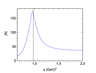
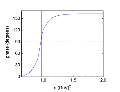
Figure 12: Results for $|A^{(0,0)}|$ - the kaon mass is artificially lowered to $M_{K}=0.4$ GeV and dynamics is implemented just by a single $f_{0}(980)$; the black vertical line indicates the actual $K\bar{K}$ threshold. left: modulus, right: phase.

We begin by considering the artificial situation in which the kaon mass is lowered to $M_{K}=0.4$ GeV, so as to allow the $f_{0}(980)$ to be above threshold. The amplitude is shown in Fig.12 and results are rather conventional. The vertical black line indicates the position of the empirical $K\bar{K}$ threshold and therefore, in actual scattering, one sees only the post-peak part of the resonance, represented by the blue curves, for scenario A, in Fig. 13. Phases in that figure follow general theorems in quantum scattering theory. In the absence of inelasticities, the phase of a generic scattering amplitude $A$ coincides with the usual phase shift $\delta$ and, at low energies the latter $\rightarrow 0$ as $q^{(2L+1)}$, where $L$ is the angular momentum and $q$ is the CM linear momentum.

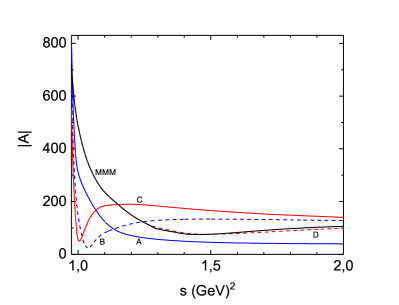
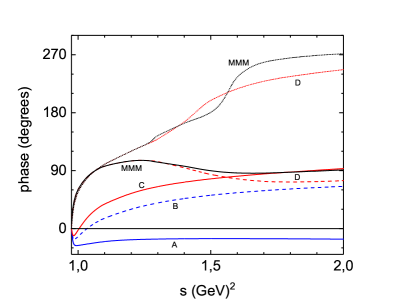
Figure 13: Results for $|A^{(0,0)}|$ - piecemeal construction of the amplitude, following steps given in table 1; the continuous blue line (A) corresponds to the tail of the $f_{0}(980)$; the dashed blue curve (B) includes the contact chiral term; the red continuous curve (C) represents the unitarized $f_{0}(980)$ and $f_{0}(1370)$ joint contributions; the dashed red curve accounts for the coupling to $\pi\pi$ intermediate states; the continuous black curve (MMM) includes coupling to $\eta\eta$ intermediate states; top: modulus; bottom: phases; the latter also includes conventional phase shifts $\delta^{(0,0)}$, indicated by the dotted curves.

Inspecting these figures, one learns that the inclusion of the chiral contact term (A $\rightarrow$ B) and the second resonance (B $\rightarrow$ C) produces a strong impact on results. The influence of the coupling to the $\pi\pi$ intermediate channel (C $\rightarrow$ D) is also rather large, especially at low energies, whereas $\eta\eta$ coupling (D $\rightarrow$ MMM) is much less important. In Fig.14 we show the inelasticity parameter $\eta$. One must have $\eta=1$ for elastic amplitudes, and we would like to draw attention to the case of scenario C, that includes two resonances and no coupled channels. In this case, the result for $\eta$ stresses that our method for dealing with multiple resonances is indeed consistent with unitarity. When the coupling to other channels is allowed, $\eta\leq 1$ and the dominance of $\pi\pi$ intermediate states becomes clear.

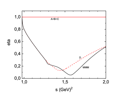
Figure 14: Results for $|A^{(0,0)}|$ inelasticities; conventions are the same as in Fig.13.

References

- (1) E.M. Aitala et al. (E791), Phys. Rev. Lett. 86 770 (2001); E.M. Aitala et al. (E791), Phys. Rev. Lett. 86 765 (2001).
- (2) E.M. Aitala et al. (E791), Phys. Rev. Lett. 89, 121801 (2002).
- (3) R. Aaij et al. [LHCb colaboration], arXiv:1712.09320, submitted to Phys. Rev. Lett. 2017 ; JHEP 03 140 (2018); arXiv:1712.08609, submitted to Eur. Phys. J. C.
- (4) D. Boito, J. -P. Dedonder, B. El-Bennich, R. Escribano, R. Kaminski, L. Lesniak and B. Loiseau, Phys. Rev. D96 11, 113003(2017).
- (5) P.C. Magalhães, M.R. Robilotta, K.S.F.F. Guimarães, T. Frederico, W.S. de Paula, I. Bediaga, A.C. dos Reis, and C.M. Maekawa, Zarnauskas,G.R.S, Phys. Rev. D84, 094001 (2011).
- (6) P.C. Magalhães and M.R. Robilotta, Phys.Rev. D 92 (2015) 094005.
- (7) K.S.F.F. Guimarães, W. de Paula, I. Bediaga, A. Delfino, T. Frederico, A. C. dos Reis and L. Tomio, Nucl. Phys. B (Proc. Suppl.) 199 (2010) 341.
- (8) Franz Niecknig and Bastian Kubis, JHEP 10, 142 (2015); Phys. Lett. B 780 (2018) 471.
- (9) S. X. Nakamura, Phys. Rev. D 93, 014005 (2016).
- (10) B. Hyams et al. Nucl. Phys. B64, 134 (1973).
- (11) Cohen, D. et al., Phys. Rev. D7, 661 (1973).
- (12) M. Albaladejo, B. Moussallam, Eur. Phys. J. C75(10), 488 (2015), 1507.04526.
- (13) M. Albaladejo and B. Moussallam, B. Eur. Phys. J. C77 no8, 508 (2017).
- (14) Ulf-G. Meiner, J.A. Oller, Nucl. Phys. A 679 671 (2001), [arXiv:hep-ph/0005253].
- (15) R. T. Aoude, P. C. Magalhães, A. C. dos Reis and M. R. Robilotta, PoS CHARM 2016 (2016) 086 [arXiv:1604.02904].
- (16) J.M. Link et al. [FOCUS Collaboration], Phys. Lett. B 681, (2009) 14;
- (17) D. R. Boito, R. Escribano, Phys. Rev. D 80, 054007 (2009); M. Diakonou and F. Diakonos, Phys. Lett. B 216, 436 (1989).
- (18) D. Aston et al., Nucl.Phys. B 296, 493 (1988).
- (19) R. Garcia-Martin, R. Kaminski, J. R. Pelaez, J. Ruiz de Elvira and F. J. Yndurain, Phys. Rev. D 83, 074004 (2011) [arXiv:1102.2183 [hep-ph]].
- (20) J.A. Oller and E. Oset, Phys. Rev. D 60, 074023 (1999); Nucl. Phys. A 620, 465 (1997); A 652, 407(E) (1999); J.R. Pelaez, J.A. Oller and E. Oset, Nucl.Phys. A675, 92C (2000); K.P. Khemchandani, A. Martinez Torres, H. Nagahiro and A. Hosaka, Phys.Rev. D88, 114016 (2013).
- (21) I.J.R. Aitchison, e-Print: arXiv:1507.02697; J.H.A. Nogueira, e-Print: arXiv:1605.03889.
- (22) G. Ecker and R. Unterdorfer, Eur.Phys.JC24, 535 (2002), Nucl.Phys.Proc.Suppl. 121, 175 (2003).
- (23) S. Weinberg, Physica A 96, 327 (1979).
- (24) J. Gasser and H. Leutwyler, Ann. Phys. 158, 142 (1984).
- (25) J. Gasser and H. Leutwyler, Nucl. Phys. B250, 465 (1985).
- (26) G. Ecker, J. Gasser, A. Pich and E. De Rafael, Nucl. Phys. B 321, 311 (1989).
- (27) G. Burdman and J.F. Donoghue, Phys. Lett. B 280, 287 (1992); M.B. Wise, Phys.Rev. D45, R2188 (1992).
- (28) C. Patrignani et al. (Particle Data Group), Chin. Phys. C, 40, 100001 (2016) and 2017 update.
- (29) R. Aaij et al. [LHCb colaboration] LHCb-CONF-2016-008, CERN-LHCb-CONF-2016-008.