Optimal Testing in the Experiment-rich Regime

Abstract

Motivated by the widespread adoption of large-scale A/B testing in industry, we propose a new experimentation framework for the setting where potential experiments are abundant (i.e., many hypotheses are available to test), and observations are costly; we refer to this as the experiment-rich regime. Such scenarios require the experimenter to internalize the opportunity cost of assigning a sample to a particular experiment. We fully characterize the optimal policy and give an algorithm to compute it. Furthermore, we develop a simple heuristic that also provides intuition for the optimal policy. We use simulations based on real data to compare both the optimal algorithm and the heuristic to other natural alternative experimental design frameworks. In particular, we discuss the paradox of power: high-powered “classical” tests can lead to highly inefficient sampling in the experiment-rich regime.

1 Introduction

In modern A/B testing (e.g., for web applications), it is not uncommon to find organizations that run hundreds or even thousands of experiments at a time (Kaufman et al., 2017; Tang et al., 2010a; Kohavi et al., 2009; Bakshy et al., 2014). Increased computational power and the ubiquity of software have made it easier to generate hypotheses and deploy experiments. Organizations typically continuously experiment using A/B testing. In particular, the space of potential experiments of interest (i.e., hypotheses being tested) is vast; e.g., testing the size, shape, font, etc., of page elements, testing different feature designs and user flows, testing different messages, etc. Artificial intelligence techniques are being deployed to help automate the design of such tests, further increasing the pace at which new experiments are designed (e.g., Sensei, Adobe’s A/B testing product, is being used in Adobe Target).

This abundance of potential experiments has led to an interesting phenomenon: despite the large numbers of visitors arriving per day at most online web applications, organizations need to constantly consider the most efficient way to allocate these visitors to experiments. For many experiments, baseline rates may be small (e.g., a low conversion rate), or more generally effect sizes may be quite small even relative to large sample sizes. For example, large organizations may be seeking relative changes in a conversion rate of $0.5$% or less, potentially necessitating millions of users allocated to a single experiment to discover a true effect. (See Tang et al. (2010a, b); Deng et al. (2013) and Azevedo et al. (2018), where these issues are discussed extensively.) Since organizations have a plethora of hypotheses of interest to test, there is a significant opportunity cost: they must constantly trade off allocation of a visitor to a current experiment against the potential allocation of this visitor to a new experiment.

In this paper, we study a benchmark model with the feature that experiments are abundant relative to the arrival rate of data; we refer to this as the experiment-rich regime. A key feature of our analysis is the impact of the opportunity cost described above: whereas much of optimal experiment design takes place in the setting of a single experiment, the experiment-rich regime fundamentally requires us to trade off the potential for discoveries across multiple experiments. Our main contribution is a complete description of an optimal discovery algorithm for our setting; the development of an effective heuristic; and an extensive data-driven simulation analysis of its performance against more classical techniques commonly applied in industrial A/B testing.

We present our model in Section 2. The formal setting we consider mimics the setting of most industrial A/B testing contexts. The experimenter receives a stream of observational units and can assign them to an infinite number of possible experiments, or alternatives, of varying quality (effect size). We consider a Bayesian setting where there is a prior over the effect size of each alternative, which is natural in a setting with an infinite number of experiments.

We focus on the objective of finding an alternative that is at least as good as a given threshold $s$ as fast as possible. In particular, we call an alternative a discovery if the posterior probability that the effect is greater than $s$ is at least $1-\alpha$, and the goal is to minimize the expected time per discovery. This is a natural criterion: good performance requires finding an alternative that is actually delivering practically significant effects (as measured by $s$). Adjusting $s$ and $\alpha$ allows the experimenter to trade off the quality and quantity of discoveries made. Note that under this criterion any optimal policy is naturally incentivized to find the “best” experiments, because the discovery criterion is easiest to be met for those alternatives.

In Section 3 we present an optimal policy for allocation of observations to experiments. Since observations arrive sequentially, the problem can be equivalently formulated as minimizing the cumulative number of observations until until a discovery is made. We characterize a dynamic programming approximation of this problem, and show this method converges to the optimal policy in an appropriate sense. We also develop a simple heuristic that approximates and provides insight into the optimal policy.

In Section 4 we use data on baseball players’ batting averages as input data for a simulation analysis of our approach. Our simulations demonstrate that our approach delivers fast discovery while controlling the rate of false discoveries; and that our heuristic approximates the optimal policy well. We also use the simulation setup to compare our method to “classical” techniques for discovery in experiments (e.g., hypothesis testing). This comparison reveals the ways in which classical methods can be inefficient in the experiment-rich regime. In particular, there is a paradox of power: efficient discovery can often lead to low power in a classical sense, and conversely high-powered classical tests can be highly inefficient in maximizing the discovery rate.

Due to space constraints, all proofs are given in the appendix.

1.1 Related work

The literature on sequential testing goes back many decades. Originally, Wald and Wolfowitz (1948) propose an optimal test, the sequential probability ratio test, or SPRT for short, for testing a simple hypothesis. Chernoff (1959) studies the asymptotics of experimentation with two hypothesis tests and how to assign observations. Lai (1988) proposes a class of Bayesian sequential tests with a composite alternative for an exponential family of distributions. For a more thorough overview of sequential testing, we refer the interested reader to Siegmund (2013), Wetherill and Glazebrook (1986), Shiryayev (1978) and Lai (1997). None of these approaches consider the opportunity cost associated with having multiple experiments.

Recently, there has been an increased interest in sequential testing due to the rise in popularity of A/B testing (Deng et al., 2017; Kaufman et al., 2017; Kharitonov et al., 2015), and the ubiquity of peeking (Johari et al., 2017; Balsubramani and Ramdas, 2016; Deng et al., 2016). A recent paper by Azevedo et al. (2018) discusses how the tails of the effect distribution affect the assignment strategy of observations to experiments and complements this work.

There is also a strong connection to the multi-armed bandit literature (Gittins et al., 2011; Bubeck and Cesa-Bianchi, 2012), especially the pure exploration problem (Bubeck et al., 2009; Jamieson et al., 2014; Russo, 2016), where the goal is to find the best arm. The case with infinitely many arms is studied by Carpentier and Valko (2015); Chaudhuri and Kalyanakrishnan (2017); Aziz et al. (2018). Locatelli et al. (2016) studies the setting of finding the set of arms (out of finitely many) above a given threshold in a fixed time horizon.

Methods to control of the false discovery rate in the sequential hypothesis setting are discussed by Foster and Stine (2007), Javanmard and Montanari (2016) and Ramdas et al. (2017). The connection between with multi-armed bandits is made by Yang et al. (2017). However, the Bayesian framework we propose does not require multiple testing corrections.

The heavy-coin problem (Chandrasekaran and Karp, 2012; Malloy et al., 2012; Jamieson et al., 2016; Lai et al., 2011) is another closely related research area. Here, a fraction of coins in a bag is considered heavy, while most are light. The goal is to find a heavy coin as quickly as possible. These approaches rely on likelihood ratios, as there are only two alternatives, and there is a connection to the CUSUM procedure (Page, 1954). The approaches mentioned above all consider the same problem as we do in this work, albeit for testing two alternatives against each other.

Optimal stopping rules have been studied extensively, often under the umbrella of the secretary problem (Freeman, 1983; Samuels, 1991). There, the focus is on comparing across alternatives.

2 Model and objective

In this section we describe the model we study and the objective of the experimenter.

Experiments. We consider a model with an infinite number of experiments, or alternatives, indexed by $i\in\{1,2,\ldots\}$. Each experiment is associated with a parameter $\mu_{i}\in M\subset\mathbb{R}$ drawn independently from a common (known) prior $\pi$ that completely characterizes the distribution of outcomes corresponding to that experiment. Throughout our analysis, the experimenter is interested in experiments with higher values of $\mu_{i}$.

Actions and outcomes. At times $t=1,2,\ldots$, the experimenter selects an alternative $I_{t}$ and observes an independent outcome $X_{t}$ drawn from a distribution $F(\mu_{I_{t}})$. Note, in particular, that opportunities for observations arrive in a sequential, streaming fashion. We also assume that observations are independent across experiments.

We assume that $F(\mu_{i})$ is described by a single parameter natural exponential family, i.e. the density for an observation can be written as:

$$f_{X}(x\mid\mu)=h(x)\exp\left(\mu S(x)-A(\mu)\right),$$ (1)

for known functions $S$, $h$, and $A$. Let $S_{t}^{i}=\sum_{t:I_{k}=i}S(X_{t})$ be the canonical sufficient statistic for experiment $i$ at time $t$. Note that in particular, this model includes the conjugate normal model with known variance and the beta-binomial model for binary outcomes.

Policies. Let $\mathcal{F}_{t}=\sigma\{X_{1},I_{1},X_{2},I_{2},\ldots,X_{t},I_{t}\}$ denote the $\sigma$-field generated. A policy is a mapping from $\mathcal{F}_{t}$ to experiments.

Discoveries. The experimenter is interested in finding discoveries, defined as follows.

Definition 1 (Discovery).

We say that alternative $i$ is a discovery at time $t$, given $s$ and $\alpha$, if

$$\mathbb{P}(\mu_{i}<s\mid\mathcal{F}_{t})<\alpha.$$ (2)

Here $s$ and $\alpha$ are parameters that capture the experimenter’s preferences, i.e., the level of aggressiveness and risk that she is willing to tolerate. (Note that this is more stringent than the related false discovery rate guarantees (Benjamini and Hochberg, 2007).)

We assume that the prior satisfies $\mathbb{P}(\mu_{i}<s\mid\emptyset)\in(\alpha,1)$ to avoid the trivial scenarios that all or none of the alternatives is a discovery before trials begin.

Objective: Minimize time to discovery. As motivated in the introduction, informally the objective is to find discoveries as fast as possible. We formalize this as follows: The goal of the experimenter is to design a policy (i.e., an algorithm to match observations to experiments) such that the number of observations until the first discovery is minimized.

In particular, define the time to first discovery $\tau$ as:

$$\tau=\min\{t:\text{there exists }i^{*}\text{ such that }\mathbb{P}(\mu_{i^{*}}<s\mid\mathcal{F}_{t})<\alpha\}.$$ (3)

Then the goal is to minimize $\mathbb{E}[\tau]$ over all policies. Given this goal, the only decision the experimenter needs to make at each point in time till the first success is whether to reject the current experiment or to continue with it.

Discussion. We conclude with two remarks regarding our model.

(1) Posterior validity. Note that at the (random) stopping time $\tau$, the posterior is computed based on the potentially adaptive matching policy used by the experimenter. The following lemma shows that when the experimenter computes the posterior and decides to stop the experiment at time $t$ when the condition $\mathbb{P}(\mu_{i^{*}}<s\mid\mathcal{F}_{t})$ is met, the decision to stop does not invalidate the discovery.

Lemma 1.

The posterior for the discovered experiment $i^{*}$ at time $\tau$ satisfies

$$\mathbb{P}(\mu_{i^{*}}<s\mid\mathcal{F}_{\tau})<\alpha$$ (4)

almost surely.

(2) Fixed cost per experiment. In some scenarios, starting a new experiment has a cost; e.g., there may be a cost to implementing a new variant, or results may need to be analyzed on a per experiment basis. We can incorporate such a cost in the objective, and our results and approach generalize accordingly. Formally, let $c$ be the cost of starting a new experiment, and let $m_{t}=|\{i:\exists t^{\prime}\leq t:I_{t^{\prime}}=i\}|$ be the cumulative number of matched experiments up to time $t$. We can include the per experiment cost by considering instead the problem of minimizing $\mathbb{E}[\tau+cm_{\tau}]$.

3 Optimal policy

In this section, we characterize the structure of the optimal policy, show that it can be approximated arbitrarily well by considering a truncated problem, and give an algorithm to compute the optimal policy of the truncated problem. Finally, we present a simple heuristic that approximates the optimal policy remarkably well.

3.1 Sequential policies

We start with a key structural result that simplifies the search for an optimal policy. The following lemma shows that we can focus on policies that only consider experiments sequentially, in the sense that once a new experiment is being allocated observations, no previous experiment will ever again receive observations.

Lemma 2.

There exists an optimal policy such that $I_{t+1}\geq I_{t}$ for all $t$ almost surely.

This result hinges on three aspects of our model: experiments are independent of each other, with identically distributed effects $\mu_{i}$; there are an infinite number of experiments available; and observations arrive in an infinite stream. As a consequence, all experiments are a priori equally viable, and a posteriori once the experimenter has determined to stop allocating observations to an experiment, she need never consider it again.

Note in particular that this lemma also reveals that any optimal policy for the first discovery also straightforwardly minimizes the expected time until the $k$’th discovery, for any $k$.

3.2 Reformulating the optimization problem

Based on Lemma 2, we can reformulate and simplify the optimization problem faced by the experimenter as a sequential decision problem, where the only choice is whether or not to continue testing the current experiment.

We abuse notation to describe this new perspective. Let $\mu$ denote the effect size of the current experiment. In particular, let $X_{n}$ be the $n$’th observation; let $\mathcal{F}_{n}$ be the $\sigma$-field generated by observations of the current experiment $(X_{1},\ldots,X_{n})$. Let $S_{n}=\sum_{k=1}^{n}S(X_{k})$ denote the canonical sufficient statistic at state $n$. The state of the sequential decision problem is $(n,S_{n})$, the number of observations and the sufficient statistic of the current experiment.

If $(n,S_{n})$ has the property that $\mathbb{P}(\mu<s|S_{n})<\alpha$, then a discovery has been found and so the process stops. The following lemma shows that this discovery criterion induces an acceptance region on the sufficient statistic $S_{n}$, i.e., a sequence of thresholds $a_{n}$ such the current experiment is a discovery when $S_{n}\geq a_{n}$.

Lemma 3.

There exists a sequence $\{a_{n}\}_{n=1}^{\infty}$ such that $\mathbb{P}(\mu<s\mid S_{n})<\alpha$ if and only if $S_{n}>a_{n}$.

If $S_{n}<a_{n}$, then the experimenter can make one of two decisions:

1. Continue (i.e., collect one additional observation on the current experiment); or

2. Reject (i.e., quit the current experiment and collect the first observation of a new experiment).

If Continue is chosen, the state updates to $(n+1,S_{n+1})$. If Reject is chosen, the state changes to $(1,S_{1})$ (where $S_{1}$ is an independent draw of the sufficient statistic after the first observation); and in either case, the process continues.

The goal of the experimenter is to minimize the expected time until the observation process stops, i.e., until a discovery is found. Let $V(n,S_{n})$ be this minimum, starting from state $(n,S_{n})$. Then the Bellman equation for this process is as follows:

$$V(n,S_{n}) =0,\ \ S_{n}\geq a_{n};$$ (5)

$$V(n,S_{n}) =1+\min\left\{\mathbb{E}[V(n+1,S_{n+1})|S_{n}],\mathbb{E}[V(1,S_{1})]\right\},\ \ S_{n}\leq a_{n}\ \ n\geq 1.$$ (6)

The first line corresponds to the case where $S_{n}$ is in the acceptance region, i.e., the process stops. In the second line, we consider two possibilities: continuing incurs a unit cost for the current observation, plus the expected cost from the state $(n+1,S_{n+1})$; rejecting resets the state with no cost incurred. The optimal choice is found by minimizing between these alternatives. The expected number of samples $T^{*}$ till a discovery satisfies $T^{*}=1+\mathbb{E}[V(1,S_{1})]$.

3.3 Characterizing the optimal policy

The following theorem shows that an optimal policy for the dynamic programming problem (5)-(6) can be expressed using a sequence of rejection thresholds on the sufficient statistic. That is, for each $n$ there is an $r_{n}$ such that it is optimal to Continue if $S_{n}\geq r_{n}$, and to Reject if $S_{n}<r_{n}$.

Theorem 4.

There exists an optimal policy for (5)-(6) described by a sequence of rejection thresholds $\{r_{n}\}_{n=1}^{\infty}$ such that, after $n$ observations, Reject is declared if $S_{n}<r_{n}$, Continue is declared if $r_{n}\leq S_{n}\leq a_{n}$, and the process stops with a discovery if $S_{n}>a_{n}$.

The remainder of the section is devoted to computing the optimal sequence of rejection thresholds.

3.4 Approximating the optimal policy via truncation

In order to compute an optimal policy, we consider a truncated problem. This problem is identical in every respect to the problem in Section 3.2, except that we consider only policies that must choose Reject after $k$ observations. We refer to this as the $k$-truncated problem.

Let $V_{k}(n,S_{n})$ denote the minimum expected cumulative time to discovery for the $k$-truncated problem, starting from state $(n,S_{n})$. The Bellman equation is nearly identical to (5)-(6), except that now $V_{k}(k,S_{k})=1+\mathbb{E}[V_{k}(1,S_{1})],S_{k}\leq a_{k}$, and we add the additional constraint that $n<k$ to (6). We have the following proposition.

Theorem 5.

There exists an optimal policy for the $k$-truncated problem described by a sequence of rejection thresholds $\{r_{n}^{k}\}_{n=1}^{\infty}$ such that, after $n$ observations, Reject is declared if $S_{n}<r_{n}^{k}$, Continue is declared if $r_{n}^{k}\leq S_{n}\leq a_{n}$, and Accept is declared is if $S_{n}>a_{n}$.

Further, let $T_{k}^{*}=\mathbb{E}[V_{k}(1,S_{1})]+1$ be the optimal expected number of observations until a discovery is made. Then for each $n$, $r_{n}^{k}\to r_{n}$ as $k\to\infty$; and $T_{k}^{*}\to T^{*}$ as $k\to\infty$.

3.5 Computing the truncated optimal policy

The truncated horizon brings us closer to computing an optimal policy, but it is still an infinite horizon dynamic programming problem. In this section we show instead that we can compute the truncated optimal policy by iteratively solving a single-experiment truncated problem with a fixed rejection cost $\kappa$. Let $W_{k}(n,S_{n}|\kappa)$ be the optimal expected cost for this problem starting from state $(n,S_{n})$. We have the following Bellman equation.

$$W_{k}(n,S_{n}|\kappa) =0,\ \ S_{n}>a_{n};$$ (7)

$$W_{k}(k,S_{k}|\kappa) =\kappa,\ \ S_{k}\leq a_{k};$$ (8)

$$W_{k}(n,S_{n}|\kappa) =1+\min\left\{\mathbb{E}[W_{k}(n+1,S_{n+1}|\kappa)|S_{n}],\kappa\right\},\ \ n<k,S_{n}\leq a_{n}.$$ (9)

For any terminal cost $\kappa$, this dynamic programming problem is easily solved using backward induction to find the rejection boundaries. The following theorem shows how we can use this solution to find an optimal policy to the truncated problem.

Theorem 6.

If $\kappa=T_{k}^{*}$, then the optimal policy for (7)-(9) with rejection thresholds $\overline{r}_{n}^{k}$ found by backward induction satisfies $\overline{r}_{n}^{k}=r_{n}^{k}$ for all $n\leq k$. Furthermore, let $f(\kappa)=1+\mathbb{E}[W_{k}(1,S_{1}|\kappa)]$ be the optimal cost. Then if $\kappa>T_{k}^{*}$, $f(\kappa)<\kappa$, and if $\kappa<T_{k}^{*}$, then $f(\kappa)>\kappa$.

Thus, to find approximately optimal rejection thresholds, select $k$ suitably large, and start with an arbitrary $\kappa$. Then iteratively compute the corresponding thresholds $\overline{r}_{n}^{k}$ and the cost $f(\kappa)$, using bisection to converge on $T_{k}^{*}$, and thus the corresponding optimal thresholds.

We note that the same program we have outlined in this section can be used to compute an optimal policy with a per experiment fixed cost $c$, by using rejection cost $\kappa+c$ instead of $\kappa$. Empirically, this leads to only slightly lower rejection thresholds; due to space constraints, we omit the details.

3.6 Heuristic approximation

We have seen that the optimal policy is easy to approximate by solving dynamic programs iteratively. However, this does not give us direct insight into the structure of the solution, and in certain cases a quick rule-of-thumb that provides an approximate policy might be all that is required. In this section, we show that there exists a simple heuristic that performs remarkably well.

The approximate rejection boundary at time $n$ is found as follows. Let $\hat{\mu}$ be the MAP estimate of $\mu$ for sufficient statistic $S_{n+T^{*}}=a_{n+T^{*}}$. Then reject the current experiment if $S_{n}$ is not plausible under $\hat{\mu}$. That is, the heuristic boundary $\overline{r}_{n}$ is, for a suitably chosen $\beta$,

$$\mathbb{P}(S_{n}\leq\overline{r}_{n}\mid\mu=\hat{\mu})=\beta.$$ (10)

Of course, this heuristic is not practical as is, as in general we do not know $T^{*}$ unless we compute the optimal policy. But often $a_{n+t}$ varies only little in $t$ so a reasonable approximate choice $T_{h}$ is sufficient. In Figure 1 we plot the discovery and rejection boundaries, along with the heuristic outlined above (with $T_{h}=T^{*}$), for the normal and Bernoulli models.

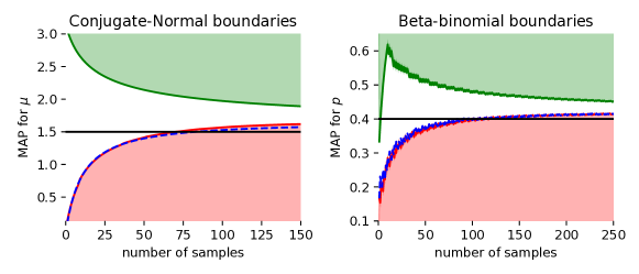
Figure 1: Acceptance and rejection regions for the conjugate Normal and the Beta-Binomial models. The dashed blue line gives the heuristic rejection boundary, while the red line corresponds to the optimal rejection thresholds. Note that the boundaries are shown in terms of the MAP estimate.

The heuristic and optimal policies clearly exhibit aggressive rejection regions, cf. Figure 1. THe interpretation is as follows: to continue sampling from the current experiment, we do not just want its quality to be $s$, but substantially better than $s$, since $a_{n}>s$ for all $n$. If not, it would take too many additional observations to verify the discovery.

4 Case study: baseball

We now empirically analyze our testing framework based on a simulation with baseball data. First, we demonstrate empirically that the proposed algorithm leads to fast discoveries, and behaves differently from traditional testing approaches. Second, we show that the rule-of-thumb heuristic performance is close to that of the optimal policy.

Data We use the baseball dataset with pitching and hitting statistics from 1871 through 2016 from the Lahman R package. The number of At Bats (AB) and Hits (H) is collected for each player, and we are interested in finding players with a high batting average, defined as $b_{i}=\text{Hits}_{i}/\text{At Bats}_{i}$. We consider players with at least $200$ At Bats, which leaves a total of 5721 players, with a mean of about 2300 At Bats. In the top left of Figure 2, we plot the histogram of batting averages, along with an approximation by a beta distribution (fit via method of moments). We note that these fit the data reasonably well, but not perfectly. This discrepancy helps us evaluate the robustness to a misspecified prior.

Simulation setup To construct the testing problem, we view the batters as alternatives, with empirical batting average $b_{i}$ of batter $i$ treated as ground truth. We want to find alternatives with $b_{i}>s$. We draw a Bernoulli sample of mean $b_{i}$ to simulate an observation from alternative $i$. These samples are then used to test whether $b_{i}>s$. We set $\alpha=0.05$, and vary $s$ between $0.25$ and $0.32$. For each simulation, we iterate through each batter and repeat it 1000 times to reduce variance. This allows us to compare methods fairly, ensuring that each procedure is run on exactly the same test cases.

4.1 Benchmarks

To assess performance, we compare several testing procedures. Note that the non-traditional setup of our testing framework does not allow for easy comparison with other methods, in particular frequentist approaches, as they give different guarantees. Thus, we restrict attention to Bayesian methods that provide the same error guarantee. All of the benchmarks use the same beta prior computed above.

Optimal policy

First we study the optimal policy based on the beta-binomial model, computed using the bisection and backward induction approach in Section 3.5, where we truncate after $k=5000$ samples.

Heuristic policy

Next, we include the heuristic rejection thresholds that approximate the optimal policy for truncation $k=5000$ samples. The heuristic policy requires setting two parameters: $T_{h}$, i.e., how far to look into the future to find the acceptance boundary, which is ideally set close to $T^{*}$; and the rejection region $\beta$. To demonstrate the the insensitivity to $T^{*}$, we use $T_{h}=2000$ and $\beta=0.2$ for all simulations. (Note that $T^{*}$ varies dramatically as we change the threshold $s$.

Fixed sample size test

Our next benchmark is a simple fixed sample size test. For each experiment, we gather $N$ observations, and claim a discovery if $P(\mu_{i}<s\mid Y_{i})<\alpha$ where $Y_{i}$ is the number of Hits of alternative (batter) $i$. We focus our attention on using $N=1000$ samples per test, as this seems to perform best when compared to other sample sizes, but any differences are immaterial for our conclusions.

Fixed sample size test with early stopping

This benchmark is similar to the fixed sample size test, except that we stop the experiment early if the discovery criterion is met. Thus, we can quantify the gains from being able to discover early.

Bayesian sequential test

Now we consider a sequential test that also rejects early. In particular, we reject the current experiment if $\mathbb{P}(b_{i}>s\mid\boldsymbol{\mathrm{S}}_{t}^{i})<\beta.$ We also reject an alternative after $4000$ samples. This approach also requires careful tuning of $\beta$. In particular, if $\beta$ is too large, say larger than the prior probability $\mathbb{P}_{0}(b_{i}>s)$, then the test is too aggressive and rejects all alternatives outright. Instead, we found empirically that setting $\beta=0.9\mathbb{P}_{0}(b_{i}>s)$ leads to good performance across all values of $s$.

4.2 Results

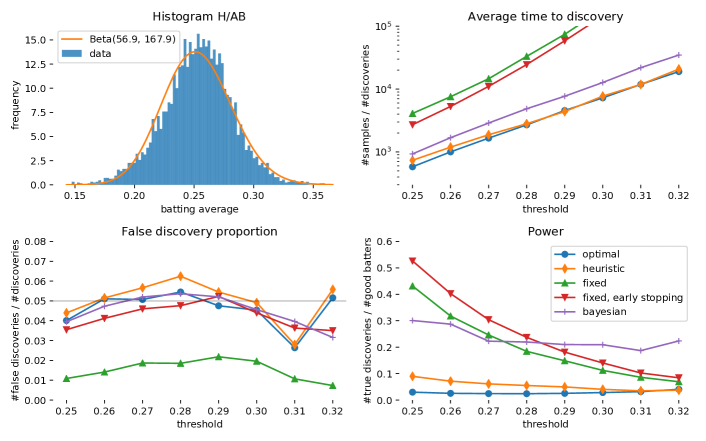
Figure 2: Top left: histogram of batting averages. Top right: Efficacy of of algorithms. Bottom left: Plot the false discovery proportion across thresholds. Bottom right: Plot of the empirical power of algorithms. Note the paradox of power effect: the most efficient algorithms have low power.

Average time to discovery

The average number of observations until a discovery is shown in the top right plot of Figure 2. As expected, the fixed sample test performs worst. Early stopping leads to slightly better performance, but this method is still not effective as most of the gains come from early rejection. The Bayesian sequential test demonstrates this effect and shows substantial gains over the fixed tests. The heuristic policy, despite lack of parameter tuning, performs very well, essentially matching the performance of the optimal algorithm for most thresholds.

False discovery proportion and robustness

Next, we compare the false discovery proportion (FDP) (Benjamini and Hochberg, 2007), i.e., the fraction of discoveries that in fact had true $b_{i}<s$. If the prior is correctly specified, the methods we consider satisfy $\mathbb{E}(\textup{FDP})\leq\alpha$. Indeed, we observe that the guarantee holds for most thresholds and algorithms in the bottom left plot of Figure 2. There is some minor exceedance of the FDP for thresholds around $s\approx 0.28$, which can be explained by the fact that the prior does not fit the empirical batting averages perfectly. Since there are few rejections for thresholds beyond $s=0.3$, the FDP estimate has higher variance in that regime. Across all simulations, the optimal policy has an FDP of $0.048<\alpha$. Finally, we see that the lack of early stopping makes the fixed test rather conservative.

The paradox of power

Finally, we compare power, i.e., the fraction of alternatives $i$ with $b_{i}>s$ that are declared a discovery. Power comparisons across the algorithms are plotted in the bottom right of Figure 2. The most surprising insight from the simulations is the paradox of power. Algorithms that are effective have very low power. This is counter-intuitive: how can algorithms that make many discoveries have only a small chance of picking up true effects? The main driver of good performance for an algorithm is the ability to quickly reject unpromising alternatives. Some unpromising alternatives are “barely winners”: i.e., $b_{i}$ is only slightly above $s$. In the experiment-rich regime, such alternatives should be rejected quickly, because it takes too many observations to get enough concentration around the posterior to claim a discovery. This effect leads to low power, but fast discoveries.

Characteristics of the optimal policy

We consider the outcomes of individual tests for the optimal algorithm ($s=0.27$) in Figure 3. The average number of samples for rejected alternatives is very small while it is much larger for discovered alternatives. We also note the concave shape for the discovered alternatives, that seems to peek around $0.285$. When the batting average is larger, the algorithm is able to detect the effect with fewer samples, and when the batting average is lower, there are a few lucky streaks that lead to a (false) discovery.

The probability of discovery is low across all batting averages, but increases sharply beyond a batting average of $0.28$, rather than around $s=0.27$. As noted before, the optimal policy tries to avoid effects that are close to the threshold.

Finally, the MAP estimates for the batting averages of discovered batters. It illustrates a known but important fact that the parameter of discovered alternatives are quite poor. If estimation of effects is important, the experimenter ought to obtain more samples for the discovered alternatives.

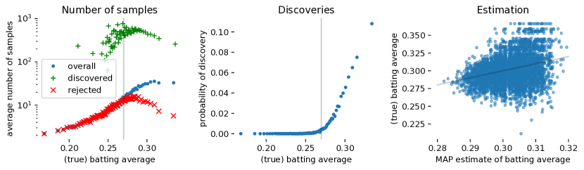
Figure 3: Analysis of optimal policy. The left plot shows average number of samples for rejections and discoveries. The center plot shows the fraction of discoveries. The right plot shows MAP estimates of effect sizes.

5 Conclusion

We consider an experimentation setting where observations are costly, and there is an abundance of possible experiments to run — an increasingly prevalent scenario as the world is becoming more data-driven. Based on backward induction, we can compute an approximately optimal algorithm that allocates observations to experiments such that the time to a discovery is minimized. Simulations validate the efficacy of our approach, and also reveal discuss the paradox of power: there is a tension between high-powered tests, and being efficient with observations.

Our paradigm has several additional practical benefits. First, we can leverage knowledge across experiments through the prior. Second, adaptive matching of observations to experiments does not preclude valid inference, and thus outcomes can thus continuously be monitored. Finally, the framework also provides an easy “user interface”: it directly incorporates the desired effect size, and leads to guarantees that are easy to explain to non-experts.

Further directions

The framework assumes there is a common prior among alternatives, and this allows us to view every rejection as a renewal. If experiments have different priors, then the order at which experiments are chosen matters. This is also true when the costs of observations or starting experiments differ across experiments.

Furthermore, we assume the prior is known. The experimenter can take an empirical Bayes approach similar to our simulations before starting the experiments, but data gathered while the optimal policy is running distorts estimates of the prior.

We briefly touched upon the independence assumption across observations of a single experiment, and showed that for baseball data this does not lead to problems, but in other use cases time variation, e.g. novelty effects, might play a bigger role and need to be encoded into the framework. One way to incorporate such effects, along with suitably chose covariates that can reduce the variance of testing and thereby improving the time till discoveries are Bayesian generalized linear models.

Finally, we assume that experiments are independent. In certain settings the results of one experiment can affect future experiments, or there might be correlations between outcomes of experiments. Incorporating these effects is non-trivial and beyond the scope of this work.

6 Acknowledgements

The authors would like to thank Johan Ugander, David Walsh, Andrea Locatelli, and Carlos Riquelme for their suggestions and feedback. This work was supported by the Stanford TomKat Center, and by the National Science Foundation under Grant No. CNS-1544548 and CNS-1343253. Any opinions, findings, and conclusions or recommendations expressed in this material are those of the author(s) and do not necessarily reflect the views of the National Science Foundation.

Appendix A Proofs

A.1 Proofs from Section 2

Proof of Lemma 1.

The result relies on $\tau$ being a stopping time. Recall that $i^{*}$ indicates the discovered experiment. Then we find

$$\mathbb{P}(\mu_{i^{*}}<s\mid\mathcal{F}_{\tau}) =\sum_{t=1}^{\infty}\mathbb{P}(\mu_{i}^{*}<s\mid\mathcal{F}_{\tau}\cap\{\tau=t\})\mathbb{P}(\tau=t)$$

$$=\sum_{t=1}^{\infty}\mathbb{P}(\mu_{i}^{*}<s\mid\mathcal{F}_{t})\mathbb{P}(\tau=t)$$

$$\leq\alpha\sum_{t=1}^{\infty}\mathbb{P}(\tau=t)=\alpha$$

where we use that $F\in\mathcal{F}_{\tau}$ if $F\cap\{\tau=t\}\in\mathcal{F}_{t}$, and thus $\mathcal{F}_{\tau}=\mathcal{F}_{t}$ if $\tau=t$ [Williams, 1991][p.219]. ∎

Proof of Lemma 2.

Note that due to independence we can assume without loss of generality that the index of the arm corresponds to the order in which alternatives are first considered. Thus the result follows if we show that for any $t$, action $I_{t}<I_{t-1}$ cannot be strictly better than $I_{t}=I_{t+1}$. Assume to the contrary that $I_{t}=y$ is optimal (and strictly better than $I_{t}=I_{t-1}+1$ for some $y<I_{t}$. Consider the last time alternative $y$ was selected: $t^{\prime}=\max\{k<t:I_{k}=y\}$. At that time it was at least as good to consider a new alternative, and subsequently the posterior for alternative $y$ has not changed due to independence. Due to the infinite time horizon, it is thus at least as good to consider a new alternative. ∎

A.2 Proofs from Section 3

Proof of Lemma 3.

Let $n\geq 1$. We can rewrite the discovery criterion as

$$\mathbb{P}(\mu<s\mid S_{n}=t) =\frac{\int_{-\infty}^{s}\prod_{i=1}^{n}h(X_{i})\exp\left(\mu S(X_{i})-A(\mu)\right)d\pi(\mu)}{\int_{-\infty}^{\infty}\prod_{i=1}^{n}h(X_{i})\exp\left(\mu S(X_{i})-A(\mu)\right)d\pi(\mu)}$$ (11)

$$=\frac{\int_{-\infty}^{s}\exp\left(\mu S_{n}-nA(\mu)\right)d\pi(\mu)}{\int_{-\infty}^{\infty}\exp\left(\mu S_{n}-nA(\mu)\right)d\pi(\mu)}$$ (12)

$$=\frac{\int_{-\infty}^{s}\exp\left(\mu t-nA(\mu)\right)d\pi(\mu)}{\int_{-\infty}^{\infty}\exp\left(\mu t-nA(\mu)\right)d\pi(\mu)}$$ (13)

We show that this is decreasing in $t$.

Now take the logarithm and the derivative with respect to $t$ to obtain Find expression

$$\frac{d}{dt}\log(\mathbb{P}(\mu<s\mid S_{n}=t)) =\frac{\int_{-\infty}^{s}\mu\exp(\mu t-nA(\mu))d\pi(\mu)}{\int_{-\infty}^{s}\exp(\mu t-nA(\mu))d\pi(\mu)}$$ (14)

$$\quad-\frac{\int_{-\infty}^{\infty}\mu\exp(\mu t-nA(\mu))d\pi(\mu)}{\int_{-\infty}^{\infty}\exp(\mu t-nA(\mu))d\pi(\mu)}$$ (15)

$$=\mathbb{E}_{f_{t}}(\mu\mid\mu<s)-\mathbb{E}_{f_{t}}(\mu)<0$$ (16)

where the expectations in the last line is taken with respect to the distribution with density

$$f_{t}(\mu)=\frac{\exp(\mu t-nA(\mu))d\pi(\mu)}{\int_{-\infty}^{s}\exp(\mu t-nA(\mu))d\pi(\mu)}\\$$ (17)

Note that the last inequality holds, because, in general

$$\mathbb{E}(\theta)=\mathbb{E}(\theta\mid\theta<s)\mathbb{P}(\theta<s)+\mathbb{E}(\theta\mid\theta\geq s)\mathbb{P}(\theta\geq s)\\ >\mathbb{E}(\theta\mid\theta<s)\mathbb{P}(\theta<s)+s\mathbb{P}(\theta\geq s)>\mathbb{E}(\theta|\theta<s)$$ (18)

Now the lemma follows: if $\mathbb{P}(\mu<s\mid S_{n}=t)<\alpha$, then $\mathbb{P}(\mu<s\mid S_{n}=t^{\prime})<\alpha$ for all $t^{\prime}>t$, and similarly if if $\mathbb{P}(\mu<s\mid S_{n}=t)>\alpha$, then $\mathbb{P}(\mu<s\mid S_{n}=t^{\prime})>\alpha$ for all $t^{\prime}<t$. ∎

To prove the theorems in Section 3 we use the following lemmas, which are proven at the end of this section.

Lemma 7.

The optimal policy for the truncated problem can be characterized by a rejection threshold. That is, the optimal policy rejects the current experiment if $S_{n}<r^{k}_{n}$ for a sequence $r^{k}_{n}$, and collects another observation for the current experiment otherwise, until a discovery is made.

Write $T_{k}$ for the expected number of observations required for a discovery for the optimal policy of the truncated problem. Then we can show that both $T_{k}$ and $r_{n}^{k}$ converge.

Lemma 8.

Both $T_{k}$ and $r_{n}^{k}$ converge as $k\to\infty$.

Proof of Theorem 4.

Lemma 7 shows that the truncated problem has an optimal policy that has the form of a threshold. Next, lemma 8 shows that both the thresholds and the optimal cost converge.

Recall $T^{*}=\lim_{k\to\infty}T_{k}^{*}$ and $r_{n}=\lim_{k\to\infty}r_{n}^{k}$. Now we show that limiting policy $r_{n}$ with corresponding cost $T^{*}$ is optimal.

Suppose there exists an $\varepsilon>0$ and a policy $\overline{\phi}$ with cost $\overline{T}$ such that $\overline{T}=T^{*}-\varepsilon$. Consider a policy with cost $\overline{T}<T^{*}$. Let $\overline{\tau}$ be the stopping time of this policy. We consider the truncated version of this policy, and show that it cannot be much worse. On the other hand, this truncated policy has a cost larger than $T^{*}$. The $k$-truncated policy, denoted by $\overline{\phi}_{k}$ rejects the current alternative after $k$ samples, but is otherwise identical to $\overline{\phi}$. Let $\overline{\tau}$ and $\overline{\tau}_{k}$ be the stopping times corresponding to $\overline{\phi}$ and $\overline{\phi}_{k}$. Trivially, we have $\overline{T}=\sum_{k=1}^{\infty}\mathbb{P}(\overline{\tau}\geq k)$. Because $\overline{T}$ is finite, $\mathbb{P}(\overline{\tau}\geq k)=O((k\log k)^{-1})$. Because $\overline{\phi}$ and $\overline{\phi}_{k}$ are identical up to $k$ observations, it follows that if $\overline{\tau}<k$, then $\overline{\tau}_{k}<k$, and thus we find that

$$\mathbb{E}(\overline{\tau}_{k}) =\mathbb{P}(\overline{\tau}>k)\mathbb{E}(\overline{\tau}_{k}\mid\overline{\tau}>k)+\mathbb{E}(\overline{\tau}{\mathbb{I}}(\overline{\tau}\leq k))$$

$$\leq\mathbb{P}(\overline{\tau}>k)(k+\mathbb{E}(\overline{\tau}_{k}))+\mathbb{E}(\overline{\tau}{\mathbb{I}}(\overline{\tau}\leq k))$$

Thus, it follows that

$$\mathbb{E}(\overline{\tau}_{k})\leq\frac{k\mathbb{P}(\overline{\tau}>k)}{1-\mathbb{P}(\overline{\tau}>k)}+\frac{\overline{T}}{1-\mathbb{P}(\tau>k)}.$$ (19)

Since $\mathbb{P}(\overline{\tau}>k)=O((k\log k)^{-1})$, $\mathbb{E}(\overline{\tau}_{k})\to\overline{T}$ as $k\to\infty$.

However, $T^{*}\leq\mathbb{E}(\overline{\tau}_{k})$ for all $k$, and thus $T^{*}\leq\lim_{k\to\infty}\mathbb{E}(\overline{\tau}_{k})=\overline{T}$, which is a contradiction. ∎

Proof of Theorem 5.

This is a direct consequence of lemmas 7 and 8. ∎

Proof of Theorem 6.

Let $\tau_{r}$ denote the (random) hitting time of the boundary of the first alternative

$$\tau_{r}=\min\{n:S_{n}\geq a_{n}\text{ or }S_{n}<r_{n}\}$$ (20)

under rejection boundary $r=\{r_{n}\}_{i=1}^{k}$. Furthermore, let $q_{r}=\mathbb{P}(S_{\tau}<r_{\tau})$ denote the rejection probability. Now note that $f(\kappa)=\min_{r}\mathbb{E}(\tau_{r})+\kappa q_{r}$ Note that we can solve this minimization problem using backward induction, since the time horizon is fixed ($k$). First, we show that $f$ has a unique fixed point which is equal to $T_{k}^{*}$.

Note that we have

$$T_{r}=\mathbb{E}(\tau_{r})+T_{r}q_{r}$$ (21)

By definition, $T_{k}^{*}$ minimizes $\min_{r}\mathbb{E}(\tau_{r})+T_{k}^{*}q_{r}$, thus, it follows immediately that $T_{k}^{*}$ is a fixed point of $f$.

Next, we show that $f(\kappa)>\kappa$ for each $\kappa<T_{k}^{*}$ and $f(\kappa)<\kappa$ for each $\kappa>T_{k}^{*}$.

First, fix $\kappa<T_{k}^{*}$. Suppose that $f(\kappa)\leq\kappa$. Thus, there exists $r^{\prime}$ such that $\mathbb{E}(\tau_{r^{\prime}})+\kappa q_{r^{\prime}}\leq\kappa$. Thus, $\kappa\geq\frac{\mathbb{E}(\tau_{r^{\prime}})}{1-q_{r^{\prime}}}=T_{r^{\prime}}$, where the last equality follows from (21). This, along with $\kappa<T_{k}^{*}$ implies that $T_{r^{\prime}}<T_{k}^{*}$, a contradiction. Thus, we must have $f(\kappa)>\kappa$.

Finally, fix $\kappa>T^{*}$. We know that

$$T^{*}=\mathbb{E}(\tau_{r^{*}})+T_{k}^{*}q_{r^{*}}<\mathbb{E}(\tau_{r^{*}})+\kappa q_{r^{*}}.$$ (22)

Thus, there exists $r$ (equal to $r^{*}$) such that $\mathbb{E}[\tau_{r}]+\kappa q_{r}<\kappa$. Thus, $f(\kappa)<\kappa$. ∎

A.3 Proofs of lemmas

Proof of Lemma 7.

Based on Lemma 2, there exists a policy that can be characterized by a sequence of three sets

• Discover if $S_{n}\in A_{n}$, the experiment is a discovery

• Continue if $S_{n}\in D_{n}$, and

• Reject if $S_{n}\in R_{n}$

Now note that $R^{k}_{n}$ is a threshold region for $n\geq k$ by definition. Assume $R^{k}_{m}=(-\infty,r_{m}^{k}]$ for all $m>n$. Further, from the Bellman equation for the truncated problem, it is clear that the optimal solution rejects the current experiment at the time $n$ if

$$\mathbb{E}[V_{k}(n+1,S_{n+1})\mid S_{n}]>\mathbb{E}[V_{k}(1,S_{1})]=T_{k}^{*}-1.$$ (23)

Note that

$$\mathbb{E}[V_{k}(n+1,S_{n+1})\mid S_{n}=x]=\int_{y\in D_{n+1}}V_{k}(n+1,y)f(S_{n+1}=y\mid S_{n}=x)dy\\ +T_{k}^{*}\mathbb{P}(S_{n+1}<r_{n+1}\mid S_{n}=x)$$ (24)

Then for $n$ we note that $\mathbb{E}[V_{k}(n+1,S_{n+1})\mid S_{n}=x]$ is decreasing in $x$. This follows since $V_{k}(n+1,y)<T_{k}^{*}$ for all $y\in D_{n+1}=[r_{n+1},a_{n+1}]$, as for such $y$ it is better to continue than to reject. Furthermore, arguing along the lines of the proof of Lemma 3, $\mathbb{P}(S_{n+1}<r_{n+1}\mid S_{n}=x)$ is decreasing in $x$. This implies we can write $R_{n}^{k}=(-\infty,r_{n}^{k}]$ for some $r_{n}^{k}$. ∎

Proof of Lemma 8.

Due to increased degrees of freedom, it follows that $T_{k}^{*}$ is decreasing. Since $T_{k}^{*}$ is bounded below by $0$, $T_{k}^{n}$ converges. Let $T^{*}=\lim_{k}T_{k}^{*}$.

Next, we show that $r_{n}^{k}$ is decreasing in $k$: Clearly, $r_{k}^{k+1}\leq r_{k}^{k}$. Now suppose $r_{n+1}^{k+1}\leq r_{n+1}^{k}$, then $r_{n}^{k+1}\leq r_{n}^{k}$, which follows from the fact that $\mathbb{E}[V_{k}(n+1,S_{n+1})\mid S_{n}=r_{n}^{k}]+1=T_{k}^{*}$, and $T_{k}^{*}$ is decreasing in $k$. It remains to show that $r_{n}^{k}$ is bounded.

We construct a lower bound on $r_{n}^{k}$, for large $k$, as follows. Let $\varepsilon=\frac{1}{2T^{*}}$ and let $x$ be such that $\mathbb{P}(\exists m>n\text{ s.t. }S_{m}>a_{m}\mid S_{n}=x)<\varepsilon$, by choosing $x$ sufficiently small. Then we note that the cost for obtaining another sample is at least $1+(1-\varepsilon)T_{k}^{*}\geq 1+(1-\varepsilon)T^{*}=T^{*}+1/2$. However, if the experimenter rejects the current alternative now, the cost is $T_{k}^{*}$. Thus, if we can show that there exists a $K$ such that for all $k>K$, $T_{k}^{*}<T^{*}+1/2$, then $x$ is a lower bound on $r_{n}^{k}$ for all $k>K$. But above we have shown that $T_{k}^{*}\to T^{*}$, hence such $K$ exists. This implies that $r_{n}^{k}$ converges as $k\to\infty$. ∎

References

- Azevedo et al. [2018] Eduardo M Azevedo, Alex Deng, Jose Montiel Olea, Justin M Rao, and E Glen Weyl. A/b testing. In Proceedings of the Nineteenth ACM Conference on Economics and Computation. ACM, 2018.
- Aziz et al. [2018] Maryam Aziz, Jesse Anderton, Emilie Kaufmann, and Javed A. Aslam. Pure exploration in infinitely-armed bandit models with fixed-confidence. In ALT, 2018.
- Bakshy et al. [2014] Eytan Bakshy, Dean Eckles, and Michael S Bernstein. Designing and deploying online field experiments. In Proceedings of the 23rd international conference on World wide web, pages 283–292. ACM, 2014.
- Balsubramani and Ramdas [2016] Akshay Balsubramani and Aaditya Ramdas. Sequential nonparametric testing with the law of the iterated logarithm. CoRR, abs/1506.03486, 2016.
- Benjamini and Hochberg [2007] Author Yoav Benjamini and Yosef Hochberg. Controlling the false discovery rate: A practical and powerful approach to multiple testing. 2007.
- Bubeck and Cesa-Bianchi [2012] Sébastien Bubeck and Nicolò Cesa-Bianchi. Regret analysis of stochastic and nonstochastic multi-armed bandit problems. Foundations and Trends in Machine Learning, 5:1–122, 2012.
- Bubeck et al. [2009] Sébastien Bubeck, Rémi Munos, and Gilles Stoltz. Pure exploration in multi-armed bandits problems. In ALT, 2009.
- Carpentier and Valko [2015] Alexandra Carpentier and Michal Valko. Simple regret for infinitely many armed bandits. In ICML, 2015.
- Chandrasekaran and Karp [2012] Karthekeyan Chandrasekaran and Richard M. Karp. Finding the most biased coin with fewest flips. CoRR, abs/1202.3639, 2012.
- Chaudhuri and Kalyanakrishnan [2017] Arghya Roy Chaudhuri and Shivaram Kalyanakrishnan. Pac identification of a bandit arm relative to a reward quantile. In AAAI, pages 1777–1783, 2017.
- Chernoff [1959] Herman Chernoff. Sequential design of experiments. The Annals of Mathematical Statistics, 30(3):755–770, 1959.
- Deng et al. [2013] Alex Deng, Ya Xu, Ron Kohavi, and Toby Walker. Improving the sensitivity of online controlled experiments by utilizing pre-experiment data. In Proceedings of the sixth ACM international conference on Web search and data mining, pages 123–132. ACM, 2013.
- Deng et al. [2016] Alex Deng, Jiannan Lu, and Shouyuan Chen. Continuous monitoring of a/b tests without pain: Optional stopping in bayesian testing. 2016 IEEE International Conference on Data Science and Advanced Analytics (DSAA), pages 243–252, 2016.
- Deng et al. [2017] Alex Deng, Jiannan Lu, and Jonthan Litz. Trustworthy analysis of online a/b tests: Pitfalls, challenges and solutions. In WSDM, 2017.
- Foster and Stine [2007] Dean P. Foster and Robert A. Stine. Alpha-investing: A procedure for sequential control of expected false discoveries. 2007.
- Freeman [1983] PR Freeman. The secretary problem and its extensions: A review. International Statistical Review/Revue Internationale de Statistique, pages 189–206, 1983.
- Gittins et al. [2011] John Gittins, Kevin Glazebrook, and Richard Weber. Multi-armed bandit allocation indices. John Wiley & Sons, 2011.
- Jamieson et al. [2014] Kevin G. Jamieson, Matthew Malloy, Robert D. Nowak, and Sébastien Bubeck. lil’ ucb : An optimal exploration algorithm for multi-armed bandits. In COLT, 2014.
- Jamieson et al. [2016] Kevin G. Jamieson, Daniel Haas, and Benjamin Recht. The power of adaptivity in identifying statistical alternatives. In NIPS, 2016.
- Javanmard and Montanari [2016] Adel Javanmard and Andrea Montanari. Online rules for control of false discovery rate and false discovery exceedance. CoRR, abs/1603.09000, 2016.
- Johari et al. [2017] Ramesh Johari, Pete Koomen, Leonid Pekelis, and David Walsh. Peeking at a/b tests: Why it matters, and what to do about it. In KDD, 2017.
- Kaufman et al. [2017] Raphael Lopez Kaufman, Jegar Pitchforth, and Lukas Vermeer. Democratizing online controlled experiments at booking.com. arXiv preprint arXiv:1710.08217, 2017.
- Kharitonov et al. [2015] Eugene Kharitonov, Aleksandr Vorobev, Craig MacDonald, Pavel Serdyukov, and Iadh Ounis. Sequential testing for early stopping. 2015.
- Kohavi et al. [2009] Ronny Kohavi, Thomas Crook, Roger Longbotham, Brian Frasca, Randy Henne, Juan Lavista Ferres, and Tamir Melamed. Online experimentation at microsoft. 2009.
- Lai et al. [2011] Lifeng Lai, H. Vincent Poor, Yan Xin, and Georgios Georgiadis. Quickest search over multiple sequences. IEEE Transactions on Information Theory, 57:5375–5386, 2011.
- Lai [1988] Tze Leung Lai. Nearly optimal sequential tests of composite hypotheses. The Annals of Statistics, pages 856–886, 1988.
- Lai [1997] Tze Leung Lai. On optimal stopping problems in sequential hypothesis testing. Statistica Sinica, 7(1):33–51, 1997.
- Locatelli et al. [2016] Andrea Locatelli, Maurilio Gutzeit, and Alexandra Carpentier. An optimal algorithm for the thresholding bandit problem. In ICML, 2016.
- Malloy et al. [2012] Matthew Malloy, Gongguo Tang, and Robert D. Nowak. Quickest search for a rare distribution. 2012 46th Annual Conference on Information Sciences and Systems (CISS), pages 1–6, 2012.
- Page [1954] Ewan S Page. Continuous inspection schemes. Biometrika, 41(1/2):100–115, 1954.
- Ramdas et al. [2017] Aaditya Ramdas, Fanny Yang, Martin J Wainwright, and Michael I Jordan. Online control of the false discovery rate with decaying memory. In Advances in Neural Information Processing Systems, pages 5655–5664, 2017.
- Russo [2016] Daniel Russo. Simple bayesian algorithms for best arm identification. In Conference on Learning Theory, pages 1417–1418, 2016.
- Samuels [1991] Stephen M Samuels. Secretary problems. Handbook of sequential analysis, 118:381–405, 1991.
- Shiryayev [1978] Alexi N Shiryayev. Optimal stopping rules, volume 8 of applications of mathematics, 1978.
- Siegmund [2013] David Siegmund. Sequential analysis: tests and confidence intervals. Springer Science & Business Media, 2013.
- Tang et al. [2010a] Diane Tang, Ashish Agarwal, Deirdre O’Brien, and Mike Meyer. Overlapping experiment infrastructure: More, better, faster experimentation. In Proceedings 16th Conference on Knowledge Discovery and Data Mining, pages 17–26, Washington, DC, 2010a.
- Tang et al. [2010b] Diane Tang, Ashish Agarwal, Deirdre O’Brien, and Mike Meyer. Overlapping experiment infrastructure: More, better, faster experimentation (presentation). 2010b. URL https://static.googleusercontent.com/media/research.google.com/en//archive/papers/Overlapping_Experiment_Infrastructure_More_Be.pdf.
- Wald and Wolfowitz [1948] Abraham Wald and Jacob Wolfowitz. Optimum character of the sequential probability ratio test. The Annals of Mathematical Statistics, pages 326–339, 1948.
- Wetherill and Glazebrook [1986] G Barrie Wetherill and Kevin D Glazebrook. Sequential methods in statistics, 1986.
- Williams [1991] David Williams. Probability with martingales. Cambridge university press, 1991.
- Yang et al. [2017] Fanny Yang, Aaditya Ramdas, Kevin G Jamieson, and Martin J Wainwright. A framework for multi-a (rmed)/b (andit) testing with online fdr control. In Advances in Neural Information Processing Systems, pages 5959–5968, 2017.