Fluctuation theory in space and time:
white noise in reaction-diffusion models of morphogenesis

Abstract

The precision of reaction-diffusion models for mesoscopic physical systems is limited by fluctuations. To account for this uncertainty, Van Kampen derived a stochastic Langevin-like reaction-diffusion equation that incorporates spatio-temporal white noise. The resulting solutions, however, have infinite standard deviation. Ad hoc modifications that address this issue by introducing microscopic correlations are inconvenient in many physical contexts of wide interest. We instead estimate the magnitude of fluctuations by coarse-graining solutions of the Van Kampen equation at a relevant mesoscopic scale. The ensuing theory yields fluctuations of finite magnitude. Our approach is demonstrated for a specific biophysical model—the encoding of positional information. We discuss the properties of the fluctuations and the role played by the macroscopic parameters of the underlying reaction-diffusion model. The analysis and numerical methods developed here can be applied in physical problems to predict the magnitude of fluctuations. This general approach can also be extended to other classes of dynamical systems that are described by partial differential equations.

I Introduction

In addition to applications in chemistry and other disciplines Nicolis and Wit (2007), reaction-diffusion (RD) equations are commonly accepted as the basis of morphogenetic models in biology Turing (1952); Wolpert (1969); *Wolpert2016; Green and Sharpe (2015); Tkačik et al. (2015); Halatek and Frey (2018). A classical example is the encoding of positional information (PI). During embryological development, an organism must be partitioned into distinct morphological and functional components. The positions of these structures may be specified by a chemical agent—a morphogen—whose local concentration varies across the embryo and obeys RD equations. In this context one encounters perhaps the simplest example of such systems, which has been chosen to demonstrate the theory presented in this paper.

As a typical RD system we consider the dynamics of a single morphogen that diffuses from a localized source over a confined spatial domain and undergoes chemical degradation (Fig. 1). Once all transients have decayed and the system has reached a steady state, cells or organelles can measure their distance to the source by reading out the local concentration of the morphogen. For this reason it is said that the morphogen encodes PI.

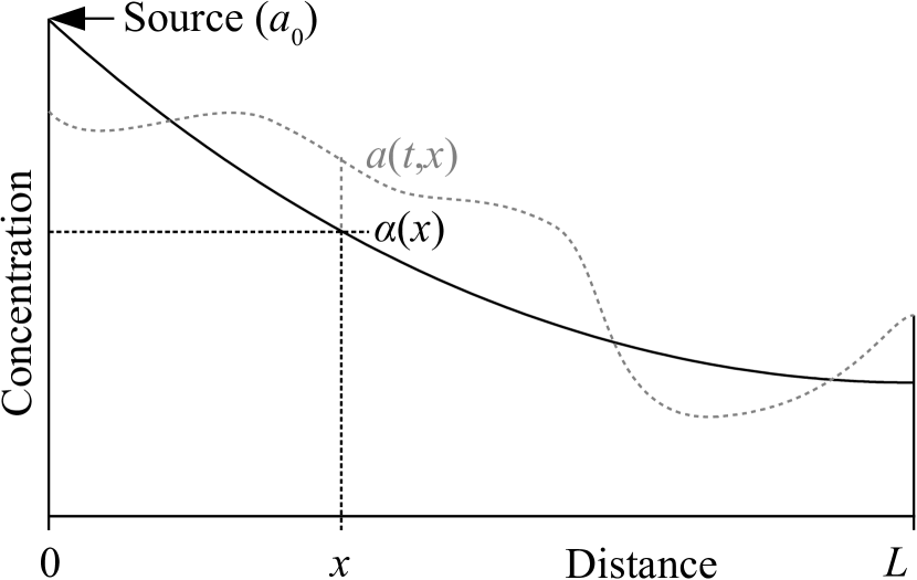
Figure 1: A morphogen produced at the left boundary propagates by diffusion into the rest of the one-dimensional system $\Lambda=[0,L]$. The morphogen’s steady-state concentration $\alpha(x)$ owing to a degradation reaction decreases monotonically towards the impenetrable right boundary. Each position coordinate $x\in\Lambda$ corresponds to a unique value of the positional-information curve $\alpha(x)$. The instantaneous concentration of the morphogen $a(t,x)$, however, is subject to spontaneous fluctuations on a mesoscopic scale.

Quantitative characterization of PI noise is an important problem in biophysics Gregor et al. (2007a, b); Bollenbach et al. (2008); Dubuis et al. (2013); Tkačik et al. (2015); Buceta (2017). Because many key processes in development occur on micrometer scales, the underlying chemical reactions and diffusive flows are subject to spontaneous variations. These fluctuations disrupt the local concentration of the morphogen and reduce the amount of information that a RD system contains Gregor et al. (2007a); Dubuis et al. (2013); Tkačik et al. (2015). A relevant question is then: how reliably can PI be encoded and read out in the presence of noise?

Most studies concentrate on the problem of decoding PI. For example, one can estimate the efficiency with which a cell measures a morphogen’s concentration Berg and Purcell (1977); Gregor et al. (2007a). The concentration can also be measured Gregor et al. (2007a, b); the experimental precision then provides an upper bound for the uncertainty of PI. Our understanding of the readout problem is incomplete, however, for one should also take into account how much information a noisy RD system actually contains.

The physical theory of fluctuations opens an avenue to the problem of encoding PI. At the mesoscopic scale, the dynamics of a reaction-diffusion system can be described by a stochastic partial differential equation derived from simplified microscopic mechanics van Kampen (2007, 1976); Gardiner (2004). The noise level in this model is completely determined by the macroscopic parameters of the system, such as the diffusion and reaction constants. The magnitude of fluctuations in the morphogen’s concentration should then in theory be calculable. This approach promises clearer results on the precision of PI than the analysis of empirical data.

As shown in Sec. II, the Van Kampen equation leads to a solution of infinite variance and therefore also of infinite standard deviation. Because both of these statistics measure the magnitude of fluctuations, one may regard this result as futile and seek a more realistic model. The existing alternatives [Chapter2in][]GOjalvaSancho; [Chapter8in][]Kotelenez; [Chapter1in][]Holder; [Sec.1.2.5in][]Lototsky either part ways with the Van Kampen equation or require an additional, ad hoc layer of theory. Both approaches, however, rely on new phenomenological constants such as the amplitude or correlation length of microscopic noise. Although these parameters control and regulate the fluctuation’s magnitude, they can be inferred neither from the meso- or macroscopic dynamics nor from the ensuing theory itself. Because one can only fit the new parameters to observations, these models are purely descriptive. This lack of predictive power is one reason why the theoretical avenue to the problem of encoding PI has received little attention.

In contradistinction to the theoretical approaches mentioned above, we estimate the fluctuations in a PI problem by solving the Van Kampen equation without modifications. A plausible level of noise is obtained if the resultant morphogen concentration is integrated in space over a subscale of the RD system. This procedure is consistent with classical fluid dynamics, in which macroscopic fields are commonly understood as coarse-grained representations of microscopic systems [Sec.I.1in][]LandauLifshitz6; [Sec.1.2; p.6in][]KardarII.

Multiscale models of computational physics, which combine the methods of finite elements and molecular dynamics Mortazavi et al. (2013); Kojic et al. (2014), make the coarse-graining procedure even more explicit. The macroscopic properties of a molecular-dynamics system are calculated as spatial averages by means of a microscopic connection (Evans and Morriss, 2007, Sec. 3 and 6). The exact procedure amounts to integration of molecular degrees of freedom over volume, which is suggestive of the coarse-graining subscale. The finite-element method then offers techniques to solve the dynamical equations of macroscopic fields. Note that, as the volume of a molecular-dynamics system decreases, the uncertainty of spatial averages diverges, exactly as in the Van Kampen theory.

A coarse-graining subscale arises quite naturally in developmental biology: morphogenetic features are not point-like, but have a finite mesoscopic extent in space. Moreover, developmental decisions are often delegated to whole cells or to large organelles such as cellular nuclei Gregor et al. (2007a); Buceta (2017). In the RD problems of morphogenesis and PI, one should therefore reckon with the total amount of the substance and its fluctuations over the scale of the target biological structure, rather than with the concentration field at isolated points.

In the next section we briefly describe the Van Kampen equation and the coarse-graining of its solution for a simple RD system. The implications of this theory and some numerical results are then discussed in Sec. III. Additional mathematical details are provided in the Appendices. In particular, Appendices C and D concern two classes of the finite-element method used to simulate numerically the dynamics of the coarse-grained stochastic fields.

II Theory

Because RD problems in general may not yield to analytical techniques, we use as a case study our earlier example of a simple one-dimensional system (Fig. 1). The associated theory can be treated by a variety of methods. Purely numerical techniques then can be compared with a more accurate analytical approach. This example is not entirely abstract, for it provides a model of the actual mechanism of PI encoding in Drosophila embryos Gregor et al. (2007a); Grimm et al. (2010).

In one dimension the number density of a morphogen $a(t,x)$, which depends on time $t$ and position $x$, obeys the Van Kampen dynamic equation van Kampen (2007, 1976); Gardiner (2004)

$$(\partial_{t}+k-D\partial_{x}^{2})a(t,x)=f(t,x),$$ (1)

in which the degradation rate $k$ and the diffusivity $D$ are positive constants, whereas $f(t,x)$ represents microscopic noise. Appendix A offers a short justification of the Van Kampen equation.

The left-hand side of Eq. (1) expresses the difference between the local change of concentration $\partial_{t}a(t,x)$ and the classical nonequilibrium forces of mass action and Fick’s diffusion. In small systems the residual force $f(t,x)$ does not vanish, but varies spontaneously because of microscopic events: this is the origin of microscopic noise. To be consistent with classical fluid dynamics, the steady-state ensemble averages of $f(t,x)$ and $a(t,x)$ must yield

$$\langle f(t,x)\rangle=0,\quad\langle a(t,x)\rangle=\alpha(x),$$ (2)

in which $\alpha(x)$—the PI curve—is the time-independent solution of the macroscopic RD problem [Fig. 1; Eq. (20) in Appendix A].

A convenient model of the morphogen’s source is a fixed-value condition imposed at the left end of the interval $\Lambda=[0,L]$. In the macroscopic RD problem, this constraint is supplemented quite naturally by a reflective right boundary, leading to the expression (20) for the concentration curve $\alpha(x)$. Nonetheless, in Appendices A and E we employ a different choice of the right boundary condition for the stochastic equation (1):

$$a(t,x)\Big{|}_{x=0}=a_{0}=\alpha(0),\quad a(t,x)\Big{|}_{x=L}=\alpha(L),$$ (3)

with $a_{0}$ representing a source of constant strength. By virtue of Eq. (2), the fixed-value boundary condition remains macroscopically consistent with the reflective boundary for the PI curve:

$$\partial_{x}\alpha(x)\Big{|}_{x=L}=0.$$ (4)

The problem of boundary conditions is addressed in Appendix E.

At the mesoscale and in the tradition of fluctuation theory, Van Kampen relates $f(t,x)$ to two stochastic terms, owing to the fluctuations of the mass-action law and the diffusive flow, respectively:

$$f(t,x)=\sqrt{k\alpha(x)}\partial_{x}\dot{W}_{1}(t,x)\\ +\partial_{x}[\sqrt{2D\alpha(x)}\partial_{x}\dot{W}_{2}(t,x)].$$ (5)

Here $\partial_{x}\dot{W}_{1}$ and $\partial_{x}\dot{W}_{2}$ are independent, spatially distributed, Gaussian white-noise variates of zero mean and unit strength (Appendix A). The overscript dots indicate the time derivatives. These noise sources are delta-correlated in both space and time:

$$\langle\partial_{x}\dot{W}_{1}\Big{|}_{t_{1},x_{1}}\partial_{x}\dot{W}_{2}\Big{|}_{t_{2},x_{2}}\rangle=0,$$ (6)

$$\langle\partial_{x}\dot{W}_{i}\Big{|}_{t_{1},x_{1}}\partial_{x}\dot{W}_{i}\Big{|}_{t_{2},x_{2}}\rangle=\delta(t_{1}-t_{2})\delta(x_{1}-x_{2}),$$ (7)

which hold for $i=1,2$, with $\delta(\cdot)$ being the Dirac delta function. Note in the above equations that spatially distributed white noise is singular in time and space: its variance diverges as a product of two delta functions, $\lim_{t\to 0}\delta(t)$ and $\lim_{x\to 0}\delta(x)$.

To avoid immaterial details, we focus on the steady-state solution of Eq. (1), $a(\infty,x)$. We denote the deviation of the morphogen’s concentration from the ensemble average value by $\Delta{a}(t,x)=a(t,x)-\alpha(x)$. Then Eq. (34) of Appendix B gives us

$$\Delta{a}(\infty,x)=\lim_{t\to\infty}\int_{0}^{t}dt^{\prime}\int_{\Lambda}dx^{\prime}g(t-t^{\prime},x|x^{\prime})f(t^{\prime},x^{\prime}).$$ (8)

Here $g(t-t^{\prime},x|x^{\prime})$ is the Green’s function that propagates disturbances of the number density in time and space, from an instant $t^{\prime}$ and position $x^{\prime}$ to any other $t$ and $x$.

The steady-state variance of the deviation $\Delta{a}(\infty,x)$, as can be formally calculated from Eq. (8), diverges [see also Eq. (35) in Appendix B]. To understand why this happens, apply the differential chain rule to the second term on the right-hand side of Eq. (5) and substitute it into Eq. (8); one then finds the following term in the expression for $\Delta{a}(\infty,x)$:

$$\lim_{t\to\infty}\int_{0}^{t}dt^{\prime}\int_{\Lambda}dx^{\prime}g(t-t^{\prime},x|x^{\prime})\sqrt{2D\alpha(x^{\prime})}\partial_{x^{\prime}}^{2}\dot{W}_{2}(t^{\prime},x^{\prime})\\ \sim\partial_{x}W_{2}(t,x).$$ (9)

Here the time integration removes the temporal singularity of $\partial_{x}^{2}\dot{W}_{2}$, but the spatial integral is canceled by one of the two derivative operators. The above term contains a spatial singularity of the order $\partial_{x}W_{2}(t,x)$ [Eq. (7)]. Therefore the variance of $\Delta{a}(\infty,x)$, expressed formally by Eq. (35), in effect diverges.

If one replaces the positional delta function $\delta(\cdot)$ in Eq. (7) by some bounded correlation kernel $C(\cdot)$ (Garcia-Ojalvo and Sancho, 1999, Sec. 2.1.2), the spatial singularity disappears from Eqs. (8) and (9). The cost of this approach is a significantly more complicated theory Stefanou (2009); Sepahvand et al. (2010); [Chapter2in][]Ghanem. First, spatial noise correlations that regularize the variance of $\Delta{a}(\infty,x)$ must be modeled explicitly. Second, a nontrivial kernel $C(\cdot)$ increases the mathematical difficulty of the problem. The spatial singularity of Eq. (9) can alternatively be removed by integrating it with respect to the coordinate $x$, the approach that we pursue here. An integration with respect to position occurs when we coarse-grain the number density $a(t,x)$ over a scale $\xi$ of the appropriate spatial dimension. Then, instead of the morphogen’s concentration at some point $x$, the quantity of interest becomes the total number of molecules in the $\xi$-neighborhood $\Xi(x)=(x-\xi/2,x+\xi/2)$ of that point. If we use the inverse scale $\xi$ as a normalization factor, we can equivalently consider a coarse-grained concentration field

$$a_{\xi}(x)=\int_{x-\xi/2}^{x+\xi/2}\frac{dx^{\prime}}{\xi}a(\infty,x^{\prime}).$$ (10)

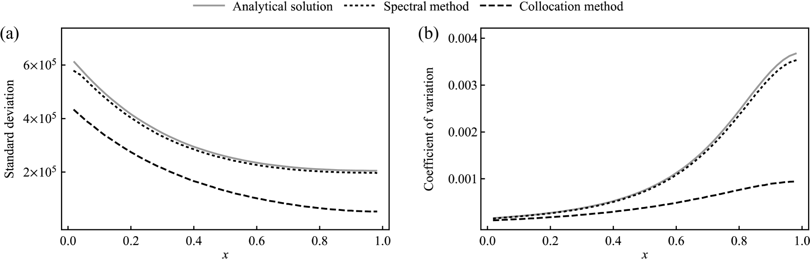
Figure 2: Uncertainty of the coarse-grained concentration $\alpha_{\xi}(x)$ as a function of position for the experimental data of Refs. Gregor et al. (2007a); Grimm et al. (2010). The values of the standard deviation in A and the coefficient of variation in B are calculated by three methods: i) analytical solution (Appendix B); ii) spectral finite-element simulations (Appendix C); iii) collocation finite-element method (Appendix D). The uncertainty of the PI curve does not exceed $0.4\,\%$ at any position.

The coarse-grained concentration of the morphogen undergoes fluctuations of finite magnitude. As a statistical measure of this magnitude one can take either the variance of $a_{\xi}$—the second cumulant $\kappa_{2}(a_{\xi})$—or the standard deviation $\operatorname{std}(a_{\xi})$. By using the properties of the Green’s and delta functions together with Eqs. (3)–(8), we find

$$\kappa_{2}[a_{\xi}(x)]=\iint_{\Xi(x)}\frac{dx_{1}dx_{2}}{\xi^{2}}\lim_{t\to\infty}\int_{0}^{t}dt^{\prime}\int_{\Lambda}dx^{\prime}\alpha(x^{\prime})\\ \times\Big{[}kg(t-t^{\prime},x_{1}|x^{\prime})g(t-t^{\prime},x_{2}|x^{\prime})\\ +2D\partial_{x^{\prime}}g(t-t^{\prime},x_{1}|x^{\prime})\partial_{x^{\prime}}g(t-t^{\prime},x_{2}|x^{\prime})\Big{]}.$$ (11)

A Fourier series expansion of the above expression, as well as of the coarse-grained steady-state concentration $\alpha_{\xi}(x)$, is derived in Appendix B [Eqs. (37) and (38)]. The number density $\alpha_{\xi}(x)$ differs from $\alpha(x)$ by a factor that is negligible for small scales $\xi$. Both these fields interchangeably represent a PI curve, for they convey nearly the same value everywhere in $\Lambda$.

A useful way to quantify the uncertainty of $a_{\xi}(x)$ is the coefficient of variation, $\operatorname{std}(a_{\xi})/\alpha_{\xi}$, which relates the level of fluctuations to the strength of the PI signal. Quite generally, however, both the mean value of the morphogen’s concentration and its variance are proportional to the parameter $a_{0}$ [Eq. (37) and (38), Appendix B]. Therefore the relative uncertainty is inversely proportional to $\sqrt{a_{0}}$:

$$\frac{\operatorname{std}[a_{\xi}(x)]}{\alpha_{\xi}(x)}=\frac{\sigma_{\xi}(x|\ell)}{\sqrt{a_{0}}},$$ (12)

in which $\sigma_{\xi}(x|\ell)$ depends only on the coordinate $x$ and the parameters $\xi$ and $\ell=\sqrt{D/k}L^{-1}$.

Fluctuations of physical quantities usually decay as the inverse square root of the number of molecules involved [Sec.I.2in][]LandauLifshitz5. This dependence is explicitly controlled by the parameter $a_{0}$ in Eq. (12). The source strength $a_{0}$ in the above expression should therefore be measured in one dimension as the number of molecules per unit length. If molar or mass-density units are used instead, Eq. (12) does not render the coefficient of variation correctly.

Equation (12) defines $\sigma_{\xi}(x|\ell)$, which we call a variation profile. Given the values of $\xi$ and $\ell$, this relation can be evaluated numerically as a function of position by use of Eqs. (37) and (38). For a source of any given strength $a_{0}$, the coefficient of variation—a rescaled variation profile—can then be calculated easily from Eq. (12).

Finally, the constant $\ell>0$ is the correlation parameter of $a_{\xi}(x)$ [Appendix B, Eq. (40)]. The fluctuations of the morphogen’s concentration at two points separated by distances greater than $\ell L=\sqrt{D/k}$ are nearly independent, whereas the decay of the time correlations is controlled by $(k\ell^{2})^{-1}=L^{2}/D$ (Appendix B). The constants $k$ and $L$ determine the scale of the system; they can serve as units of time and length.

III Numerical results

As an application of the Van Kampen theory, we estimate the level of fluctuations for the concentration of the morphogen bicoid in a Drosophila embryo Gregor et al. (2007a); Grimm et al. (2010). The results of our calculations are reported in a system of units reduced by the length constant $L$ and the time constant $k^{-1}$. The values of the physical parameters are adopted from experimental data Gregor et al. (2007a); Grimm et al. (2010): $L=0.5$ mm, $\lambda=0.1$ mm, $a_{0}=55$ nM (1 nM corresponds to 0.6 molecules/$\mu$m³). Converted to reduced units, the source strength and the correlation length are respectively $a_{0}=4.125\times 10^{9}$ and $\ell=0.2$. The concentration of bicoid is presumably read out by densely distributed cellular nuclei, whose spatial separation sets a plausible coarse-grain scale of $\xi=0.02$.

Figure 2 (a) illustrates a typical dependence of the standard deviation $\operatorname{std}(a_{\xi})$ on the position $x$, calculated for the coarse-grained PI curve. This is a convex curve that is defined over the interval $[\xi/2,L-\xi/2]$ and decreases monotonically from its maximum at $x=\xi/2$. For large correlation lengths $\lambda=\ell L$, the variance of the coarse-grained morphogen concentration depends almost linearly on $x$ and flattens when $\lambda\to\infty$ and $k\to 0$. In the latter case, which represents pure diffusion without degradation, the fluctuations of $\alpha(x)$ are maximal for any given values of $a_{0}>0$ and $\xi>0$. On the other hand, when the rate constant $k$ becomes infinitely large, the problem degenerates and fluctuations vanish.

Of the two numerical integration schemes discussed in this paper, the collocation method (Appendix D) is less accurate than the spectral finite-element algorithm (Appendix C). The latter approach compares favorably with the analytical solution [Eq. (37) in Appendix B]. Both integration algorithms nonetheless reproduce correctly the average concentration and the overall shape of the variation profile.

The relative uncertainty of the PI curve in our numerical example does not exceed $0.4\,\%$ at any position [Fig. 2 (b)]. Because $\alpha_{\xi}$ decreases with $x$ faster than its standard deviation, the coefficient of variation increases towards the right boundary. The relative uncertainty nevertheless remains within the order of $0.2\,\%$ in most of the system. Even an error of three standard deviations still yields a coefficient of variation within the order of $1\,\%$. The precision of the PI readout might therefore be limited mainly by the efficiency of the morphogen’s receptors.

Because the modeled system is half a milimeter in length Gregor et al. (2007a), the small uncertainty of the PI curve in our example comes as no surprise. Given a target precision of $10\,\%$ Gregor et al. (2007a), the concentration of bicoid can be measured in a period of time that is very short in comparison to the correlation scale $(k\ell)^{-1}$. This result validates the Van Kampen theory for conditions approaching the macroscopic limit. However, in developmental processes on a scale of tens of micrometers Jacobo and Hudspeth (2014)—the dimension relevant to the specification of intracellular structures—fluctuations can challenge the efficiency of morphogen receptors. Additional mechanisms, such as biochemical feedback loops Dublanche et al. (2006), might then be required to reduce noise in the system.

IV Conclusion

The Van Kampen theory provides a promising means of estimating the fluctuation level in RD problems and more generally in systems of mesoscopic physical fields. The approach is conceptually simple and has a relatively small computational cost. Although in this paper we consider only the steady-state solution of a RD problem, transients can be taken into account as well [Eq. (33) in Appendix B]. Moreover, the Van Kampen theory can be integrated readily into multiscale computational models.

To simulate the Van Kampen equation, we formulated and tested two numerical techniques. The results of spectral finite-element simulations (Appendix C) were quite accurate and superior to those of the collocation method (Appendix D).

As a case study we chose a relatively large, 500 $\mu$m-long system for its simple geometry and the availability of experimental data. Because the length scale approaches macroscopic conditions, fluctuations of the PI curve in our simple example are very small. In many other instances of the PI problem, however, the system’s size can be 10 $\mu$m or even less. At such scales, the fluctuations of the PI curve can impose operational time and space constraints on the detectors of morphogen concentration. Estimation of the noise level might provide insight into the mechanisms of encoding and readout of PI. For example, the concentration’s uncertainty might help in identifying a morphogen among the candidate substances that occur in a system.

In a study focused on a specific RD problem, there are more details that could be included in a Van Kampen equation: fluctuations of the source strength, boundary effects, and the dimensionality of the system. Incorporation of these factors should improve the accuracy of a theoretical model (Appendices B and E).

Appendix A Van Kampen reaction-diffusion equation

The Van Kampen RD equation (1) extends the Langevin model of fluctuations for simple time-dependent physical quantities to spatially distributed fields van Kampen (2007, 1976); Gardiner (2004). Consider first the classical RD dynamics for the number density $a(t,x)$ of some morphogen over the linear domain $x\in\Lambda$:

$$\partial_{t}a(t,x)=-ka(t,x)+D\partial_{x}^{2}a(t,x),$$ (13)

in which the degradation rate $k$ and the diffusivity $D$ are positive constants. The first term on the right-hand side of Eq. (13) states the mass-action law for the chemical degradation of the morphogen. The second term represents the divergence of the Fick’s diffusion flow

$$J(t,x)=-D\partial_{x}a\,\Rightarrow\,-\partial_{x}J(t,x)=D\partial_{x}^{2}a,$$ (14)

which describes the balance of incoming and outgoing currents of matter $J(t,x)$.

Both macroscopic laws—mass action and Fick’s diffusion—emerge as statistical averages of the microscopic dynamics van Kampen (2007, 1976) over a steady-state ensemble. Ergodicity of a system is commonly assumed as well. At mesoscopic scales, however, we must allow fluctuations by replacing the following terms in Eqs. (13) and (14):

$$ka(t,x) \to ka(t,x)-\chi(t,x),$$

$$J(t,x) \to-D\partial_{x}a(t,x)-j(t,x),$$ (15)

in which $\chi(t,x)$ and $j(t,x)$ are the deviations from the classical macroscopic laws of reaction and diffusion, respectively. Due to the spontaneous variations given by Eqs. (A), the local change of concentration $\partial_{t}a(t,x)$ does not exactly match the fluctuating force on the right-hand side of Eq. (13). The residual is

$$(\partial_{t}+k-D\partial_{x}^{2})a(t,x)=\chi(t,x)+\partial_{x}j(t,x).$$ (16)

The spontaneous behavior of the fluctuating force on the right-hand side of this equation appears practically random and is therefore modeled as a stochastic, spatially distributed process.

In the Langevin approach, the macroscopic properties of a steady-state dynamics correspond to the ensemble averages, here denoted by angle brackets, of mesoscopic variables. In particular, Eq. (13) requires $\langle\chi(t,x)\rangle=0$ and $\langle\partial_{x}j(t,x)\rangle=~{}0$. Hence the ensemble average of Eq. (16) yields

$$k\langle a(t,x)\rangle-D\partial_{x}^{2}\langle a(t,x)\rangle=0$$ (17)

for $\langle\partial_{t}a(t,x)\rangle=0$ by the definition of a steady state.

For a nontrivial solution $\langle a(t,x)\rangle\neq 0$ to exist, we model a source of the chemical agent by a nonhomogeneous Dirichlet boundary condition, which fixes the value of $\langle a(t,x)\rangle$ at $x=0$:

$$\langle a(t,0)\rangle=a_{0}.$$ (18)

A natural choice of the other boundary at $x=L$ is the homogeneous Neumann condition, which reflects the diffusive flow $\langle J(t,x)\rangle$ [Eq. (A)]:

$$\langle\partial_{x}a(t,L)\rangle=0.$$ (19)

Subject to the above constraints, Eq. (17) is easy to solve (Edwards and Penney, 2008, Chapter 2). We thus obtain the macroscopic time-independent PI curve plotted in Fig. 1,

$$\alpha(x)=\langle a(t,x)\rangle=a_{0}\frac{\cosh[(L-x)/\lambda]}{\cosh(L/\lambda)},$$ (20)

in which $\lambda=\sqrt{D/k}$.

For Langevin dynamics (19) we reduce the homogeneous Neumann condition at the right end to a consistent nonhomogeneous Dirichlet boundary:

$$\langle a(t,L)\rangle=\alpha(L).$$ (21)

As discussed in Appendix E, both Dirichlet conditions (18) and (21) neglect fluctuation effects at the boundaries of the RD system. These effects can be included by imposing the reflective Neumann conditions on both ends of $\Lambda$. These details, which are not strictly necessary for a simple demonstration of the Van Kampen theory, are spared for Appendix E.

The Langevin model is complete once the statistical properties for the right-hand side of Eq. (16) have been specified. Van Kampen derives them by reducing the microscopic RD dynamics to a random walk, a traditional argument of statistical mechanics [ChapterIin][]Chandrasekhar; *Piasecki. A continuous limit of this simplified model gives

$$\langle\chi(t,x)\chi(t^{\prime},x^{\prime})\rangle=k\alpha(x)\delta(t-t^{\prime})\delta(x-x^{\prime}),$$ (22)

$$\langle j(t,x)j(t^{\prime},x^{\prime})\rangle=2D\alpha(x)\delta(t-t^{\prime})\delta(x-x^{\prime}),$$ (23)

which hold for any instants of time $t,t^{\prime}$, and positions $x,x^{\prime}$ van Kampen (2007, 1976). The theory behind the above equations relies on the following assumptions: $\chi$ and $j$ are independent ($\langle\chi(t,x)j(t^{\prime},x^{\prime})\rangle\equiv 0$); an infinitesimal interval $dx$ contains a large number of molecules $\alpha(x)dx$; and all correlations at distances of order $dx$ are negligible. Then infinitesimal processes $\chi(t,x)$ and $j(t,x)$ are approximately Gaussian by virtue of the central limit theorem (Kardar, 2007b, Sec. 2.5).

The Van Kampen model leads directly to the concept of a spatially distributed Gaussian white noise $\partial_{x}\dot{W}(t,x)$ with a zero mean and a constant strength $\beta$. The defining property of $\partial_{x}\dot{W}$ is that its integral over a time interval $t$ and a line segment $\Xi(x)=(x-\xi/2,x+\xi/2)$,

$$W(t,x|\xi)=\int_{0}^{t}dt^{\prime}\int_{\Xi(x)}dx^{\prime}\partial_{x^{\prime}}\dot{W}(t^{\prime},x^{\prime}),$$ (24)

is a Gaussian random process of zero mean ($\langle W\rangle=0$) and variance

$$\langle W(t,x|\xi)^{2}\rangle=\beta\xi t.$$ (25)

All properties of the stochastic processes $\chi(t,x)$ and $j(t,x)$ are then encompassed by

$$\chi(t,x)=\sqrt{k\alpha(x)}\partial_{x}\dot{W}_{1}(t,x),$$ (26)

$$j(t,x)=\sqrt{2D\alpha(x)}\partial_{x}\dot{W}_{2}(t,x),$$ (27)

in which $\partial_{x}\dot{W}_{1}$ and $\partial_{x}\dot{W}_{2}$ are two independent, spatially distributed, Gaussian white-noise terms of unit strength $\beta=1$ [Eqs. (6) and (7)]. Note that $j(t,x)$ is a vector quantity, which in one dimension has a single component $\partial_{x}\dot{W}_{2}(t,x)$.

Appendix B Green’s function method

Supplemented with an initial value $a(0,x)$ and the boundary conditions (3), Eqs. (16)–(27) lead to Eq. (1):

$$(\partial_{t}+k-D\partial_{x}^{2})a(t,x)=f(t,x).$$

This stochastic partial differential equation is linear, as is its left-hand-side operator $\mathcal{L}=(\partial_{t}+k-D\partial_{x}^{2})$, and inhomogeneous, in that $f(t,x)$ enters the expression additively.

A general solution of Eq. (1) is most conveniently expressed with the help of the Green’s function (Arfken et al., 2013, Chapter 10) $g(t-t^{\prime},x|x^{\prime})$, which we find from the following equations:

$$\mathcal{L}g(t-t^{\prime},x|x^{\prime})=\delta(t-t^{\prime})\delta(x-x^{\prime}),$$ (28)

$$g(t,0)=g(t,L)=0.$$ (29)

In a finite domain $\Lambda$ the Green’s function can be expanded as a series [Secs.2.4and4.2in][]Duffy2001; *[Secs.3.4and5.2in][]Duffy2015. For the problem at hand we use a discrete expansion ($n=1,2...$) in the orthonormal Fourier basis

$$\phi_{n}(x)=\sqrt{2/L}\sin(n\pi x/L),$$ (30)

which is complete under the boundary conditions (29). One then finds

$$g(t-t^{\prime},x|x^{\prime})=\sum_{n=1}^{\infty}g_{n}(t-t^{\prime})\phi_{n}(x^{\prime})\phi_{n}(x),$$ (31)

$$g_{n}(t)=H(t)\exp\left\{-t\left[k+D\frac{n^{2}\pi^{2}}{L^{2}}\right]\right\},$$ (32)

in which $H(\cdot)$ stands for the Heaviside step function.

With the boundary conditions (3) and (29), the general solution of (1) takes the form

$$a(t,x)=\alpha(x)+\int_{\Lambda}dx^{\prime}g(t,x|x^{\prime})[a(0,x^{\prime})-\alpha(x^{\prime})]\\ +\int_{0}^{t}dt^{\prime}\int_{\Lambda}dx^{\prime}g(t-t^{\prime},x|x^{\prime})f(t^{\prime},x^{\prime}),$$ (33)

in which the second term on the right-hand side vanishes as $\lim_{t\to\infty}g(t,x|x^{\prime})=0$. If one is concerned merely with the steady-state behavior of Eq. (1), the transient solutions can be eliminated from Eq. (33) by taking the limit of infinite $t$:

$$a(\infty,x)=\alpha(x)\\ +\lim_{t\to\infty}\int_{0}^{t}dt^{\prime}\int_{\Lambda}dx^{\prime}g(t-t^{\prime},x|x^{\prime})f(t^{\prime},x^{\prime}).$$ (34)

Consider the statistical properties of the steady-state solution $a(\infty,x)$. Because $f(t,x)$ given by Eqs. (5) is a linear superposition of zero-mean, Gaussian white-noise terms, the ensemble average of Eq. (34) is consistent with the macroscopic dynamics (13):

$$\langle a(\infty,x)\rangle=\alpha(x).$$

The second cumulant $\kappa_{2}[a(\infty,x)]$ of $a(\infty,x)$ can be obtained from Eqs. (3)–(8), and (29):

$$\kappa_{2}[a(\infty,x)]=\kappa_{2}[\Delta{a}(\infty,x)]=\langle a(\infty,x)^{2}-\alpha(x)^{2}\rangle\\ =k\lim_{t\to\infty}\int_{0}^{t}dt^{\prime}\int_{\Lambda}dx^{\prime}\alpha(x^{\prime})[g(t-t^{\prime},x|x^{\prime})]^{2}\\ +2D\lim_{t\to\infty}\int_{0}^{t}dt^{\prime}\int_{\Lambda}dx^{\prime}\alpha(x^{\prime})[\partial_{x^{\prime}}g(t-t^{\prime},x|x^{\prime})]^{2}.$$ (35)

Higher-order cumulants of the steady-state solution vanish due to the Gaussian nature of $f(t,x)$ and hence of $\alpha(\infty,x)$ as well.

As explained in Sec. II, the formal expression (35) diverges. Therefore, to estimate the magnitude of fluctuations in the morphogen’s concentration, we calculate the variance of the coarse-grained number density $a_{\xi}(\infty,x)$ from Eq. (11). This computation can be carried out through a series expansion of the Green’s function, $g(t-t^{\prime},x|x^{\prime})$, truncated at $N$th term. Let us introduce the following formulas:

$$\Phi_{n}(x)=\int_{\Xi(x)}\frac{dx^{\prime}}{\xi}\phi_{n}(x^{\prime})=\frac{2L}{n\pi\xi}\sin\left(\frac{n\pi\xi}{2L}\right)\phi_{n}(x);$$

$$\Omega_{mn}=\frac{4\pi^{2}\ell^{3}mn\tanh[\ell^{-1}]}{[1+\pi^{2}\ell^{2}(m-n)^{2}][1+\pi^{2}\ell^{2}(m+n)^{2}]},$$ (36)

in which $\ell=\sqrt{D/k}L^{-1}$. Then, by substituting Eqs. (20), (31), and (32) into (11) and completing the integrals, we obtain

$$\kappa_{2}[a_{\xi}(x)]=a_{0}\sum_{mn}\Omega_{mn}\Phi_{m}(x)\Phi_{n}(x),$$ (37)

in which the summation runs over all positive integers $m$ and $n$ up to $N$ ($m,n=1..N$). Note that the mean value of the coarse-grained field $a_{\xi}(x)$ is

$$\langle a_{\xi}(x)\rangle=\frac{2\lambda}{\xi}\sinh\left(\frac{\xi}{2\lambda}\right)\alpha(x)\underset{\xi\to 0}{\to}\alpha(x).$$ (38)

We can similarly obtain the autocorrelation function $\kappa_{2}[a_{\xi}(0,x_{1}),a_{\xi}(t,x_{2})]$ for the time-dependent concentration

$$a_{\xi}(t,x)=\int_{\Xi(x)}dx^{\prime}a(t,x^{\prime})=\alpha_{\xi}(x)+\Delta{a}_{\xi}(t,x).$$ (39)

In linear systems the decay of the temporal and spatial autocorrelations is encompassed by the Green’s function (Chandler, 1987, Sec. 8.6):

$$\kappa_{2}[a_{\xi}(0,x_{1}),a_{\xi}(t,x_{2})]=\langle\Delta{a}_{\xi}(0,x_{1})\Delta{a}_{\xi}(t,x_{2})\rangle=\\ \int_{\Lambda}dx^{\prime}g(t,x_{2}|x^{\prime})\langle\Delta{a}_{\xi}(0,x_{1})\Delta{a}(0,x^{\prime})\rangle=\\ a_{0}\sum_{mn}\Omega_{mn}\Phi_{m}(x_{1})\Phi_{n}(x_{2})\exp[-kt(1+\pi^{2}\ell^{2}m^{2})],$$ (40)

in which only the transient term of Eq. (33) makes a non-zero contribution Belousov and Cohen (2016). From Eqs. (31), (32), (B), and (40) it follows that, in reduced units (Sec. III), the time and space correlations are controlled respectively by the parameters $(k\ell)^{2}=D/L^{2}$ and $\lambda=\ell L=\sqrt{D/k}$ through the diffusion constant $D$.

In computations the series expansion (37) and (40) should be truncated at an order $N\geq\lceil{2L/\xi}\rceil$. This optimal value is suggested by the following argument. Suppose that $2L/\xi$ is an integer. The Fourier mode $\phi_{n+N}(\cdot)$ is then an alias of $\phi_{n}(\cdot)$, because $\phi_{n+N}(x)=\phi_{n}(x)$ whenever $x$ is an integer multiple of $\xi$. In Eq. (37) we passed from the basis set $\phi_{n}(\cdot)$ to the coarse-grained functions $\Phi_{n}(\cdot)$ by integrating over a spatial scale $\xi$ [Eq. (B)]. This procedure allows us to disregard aliasing modes with $n>N$. Indeed, spatial features smaller than the scale $\xi$ should be smoothed by the coarse-graining integration. The regions near the ends of the domain $\Lambda$ ($x\approx\xi/2,L-\xi/2$) are exceptions that may require more terms to reduce ringing artifacts.

Appendix C Spectral method

Modal analysis similar to that of Appendix B leads to a simple method of spectral finite elements Trefethen (2000); van de Vosse and Minev (1996); Boyd (2000) for Eq. (1). Subject to the boundary conditions (3), the number density $a(t,x)$ has a series representation in terms of the basis functions given by Eq. (30):

$$a(t,x)=\alpha(x)+\sum_{m=1}^{\infty}a_{m}(t)\phi_{m}(x),$$ (41)

in which the time-dependent coefficients $a_{m}(t)$ must vanish on average to satisfy Eq. (2): $\langle a_{m}(t)\rangle=0$.

Spatially distributed white noise $\partial_{x}\dot{W}_{i}$ ($i=1,2$) likewise has a representation

$$\partial_{x}\dot{W}_{i}(t,x)=\sum_{n=1}^{\infty}\dot{w}_{in}(t)\phi_{n}(x),$$ (42)

in which each time-dependent coefficient $\dot{w}_{in}(t)$ is a simple, independent Gaussian white noise. Equations (6), (7), (24), and (25) readily follow from Eq. (42). In higher dimensions there are additional vector components like $\partial_{x}\dot{W}_{2}$ (Appendix B) that are independent in an orthogonal reference frame and therefore can be expanded separately in series (42). In nonorthogonal coordinate systems one must also account for correlations due to the overlap of basis vectors.

Equations (41) and (42), truncated at some $m$ and $n$, provide the finite-element representations of $a(t,x)$ and the white-noise terms. Their substitution into (1) and a few simple manipulations eventually lead to a system of ordinary differential equations for the coefficients $a_{m}(t)$:

$$\dot{a}_{m}(t)=-k(1+\pi^{2}\ell^{2}m^{2})a_{m}(t)+f_{m}(t),$$ (43)

in which $\ell=\sqrt{D/k}L^{-1}$, and

$$f_{m}(t)=\sum_{n}\left[F_{1mn}\dot{w}_{1n}(t)+F_{2mn}\dot{w}_{2n}(t)\right],$$ (44)

$$F_{1mn}=\int_{\Lambda}dx\sqrt{k\alpha(x)}\phi_{m}(x)\phi_{n}(x),$$ (45)

$$F_{2mn}=-\int_{\Lambda}dx\sqrt{2D\alpha(x)}\partial_{x}\phi_{m}(x)\phi_{n}(x).$$ (46)

From Eq. (43) we see that stochastic forces $f_{m}(t)$ randomly perturb the modal coefficients $a_{m}(t)$. When explicit analytical expressions are not available for the spatial integrals in Eqs. (45) and (46), a discrete Fourier transform can be used instead as an approximation. This approach should then be termed a pseudospectral finite-element method.

For a general RD system, the derivation of equations analogous to (43) is quite straightforward. Because the problem studied in this paper is relatively simple, we can obtain each coefficient $a_{m}(t)$ explicitly (Appendix B). Because numerical methods are more widely applicable than analytical ones, however, we develop below a pseudospectral finite-element scheme to solve the system of equations (43).

The system of equations (43) can be numerically integrated in time by various methods, such as the Crank-Nicolson algorithm discussed in the next section of the Appendix. We can also use a second-order stochastic operator-splitting technique (Belousov et al., 2017, Appendix C):

$$a_{m}(t+\Delta{t})= \exp[-(1+\pi^{2}\ell^{2}m^{2})k\Delta{t}]a_{m}(t)$$

$$+ \exp\left[-(1+\pi^{2}\ell^{2}m^{2})\frac{k\Delta{t}}{2}\right]F_{m}(\Delta{t});$$

$$F_{m}(\Delta{t})= \int_{0}^{\Delta{t}}dt\,f_{m}(t)$$

$$= \sqrt{\Delta{t}}\sum_{n}[F_{1mn}w_{1n}+F_{2mn}w_{2n}],$$ (47)

in which $w_{1n}$ and $w_{2n}$ are independent Gaussian random variables of zero mean and unit variance, whereas $\Delta{t}$ is an integration time step.

By coarse-graining Eq. (41), one easily finds a finite-element representation of $\Delta{a}_{\xi}(x)=a_{\xi}(x)-\alpha_{\xi}(x)$ in the notation of Eq. (B):

$$\Delta{a}_{\xi}(x)=\sum_{m}a_{m}\Phi_{m}(x),$$ (48)

in which the coefficients $a_{m}$ are correlated Gaussian variables. Their covariance matrix

$$K_{mn}=\langle a_{m}a_{n}\rangle$$

can be sampled in a numerical simulation of Eq. (C). The variance of $\Delta{a}_{\xi}(x)$ is then equal to

$$\kappa_{2}[\Delta{a}_{\xi}(x)]=\sum_{mn}K_{mn}\Phi_{m}(x)\Phi_{n}(x).$$ (49)

By comparing the above equation with (37), we see that $K_{mn}=a_{0}\Omega_{mn}$.

The above results show that the modal coefficients $a_{m}(t)$ are correlated Gaussian random variables of finite mean and variance. However, there are so many of them in the representation of $a(\infty,x)$ that its variance given by Eq. (35) diverges unless the coarse-grained basis functions $\Phi_{m}(x)$ are used as in (37). Thanks to the nonsingular nature of the modal coefficients, a computer simulation of Eq. (C) is feasible.

The series expansions (41) and (42) need not have the same number of modes. The argument of Appendix B for Eq. (37) sets the optimum for $m=1,2,..N_{m}$, in which $N_{m}=\lceil{2L/\xi}\rceil$. The accuracy of simulations can be improved indefinitely by taking progressively more terms in Eq. (42), $N_{n}\geq N_{m}$. In Sec. III we report our results for $N_{n}=4N_{m}$ and $\Delta{t}=10^{-3}$.

Appendix D Collocation method

The Fourier components $a_{m}(t)$ of the morphogen’s concentration are Gaussian random variables of finite variance (Appendix C). This vector representation of the field $a(t,x)$ can be projected onto another basis set. Then, in principle, it should be possible to simulate numerically the dynamics of the new components.

In this section we use a piecewise-linear interpolation (Trefethen, 2000, Chapter 1), as a basis set for the finite-volume method, a widely used collocation finite-element scheme (Mattiussi, 1997; Versteeg and Malalasekera, 2007, Chapter 4). Consider a uniform grid $x_{i}=i\Delta{x},\,i=0,1,\dots M+1$ on the domain $\Lambda$ (Fig. 3). We center control elements of size $\Delta{x}$ at the nodes $x_{i},\,i=1,2,\dots M$. The morphogen’s concentration is then interpolated by

$$a(t,x) \approx \sum_{i=0}^{M+1}A_{i}(t)\eta_{i}(x),$$ (50)

$$\eta_{i}(x) = \begin{cases}\frac{\Delta{x}-x_{i}+x}{\Delta{x}},\;\text{if }x_{i-1}\leq x\leq x_{i}\\ \frac{\Delta{x}+x_{i}-x}{\Delta{x}},\;\text{if }x_{i}\leq x\leq x_{i+1}\\ \end{cases},$$ (51)

which coincides with $a(t,x)$ at the centers of the control elements $A_{i}(t)=a(t,x_{i})$. To comply with the boundary conditions (3), we fix $A_{0}=a_{0}$ and $A_{M+1}=\alpha(L)$. Thus the above interpolation is completely specified by $M$ time-dependent components $A_{i}(t),\,i=1..M$.

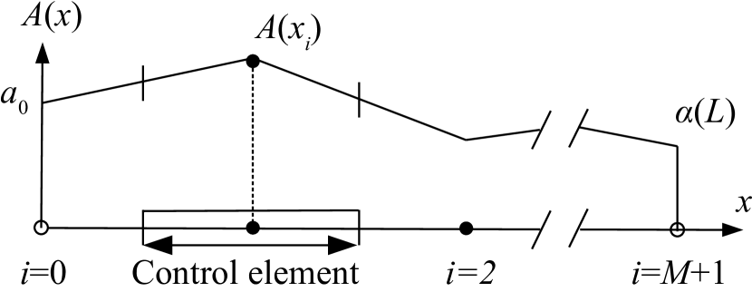
Figure 3: A piecewise-linear interpolant $A(x)$ on a grid $x_{i},\,i=0..M+1$. We use the boundary conditions (3) to fix the values $A(x_{0})=a_{0}$ and $A(x_{M+1})=\alpha(L)$ at the nodes $i=0$ and $i=M+1$ ($\circ$), respectively. The control elements are centered on the nodes $i=1..M$ ($\bullet$). This collocation scheme reserves small intervals near the boundaries of the domain for a convenient implementation of the coarse-graining procedure.

A standard procedure of the finite-volume method would be to integrate Eq. (1) over each $i$th control element $X_{i}=[x_{i}-\Delta{x}/2,x_{i}+\Delta{x}/2]$. In addition to this, we must apply coarse graining over the scale $\xi\geq\Delta{x}$ in order to remove the spatial singularity of the stochastic noise (Sec. II). It is convenient to partition the domain $\Lambda$ so that $\xi$ is an integer multiple of $\Delta{x}$: $\xi=P\Delta{x}$. We construct an integral operator

$$\mathcal{I}_{Pi}=P^{-1}\sum_{j=0}^{P-1}\mathcal{I}_{i+j}=P^{-1}\sum_{j=0}^{P-1}\iint_{X_{i+j}}\frac{dx^{2}}{\Delta{x}}.$$ (52)

In the above expression it suffices to consider only $P=1$ with a single term $\mathcal{I}_{i}$ that can be used to evaluate Eq. (52) for an arbitrary $P$. Applied to $a(t,x)$, the operator $\mathcal{I}_{i}$ gives a spatial integral of the coarse-grained concentration:

$$\mathcal{I}_{i}a(t,x)=\int_{X_{i}}dx_{1}\int_{x_{1}-\Delta{x}/2}^{x_{1}+\Delta{x}/2}\frac{dx_{2}}{\Delta{x}}\,a(t,x_{2})\\ =\int_{X_{i}}dx_{1}\,a_{\xi}(t,x_{1})\Big{|}_{\xi=\Delta{x}}.$$ (53)

By applying each of the $M$ operators $\mathcal{I}_{i},\,i=1,2\dots M$ to both sides of Eq. (1), we get

$$(\partial_{t}+k)\mathcal{I}_{i}a(t,x)\\ -\frac{D}{\Delta{x}}[a(t,x_{i}-\Delta{x})-2a(t,x_{i})+a(t,x_{i}+\Delta{x})]\\ =\mathcal{I}_{i}f(t,x).$$ (54)

Then substituting Eq. (50) for $a(t,x)$ yields

$$\Delta{x}(\partial_{t}+k)\left[\frac{2A_{i}(t)}{3}+\frac{A_{i-1}(t)+A_{i+1}(t)}{6}\right]\\ -\frac{D}{\Delta{x}}[A_{i-1}(t)-2A_{i}(t)+A_{i+1}(t)]\\ =\mathcal{I}_{i}f(t,x),$$ (55)

which forms a system of $M$ ordinary differential equations to be solved for $A_{i}(t),i=1,2\dots M$.

The statistical properties of the coarse-grained field $a_{\xi}(t,x)$ can be estimated from the values $A_{i}(t)$ [Eq. (50)] sampled in a computer simulation. For example, when $\xi=\Delta{x}$ one obtains

$$a_{\Delta{x}}(t,x_{i}) \approx \frac{3A_{i}(t)}{4}+\frac{A_{i-1}(t)+A_{i+1}(t)}{8},$$

$$a_{\Delta{x}}(t,x_{i}+\Delta{x}/2) \approx \frac{A_{i}(t)}{2}+\frac{A_{i+1}(t)}{2}.$$ (56)

To integrate Eq. (55) in time we use the Crank-Nicolson scheme based on the trapezoidal rule

$$\int_{t}^{t+\Delta{t}}dtA_{i}(t)\approx[A_{i}(t)+A_{i}(t+\Delta{t})]\frac{\Delta{t}}{2}.$$ (57)

The simulation algorithm can be concisely written in the vector-matrix notation

$$\bm{T}\bm{A}(t+\Delta{t}) = \bm{E}\bm{A}(t)+\bm{R}(\Delta{t});$$ (58)

$$T_{ii} = (2+k\Delta{t})\frac{\Delta{x}}{3}+D\frac{\Delta{t}}{\Delta{x}},$$ (59)

$$T_{i(i\pm 1)} = (2+k\Delta{t})\frac{\Delta{x}}{12}-D\frac{\Delta{t}}{2\Delta{x}},$$ (60)

$$E_{ii} = (2-k\Delta{t})\frac{\Delta{x}}{3}-D\frac{\Delta{t}}{\Delta{x}},$$ (61)

$$E_{i(i\pm 1)} = (2-k\Delta{t})\frac{\Delta{x}}{12}+D\frac{\Delta{t}}{2\Delta{x}},$$ (62)

with all other elements of $M$-by-$M$ matrices $\bm{T}$ and $\bm{E}$ being zero. The column vector $\bm{R}(\Delta{t})$ of size $M$ is given below.

On the right-hand side of Eq. (55) we obtain two contributions, which correspond to the stochastic terms of the force $f(t,x)$ [Eq. (5)]:

$$\int_{\Delta{t}}dt\mathcal{I}_{i}\sqrt{k\alpha(x)}\partial_{x}\dot{W}_{1}(t,x)=u_{i},$$

$$\int_{\Delta{t}}dt\mathcal{I}_{i}\partial_{x}[\sqrt{2D\alpha(x)}\partial_{x}\dot{W}_{2}(t,x)]=v_{i}-v_{i+1},$$ (63)

in which $u_{i}$ and $v_{i}$ are Gaussian random variables of zero mean. The covariances of $u_{i}$ and $v_{i}$ can be calculated from Eq. (6) and (7). In particular, all $v_{i}$ are independent of each other, as well as from $u_{i}$ which correlate in pairs: $\langle u_{i}u_{j}\rangle\neq 0$ if $|i-j|=1$. We omit lengthy calculations that eventually lead to

$$\kappa_{2}(u_{i})= \frac{4\lambda^{3}k\Delta{t}\alpha(x_{i})}{\Delta{x}^{2}}\left[\sinh\left(\frac{\Delta{x}}{\lambda}\right)-\frac{\Delta{x}}{\lambda}\right],$$ (64)

$$\langle u_{i}u_{i+1}\rangle =\frac{4\lambda^{3}k\Delta{t}a_{0}}{\Delta{x}^{2}\cosh(L/\lambda)}\cosh\left(\frac{2L-x_{i}-x_{i+1}}{2\lambda}\right)$$

$$\times\left[\frac{\Delta{x}}{2\lambda}\cosh\left(\frac{\Delta{x}}{2\lambda}\right)-\sinh\left(\frac{\Delta{x}}{2\lambda}\right)\right],$$ (65)

$$\kappa_{2}(v_{i})= \frac{2\lambda D\Delta{t}a_{0}}{\Delta{x}^{2}\cosh(L/\lambda)}$$

$$\times\left[\sinh\left(\frac{L-x_{i-1}}{\lambda}\right)-\sinh\left(\frac{L-x_{i}}{\lambda}\right)\right],$$ (66)

with $\lambda=\sqrt{D/k}$.

An alternative approach can be used for problems in which the derivation of formulas analogous to Eqs. (64)–(D) is too tedious. If we substitute the spectral representation of white noise (42) into Eq. (D), we get

$$u_{i}=\sqrt{\Delta{t}}\sum_{j}w_{1j}u_{ij},\quad v_{i}=\sqrt{\Delta{t}}\sum_{j}w_{2j}v_{ij},$$

$$u_{ij}=\mathcal{I}_{i}[\sqrt{k\alpha(x)}\phi_{j}(x)],$$

$$v_{ij}=\int_{X_{i}}\frac{dx}{\Delta{x}}\sqrt{2D\alpha(x+\Delta{x}/2)}\phi_{j}(x+\Delta{x}/2),$$ (67)

in which $w_{1j}$ and $w_{2j}$ are independent Gaussian random variables with zero mean and unit variance. The elements $u_{ij}$ and $v_{ij}$ can be evaluated by the pseudospectral method (Appendix C). In essence, the above equations are projections of white noise in a spectral representation onto the linear-interpolation basis functions, a procedure mentioned in the beginning of this section.

Finally, we can express the column vector $\bm{R}$ as

$$\bm{R}=\bm{b}+\bm{u}+\bm{C}\bm{v},$$ (68)

$$b_{0}=a_{0}\Delta{t}\left(\frac{D}{\Delta{x}}-\frac{k\Delta{x}}{6}\right),$$ (69)

$$b_{M}=\alpha(L)\Delta{t}\left(\frac{D}{\Delta{x}}-\frac{k\Delta{x}}{6}\right)-v_{M+1}$$ (70)

$$C_{ii}=1,\quad C_{i(i+1)}=-1,$$ (71)

in which the vector $\bm{b}$ incorporates the boundary terms; the components $b_{ij}$ and the matrix elements $C_{ij}$ that equal zero are not indicated.

The results reported in Sec. III are obtained by using Eqs. (64)–(D) with $\Delta{t}=10^{-3}$ and $\Delta{x}=2\times 10^{-4}$.

Appendix E Fluctuation effects at the source and boundaries

The Dirichlet conditions (3) fix the value of $a(t,x)$ at the ends of the domain $\Lambda$. The resulting solution of Eq. (1) therefore neglects fluctuation effects at the boundaries and, in particular, at the source of the morphogen. Indeed, the Green’s function we obtained in Appendix B is insusceptible to any forces at the ends of the domain $\Lambda$, where it vanishes due to Eq. (29). Note that the left Dirichlet boundary in Eq. (3) is an implicit source of the morphogen.

Assuming a closed RD system, in which matter does not leak through the ends of the domain $\Lambda$, we replace the reflective Neumann boundary conditions (3) by

$$\partial_{x}a(t,x)\Big{|}_{x=0}=0,\quad\partial_{x}a(t,x)\Big{|}_{x=L}=0,$$ (72)

whereby the macroscopic diffusion flux through the points $x=0,L$ vanishes [Eq. (14)]. Nonetheless we shall take special care that the fluctuations of the matter flow $j(t,x)$ in Eq. (A) do not violate the closed-system constraint.

Together with Eq. (72), we must model explicitly the source of the morphogen $s(x)$. Given that this substance is generated from a densely concentrated substrate at an effective rate $k_{+}$, one can pose

$$s(x)=k_{+}\delta(x)+\sqrt{k_{+}}\dot{w}_{+}(t)\delta(x),$$ (73)

in which the second term, with simple white noise coefficient $\dot{w}_{+}(t)$, introduces fluctuations of the source strength.

The new boundary conditions (72) require a change of the basis set $\phi_{n}(\cdot)\to\psi_{n}(\cdot)$ in the series expansion for the Green’s function [Eq. (31)], for the concentration $a(t,x)$ [Eq. (41)], and finally for white noise $\partial_{x}\dot{W}_{1}$, but not for $\partial_{x}\dot{W}_{2}$. The Neumann basis set has an additional mode for $n=0$:

$$\psi_{0}(x)=L^{-1/2},\;\psi_{n}(x)=\sqrt{2/L}\cos(n\pi x/L).$$ (74)

The Neumann boundary conditions also alter the expression for the PI curve $\alpha(x)\to\nu(x)$:

$$\nu(x)=\frac{k_{+}}{k}\sum_{n=0}^{\infty}\frac{\psi_{n}(0)\psi_{n}(x)}{1+\pi^{2}\lambda^{2}n^{2}/L}.$$ (75)

White noise in the expression for the fluctuating diffusive flow, $\partial_{x}\dot{W}_{2}(t,x)$, should be treated separately. Because this term models variations of matter flux through a point $x$, its spatial derivative at $x=0,L$ is not well defined. With the no-leak conditions, matter is not allowed to flow through the boundaries of the domain $\Lambda$. To satisfy this requirement we must use the expansion Eq. (42) for $\partial_{x}\dot{W}_{2}(t,x)$.

If we were to enforce the expansion of $\partial_{x}{W}_{2}(t,x)$ in the basis set (74) instead of (30), through integration by parts in Eq. (8) we would obtain a boundary term of the form

$$\lim_{t\to\infty}\int_{0}^{t}dt^{\prime}g(t-t^{\prime},x|x^{\prime})\sqrt{2D\alpha(x^{\prime})}\partial_{x^{\prime}}{W}_{2}(t^{\prime},x^{\prime})\Big{|}_{x^{\prime}=0}^{L}.$$ (76)

As for Eq. (9), this expression has a spatial singularity because the Green’s function does not vanish at the Neumann boundaries. We cannot remedy this problem by coarse graining, for we cannot integrate over a $\xi$-neighborhood of the end points $x=0,L$.

If the morphogen is allowed to leak through the boundaries of the system, new point sources of fluctations, similar to the second term in Eq. (73), may emerge. The Van Kampen theory should then be extended to include this contribution.

In summary, we introduced above three point sources of fluctuations: noise in the morphogen’s synthesis at $x=0$ and in its degradation at $x=0$ and $x=L$. In our simplified model of Sec. II, however, there is a continuum of noise over the interval $x\in(0,L)$. Provided the average total number of molecules in the system is large, we do not expect that the addition of three isolated points, as suggested in this section, would alter the level of fluctuations.

Systematically applying the above changes to the theory presented earlier, one can derive results that incorporate fluctuations at the source of the chemical agent and at the boundaries of the RD system. From the analysis of this section it also follows that the Dirichlet-Neumann conditions (18) and (19) would not provide a full account of these phenomena. A more reasonable choice would be either to increase the level of details by Eqs. (72) and (73) or to neglect the boundary effects altogether by using Eq. (3).

References

- Nicolis and Wit (2007) G. Nicolis and A. D. Wit, Scholarpedia 2, 1475 (2007), revision #137222.
- Turing (1952) A. Turing, Philosophical Transactions of the Royal Society of London B: Biological Sciences 237, 37 (1952).
- Wolpert (1969) L. Wolpert, Journal of Theoretical Biology 25, 1 (1969).
- Wolpert (2016) L. Wolpert, in Essays on Developmental Biology, Part B, Current Topics in Developmental Biology, Vol. 117, edited by P. M. Wassarman (Academic Press, 2016) pp. 597 – 608.
- Green and Sharpe (2015) J. B. A. Green and J. Sharpe, Development 142, 1203 (2015).
- Tkačik et al. (2015) G. Tkačik, J. O. Dubuis, M. D. Petkova, and T. Gregor, Genetics 199, 39 (2015).
- Halatek and Frey (2018) J. Halatek and E. Frey, Nature Physics 14, 507 (2018).
- Gregor et al. (2007a) T. Gregor, D. W. Tank, E. F. Wieschaus, and W. Bialek, Cell 130, 153 (2007a).
- Gregor et al. (2007b) T. Gregor, E. F. Wieschaus, A. P. McGregor, W. Bialek, and D. W. Tank, Cell 130, 141 (2007b).
- Bollenbach et al. (2008) T. Bollenbach, P. Pantazis, A. Kicheva, C. Bökel, M. González-Gaitán, and F. Jülicher, Development 135, 1137 (2008).
- Dubuis et al. (2013) J. O. Dubuis, G. Tkačik, E. F. Wieschaus, T. Gregor, and W. Bialek, Proceedings of the National Academy of Sciences 110, 16301 (2013).
- Buceta (2017) J. Buceta, Journal of The Royal Society Interface 14 (2017), 10.1098/rsif.2017.0316.
- Berg and Purcell (1977) H. Berg and E. Purcell, Biophysical Journal 20, 193 (1977).
- van Kampen (2007) N. van Kampen, “Stochastic processes in physics and chemistry,” (Elsevier, Amsterdam ; London, 2007) Chap. XIV, 3rd ed.
- van Kampen (1976) N. van Kampen, in AIP Conference Proceedings, Vol. 27 (AIP, 1976) pp. 153–186.
- Gardiner (2004) C. Gardiner, “Handbook of stochastic methods for physics, chemistry and the natural sciences,” (Springer-Verlag, Berlin Heidelberg, 2004) Chap. 8, 3rd ed.
- Garcia-Ojalvo and Sancho (1999) J. Garcia-Ojalvo and J. Sancho, Noise in Spatially Extended Systems (Springer-Verlag, New York, 1999).
- Kotelenez (2008) P. Kotelenez, Stochastic Ordinary and Stochastic Partial Differential Equations: Transition from Microscopic to Macroscopic Equations (Springer-Verlag, New York, 2008).
- Holden et al. (2010) H. Holden, B. Øksendal, J. Ubøe, and T. Zhang, Stochastic Partial Differential Equations: A Modeling, White Noise Functional Approach (Springer-Verlag, New York, 2010).
- Lototsky and Rozovsky (2017) S. V. Lototsky and B. L. Rozovsky, Stochastic Partial Differential Equations (Springer International Publishing, Gewerbestrasse 11, 6330 Cham, Switzerland, 2017).
- Landau and Lifshitz (2014) L. Landau and E. Lifshitz, Fluid Mechanics, Course of Theoretical Physics, Vol. 6 (Elsevier Science, Cambridge, 2014).
- Kardar (2007a) M. Kardar, Statistical Physics of Fields (Cambridge University Press, Cambridge, 2007).
- Mortazavi et al. (2013) B. Mortazavi, O. Benzerara, H. Meyer, J. Bardon, and S. Ahzi, Carbon 60, 356 (2013).
- Kojic et al. (2014) M. Kojic, M. Milosevic, N. Kojic, K. Kim, M. Ferrari, and A. Ziemys, Computer methods in applied mechanics and engineering 269, 123 (2014).
- Evans and Morriss (2007) D. J. Evans and G. P. Morriss, Statistical Mechanics of Nonequilibrium Liquids (ANUE Press, Canberra, 2007).
- Grimm et al. (2010) O. Grimm, M. Coppey, and E. Wieschaus, Development 137, 2253 (2010).
- Stefanou (2009) G. Stefanou, Computer Methods in Applied Mechanics and Engineering 198, 1031 (2009).
- Sepahvand et al. (2010) K. Sepahvand, S. Marburg, and H. Hardtke, International Journal of Applied Mechanics 02, 305 (2010).
- Ghanem and Spanos (2003) R. Ghanem and P. D. Spanos, Stochastic Finite Elements: a spectral approach (Dover Publications, US, 31 East 2nd Street, Mineola, NY, 11505, 2003).
- Landau and Lifshitz (1989) L. Landau and E. Lifshitz, Statistical physics Part 1, 3rd ed., edited by E. Lifshitz and L. Pitaevskii, Course of Theoretical Physics, Vol. 5 (Pergamon Press, Oxford, 1989).
- Jacobo and Hudspeth (2014) A. Jacobo and A. Hudspeth, Proceedings of the National Academy of Sciences 111, 15444 (2014).
- Dublanche et al. (2006) Y. Dublanche, K. Michalodimitrakis, N. Kümmerer, M. Foglierini, and L. Serrano, Molecular Systems Biology 2, 41 (2006).
- Edwards and Penney (2008) C. H. Edwards and D. E. Penney, Elementary Differential Equations, 6th ed. (Pearson Education, New Jersey, 2008).
- Chandrasekhar (1943) S. Chandrasekhar, Rev. Mod. Phys. 15, 1 (1943).
- Piasecki (2007) J. Piasecki, Acta Physica Polonica Series B 38, 1623 (2007).
- Kardar (2007b) M. Kardar, Statistical Physics of Particles (Cambridge University Press, Cambridge, 2007).
- Arfken et al. (2013) G. B. Arfken, H. J. Weber, and F. E. Harris, Mathematical Methods for Physicists, 7th ed. (Academic Press, Oxford, 2013).
- Duffy (2001) D. G. Duffy, Green’s functions with applications, 1st ed., Studies in advanced mathematics (Chapman & Hall/CRC, 2000 N.W. Corporate Blvd., Boca Raton, Florida 33431., 2001).
- Duffy (2015) D. G. Duffy, Green’s Functions with Applications, 2nd ed., Applied Mathematics (Chapman and Hall/CRC, 2000 N.W. Corporate Blvd., Boca Raton, Florida 33431., 2015).
- Chandler (1987) D. Chandler, Introduction to modern statistical mechanics (Oxford University Press, Oxford, 1987).
- Belousov and Cohen (2016) R. Belousov and E. G. D. Cohen, Phys. Rev. E 94, 062124 (2016).
- Trefethen (2000) L. N. Trefethen, Spectral methods in MATLAB (SIAM, Philadelphia, 2000).
- van de Vosse and Minev (1996) F. van de Vosse and P. Minev, Spectral element methods : theory and applications, Tech. Rep. (Eindhoven University of Technology, Eindhoven, 1996).
- Boyd (2000) J. P. Boyd, Chebyshev and Fourier Spectral Methods (Dover Publications, US, 31 East 2nd Street, Mineola, NY, 11505, 2000).
- Belousov et al. (2017) R. Belousov, E. G. D. Cohen, and L. Rondoni, Phys. Rev. E 96, 022125 (2017).
- Mattiussi (1997) C. Mattiussi, Journal of Computational Physics 133, 289 (1997).
- Versteeg and Malalasekera (2007) H. K. Versteeg and W. Malalasekera, An introduction to computational fluid dynamics: the finite volume method, 2nd ed. (Pearson Education, Harlow, England, 2007).