Maximizing Service Reward for Queues with Deadlines

Abstract

In this paper we consider a real time queuing system with rewards and deadlines. We assume that packet processing time is known upon arrival, as is the case in communication networks. This assumption allows us to demonstrate that the well known Earliest-Deadline-First policy performance can be improved. We then propose a scheduling policy that provides excellent results for packets with rewards and deadlines. We prove that the policy is optimal under deterministic service time and binomial reward distribution. In the more general case we prove that the policy processes the maximal number of packets while collecting rewards higher than the expected reward. We present simulation results that show its high performance in more generic cases compared to the most commonly used scheduling policies.

I Introduction

The growing usage of the Internet as an infrastructure for cloud services and the Internet of Things (IoT) has resulted in an extremely high demand for traffic bandwidth. The growth of the infrastructure has not kept pace with demand. This gap creates queues in the downstream traffic flow, which impacts service quality in terms of latency and packet loss. The Internet provides service for various types of applications that differ in their priority and latency sensitivity. In this paper, we discuss ways to schedule packets based on their sensitivity to latency (deadline) and priority (reward). We present an a novel scheduling policy that uses the information about the packets upon arrival. We show that this scheduling policy outperforms other policies which process maximal number of jobs.

Barrer in [1] and [2] pointed out that customers in a queue often have practical restrictions; namely, the time they are willing to wait until they get service. This problem is known as the impatient customer phenomenon when it refers to people.

A similar problem exists when handling time deadlines related to job processing or packet data transmission. The problem is known as real time system [3, 4]. The term real-time system is divided into soft real time and hard real time. In the soft real time there is a non-completion penalty while in hard real time there is no reward on non-completion. If the penalty is higher than the reward a soft real time system behaves similar to hard real time system scheduling [5]. Brucker in [6] describes many models of queuing systems and cost functions which use weights and due dates. While the weights are rewards and the due dates are deadlines as a step function the environment is limited integer values only. Basic overview of queuing theory to delay analysis in data networks is described e.g. in Bertsekas and Gallager [7] and in [8]. These delay models focus mainly on the changing environment of the arrival process, service time, and the number of servers.

In the communication world, many Internet applications vary in their sensitivity to the late arrival of packets. The application are divided into two types; services with guaranteed delivery (TCP based applications) and non guaranteed delivery (UDP, RTP, ICMP based applications). In both cases there is an expiration time. VoIP, video, and other real-time signaling are highly sensitive to packet delays. These RTP based applications transfer data without acknowledgment (non-guaranteed delivery). In IoT environment sensors information needs to arrive to the processing units on time in order to ensure correct decisions. In these cases the timeout is short and late packets are ignored. Guaranteed delivery applications like File Transfer Protocol (FTP) do not suffer as much from packet delay since their deadline is relatively long. Packets that arrive after the long deadline are considered to be lost, and lost packets are considered to be late [9]. In addition, in guaranteed based protocols, the round trip of payload delivery and acknowledgment is important to avoid re-transmission. The resulting re-transmissions overload the network. Detailed analysis of the Internet applications and latency problem is described in [10]. Therefore, to maintain high-efficiency networks, late packets must be dropped as soon as it is known that they will miss the deadline.

There are many models to the impatient customer phenomenon in the literature. One common approach is to view impatient customers as an additional restriction on customer behavior, as was presented in Stankovic et al [11]. Human behavior assumes no knowledge about the patience of a specific customer. When assessing balking behavior, it is assumed that a customer decides whether to enter the queue by estimating waiting time (balking). In [12] the customer leaves the queue after waiting (reneging). There are models in which the actual deadline is known upon arrival [13, 14, 15, 16]. Other models assume only statistics regarding the abandonment rate [12, 17, 18, 19, 5]. In some cases the abandonment included also cases of server failure which forces synchronized abandonment as described in [20, 21, 22]. The analysis of impatient customer behavior can be measured in two ways. One way measures the Impatience upon End of Service (IES) as was presented in [23]. In this approach a client must end its service before its deadline expires in order to be considered “on time”. The second measures the Impatience to the Beginning of Service (IBS) as is discussed in [24]. If the service time is deterministic or exponential, the results of IES are also applicable to the IBS system without changing the expiration distribution behavior. Another type of prior information provided to the scheduler is the service time. As in the deadline case there might be statistical knowledge about the service time [17, 18, 19, 5] in other cases there is no information about the service time [16]. An explicit information about a service times may be provided either upon arrival, prior to receiving service or even not known at the beginning of the service. In the case of goods and data packets, this information is already known at the time of arrival in the queue, and can be beneficial.

The EDF scheduling is the most popular policy for scheduling real-time systems [4]. The policy was proved to be optimal in many scenarios using different metrics. It was shown that if a queue is feasible then EDF is optimal by Jackson’s rule [4], meaning that in the level of queue ordering it is optimal. In the general case of non feasible queues Panwar, Towsley and Wolf [16] showed that if unforced idle times are not allowed, EDF is optimal for the non-preemptive M/D/1 queue when the service time is exactly one time unit, EDF is shown to be optimal assuming service times are not known at the beginning of the service. In [15] they expanded the proof to multiple queues when only partial information was provided on the deadlines. In [9] Cohen and Katzir show that EDF without preemption is an optimal scheduling algorithm in the sense of packet loss in the VoIP environment assuming fixed packet size. Other applications of the EDF were discussed in [25], comparing the EDF and FCFS (First Come First Serve) in networks with both QoS and non-QoS requirements. In that paper different rewards are added to a successful packet delivery. This mechanism is used to differentiate between types of packets, and allows the scheduler to assign different service levels. The reward mechanism has a financial side which can involve setting Internet Service Provider (ISP) fees for transferring Internet traffic according to different Service Level Agreements (SLAs). In the late 1990’s, two standards were implemented to support QoS over the Internet. The IETF proposed two main architectures, IntServ [26] and DifServ [27] working groups.

A related problem is the multi-class scheduling which assumes mainly statistical information about the jobs. The problem consists of a single or multiple servers that can process different classes of customers arranged in different queues (each class has a queue). The queues are ordered according to FCFS. It is assumed that there is a cost ($c_{k}$) associated with each queue that is proportional to the waiting time of the customers and a service rate $\mu_{k}$. The target is to minimize the cost. It is assumed that the service time is unknown to the scheduler. Atar, Giat and Shimkin expanded the model to include abandonment [18]. They introduced the $c\mu/\theta$-rule, which gives service to the class k with highest $c_{k}\mu_{k}/\theta_{k}$ where $\theta_{k}$ is the abandonment rate. Customer patience is modeled by an exponentially distributed random variable with mean $\frac{1}{\theta_{k}}$. The $C\mu/\theta$-rule minimizes asymptotically (in the fluid limit sense) the time-average holding cost in the overload case. In [19] it was shown that the problem can be formulated as a discrete time Markov Decision Process (MDP). Then, the framework of multi-arm restless bandit problem is used to solve the problem. An optimal index rule for 1 or 2 users was obtained for users with abandonment. The queue selection problem is solved in [28] by approximating it as Brownian control problem under the assumption that the abandonment distribution for each customer class has an increasing failure rate.

Scheduling policies such as FCFS, Static Priority (SP), and EDF focus on the scheduling mechanism, which only defines the job service order. A different approach is to define which jobs do not receive service; these policies are known as dropping policies. The best results are achieved by combining scheduling and dropping approaches. The Shortest Time to Extinction (STE) policy is an algorithm that orders the queue while implementing a dropping mechanism for jobs that definitely cannot meet the deadline. The studies reported [16] and [13] discuss the idea of implementing both $STE$ scheduling and a simple dropping mechanism which drops jobs that are eligible for service if their deadline expires before receiving service. In this paper we refer to EDF as $STE$. Clare and Sastry [29] presented a value-based approach and reviewed several policies and heuristics that use both scheduling and dropping mechanisms.

In order to evaluate the performance of these policies, a quantitative measure or a metric that reflects network performance needs to be defined. There are two approaches to defining a quantitative measure. The first approach is based on measuring the rewards by a utility function whereas the second approach is based on the cost function. The reward function measures the sum of the rewards of the jobs that received service. The cost function measures the sum of the rewards of the jobs that did not receive service. Peha and Tobagi [14] introduced cost-based-scheduling (CBS) and cost based dropping (CBD) algorithms and their performance.

In general traffic models are divided into light traffic, moderate traffic and heavy traffic. This classification is derived from the ratio of the arrival process and the required service time. Examples for heavy traffic analysis can be found in [30], [31] and [32]. In general heavy traffic assumes $\rho>1$ which forces the queue to explode. In this paper the queue size is stable even if $\rho>1$ since it is bounded.

In this paper we propose a novel queuing policy that provides excellent results and prove it is optimal in certain cases.

The queuing model that is presented in the paper assumes:

• Jobs parameters are: arrival and service times, deadlines and rewards.

• All realizations are known upon arrival. This approach is less suitable for human behavior, but reflects the behavior of goods for delivery and packets over networks.

• The server is idle infinitely often. This assumption is used in many proofs that focus on the interval between server idle times.

• The scheduling policy is non-preemptive and forcing idle time is not allowed

We prove that this policy accumulate more rewards than previously proposed policies such as EDF and CBS, under deterministic service time. We proved that in the case of dual reward and deterministic time the policy is optimal. The same proof also shows that the policy is optimal in the case of dual service times and constant reward. The proposed approach significantly improves the performance of routers due to its low computational demands.

The structure of the paper is as follows: In section II we present the queuing model, its assumptions and its notation. In section III we describe the EDF policy and $c\mu/\theta$ policy. We also provide a simple example of how modifying the EDF policy improves the performance as the processing time is provided upon arrival. In section IV we introduce the Maximum Utility with Dropping scheduling policy and analyze its performance. In section V we analyze the performance of the proposed policy.

In section VI we present the numerical results and conclude the paper in section VII.

II Queuing with rewards and deadlines

In this section we describe the mathematical model of queues with deadlines and rewards. We setup notation and describe the various assumptions required for our analysis.

A queuing system is composed of jobs, scheduling policy queues and servers. The jobs entering the system are described by a renewal process with different attributes. The attributes may be assigned upon arrival or later on. The scheduling policy is responsible for allocating the servers to the jobs and choosing the job to be processed out of the queue when the server is idle. In the next few sections we define the stochastic model and the system events.

In this system events occur in continuous time following a discrete stochastic process. The event timing allows for a discrete time presentation. The renewal process is defined as follows:

• Let $\mathcal{A}=\{\mathcal{A}_{0},\mathcal{A}_{1},\mathcal{A}_{2}..\mathcal{A}_{i}..\}$ be a timely ordered set of job arrival events.

• Let $t_{i}$ be the time of $\mathcal{A}_{i}$.

• Let $\mathcal{A}_{0}$ be the initialization event, $t_{0}=0$.

• Let $\mathcal{A}_{1}$ be the first arrival to the system.

• $\forall i\in\mathbb{N}:t_{i}<t_{i+1}$.

• Let $J_{i}$ be the job that arrived at time $t_{i}$.

We use the extended Kendall [33] notation $A/B/C-D/W$ to characterize the input process and the service mechanism.

The random processes has different distribution types as $GI^{+}$ for a General i.i.d distribution with strictly positive values, $M$ for a Markovian process and $D$ for a deterministic distribution. $B$ is used for binomial i.i.d distribution of two different values, (the first value occurs in probability $p$ and second value occurs in probability $1-p$).

We define the attributes of job $J_{i}$ as follows:

• Let $A_{i}$ be the inter arrival time of the renewal-reward process $\mathcal{A}$, $t_{i}=t_{i-1}+A_{i}=\sum\limits_{j=1}^{i}A_{j}$.

• Let $B_{min}\leq B_{i}\leq B_{max}$ be the processing time required by $J_{i}$.

• Let $D_{min}\leq D_{i}\leq D_{max}$ be the deadline of $J_{i}$. The time is measured from the arrival time to the beginning of the service (IBS).

• Let $W_{min}\leq W_{i}\leq W_{max}$ be the reward of processing $J_{i}$.

If deadline is large enough it becomes redundant. In stable queues the bound can be the maximal queue size times the average service time according to Little’s law. We use the following assumptions as part of the queuing model:

1. $B_{i}$, $D_{i}$ and $W_{i}$ are known upon arrival of $J_{i}$.

A1 is fundamental assumption in this paper and the proposed policy operation depends on it. In many application assumption A1 is reasonable, for example in routers, where the service rate is known as well as packet size. To analyze the performance of the proposed method we need further assumptions: A2-A8. However these are only required to simplify the analysis.

When $B_{i}$ is deterministic we use $B_{i}=1$ as the service time.

The server is either in busy state when it is servicing a customer, processing a job or transmitting a packet. If the server is not busy it is in the idle state. In this article we use the job processing terminology. We assume that the server is always available (not in fault position).

The service mechanism and the scheduling policy follow the assumptions below:

1. A single server in the model $(C=1)$.

2. The server processes a single job at a time.

3. Non-preemptive policy - Processing must not be interrupted.

4. Forced idle times are not allowed - The server processes jobs as long as there are eligible jobs in the queue without delays.

5. The policy chooses the next job to be processed from the queue.

6. The policy is deterministic. For the same jobs in the queue, the service order is always the same.

This article focuses on a single server problem as discussed in [34] with a renewal reward process and a general distributed service time models with boundedness assumptions.

The events that occur in the model are:

1. Job arrival ($\mathcal{A}_{i}=\{\ref{E1}\}$).

2. Job processing begun.

3. Job processing completed.

4. Job dropping - a policy decision not to process a job forever. At this point we assume it leaves the queue.

5. Job deadline expired - In this event the policy must drop the job.

Job arrival (EV1) and deadline expiration (EV5) are events that are independent of policy decisions. Beginning the processing of a job (EV2) and job dropping (EV4) depend on policy decisions. Job processing completion (EV3) is derived from the initial processing time and the total processing time (which, by our assumptions, is known before the beginning of the processing). A job deadline expiration (EV5) has no immediate effect on the system. If a job deadline has expired (EV5) the policy must drop the job at the some point (EV4). In our model we allow job drop (EV4) to be only upon arrival (EV1) or at job processing begun (EV2) events. Policy can decide to drop a job before its deadline has expired. Assuming forcing idle time is forbidden (SA4), job processing completed takes place either when the queue is empty or at job processing begun (EV2). The events in the system are defined as follows:

• Let $\mathcal{E}^{\pi}=\{\mathcal{E}_{0},\mathcal{E}_{1},\mathcal{E}_{2}^{\pi}..\mathcal{E}_{n}^{\pi}..\}$ be a timely ordered set of all events that occur according to the renewal reward process $\mathcal{A}$ and policy $\pi$.

• $\mathcal{E}_{0}=\mathcal{A}_{0}$ and $\mathcal{E}_{1}=\mathcal{A}_{1}\cup\{\ref{E2}\}$.

• $\forall n>1:\emptyset\neq\mathcal{E}_{n}^{\pi}\subseteq\{\ref{E1},\ref{E2},\ref{E3}\}$.

• Let $\hat{t}_{n}$ be the time of $\mathcal{E}_{n}^{\pi}$.

• $\forall n\in\mathbb{N}:\hat{t}_{n}<\hat{t}_{n+1}$.

• $\forall i>1,\exists n>1$ such that $t_{i}=\hat{t}_{n}$ and $\mathcal{A}_{i}\subseteq\mathcal{E}_{n}^{\pi}$.

Definition 1.

The following parameters enable the analysis of the service at time $t$.

• Let $\hat{Q}_{t}^{\pi}$ be the set of waiting jobs in the queue at time $t$.

• Let $Q_{t}^{\pi}\subset\hat{Q}_{t}^{\pi}$ be the queue potential at time $t$. Queue potential is an ordered set of jobs according to $\pi$ that will get service if no new job goes into the queue. By definition the queue potential is feasible.

• Let $\hat{S}_{t}^{\pi}$ be the set of processed jobs by policy $\pi$ up to time $t$.

• Let $S_{t}^{\pi}=Q_{t}^{\pi}\cup\hat{S}_{t}^{\pi}$ be the set of potential processed jobs.

• Let $\Delta Q_{t}^{\pi}=|Q_{t}^{\pi}|-|Q_{t^{\prime}}^{\pi}|,(\Delta Q_{t}^{\pi}\in\mathbb{Z})$ be the difference in number of jobs in the queue potential between two consecutive system events where $t=\hat{t}_{n}$ and $t^{\prime}=\hat{t}_{n-1}$.

If $D_{max}$ and $B_{min}$ are finite the queue length is bounded by:

$$|Q_{t}^{\pi}|\leq\frac{D_{max}}{B_{min}}$$ (1)

The General Queue Events of the system are:

1. A job reaches to the system ($\mathcal{A}_{i}\subseteq\mathcal{E}_{n}^{\pi}$).

   1. If the server is idle and the queue is empty $(\{\ref{E1},\ref{E2}\}\subseteq\mathcal{E}_{n}^{\pi})$ it gets service immediately and enters the set of processed jobs ($\hat{S}_{t_{i}}^{\pi}$).

   2. If the server is busy ($\ref{E1}\in\mathcal{E}_{n}^{\pi},\ref{E2}\ \notin\mathcal{E}_{n}^{\pi}$), it enters the queue. At this point it is possible to compute the queue potential ($Q_{t_{i}}^{\pi}$). If the new job is added to the queue potential, other jobs may be removed from the queue potential.

2. The server has completed processing a job ($\mathcal{A}_{i}\nsubseteq\mathcal{E}_{n}^{\pi}$).

   1. If the queue is not empty ($\mathcal{E}_{n}^{\pi}=\{\ref{E2},\ref{E3}\}$) then the job that is at the head of the queue is processed and moves from the queue and queue potential to the set of processed jobs.

   2. If the queue is empty ($\mathcal{E}_{n}^{\pi}=\{\ref{E3}\}$), there is no change in the set of system parameters.

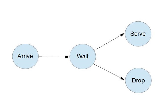
Figure 1: System job processing flow

We define a job as a tuple $J_{i}=<a_{i},b_{i},d_{i},w_{i},e_{i}>$.

• $a_{i},b_{i},d_{i}$ and $w_{i}$ are realizations of $A_{i},B_{i},D_{i}$ and $W_{i}$.

• $e_{i}=t_{i}+d_{i}$

Definition 2.

The cumulative reward function for time $t$ and policy $\pi$ is:

$$U_{t}^{\pi}=\sum\limits_{J_{i}\in S_{t}^{\pi}}w_{i}$$ (2)

Let $t=\hat{t}_{n}$ and $t^{\prime}=\hat{t}_{n-1}$ then, the reward difference function is:

$$\Delta U_{t}^{\pi}=U_{t}^{\pi}-U_{t^{\prime}}^{\pi}$$ (3)

The objective is to find a policy $\pi$ that maximizes the cumulative reward function. If the rewards are deterministic and $W_{i}=1$ the cumulative reward function measures the number of jobs that got service. If the rewards are $W_{i}=B_{i}$ the cumulative reward function measures the processing time utilization.

In Appendix -A queue behavior analysis is provided. As a result of this analysis, it is enough to examine the size of the queue potential and deduce the relationship between the corresponding size of $\hat{S}_{\hat{t}_{n}}^{\pi}$. Note that jobs that currently do not meet their deadline are disregarded here since they are not part of the queue potential.

III Scheduling Policies

In this section we describe several relevant scheduling policies which treat queues with priorities and deadlines.

III-A Earliest Deadline First

We define the EDF as follows: Let $t$ be the current time and assume that the queue is not empty and the server is ready to process a job.

The EDF was proved to be optimal under different metrics [16, 13, 9, 4]. Because of this optimality the EDF became the standard policy used in queuing models with deadlines.

Panwar, Towsley, and Wolf distinguish between service times being assigned (A-i) at arrivals or (A-ii) at beginning of services. Independently of when the assignment occurs, they assume that (A-iii) service times are not known to the scheduler at the beginning of the service. Then, they show that, under (A-iii), the two assignments (A-i) and (A-ii) are equivalent. In this paper, in contrast, we consider the case where (A-iii) does not hold (see assumption A1). Then, the distinction between (A-i) and (A-ii) is important. To illustrate that knowing the service times upon arrivals can lead can lead to improved results compared to EDF we consider the following variation on EDF which we term MEDF.

Assume that there are two jobs in the queue. $J_{1}$ has its expiration time at time 10 seconds and a service time of 30 seconds. $J_{2}$ has its expiration time at 20 seconds and a service time of 5 seconds. According to the EDF policy $J_{1}$ is processed before $J_{2}$. In this case $J_{2}$ is expired and is lost. If we change the order of $J_{1}$ and $J_{2}$ can be executed. Figure 2 depicts this case.

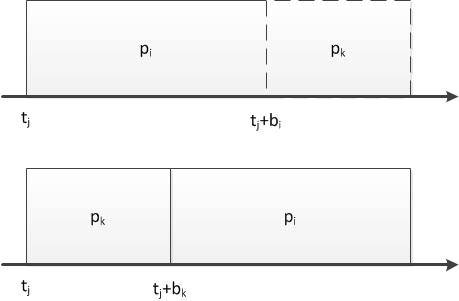
Figure 2: Example of queue order

The MEDF policy is a simple policy based on EDF but uses knowledge of the job reward and service time. It replaces the order of the first two jobs in the queue if this is beneficial. We introduce it here in order to present the advantages of using information on the service time.

Assume the current time is $t$. The queue has at least two jobs waiting and just finished processing a job and needs to choose a new job to process.

III-B $c\mu/\theta$ policy

Another policy which is relevant as a benchmark for testing our algorithm is the $c\mu/\theta$ scheduling policy [18]. The $c\mu/\theta$ policy assumes that are $K$ queues in the system where it needs to select the queue to be served. We assume that there are $K$ levels of rewards (or $K$ group of rewards) each against a queue. The $c\mu/\theta$ scheduling algorithm is composed of two steps:

1. Upon arrival the policy inserts the new job to queue $k$ according to its reward in FCFS order.

2. If the server becomes idle the policy chooses the queue to be served according to $c_{k}\mu_{k}/\theta_{k}$ and process the job that is in the head of the queue.

The $c\mu-rule$ was proven to be optimal in [35] assuming geometric service times and a preemptive scheduler. In [36] Bispo claimed that for convex costs, the optimal $c\mu-rule$ policy depends on the individual loads. He proposed first-order differences of the single stage cost function that reaches near optimal performances. In the non-preemptive case, the $c\mu-rule$ was proved to be optimal for the two-user case in [37]. The proof was done using calculus of variations arguments as well as an Infinitesimal Perturbation Analysis (IPA) approach. Down, Koole and Lewis [38] provided an optimal server assignment policy, under reward, linear holding costs, and a class-dependent penalty which reduces the reward for each customer that abandons the queue.

In our model we assume that the service times, deadlines and rewards are know upon arrival. The EDF assumes that there is no information about the service times, while in $c\mu/\theta$ the deadline is known statistically in terms of the probability of abandonment. This information has advantages in the case of a non-deterministic service time. We present a simple example showing the advantages of using knowledge of the service time upon arrival in the EDF case and present new version of $c\mu/\theta$ that exploits the knowledge of deadlines information. In the case of the $c\mu/\theta$ policy, knowing deadlines upon arrival allows us to modify the queue order to use EDF instead of FCFS as was proposed in [14]. We mark this new version as $c\mu/\theta E$. However, as we will show later our proposed technique outperforms this variation as well.

IV Maximum Utility with Dropping scheduling policy

We next present the Maximum Utility with Dropping (MUD) scheduling policy. The queuing model assumes SA1-SA6. We use the notation $\hat{S}_{t}^{M},\hat{Q}_{t}^{M},..$ to present the MUD parameters and $\hat{S}_{t}^{E},\hat{Q}_{t}^{E},..$ to present the EDF parameters.

The MUD policy combines both scheduling and dropping mechanisms. The scheduling algorithm is composed of two steps:

1. $\mbox{MUD}_{a}$ - Upon arrival the policy inserts the new job to the queue keeping the EDF order. If the insertion will cause a job to miss its deadline, the policy drops the packet with the minimal throughput ratio ($\frac{w_{i}}{b_{i}}$) from the queue.

2. $\mbox{MUD}_{s}$ - Upon terminating the service of a job the policy processes one of the two jobs in the head of the queue. The selected job is the one with the highest throughput ratio as long as it does not cause the second job to miss its deadline similarly to MEDF.

Let $o(J_{i},t)$ and $s(J_{i},t)$ be functions that characterize the queue potential order of $J_{i}$ with policy MUD at time $t$.

• $o(J_{i},t)$ is the index of job $J_{i}$ in $Q_{t}^{M}$. $o(J_{i},t)=1$ means that $J_{i}$ is at the head of the queue.

• $s(J_{i},t):=\sum\limits_{J_{k}:o(J_{k},t)<o(J_{i},t)}{b_{k}}$ is the time a job waits until it is processed assuming that no new jobs arrive until it starts processing.

Below we describe how the MUD policy handles a job arrival. Let $J_{i}$ be the new job which reaches to the queue $Q_{t_{i-1}}^{M}$ at time $t_{i}$.

Note that $o(J_{k},t_{i})$ and $s(J_{k},t_{i})$ values change after adding a new job $J_{i}$ at time $t_{i}$ as follows if $o(J_{k},t_{i})>o(J_{i},t_{i})$ then $s(J_{k},t_{i}):=s(J_{k},t_{i-1})+b_{i}$ and $o(J_{k},t_{i})=o(J_{k},t_{i-1})+1$ else there is no change. Different presentation of the policy is that it marks the jobs to drop at the arrival time and postpone the dropping stage to the time to the job reaches the head of the queue.

Next we analyze the complexity of adding a new job to a queue in the MUD policy. The MUD policy uses its dropping policy to maintain the queue in such a way that $\hat{Q_{t}}^{M}=Q_{t}^{M}$. According to formula 1 we can bound the queue size. Adding a job to the queue and dropping jobs from the queue require one sequential pass over the queue. Since the ratio $\frac{w_{m}}{b_{m}}$ is calculated upon arrival the policy only needs to compare $\frac{w_{m}}{b_{m}}$ and calculate the $s_{i}$. From the above we can conclude that the complexity of adding a job to the queue is bounded by the size of the queue potential as defined in 1.

In the FIFO policy the complexity of adding a new job is O(1). In the EDF policy the complexity of adding a new job is $O(\log(\max{|\hat{Q_{t}^{F}}|}))$ and in the CBS policy the complexity of adding a new job is $O(\max{|\hat{Q_{t}^{C}}|})$ with a calculation of the exponent and multiplication as described in [14]. The complexity of adding a new job to the queue in the MUD is larger than EDF but more efficient compared to the other policies. Using more complicated data structure the complexity can be reduced.

V MUD performance analysis

The following section presents the MUD performance analysis. This section analyzes the MUD scheduling policy performance in the $GI^{+}/D/1-GI^{+}/GI^{+}$ case. Then it proves the policy optimality in the $GI^{+}/D/1-GI^{+}/GI^{/}B+$ case.

V-A Deterministic Time Case

The analysis of the policies performance assumes that the queue becomes empty infinitely often. The assumption below forces this behavior.

1. $\mathbb{P}(A_{i}>D_{max})>0$.

Assumption A2 implies that there are infinitely many times where the queue is empty irrespective of the scheduling policy, i.e, for any two policies $\pi_{1}$ and $\pi_{2}$ there are $\tau_{1},\tau_{2},...\tau_{n},..$ times ($\tau_{n-1}<\tau_{n}$) which satisfy that both queues are empty; i.e. $Q_{\tau_{n}}^{\pi_{1}}=Q_{\tau_{n}}^{\pi_{2}}=\emptyset$.

Definition 3.

If $\forall n:U_{\tau_{n}}^{\pi_{1}}=U_{\tau_{n}}^{\pi_{2}}$ then policies $\pi_{1}$ and $\pi_{2}$ are equivalent.

Definition 4.

If $\mathbb{P}(\lim\limits_{n\rightarrow\infty}((U_{\tau_{n}}^{\pi_{1}}-U_{\tau_{n}}^{\pi_{2}})\geq 0)=1$ then $\pi_{1}$ is as good as $\pi_{2}$

Definition 5.

If $\mathbb{P}(\lim\limits_{n\rightarrow\infty}(U_{\tau_{n}}^{\pi_{1}}-U_{\tau_{n}}^{\pi_{2}})=\infty)=1$ then $\pi_{1}$ is better than $\pi_{2}$

Definition 6.

If for any policy $\pi_{2}$, $\pi_{1}$ is as good as policy $\pi_{2}$ then $\pi_{1}$ is optimal.

In the following section we analyze MUD performance against the group of policies that transmits the maximal number of packets. We show that MUD policy performance and the EDF policy performance in a $GI^{+}/D/1-GI^{+}/D$ is equal. In this model the service times and the rewards are deterministic (one unit) which is equivalent to the $GI^{+}/D/1-GI$ queuing model and the cumulative reward function is the number of processed jobs. In [16] it was shown that EDF policy is optimal in the terms of number of jobs to be processed for a queuing model satisfying $GI^{+}/D/1-GI$. We continue the analysis by showing that in a queuing model satisfying $GI^{+}/D/1-GI^{+}/GI^{+}$, the MUD policy is as good as the EDF policy or similar policies. We conclude with additional assumptions to show that the MUD policy is better than the EDF policy or similar policies.

Lemma 1.

For any queuing model satisfying $GI^{+}/D/1-GI^{+}/GI^{+}$, $\forall t:|Q_{t}^{M}|=|Q_{t}^{E}|$.

Proof.

Since the lemma is related solely to the number of jobs that are processed, the rewards are not used in the proof. The proof is based on the inequality between the two sides.

The first step is to prove that $\forall t:|Q_{t}^{M}|\leq|Q_{t}^{E}|$ .This inequality is derived from the optimality of EDF in a queuing model satisfying $GI^{+}/D/1-GI$ as was proven in [16].

For the other side $\forall n:|Q_{\hat{t}_{n}}^{M}|\geq|Q_{\hat{t}_{n}}^{E}|$ the proof is achieved by induction on $\hat{t}_{n}$. Let $t=\hat{t}_{n}$, the induction hypothesis is $|Q_{t}^{E}|=|Q_{t}^{M}|$ and the two policies provide service simultaneously (synchronized).

By definition at $n=0$ the queues are empty and the servers are idle $(Q_{t}^{E}=Q_{t}^{M}=\phi)$. At $n=1$ the first job arrives and is processed immediately by both policies, i.e., they are synchronized. This event is similar to all events when the queues are empty and the server is idle (QE1). By definition the service time is deterministic; thus the policies are synchronized as long as $Q_{t}^{E}$ and $Q_{t}^{M}$ have the same size. For the induction step, assume that the processing start time is synchronized and $|\hat{Q}_{t}^{M}|=|Q_{t}^{E}|=k$. We need to show that fot $t^{\prime}=\hat{t}_{n+1}$, $|Q_{t^{\prime}}^{M}|=|Q_{t^{\prime}}^{E}|$ is kept, and the service start time is synchronized in the following cases:

• Begin processing a job in one or both policies (QE3)

• Arrival of a new job when the server is busy (QE2)

First we analyze the case of QE3. Let $|Q_{t}^{E}|=|Q_{t}^{M}|>0$. When the event of process begins $\Delta Q_{t^{\prime}}^{E}=\Delta Q_{t^{\prime}}^{M}=-1$ . The processing begins simultaneously (induction hypothesis) and since the processing time is deterministic, both policies end processing simultaneously , thus adhering to the induction hypothesis.

Second we analyze the case of QE2. As stated above QE2 contains two type of events: QE2a when the new job is added to the queue potential and the queue potential is growing and QE2b when the new job causes one of the jobs in the queue potential to miss its deadline.

The arrival of a new job does not impact the synchronization of the processing. We analyze events QE2a and QE2b in both policies.

1. Similar behavior of the two policies in the event QE2a.

2. Similar behavior of the two policies in the event QE2b.

3. $\Delta Q_{t^{\prime}}^{E}=0,\Delta Q_{t^{\prime}}^{M}=1$, MUD event is QE2a while the EDF event is QE2b.

4. $\Delta Q_{t^{\prime}}^{E}=1,\Delta Q_{t^{\prime}}^{M}=0$, MUD event is QE2b while the EDF event is QE2a.

The first two cases preserve the induction hypothesis as required. The third case contradicts the optimality of the EDF; in other words the event cannot exist. We show that the fourth event cannot exist.

By definition $Q_{t}^{M}\subseteq\hat{Q}_{t}^{E}$ since they have the same feed of jobs and the queues are ordered by expiration time. Let $J_{j}$ be the job that is dropped by the MUD policy at time $t$. If $J_{j}\in Q_{t}^{E}$, then, there are more jobs in $Q_{t}^{M}$ then in $Q_{t}^{E}$ whose expiry time is less than $e_{j}$. This contradicts the optimality of EDF (please note that the order of the queues is the same). If $J_{j}\notin Q_{t}^{E}$ since $e_{j}\geq e_{i}$ we can add it to $Q_{\hat{t}_{n-1}}^{E}$ without dropping and have a larger queue since $J_{i}$ is added at time $t_{i}$. This contradicts the optimality of EDF. This means that case 4 cannot exist. The result is that the processing is synchronized and the queues have a similar size. ∎

Lemma 2.

For any queuing model satisfying $GI^{+}/D/1-GI^{+}/D$, the MUD and the EDF policies are equivalent.

Proof.

Since the reward is deterministic, without loss of generality assume $W_{i}=1$. Therefore, from lemma 7 and lemma 1 we get that $\forall t:U_{t}^{E}=|\hat{S}_{t}^{E}|=|\hat{S}_{t}^{M}|=U_{t}^{M}$ thus MUD and EDF are equivalent. ∎

Theorem 1.

For any queuing model satisfying $GI^{+}/D/1-GI^{+}$, the MUD policy is optimal in terms of the number of jobs to process where the process time is exactly one unit.

Proof.

Queuing models satisfying $GI^{+}/D/1-GI^{+}/D$ are equivalent to queuing systems satisfying $GI^{+}/D/1-GI$ if we measure the number of jobs that were processed and $W_{i}=1$. In the case of a deterministic service time, knowing the service time upon arrival or just before service is equivalent since both are known to be a constant. In [16] it was shown that the EDF policy is optimal in terms of the number of jobs to process for the discrete time $GI^{+}/D/1-GI$ queue where process time is exactly one unit. In lemma 2 we showed that the MUD is equivalent to EDF; thus MUD is optimal in terms of the number of jobs to process where the process time is exactly one unit and the reward is also one unit. ∎

Let $\mathcal{M}$ be the group of policies that processes the maximal number of jobs assuming $GI^{+}/D/1-GI^{+}/GI^{+}$. $EDF,MUD\in\mathcal{M}$ as a result of [16] and Lemma 2 . Let $\mathcal{M}_{E}\subseteq\mathcal{M}$ be the group of policies that their expected reward is $E(W_{i})$.

In order to prove lemma 3 we add the following assumptions:

1. $A_{i}$, $D_{i}$ and $W_{i}$ have discrete probability distribution function.

2. $A_{i},D_{i}$ and $W_{i}$ are independent of each other.

Assumption A3 is used to simplify the proofs. In addition $W_{i}$ has finite presentation in the communication environment forcing discrete distribution. $A_{i}$ and $D_{i}$ may have a continuous distribution function as well. Assumption A4 is reasonable since $A_{i}$ is related to the server’s arrival process. $D_{i}$ is derived from the original deadline reducing different network delays. $W_{i}$ is generated independently by the data source.

Lemma 3.

For any queuing model satisfying $GI^{+}/D/1-GI^{+}/GI^{+}$ and assumptions A2-A4, MUD policy is as good as EDF.

Proof.

This proof analyzes the behavior of the different types of events. For purposes of this proof let $\pi\in\{MUD,EDF\}$ and let $t=\hat{t}_{n}$ the time of event $\mathcal{E}_{n}^{\pi})$ and $t^{\prime}=\hat{t}_{n-1}$ the time of event $\mathcal{E}_{n-1}^{\pi}$ be the times of the current event and the prior event. The different cases are:

1. Arrival of a new job at events QE1 and QE2 where $\Delta Q_{t}^{E}\neq\Delta Q_{t}^{M}$. This contradicts Lemma 1 since one of the $Q_{t}^{\pi}$ becomes longer than the other one.

2. Arrival of a new job where $\Delta Q_{t}^{E}=\Delta Q_{t}^{M}=1$ (QE2a). In this case a job was added to both queue potentials without reducing the number of jobs in them. The queue potential reward growth is the same in both queues.

3. Arrival of a new job where $\Delta Q_{t}^{E}=\Delta Q_{t}^{M}=0$ (QE2b). In this case there is a change in the queue potential rewards which can be different between policies.

4. Processing begins of a job in one or both policies (QE3) - Process starting moves the job from $Q_{t^{\prime}}^{\pi}$ to $\hat{S}_{t}^{\pi}$ keeping $S_{t^{\prime}}^{\pi}=S_{t}^{\pi}$.

5. A job does not meet its deadline (QE4) or is dropped (QE5) - By definition this job did not belong to $S_{t^{\prime}}^{\pi}$.

We define $\Delta U_{t}^{\pi}$ explicitly and compare the difference between the two policies. For arrival events QE1, QE2a and QE2b let $J_{i}$ be the arriving job and $t=\hat{t}_{n}=t_{i}$ be the current time. We use $W_{j}^{E}$ or $W_{k}^{M}$ to describe the rewards of jobs $J_{j}$ and $J_{k}$ that are removed or dropped from the queue potentials in the different policies.

Let $\Delta U_{t}^{\pi}$ be:

$$\Delta U_{t}^{E}=\begin{cases}0&\text{Events \ref{QE5}, \ref{QE6} and \ref{QE7}}\\ W_{i}&\text{Events \ref{QE1}, \ref{QE3}}\\ W_{i}-W_{j}^{E}&\text{Event \ref{QE4}}\end{cases}$$ (4)

$$\Delta U_{t}^{M}=\begin{cases}0&\text{Events \ref{QE5}, \ref{QE6} and \ref{QE7}}\\ W_{i}&\text{Events \ref{QE1}, \ref{QE3}}\\ W_{i}-W_{k}^{M}&\text{Event \ref{QE4} and }W_{k}^{M}<W_{i}\\ 0&\text{Event \ref{QE4} and }W_{k}^{M}\geq W_{i}\end{cases}$$ (5)

We are interested in the difference between the potential rewards, $\Delta U_{t}^{M}$ and $\Delta U_{t}^{E}$. In the events QE1, QE2a, QE3, QE4 and QE5, $\Delta U_{t}^{M}=\Delta U_{t}^{E}$ as was presented above. We focus on the behavior of events of type QE2b which impacts the queue potential rewards.

Let $\tau=\{\tau_{1},\tau_{2}...\}$ be a sequence of times satisfying QE2b and let $t_{i}=\tau_{m}$. Let $\hat{\mathbb{E}}(W_{i})$ be the empirical mean of the sequence of all events of type QE2b up to time $\tau_{m}=t_{i}$.

We begin by analyzing the queue potential behavior in the EDF. In this event an arbitrary job from $Q_{t_{i-1}}^{E}\cup\{J_{i}\}$ misses its deadline and is removed from the queue potential. The EDF policy orders the queue according to expiration time. Hence the job that misses its deadline only depends on its deadline. Since the deadlines and the rewards are independent according to assumption A4 and rewards are i.i.d we get:

$$\begin{split}\lim\limits_{m\rightarrow\infty}\hat{\mathbb{E}}&(\Delta U_{\tau_{m}}^{E})=\lim\limits_{m\rightarrow\infty}\hat{\mathbb{E}}(W_{i}-W_{j}^{E})\\ &=\lim\limits_{m\rightarrow\infty}\hat{\mathbb{E}}(W_{i})-\lim\limits_{m\rightarrow\infty}\hat{\mathbb{E}}(W_{j}^{E})\\ &\xrightarrow{a.s}\mathbb{E}(W_{i})-\mathbb{E}(W_{j})=0\end{split}$$ (6)

This means that $EDF\in\mathcal{M}_{E}$.

On the other hand the MUD policy drops a job with the minimal reward from $Q_{t^{\prime}}^{M}\cup\{J_{i}\}$ as defined in statements 5-8 of the policy. Let $J_{k}^{M}$ be the job that is chosen to be dropped in the MUD case. Let $n$ be the number of events in sequence $\tau$ which occur up to event $t_{i}$.

$$\begin{split}\hat{\mathbb{E}}(\Delta U_{\tau_{m}}^{M})&=\frac{1}{m}\sum\limits_{i\leq m}\Delta U_{\tau_{\hat{i}}}^{M}\\ &=\frac{1}{m}(\sum\limits_{\hat{i}\leq m:W_{k}\geq W_{i}}\Delta U_{\tau_{\hat{i}}}^{M}+\sum\limits_{\hat{i}\leq m:W_{k}<W_{i}}U_{\tau_{\hat{i}}}^{M})\\ &=\frac{1}{m}\sum\limits_{\tau_{\hat{i}}\leq\tau_{m}:W_{k}<W_{i}}U_{\tau_{\hat{i}}}^{M}\geq\frac{1}{m}\sum\limits_{\tau_{\hat{i}}\leq\tau_{m}:W_{k}<W_{i}}\delta_{W}\geq 0\end{split}$$ (7)

If $\lim\limits_{m\rightarrow\infty}\hat{\mathbb{E}}(\Delta U_{\tau_{m}}^{M})\xrightarrow{a.s}0$ then the probability of the event that $W_{k}<W_{i}$ in the sequence is 0; i.e., that the number of beneficial exchanges achieved by the MUD is negligible. The MUD policy orders the queue by expiration time exactly like EDF; thus, both policies behave identically at probability 1. Alternatively $\lim\limits_{m\rightarrow\infty}\hat{\mathbb{E}}(\Delta U_{m}^{E})\xrightarrow{a.s}\epsilon>0$.

The conclusion is that the MUD policy is at least as good as the EDF policy. ∎

Theorem 2.

For any queuing model satisfying $GI^{+}/D/1-GI^{+}/GI^{+}$ and assumptions A2-A4 , MUD policy is as good as any policy $\pi\in\mathcal{M}_{E}$.

Proof.

By definition $\forall\pi\in\mathcal{M}_{E}:$ their expected reward is $E(W_{i})$. From Dertouzos theorem [4] we know that EDF is optimal in that if there exists any policy $\pi$ that can build a feasible schedule then EDF also build a feasible schedule. Adding to it lemma 3 we deduce that MUD policy is as good as any policy $\pi\in\mathcal{M}_{E}$. ∎

In order to prove that the MUD policy is better than any policy $\pi\in\mathcal{M}_{E}$ the following assumptions are required:

1. $\mathbb{P}(B_{i}<D_{max})>0$.

2. $\exists\delta>0:\mathbb{P}(A_{i}=B_{min}-\delta)>0$, Let $A_{\delta}=B_{min}-\delta$

3. $\mathbb{V}ar(W_{i})\neq 0$.

4. Let $\delta_{W}$ be the minimal difference between two different rewards. A3 and A7 imply that $\delta_{W}>0$.

Assumption A5 guarantees that there is always a positive probability that a feasible job arrives. This is a natural assumption, since otherwise the will be no jobs to process. Assumption A6 guarantees that jobs wait in the queue with positive probability irrespective of the scheduling policy. A8 always holds when $W_{i}$ has a discrete distribution with finite support.

Lemma 4.

For any queuing model satisfying $GI^{+}/D/1-GI^{+}/GI^{+}$ and assumptions A1 - A8, there exists an arrival $\hat{\mathcal{A}}_{j(n+2)}^{\pi}=\{\ref{QE4}\}$ which occurs infinitely often such that $\Delta U_{t_{j(n+2)}}^{M}=\delta_{W}$.

Proof.

In order to prove the lemma we generate a sequence of job arrivals called $\tilde{\mathcal{A}}_{i}^{\pi}\subset\mathcal{A}$ with strictly positive probability. We prove that the last event of sequence is of type QE2b regardless the scheduling policy. The sequence of jobs is defined as follows:

1. Let $J_{i}=<a_{i},1,D_{max},W_{min},t_{i}+D_{max}>$ where $a_{i}>D_{max}$ be the first job in the sequence.

2. Let $\{<A_{\delta},1,D_{max},W_{min},t_{k}+D_{max}>\}_{k=i+1}^{i+n}$ be a sequence of $n$ jobs with constant parameters. Let $n$ be defined by:

   $$n=\lceil\frac{\ D_{max}}{\delta}\rceil$$ (8)

3. Let $J_{i+n+1}=<A_{\delta},1,D_{max},W_{max},t_{i+n+1}+D_{max}>$ be the last job in the sequence.

The first arrival empties the queue potential with positive probability by assumption A2. By assumption A5, if $a_{k}=A_{\delta}$ the queue is increased upon arrival of $J_{k}$. After $n+1$ arrivals there is at least one job waiting in the queue when $J_{i+n+1}$ arrives. Meaning that one job must miss its deadline ($\Delta Q_{\tau_{i+n+1}}^{\pi}=0$). The probability of the arrival of $J_{k}\in\{<A_{\delta},1,D_{max},W_{min},t_{k}+D_{max}>\}_{k=i+1}^{i+n}$ is $\mathbb{P}(A_{i}=A_{\delta})\mathbb{P}(D_{i}=D_{max})\mathbb{P}(W_{i}=W_{min})>0$ due to assumption A4. The probability of the arrival of $J_{i+n+1}$ is $\mathbb{P}(A_{i}=A_{\delta})\mathbb{P}(D_{i}=D_{max})\mathbb{P}(W_{i}=W_{max})>0$. As a result the event $\hat{\mathcal{A}}_{i}^{\pi}$ has positive occurrence probability since:

$$\begin{split}\mathbb{P}(\tilde{\mathcal{A}}_{k})&=\mathbb{P}(A_{i}>D_{max})[\mathbb{P}(A_{i}=A_{\delta})\mathbb{P}(D_{i}=D_{max})\\ &\mathbb{P}(W_{i}=W_{min})]^{n}\mathbb{P}(A_{i}=A_{\delta})\mathbb{P}(D_{i}=D_{max})\\ &\mathbb{P}(W_{i}=W_{max})>0\end{split}$$ (9)

The MUD policy drops a job with a smaller reward than $J_{i+n+1}$ causing the cumulative reward functions to increase at least by $\delta_{W}$. For comparison, the EDF policy drops $J_{i+n+1}$ because it misses its deadline.

The arrivals are independent and mutually exclusive events by definition (forcing an empty queue) and $\sum\limits_{j=1}^{\infty}\mathbb{P}(\hat{\mathcal{A}}_{j(n+2)}^{\pi})=\infty$. By the second Borel Cantelli lemma, $\mathbb{P}(\limsup\limits_{j\rightarrow\infty}\hat{\mathcal{A}}_{j(n+2)}^{\pi})=1$; i.e., meaning that this event occurs infinitely often.

∎

From lemma 4 the series of events of type $\hat{\mathcal{A}}_{i}$ satisfies:

$$\Delta U_{t_{i}}^{M}-\Delta U_{t_{i}}^{E}\geq\delta_{W}$$ (10)

Theorem 3.

For any queuing model $GI^{+}/D/1-GI^{+}/GI^{+}$ satisfying assumptions A1 - A8, MUD policy is better than any policy $\pi\in\mathcal{M}_{E}$.

Proof.

From theorem 2 we know that $\Delta U_{t}^{M}=\Delta U_{t}^{E}$ in all cases except QE2b case and that $\lim\limits_{n\rightarrow\infty}\hat{\mathbb{E}}(\Delta U_{\tau_{n}}^{E})\xrightarrow{a.s}0$. in case QE2b. From lemma 4 we can conclude as regards QE2b that $\lim\limits_{i\rightarrow\infty}\sum\limits_{\tau_{i}}\Delta U_{\tau_{i}}^{E}=\infty$. By the strong law of large numbers there exists an $n_{0}$ that for all $n>n_{0}:\hat{\mathbb{E}}(\Delta U_{\hat{t}_{n}}^{E})<\frac{\delta_{W}\mathbb{P}(\hat{\mathcal{A}}_{k})}{3}$ with probability 1. Let $C=-\sum\limits_{m\leq n_{0}:\tau_{m}\in\tau}U_{\hat{t}_{m}}^{E}$. Then

$$\begin{split}U_{\hat{t}_{n}}^{M}&-U_{\hat{t}_{n}}^{E}\geq C+\sum\limits_{n\geq m\geq{n_{0}}}(\Delta U_{\hat{t}_{m}}^{M}-\Delta U_{\hat{t}_{m}}^{E})\\ &=C+\sum\limits_{n_{0}\leq m\leq n:\hat{t}_{m}\not\in\tau}(\Delta U_{\hat{t}_{m}}^{M}-\Delta U_{\hat{t}_{m}}^{E})\\ &\geq C+\sum\limits_{n_{0}\leq m\leq n:\hat{t}_{m}\in\tau}(\Delta U_{\hat{t}_{m}}^{M}-\Delta U_{\hat{t}_{m}}^{E})\end{split}$$ (11)

$$\begin{split}\lim\limits_{n\rightarrow\infty}(U_{t_{n}}^{M}-U_{t_{n}}^{E})&\geq\\ &C+\lim\limits_{n\rightarrow\infty}\sum\limits_{n_{0}\leq m\leq n:\hat{t}_{m}\in\tau}(\Delta U_{\hat{t}_{m}}^{M}-\Delta U_{\hat{t}_{m}}^{E})\\ &\geq C+\lim\limits_{n\rightarrow\infty}(n-n_{0})\frac{\delta_{W}\mathbb{P}(\hat{\mathcal{A}}_{k})}{3}\xrightarrow{a.s}\infty\end{split}$$ (12)

This means that the MUD policy is better than EDF policy when assumptions A1 - A8 are held. Adding to it Dertouzos theorem [4] we can deduce that MUD policy is better than any policy $\pi\in\mathcal{M}_{E}$. ∎

V-B Deterministic Time and Dual Reward Case

In this section we study the optimality of the MUD policy for deterministic service time. To simplify an already complicated notation we focus on the two priority levels case. We define a dual reward process by $W_{i}\in\{w_{min},w_{max}:w_{min}<w_{max}\}$ i.e. $(W_{i}\sim\mathcal{B}(p))$.

In the dual reward case we can split the queue into two sub-queues. Let

• ${\color[rgb]{0,0,0}Q_{i}^{M(max)}}=\{w_{j}\in Q_{i}^{M}:w_{j}=w_{max}\}$ be the set of jobs in the queue potential with maximal reward.

• ${\color[rgb]{0,0,0}Q_{i}^{M(min)}}=\{w_{j}\in Q_{i}^{M}:w_{j}=w_{min}\}$ be the set of jobs in the queue potential with minimal reward.

Similarly, we split the group of processed jobs to two groups:

• ${\color[rgb]{0,0,0}\hat{S}_{i}^{M(max)}}=\{w_{j}\in\hat{S}_{i}^{M}:w_{j}=w_{max}\}$ be the set of processed jobs with maximal reward.

• ${\color[rgb]{0,0,0}\hat{S}_{i}^{M(min)}}=\{w_{j}\in\hat{S}_{i}^{M}:w_{j}=w_{min}\}$ be the set of processed jobs with maximal reward.

Let $R_{i}^{M(max)}=|Q_{i}^{M(max)}\cup\hat{S}_{i}^{M(max)}|$ be the number of jobs with maximal reward in the queue potential and in the group of processed jobs.

We say that $R_{i}^{M(max)}$ is optimal if no other policy can process more jobs with maximal rewards than $R_{i}^{M(max)}$. For the proofs in this section we assume the following:

One of the major problems in non-preemptive scheduling without idle time is the problem of priority inversion [4]. To overcome this problem we add the following assumption:

1. Let $D_{min}>2B_{max}$ meaning that the deadline is at least twice the time required for processing the longest packet.

For non-border routers in a network this assumption is reasonable since it allows the packets to reach their destination.

First we show that the mild inversion of two packets at the Queue head in $\mbox{MUD}_{s}$, does not cause drops of other packets.

Lemma 5.

Let $J_{l},J_{k}\in Q^{M}_{i}:o(J_{l},t_{i})=1$ and $o(J_{k},t_{i})=2$ and assume A9, then replacing the service order of $J_{l},J_{k}$ does not impact the MUD performance.

Proof.

In order to prove the lemma we need to show that for all packets that their order in the queue is higher than 2 ($o(J_{i},t)>2$) their expected service time $s(J_{i},t)$ is kept. By definition $s(J_{i},t):=\sum\limits_{J_{k}:o(J_{k},t)<o(J_{i},t)}{b_{k}}=\sum\limits_{J_{k}:2<o(J_{k},t)<o(J_{i},t)}{b_{k}}+\sum\limits_{J_{k}:o(J_{k},t)\leq 2}{b_{k}}$. Since $\sum\limits_{J_{k}:o(J_{k},t)\leq 2}{b_{k}}$ is kept regardless the processing order the $s(J_{i},t)$ is kept. Assumption A9 eliminates the possibility that the replacement causes packet to miss its deadline due to a new arrival. This means that assuming A9 the replacement in the head of the queue does not impact the MUD performance. ∎

Lemma 6.

For any queuing model $GI^{+}/D/1-GI^{+}/GI^{/}B+$ satisfying assumption A9, $R_{i}^{M(max)}$ is optimal.

Proof.

The main idea behind the proof is that under MUD $Q_{i}^{M(max)}$ behaves like EDF queue of maximal reward jobs. Jobs with minimal reward are processed by MUD only if they do not impact jobs with maximal reward and close to their expiration time. Since we already proved that MUD processes the maximal number of packets as well as the maximal number of packets with highest priority, it must be optimal. We wish to prove by induction that $R_{i}^{M(max)}$ is optimal. For $t_{0}$ it is true since $R_{i}^{M(max)}=0$. Assume by induction that $R_{i-1}^{M(max)}$ is optimal, we wish to prove that it is optimal for $R_{i}^{M(max)}$, we prove it per event type;

1. Event QE1 the job is processed in all policies. Since no other policy can do better, $R_{i}^{M(max)}$ is optimal ($R_{i}^{M(max)}=R_{i-1}^{M(max)}+1$).

2. Event QE2a the job is added to the queue potential without a drop. Since no other policy can do better, $R_{i}^{M(max)}$ is optimal ($R_{i}^{M(max)}=R_{i-1}^{M(max)}+1$).

3. Event QE2b. The event happens also in any other policy as well due to the optimality of the MUD by theorem 1. Let $J_{i}$ be the arriving job. The event is divided into two cases:

   • MUD marks for dropping a job with minimal reward - If the new job has a maximal reward then $R_{i}^{M(max)}=R_{i-1}^{M(max)}+1$ otherwise $R_{i}^{M(max)}=R_{i-1}^{M(max)}$. Since no other policy can do better, $R_{i}^{M(max)}$ is optimal.

   • MUD marks for dropping a job with maximal reward - this happens only if the new job has a maximal reward. Assume by negation that exists a policy that drops job with minimal reward instead. We can take it’s queue potential and MUD queue potential and extract out of them a new queue potential which has more jobs with maximal reward than the induction assumption. This contradict the induction assumption. Since no other policy can do better, $R_{i}^{M(max)}$ is optimal.

4. Event QE3 this event does not impact $R_{i}^{M(max)}$ directly but through event QE2b. MUD postpones as much as possible giving service to jobs with minimal reward in order to maximize the event of dropping job with minimal reward at event QE2b. Lemma 5 states that the replacement does not impact the queue potential assuming A9.

5. Events QE4 and QE5 do not impact $R_{i}^{M(max)}$.

We proved that $R_{i}^{M(max)}$ is optimal. ∎

From lemma 6 we can conclude that at times $Q_{i}^{M}=\emptyset$, $\hat{S}_{i}^{M(max)}$ is optimal.

Theorem 4.

For any queuing model $GI^{+}/D/1-GI^{+}/B$ satisfying assumption A9, MUD policy is optimal.

Proof.

To prove the theorem we need to show that at times $Q_{i}^{M}=\emptyset$, $U^{M}_{t_{i}}$ is optimal .

Let $N_{i}^{M}$ be the number of jobs process by policy MUD until time $t_{i}$.

$$U_{t_{i}}^{M}=\sum\limits_{J_{l}\in S_{t_{i}}^{M}}w_{l}=R_{i}^{M(max)}W_{max}+(N_{i}^{E}-R_{i}^{M(max)})W_{min}$$ (13)

In theorem 1 we proved that $N_{i}^{M}$ is optimal and in lemma 6 we proved that $R_{i}^{M(max)}$ is optimal. Hence $U_{t_{i}}^{M}$ includes both the maximal number of packets and maximal number of packets with highest rewards. This implies that no other policy can do better. ∎

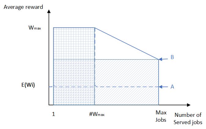
Figure 3: Pareto optimality graph -
Jobs counting is ordered by descending rewards

Figure 3 depicts the behavior of different policies in respect to the number of served jobs and the estimated reward. Point A presents the performance of policies in $\mathcal{M}_{E}$. MUD performance is between point $A$ and $B$. In the dual reward case we proved that MUD performance is at point B. The area in the graph depicts the total reward accumulated by the policy. We prove that MUD is optimal in the dual reward case concluding that its rectangle has the maximal area.

Similar analysis shows the following theorem for two packet sizes with equal rewards:

Theorem 5.

For any queuing model $GI^{+}/B/1-GI^{+}/D$ satisfying A9, MUD policy is optimal.

This result has both practical and theoretical interest. While EDF is not optimal for non-deterministic service time, we can extend the optimality of MUD to the case of dual service times when there are no rewards. Furthermore, in practice in many cases we have data packets of fixed length (typical in Ethernet) and acknowledgment packets which are much shorter. Assuming a sufficient reception window for ACK packets, the MUD policy is indeed optimal.

V-C Non-deterministic Service Time

The problem of ordering non-deterministic service time queues without preemption is similar to be optimization problems which their complexity is $NP-hard$ [6]. In addition, if avoiding assumption A9 policies that do not force idle cannot achieve optimality due to priority inversion problem [4]. In the next section we present simulation of the non-deterministic service time and compare the policies we discussed.

VI Numerical Results

In this section we present the numerical results of simulations comparing the the performance of EDF, CBS, MUD, two versions of $c\mu_{k}/\theta_{k}$ and $Greedy$ policy. For the $c\mu_{k}/\theta_{k}$ we allocated a queue per reward. We used linear cost function that is based on the queue reward (4 or 10) multiplied by the length of the queue. Since the $c\mu_{k}/\theta_{k}$ policies do not take advantage of all at the knowledge of the deadline we introduced a new version of the $c\mu_{k}/\theta_{k}$ that instead of ordering the queue by FCFS it orders the jobs using EDF and called it $c\mu/\theta_{E}$. We also compare the results with a greedy algorithm that process the job with the highest reward. In the following simulation we tested the M/M/1-M/B case. We ran 100,000 samples with the following parameters:

• $A$ - is exponentially distributed with $\lambda_{a}=0.9,1.2,1.5,1.8,2.1$

• $B$ - is exponentially distributed with $\lambda_{b}=1$

• $D$ - is exponentially distributed with $\lambda_{d}=0.005$

• $E$ - is distributed $\mathcal{B}(0.5)$ with probability $p$ the reward is 10 and with probability $1-p$ the reward is 4.

Figure 4 presents the reward collection of the different policies. Figure 5 presents the number of jobs that were processed. The results are shown relative to the baseline of the EDF policy.

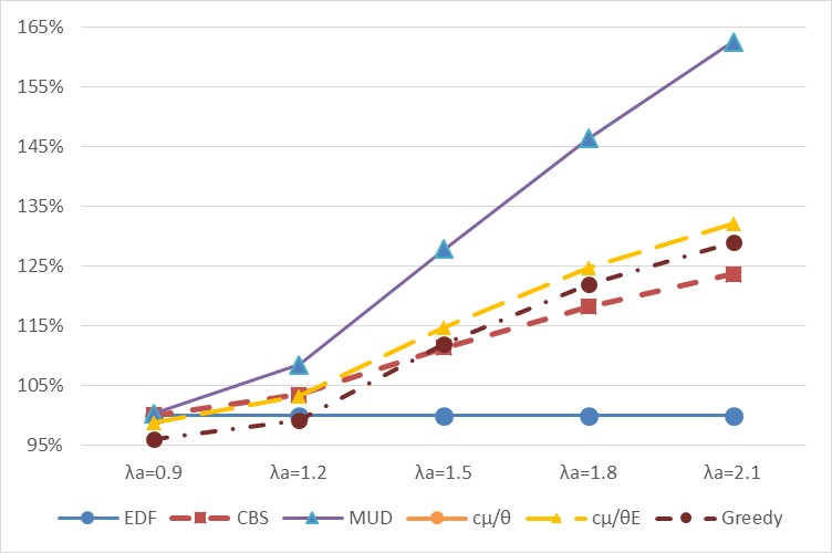
Figure 4: Collected rewards M/M/1-M/B case

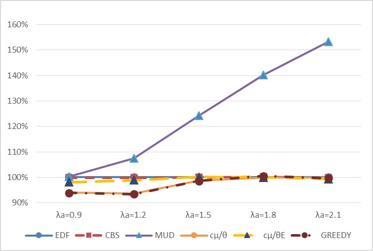
Figure 5: Number of processed Jobs M/M/1-M/B case

In the next simulation we tested the M/M/1-M/M case. We ran 100,000 samples with the following parameters:

• $A$ - is exponentially distributed with $\lambda_{a}=0.9,1.2,1.5,1.8,2.1$

• $B$ - is exponentially distributed with $\lambda_{b}=1$

• $D$ - is exponentially distributed with $\lambda_{d}=0.005$

• $E$ - is exponentially distributed with $\lambda_{e}=0.1$.

Figure 4 presents the reward collection of the different policies. Figure 5 presents the number of jobs that were processed. The results are shown relative to the baseline of the EDF policy.

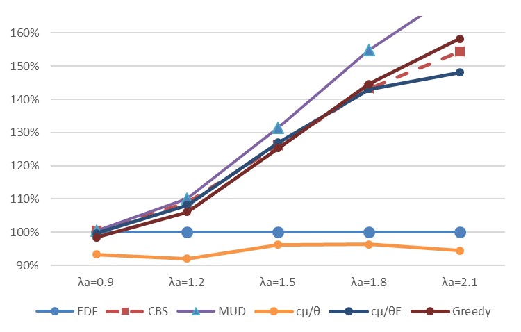
Figure 6: Collected rewards M/M/1-M/M case

Figure 7: Number of processed Jobs M/M/1-M/M case

In both simulations we clearly see that MUD performs better than other policies. It processes many more packets and the total collected reward is significantly higher than other policies. We see also that MUD outperforms when the number of overrun increases due to higher ration between the arrival rate and the service rate ($\rho$).

VII Conclusion

We presented a novel scheduling policy that takes advantage of knowing the job parameters upon arrival. We proved that the policy is optimal under deterministic service time and binomial reward distribution. In the more general case we proved that the policy processes the maximal number of packets while collecting rewards higher than the expected reward. We present simulation results that show its high performance in more generic cases while keeping computational demands low.

-A Queue Behavior Analysis

In this annex a queue behavior analysis of a simple model satisfying $GI^{+}/D/1-GI^{+}/GI^{+}$ is provided. Assume that the current time is $t=t_{i}=\hat{t}_{n}$ and $t^{\prime}=\hat{t}_{n-1}$.

1. Job $J_{i}$ reaches the system while the server is idle and the queue is empty - In this case $J_{i}$ is processed immediately. The queue and the queue potential are kept empty $\hat{Q}_{t}^{\pi}=Q_{t}^{\pi}=\emptyset$ and $\Delta Q_{t}^{\pi}=0$. $S_{t}^{\pi}=\hat{S}_{t}^{\pi}=S_{t^{\prime}}^{\pi}\cup\{J_{i}\}$. $\Delta U_{t}^{\pi}=w_{i}$ and $U_{t}^{\pi}=U_{t^{\prime}}^{\pi}+w_{i}$.

2. Job $J_{i}$ reaches the system while the server is busy - In this case $J_{i}$ waits in the queue, $\hat{Q}_{t}^{\pi}=\hat{Q}_{t^{\prime}}^{\pi}\cup\{J_{i}\}$ and $\hat{S}_{t}^{\pi}=\hat{S}_{t^{\prime}}^{\pi}$. The arrival of a job may impact the queue potential $Q_{t}^{\pi}$ differently according to the parameters of the job and the way the policy arranges the queue. This can cause the following two events:

   1. If $\Delta Q_{t}^{\pi}=1$ the job joins the queue potential, $Q_{t}^{\pi}=Q_{t^{\prime}}^{\pi}\cup\{J_{i}\}$ and $\Delta U_{t}^{\pi}=w_{i}$ .

   2. If $\Delta Q_{t}^{\pi}=0$, i.e., the queue potential size does not change. This is a result of either not adding the arriving job to the queue potential or removing a different job from the queue potential because it missed its deadline. Assume $J_{j};j\leq i$ is the job removed from the queue potential, then $Q_{t}^{\pi}=Q_{t^{\prime}}^{\pi}\cup\{J_{i}\}-\{J_{j}\}$ and $\Delta U_{t}^{\pi}=w_{i}-w_{j}$ .

   3. Job $J_{i}$ reaches the system while the server is busy and $\Delta Q_{\hat{t}_{n}}^{\pi}<0$. This event cannot take place since the service time is deterministic and there is only a replacement of jobs.

3. Job $J_{j}$ where $j<i$ begins process. In this case $\hat{Q}_{t}^{\pi}=\hat{Q}_{t^{\prime}}^{\pi}-\{J_{j}\}$, $Q_{t}^{\pi}=Q_{t^{\prime}}^{\pi}-\{J_{j}\}$, $\Delta Q_{t}^{\pi}=-1$, $S_{t}^{\pi}=S_{t^{\prime}}^{\pi}$, $\hat{S}_{t}^{\pi}=\hat{S}_{t^{\prime}}^{\pi}\cup\{J_{j}\}$ and $\Delta U_{t}^{\pi}=0$.

4. Deadline expired for $J_{j}$ - This event does not impact the variables that describe the system. $J_{j}$ is kept in the queue. $Q_{t}^{\pi}$ is not impacted since $J_{j}\notin Q_{t}^{\pi}$. $\hat{S}_{t}^{\pi}=\hat{S}_{t^{\prime}}^{\pi}$ as well as $S_{t}^{\pi}=S_{t^{\prime}}^{\pi}$.

5. Drop of job $J_{j}$. The drop means that the job was removed from the queue i.e $\hat{Q}_{t}^{\pi}=\hat{Q}_{t^{\prime}}^{\pi}-\{J_{j}\}$. If $J_{j}\in Q_{t^{\prime}}^{\pi}$ then $\Delta Q_{t}^{\pi}=-1$ and $\Delta U_{t}^{\pi}=-w_{j}$.

Next we prove the relationship between $Q_{t}^{\pi}$ and $\hat{S}_{t^{\prime}}^{\pi}(t^{\prime}\leq t)$.

Lemma 7.

For any queuing model satisfying $GI^{+}/D/1-GI^{+}/GI^{+}$, two policies $\pi_{1},\pi_{2}$ and times $t=\hat{t}_{n}$, $t^{\prime}=\hat{t}_{m}$ ($\hat{t}_{n}$ and $\hat{t}_{m}$ are the times of $\mathcal{E}_{n}^{\pi_{1}}$ and $\mathcal{E}_{m}^{\pi_{1}}$ ) : if $\forall t,t^{\prime}$ and $t\geq t^{\prime}:|Q_{t^{\prime}}^{\pi_{1}}|\geq|Q_{t^{\prime}}^{\pi_{2}}|$ then $|\hat{S}_{t}^{\pi_{1}}|\geq|\hat{S}_{t}^{\pi_{2}}|$.

Proof.

Assume by negation that there exists $t$ such that $\forall t^{\prime}\leq t:|Q_{t^{\prime}}^{\pi_{1}}|\geq|Q_{t^{\prime}}^{\pi_{2}}|$ but $|\hat{S}_{t}^{\pi_{1}}|<|\hat{S}_{t}^{\pi_{2}}|$ . We take the minimal $t$ that fulfills the above condition; i.e. $|\hat{S}_{t^{\prime\prime}}^{\pi_{1}}|\geq|\hat{S}_{t^{\prime\prime}}^{\pi_{2}}|$ but $|\hat{S}_{t}^{\pi_{1}}|<|\hat{S}_{t}^{\pi_{2}}|$ where $t^{\prime\prime}=t_{n-1}$. We analyze the behavior by cases:

• Job arrives when the queue is empty and the server is idle (QE1) then; $|\hat{S}_{t}^{\pi_{1}}|=|\hat{S}_{t^{\prime\prime}}^{\pi_{1}}|+1\geq|\hat{S}_{t^{\prime\prime}}^{\pi_{2}}|+1=|\hat{S}_{t}^{\pi_{2}}|$ which contradicts the assumption. The process is kept synchronized.

• Job arrives when the server is busy (QE2). The job is added to the queue and there is no change in the size of $|\hat{S}_{t}^{\pi}|$ which contradicts the assumption.

• $\pi_{1}$ and $\pi_{2}$ are synchronized and they start processing jobs (QE3). Then $|\hat{S}_{t^{\prime\prime}}^{\pi_{1}}|+1=|\hat{S}_{t}^{\pi_{1}}|\geq|\hat{S}_{t}^{\pi_{2}}|=|\hat{S}_{t^{\prime\prime}}^{\pi_{2}}|+1$ which contradicts the assumption.

• Only $\pi_{1}$ starts processing a job. Then $|\hat{S}_{t^{\prime\prime}}^{\pi_{1}}|+1=|\hat{S}_{t}^{\pi_{1}}|>|\hat{S}_{t^{\prime\prime}}^{\pi_{2}}|=|\hat{S}_{t}^{\pi_{2}}|$ which contradicts the assumption. The jobs processing is kept synchronized.

• Only $\pi_{2}$ starts processing a job. The case that $\pi_{1}$ and $\pi_{2}$ are not synchronized is due to the fact that one of the queues was empty before the other. The assumption that $|Q_{t^{\prime}}^{\pi_{1}}|\geq|Q_{t^{\prime}}^{\pi_{2}}|$ forces that $|Q_{\hat{t}_{k}}^{\pi_{2}}|$ was empty before $|Q_{\hat{t}_{k}}^{\pi_{1}}|$ for one or more $\hat{t}_{k}$-s ($\hat{t}_{k}$ is the time of event $\mathcal{E}_{k}^{\pi_{1}}$). In this case $|\hat{S}_{t}^{\pi_{1}}|>|\hat{S}_{t}^{\pi_{2}}|$ and adding a new job to $\hat{S}_{i}^{\pi_{2}}$ can change the relationship back to $|\hat{S}_{t}^{\pi_{1}}|\geq|\hat{S}_{t}^{\pi_{2}}|$, contradicting the assumption.

∎

-B List of Acronyms

CBD

Cost Based Dropping

CBS

Cost Based Scheduling

DifServ

Differentiated Services

EDF

Earliest Deadline First

FCFS

First Come First Serve

FTP

File Transfer Protocol

IBS

Impatience upon Beginning of Service

IES

Impatience upon End of Service

IETF

Internet Engineering Task Force

IntServ

Integrated services

IoT

Internet of Things

ISP

Internet Service Provider

MDP

Markov Decision Process

MEDF

Modified Earliest Deadline First

MUD

Maximum Utility with Dropping

QoS

Quality of Service

SLA

Service Level Agreement

STE

Shortest Time to Expiry

References

- [1] D. Barrer, “Queuing with impatient customers and indifferent clerks,” Operations Research, vol. 5, no. 5, pp. 644–649, 1957.
- [2] ——, “Queuing with impatient customers and ordered service,” Operations Research, vol. 5, no. 5, pp. 650–656, 1957.
- [3] J. P. Lehoczky, “Real-time queueing theory,” in Real-Time Systems Symposium, 1996., 17th IEEE. IEEE, 1996, pp. 186–195.
- [4] J. A. Stankovic, M. Spuri, K. Ramamritham, and G. C. Buttazzo, Deadline scheduling for real-time systems: EDF and related algorithms. Springer Science & Business Media, 2012, vol. 460.
- [5] Z. Yu, Y. Xu, and L. Tong, “Deadline scheduling as restless bandits,” in Communication, Control, and Computing (Allerton), 2016 54th Annual Allerton Conference on. IEEE, 2016, pp. 733–737.
- [6] P. Brucker and P. Brucker, Scheduling algorithms. Springer, 2007, vol. 3.
- [7] D. P. Bertsekas, R. G. Gallager, and P. Humblet, Data networks. Prentice-Hall International New Jersey, 1992, vol. 2.
- [8] R. Srikant and L. Ying, Communication networks: an optimization, control, and stochastic networks perspective. Cambridge University Press, 2013.
- [9] R. C. L. Katzir, “Scheduling of voice packets in a low-bandwidth shared medium access network,” EEE/ACM Transactions on Networking (TON), vol. 15, no. 4, pp. 932–943, 2007.
- [10] B. Briscoe, A. Brunstrom, A. Petlund, D. Hayes, D. Ros, J. Tsang, S. Gjessing, G. Fairhurst, C. Griwodz, and M. Welzl, “Reducing internet latency: A survey of techniques and their merits,” IEEE Communications Surveys & Tutorials, vol. 18, no. 3, pp. 2149–2196, 2016.
- [11] J. A. Stankovic, M. Spuri, M. Di Natale, and G. C. Buttazzo, “Implications of classical scheduling results for real-time systems,” Computer, vol. 28, no. 6, pp. 16–25, 1995.
- [12] K. Wang, N. Li, and Z. Jiang, “Queueing system with impatient customers: A review,” in Service Operations and Logistics and Informatics (SOLI), 2010 IEEE International Conference on. IEEE, 2010, pp. 82–87.
- [13] P. P. Bhattacharya and A. Ephremides, “Optimal scheduling with strict deadlines,” IEEE Transactions on Automatic Control, vol. 34, no. 7, pp. 721–728, 1989.
- [14] J. M. Peha and F. A. Tobagi, “Cost-based scheduling and dropping algorithms to support integrated services,” IEEE Transactions on Communications, vol. 44, no. 2, pp. 192–202, 1996.
- [15] D. Towsley and S. Panwar, Optimality of the stochastic earliest deadline policy for the G/M/c queue serving customers with deadlines. Citeseer, 1991.
- [16] S. S. Panwar, D. Towsley, and J. K. Wolf, “Optimal scheduling policies for a class of queues with customer deadlines to the beginning of service,” Journal of the ACM (JACM), vol. 35, no. 4, pp. 832–844, 1988.
- [17] M. Larrañaga, U. Ayesta, and I. M. Verloop, “Asymptotically optimal index policies for an abandonment queue with convex holding cost,” Queueing Systems, vol. 81, no. 2-3, pp. 99–169, 2015.
- [18] R. Atar, C. Giat, and N. Shimkin, “The c/ rule for many-server queues with abandonment,” Operations Research, vol. 58, no. 5, pp. 1427–1439, 2010.
- [19] U. Ayesta, P. Jacko, and V. Novak, “A nearly-optimal index rule for scheduling of users with abandonment,” in INFOCOM, 2011 Proceedings IEEE. IEEE, 2011, pp. 2849–2857.
- [20] E. Altman and U. Yechiali, “Analysis of customers’ impatience in queues with server vacations,” Queueing Systems, vol. 52, no. 4, pp. 261–279, 2006.
- [21] I. Adan, A. Economou, and S. Kapodistria, “Synchronized reneging in queueing systems with vacations,” Queueing Systems, vol. 62, no. 1-2, pp. 1–33, 2009.
- [22] S. Kapodistria, “The m/m/1 queue with synchronized abandonments,” Queueing systems, vol. 68, no. 1, pp. 79–109, 2011.
- [23] A. Movaghar, “On queueing with customer impatience until the beginning of service,” in Computer Performance and Dependability Symposium, 1996., Proceedings of IEEE International. IEEE, 1996, pp. 150–157.
- [24] ——, “On queueing with customer impatience until the end of service,” Stochastic Models, vol. 22, no. 1, pp. 149–173, 2006.
- [25] M. Saleh and L. Dong, “Comparing FCFS & EDF scheduling algorithms for real-time packet switching networks,” in Networking, Sensing and Control (ICNSC), 2010 International Conference on. IEEE, 2010, pp. 698–703.
- [26] R. Braden, D. Clark, and S. Shenker, “Integrated services in the internet architecture: an overview,” Tech. Rep., 1994.
- [27] S. Blake, D. Black, M. Carlson, E. Davies, Z. Wang, and W. Weiss, “An architecture for differentiated services,” Tech. Rep., 1998.
- [28] J. Kim and A. R. Ward, “Dynamic scheduling of a GI/GI/1+ GI queue with multiple customer classes,” Queueing Systems, vol. 75, no. 2-4, pp. 339–384, 2013.
- [29] L. Clare and A. Sastry, “Value-based multiplexing of time-critical traffic,” in Military Communications Conference, 1989. MILCOM’89. Conference Record. Bridging the Gap. Interoperability, Survivability, Security., 1989 IEEE. IEEE, 1989, pp. 395–401.
- [30] J. Kingman, “On queues in heavy traffic,” Journal of the Royal Statistical Society. Series B (Methodological), pp. 383–392, 1962.
- [31] J. Kingman and M. Atiyah, “The single server queue in heavy traffic,” Operations management: critical perspectives on business and management, vol. 57, p. 40, 2003.
- [32] R. Atar, A Lev-Ari, “Workload-dependent dynamic priority for the multiclass queue with reneging,” Mathematics of Operations Research, 2017.
- [33] D. G. Kendall, “Stochastic processes occurring in the theory of queues and their analysis by the method of the embedded markov chain,” The Annals of Mathematical Statistics, pp. 338–354, 1953.
- [34] W. J. Hopp, “Single server queueing models,” in Building Intuition. Springer, 2008, pp. 51–79.
- [35] C. Buyukkoc, P. Variaya, and J. Walrand, “-rule revisited.” Adv. Appl. Prob., vol. 17, no. 1, pp. 237–238, 1985.
- [36] C. F. Bispo, “The single-server scheduling problem with convex costs,” Queueing Systems, vol. 73, no. 3, pp. 261–294, 2013.
- [37] A. Kebarighotbi and C. G. Cassandras, “Revisiting the optimality of the c-rule with stochastic flow models,” in Decision and Control, 2009 held jointly with the 2009 28th Chinese Control Conference. CDC/CCC 2009. Proceedings of the 48th IEEE Conference on. IEEE, 2009, pp. 2304–2309.
- [38] D. G. Down, G. Koole, and M. E. Lewis, “Dynamic control of a single-server system with abandonments,” Queueing Systems, vol. 67, no. 1, pp. 63–90, 2011.