Imaging particle collision data for event classification
using machine learning

Abstract

We propose a method to organize experimental data from particle collision experiments in a general format which can enable a simple visualisation and effective classification of collision data using machine learning techniques. The method is based on sparse fixed-size matrices with single- and two-particle variables containing information on identified particles and jets. We illustrate this method using an example of searches for new physics at the LHC experiments.

I Introduction

Machine learning is successfully used for classification of experimental data in particle collision experiments (for a review see Voss (2015)). This technique becomes increasingly important in searches for new physics in billions of events collected by the LHC experiments. Studies of interesting physics channels using machine learning usually includes an identification of most relevant (“influential”) input variables, data reduction, data re-scale (the range [0, 1] is a popular choice), dimensionality reduction, data normalization (to avoid cases when some input values overweight others) and so on.

Among various supervised-learning techniques, Neural networks (NN) Bishop (2006); Guest et al. (2018) are widely used for high-accuracy image identification and classification. In the case of large volumes of multi-dimensional data, such as data with information on the final-state particles and jets produced by particle accelerators, the usage of the NN is more challenging. A procedure should be established to find influential input variables from the variable-size lists with characteristics of particles and jets. Examples of analysis-specific input variables for supervised machine learning designed for reconstruction of heavy particles produced in $e^{+}e^{-}$ and $pp$ experiments can be found in Chekanov and Morgunov (2003); Santos et al. (2017).

The usage of machine learning in particle physics can be simplified if experimental data are transformed into image-like data structures that can capture most important kinematic event characteristics. In this case, an identification of influential variables for specific physics signatures and further preparation of such variables (rescaling, normalization, decorrelation, etc.) for machine learning can be minimized. At the same time, one can leverage a wide range of algorithms for image classification developed by leading industries. Similar to pixelated images of jets Cogan et al. (2015) for machine learning (for a review see Guest et al. (2018)), a pixelated representation of kinematics of particles and jets produced in combination with machine learning techniques may shed light on new phenomena in particle collisions.

This paper proposes a mapping of particle records from colliding experiments to matrices that cover a wide range of properties of the final state. Such 2D arrays will have pre-defined fixed sizes and fixed ranges of their values, unlike the original data records that have varying number of particles represented by four-momenta or other (typically, unbounded) kinematic variables. In this context, the word “imaging” used in this paper refers to a pixelated representation of kinematic characteristics of particles and jets in the form of such matrices. We will show that these matrices can easily be visualized, and can be conveniently interpreted by popular machine learning algorithms.

II Rapidity-mass matrix (RMM)

Imaging event records with final-state particles means transforming such data into a fixed-size grid of values in a given range. In the simplest case, this can be a 2D matrix comprised of columns and rows of values that carry useful features of events to be used in event classification. We propose to construct a square matrix of a fixed width $1+\sum_{i=1}^{T}N_{i}$, where $T$ is the total number of object types (jets, identified particles, etc.) to be considered and $N_{i}$ is the expected maximum multiplicity of an object $i$ in all events. The values $T$ and $N_{i}$ should be defined based on expectations for the types of reconstructed particles and on technical capabilities of the available computational resources for machine learning. This matrix will contain values of single- and double-particle characteristics/properties of all reconstructed objects.

To be more specific, let us consider a dimensionless matrix with $T=2$. The two objects to be considered are jets ($j$) and muons ($\mu$). We assume that the maximum number for each particle types is fixed to a constant $N$, i.e. $N_{i}=N$ for $i=1,2$. Then we define the following rapidity-mass matrix (RMM) for a given $pp$ collision as:

$$\begin{pmatrix}[rrrrrrrr]\bf{e_{T}^{miss}}&m_{T}(j_{1})&m_{T}(j_{2})&\dots m_{T}(j_{N})&m_{T}(\mu_{1})&m_{T}(\mu_{2})&\dots m_{T}(\mu_{N})\\ h_{L}(j_{1})&\bf{e_{T}(j_{1})}&m(j_{1},j_{2})&\dots m(j_{1},j_{N})&m(j_{1},\mu_{1})&m(j_{1},\mu_{2})&\dots m(j_{1},\mu_{N})\\ h_{L}(j_{2})&h(j_{1},j_{2})&\bf{\delta e_{T}(j_{2})}&\dots m(j_{2},j_{N})&m(j_{2},\mu_{1})&m(j_{2},\mu_{2})&\dots m(j_{2},\mu_{N})\\ \dots&\dots&\dots&\dots,&\dots&\dots&\dots\\ h_{L}(j_{N})&h(j_{1},j_{N})&\dots&\dots\bf{\delta e_{T}(j_{N})}&m(j_{N},\mu_{1})&m(j_{N},\mu_{2})&\dots m(j_{N},\mu_{N})\\ h_{L}(\mu_{1})&h(\mu_{1},j_{1})&h(\mu_{1},j_{2})&\dots h(\mu_{1},j_{N})&\bf{e_{T}(\mu_{1})}&m(\mu_{1},\mu_{2})&m(\mu_{1},\mu_{N})\\ h_{L}(\mu_{2})&h(\mu_{2},j_{1})&h(\mu_{1},j_{2})&\dots h(\mu_{2},j_{N})&h(\mu_{1},\mu_{2})&\bf{\delta e_{T}(\mu_{2})}&m(\mu_{2},\mu_{N})\\ \dots&\dots&\dots&\dots&\dots&\dots\\ h_{L}(\mu_{N})&h(\mu_{N},j_{1})&h(\mu_{N},j_{2})&\dots h(\mu_{N},j_{N})&h(\mu_{N},\mu_{1})&h(\mu_{N},\mu_{2})&\bf{\delta e_{T}(\mu_{N})}\\ \end{pmatrix}$$ (1)

The first element at the position (1,1) (shown in bold) contains an event missing transverse energy $E_{T}^{\mathrm{miss}}$ scaled by $1/\sqrt{s}$, where $\sqrt{s}$ is a center-of-mass collision energy, i.e. $e_{T}^{miss}=E_{T}^{\mathrm{miss}}/\sqrt{s}$. The missing transverse energy $E_{T}^{\mathrm{miss}}$ is the magnitude of missing transverse momentum vector $\boldsymbol{E}_{T}^{\mathrm{miss}}$ defined as the projection of the negative vector sum of all the reconstructed particle momenta onto the plane perpendicular to the direction of colliding beams. Other diagonal cells contain the ratio $e_{T}(i_{1})=E_{T}(i_{1})/\sqrt{s}$, where $E_{T}(i_{1})$ is the transverse energy of a leading in $E_{T}$ object $i$ (a jet or $\mu$), and transverse energy imbalances

$$\delta e_{T}(i_{n})=\frac{E_{T}(i_{n-1})-E_{T}(i_{n})}{E_{T}(i_{n-1})+E_{T}(i_{n})},\quad n=2,\ldots,N,$$

for a given object type $i$. All objects inside the RMM are strictly ordered in transverse energy i.e. $E_{T}(i_{n-1})>E_{T}(i_{n})$. Therefore, $\delta e_{T}(i_{n})$ always have positive values. The non-diagonal upper-right values are $m(i_{n},j_{k})=M_{i,n,\>j,k}/\sqrt{s}$, where $M_{i,n,\>j,k}$ are two-particle invariant masses. The first row contains transverse masses $M_{T}(i_{n})$ of objects $i_{n}$ for two-body decays with undetected particles, scaled by $1/\sqrt{s}$, i.e. $m_{T}(i_{n})=M_{T}(i_{n})/\sqrt{s}$. The transverse mass $M_{T}$ is defined using the missing transverse momentum vector $\boldsymbol{E}_{T}^{\mathrm{miss}}$, transverse energy $E_{T}$ and transverse momentum vector $\boldsymbol{p_{T}}$ of the observed particle/jet at the position $i_{n}$ as $M_{T}=\sqrt{(E_{T}+E_{T}^{\mathrm{miss}})^{2}-(\boldsymbol{p_{T}}+\boldsymbol{E}_{T}^{\mathrm{miss}})^{2}}$. According to this definition, $m_{T}(i_{n})=0$ for $e_{T}^{miss}=0$ for massless particles.

The first column vector is $h_{L}(i_{n})=C(\cosh(y)-1)$, where $y$ is the rapidity of a particle $i_{n}$, and $C$ is a constant. The rapidity of a particle/jet is defined in terms its energy momentum components $E$ and $p_{z}$ as as $y=0.5\ln((E+p_{z})/(E-p_{z}))$. The variable $h_{L}(i_{n})$ is proportional to the Lorentz factor, $\cosh(y)$, thus it reflects longitudinal directions. The scaling factor $C$ is defined such that the average values of $h_{L}(i_{n})$ are similar to those of $m(i_{n},j_{k})$ and $m_{T}(i)$, which is important for certain algorithms that require input values to have similar weights. This constant, which is found to be 0.15 from Monte Carlo simulation studies for QCD multijet events, is sufficient to ensure similar orders of the magnitude for average values of $h_{L}(i_{n})$ and the scaled masses. The value 0.15 is also sufficient to make sure that $h_{L}(i_{n})$ belongs to the interval [0, 1] for a typical rapidity range $[-2.5,2.5]$ for reconstructed particles and jets for collider experiments. For other experiments with a different rapidity range, the constant $C$ needs to be recalculated.

The value $h(i_{n},j_{k})=C(\cosh(\Delta y/2)-1)$ is constructed from the rapidity differences $\Delta y=y_{i_{k}}-y_{j_{n}}$ between $i$ and $j$. The transformation with the $\cosh()$ function is needed to rescale $\Delta y$ to the range $[0,1]$ used by other variables. For convenience, we will drop the indices $n$ and $k$ in later discussion.

Let us consider the properties of the RMM. All its values are dimensionless, and most variables are Lorentz invariant under boosts along the longitudinal axis (except for $h_{L}$ which itself defines the Lorentz factors). All RMM values vary in the range $[0,1]$ as required by many NN algorithms that transpose the input variables into the data range of sigmoid-like activation functions. This simplifies the usage of machine learning algorithms since the input rescaling to a fixed range of values is not needed. The number of cells with non-zero values reflects the most essential characteristics of collision events - multiplicities of reconstructed objects above certain kinematic requirements. The number of reconstructed objects in an event can be obtained by summing up cells with non-zero values in rows (columns), and subtracting 1. The RMM matrix is very sparse for collision events with low multiplicities of identified particles.

There is one important aspect of the RMM: the vast majority of its cells have near-zero correlation with each other. Thus, to a large extent, the RMM does not contain redundant information. Trivial effects, such as energy and momentum conservation, do not significantly contribute to the RMM. This can be seen from the structure of this matrix: rapidities and invariant masses are expected to be independent. As a check, we calculated the Pearson correlation coefficients, $\rho$, for all pairs of cells using the Monte Carlo event samples generated as discussed in Sect. III. The total number of cell pairs with non-zero values was found to be 1282. Out of this number, correlation coefficients with $|\rho|>0.5$ were observed for $5\%$ of cell pairs. They were typically related to the cells with $m_{T}(i)$ and $e_{T}(i)$ variables. The number of cell pairs with $|\rho|>0.1$ was $15\%$. The pairs of cells with Pearson correlation coefficients values larger than $15\%$ are given in the Appendix A.

Let us discuss the properties of the RMM relevant to physics signatures in particle experiments:

• The first cell at the position (1,1) contains $E_{T}^{\mathrm{miss}}$ which is a crucial characteristic of events in many physics analyses at the LHC. This variable is important for searches for new physics in events with undetected particles, but also for reconstruction of Standard Model particles.

• The first row of values are also sensitive to missing transverse energy. They reflect masses of particles that include decays to invisible particles. The most popular example is the $W\to l\nu$ decay for which the $m_{T}(i)$ cells carry information on the $W$ mass. Transverse masses are used in many searches to separate the signal from backgrounds since they contain information on correlations of $E_{T}^{\mathrm{miss}}$ with other objects in an event. For example, searches for SUSY (for example, see Tovey (2008) and references therein) and dark matter particles (for a review see Boveia and Doglioni (2018)) will benefit from analysis of the first row.

• The first column of the RMM reflects longitudinal characteristics of events. It can be used for separation of forward production from centrally produced objects. For example, if jets are produced preferentially in the forward region, then $h_{L}(i)$ have non-zero values. This is important in identification of events with hadronic activity in the forward region. For example, the production of the Higgs ($H$) boson in the Vector Boson Fusion mechanism has usually at least one jet in the forward direction Belyaev et al. (2017).

• The diagonal elements with $e_{T}(i)$ and $\delta e_{T}(i)$ values can be used for calculations of transverse energies of all objects and, therefore, the total transverse energy of events. The transverse energy imbalance, $\delta e_{T}$, is sensitive to interactions of partons in the medium of heavy ion collisions (see, for example, The CMS Collaboration (2011)). They can also be used for a separation of multi-jet QCD production from more complex processes. Note that the energy $E(i)$ of an object $i$ can be reconstructed from $e_{T}(i)$ and $h_{L}(i)$ as $E(i)=e_{T}(i)\sqrt{s}(h_{L}(i)/C+1)$.

• The non-diagonal top-right cells capture two-particle invariant masses. For two-particle decays, $m(i,j)$ are proportional to the masses of decaying particles. For example, for a resonance production, such as $Z$-bosons decaying to muons, cells at $m(\mu_{1},\mu_{2})$ will be filled with the nominal mass of the $Z$ boson (scaled by $1/\sqrt{s}$).

• The RMM contains the information on rapidity differences via $h(i,j)$ (the lower left part of the RMM). Collimated particles will have values of $h(i,j)$ close to zero. The rapidity difference between jets is often used in searches for heavy resonances The ATLAS Collaboration (2017), and is sensitive to parton dynamics beyond collinear factorization The CMS Collaboration (2012).

The matrix Eq. 1 does not contain the complete information on four-momentum of each particle (or other kinematic variables, such as the azimuthal angle $\phi$). In many cases, additional single-particle kinematic variables, such as $\phi$, are featureless due to the rotational symmetry around the beam direction. Nevertheless, the RMMs themselves can be used for object selection and a basic data analysis: when interesting candidate events are identified using RMM, one can refine the search using the RMM itself. For example, in the case of searches for new resonances decaying to two leading jets, one can sum up the RMM cells at the position (3,2) in order to obtain distributions with two-jet invariant masses. Such an event-by-event analysis of RMMs may require a smaller data volume compared to the complete information on each produced particle, since there are many techniques for effective storage of sparse matrices.

The matrix Eq. 1 can be extended to electrons, photons, $b-$tagged jets and reconstructed $\tau$’s. The RMM can also be generalized to a 3D space after adding three-particle kinematic variables, such as three-particle invariant masses.

III Visualising collision events

Let us give an example of how the RMM approach can be used for visualisation and identification of different event types. We will construct an RMM with four types ($T=4$) of reconstructed objects: jets ($j$), muons ($\mu$), electrons ($e$) and photons ($\gamma$). Three particles per type ($N_{n}=3$, $n=1,\ldots,4$) will considered. This leads to a matrix (to be denoted as T4N3) of the size of $13\times 13$ (one extra row and column contain $m_{T}(i)$ and $h_{L}(i)$).

We used the Pythia8 Sjostrand et al. (2006, 2008) generator for several Standard Model processes at a $pp$ collider at $\sqrt{s}=13$ TeV. Pythia8 uses the NNPDF 2.3 LO Ball et al. (2013, 2015) parton density function from the LHAPDF library Buckley et al. (2015). We generated 50,000 Monte Carlo events at leading-order QCD for three processes: multijet QCD, Standard Model Higgs production and top ($t\bar{t}$) production. A minimum value of 200 GeV on the invariant mass of the $2\to 2$ system was set during the event generation. All decay channels of top quarks, $H$ and vector bosons were allowed. This represents a particular difficult case since there are no unique decay signatures.

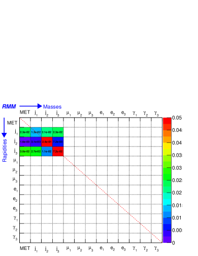
(a) RMM for hadronic decay of $t\bar{t}$

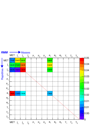
(b) RMM for semileptonic decay of $t\bar{t}$

Figure 1: Visualization of the T4N3 RMMs for two $t\bar{t}$ events: (a) an event where $t$($\bar{t}$) decay to six jets. (b) an event where one top quark decays to $\bar{b}W^{+}$ with $W^{+}\to e^{+}\nu_{e}$. The latter event activates the cell at the position (1,1) which contains the information on $E_{T}^{\mathrm{miss}}$ scaled by $1/\sqrt{s}$. The first row contains scaled transverse masses, $m_{T}(i)$. The red dashed line shows the diagonal elements with transverse energy and their imbalances. The upper-right part of this matrix contains $m(i,j)$, while the lower-left part contains rapidity differences, $h(i,j)$. The type of objects for each RMM cell is indicated.

In addition to the Standard Model processes, events with charged Higgs boson ($H^{+}$) process were generated using the diagram $bg\to H^{+}t$, which is an attractive exotic process Akeroyd et al. (2017) arising in models with two (or more) Higgs doublets. This process was also simulated with Pythia8 assuming a mass of 600 GeV for the $H^{+}$ boson, which decays to $W^{+}$ and $H$. In order make the identification of this process more challenging for our later discussion, we will consider $H$ decaying to two $b$-jets. In this case, the event signatures (and the RMM values) are rather similar to those from the $t\bar{t}$ production.

(a) Multi-jets QCD

(b) Higgs processes

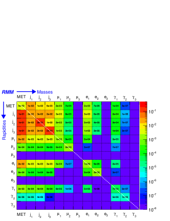
(c) Top ($t\bar{t}$) production

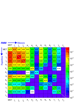
(d) $H^{+}t$ production

Figure 2: Visualization of the T4N3 RMMs for four different processes using 50,000 Monte Carlo events for each process (with all decay modes allowed for top quarks, vector bosons and $H$). In the case of $H^{+}$ decaying to $W^{+}$ and $H$, $H$ decays to $b-$jets. The cell position (1,1) contains the information with a missing transverse energy $E_{T}^{\mathrm{miss}}$ scaled by $1/\sqrt{s}$. The first row contains scaled transverse masses $m_{T}(i)$. The white dashed line shows the diagonal elements with transverse energy and their imbalances. The upper-right part of this matrix contains $m(i,j)$, while the lower-left part contains rapidity differences, $h(i,j)$.

The software and Monte Carlo settings were taken from the HepSim project Chekanov (2015). Stable particles with a lifetime larger than $3\cdot 10^{-10}$ seconds were considered, while neutrinos were excluded from consideration. The jets were reconstructed with the anti-$k_{T}$ algorithm Cacciari et al. (2008) as implemented in the FastJet package Cacciari et al. (2012) using a distance parameter of $R=0.6$. The minimum transverse energy of jets was $50$ GeV, and the pseudorapidity range was $|\eta|<3$. Muons, electrons and photons were reconstructed from the truth-level record, making sure that they are isolated from jets. The minimum transverse momentum of leptons and photons was 25 GeV. The missing transverse energy is recorded only if it is above 50 GeV.

For a better understanding the RMM formalism, Fig. 1 shows two events with $t\bar{t}$ from the Pythia8 generator. Fig. 1(a) shows an event where $t$ and $\bar{t}$ quarks decay to six jets, while Fig. 1(b) shows an event where one top quark decays to $\bar{b}W^{+}$ with $W^{+}\to e^{+}\nu_{e}$. The figures show rather distinct patterns for these two events. The six-jet event does not have leptons and $E_{T}^{\mathrm{miss}}$ (at the position (1,1)). Note that the simple T4N3 configuration used in this paper to illustrate the RMM concept is not appropriate for real-life cases since it cannot accommodate all reconstructed jets, nor $b-$jets. How to determine the RMM configuration will be explained at the end of Sect. V.

The RMMs matrices can also be used for visualizing groups with many events. Figure 2 shows the average values of T4N3 RMM cells for the Monte Carlo events described above. As in the case of single events, the figures show rather distinct patterns for these four processes. The QCD multijet events do not have large values of $E_{T}^{\mathrm{miss}}$ at the position (1,1), and there is no large rates of leptons and photons. The Higgs processes have an enhanced production of two photons and leptons, indicated with significant values at ($\gamma_{1},\gamma_{2}$), ($\mu_{1},\mu_{2}$) and ($e_{1},e_{2}$). If one considers ($\gamma_{1},\gamma_{2}$) cells only, the Higgs mass can be reconstructed from the $m(\gamma_{1},\gamma_{2})$ cells shown in Fig. 2(b), after multiplying their values by $\sqrt{s}$. The $t\bar{t}$ events have a large missing transverse energy at (1,1) and a significant jet activity. The largest similarity between RMMs was found for the $H^{+}$ and $t\bar{t}$ events shown in Figs. 2(c) and (d). If a single decay channel is considered for $H^{+}\to W^{+}H$, such as $H$ decaying to two photons, the RMM for $H^{+}$ will be significantly different from the other processes.

IV RMM for Neural Networks

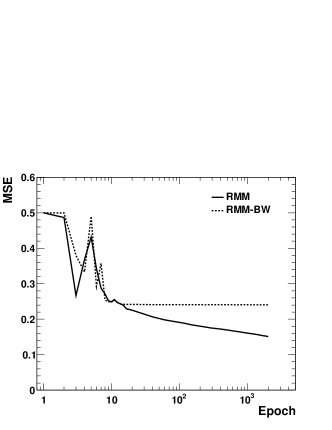
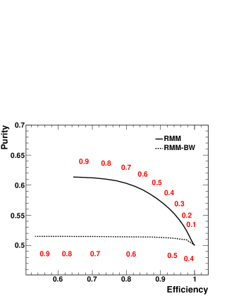
Figure 3: (a) MSE values versus epoch for the separation of $H^{+}$ from background $t\bar{t}$ events using the NN. The solid line shows the standard RMM, while the dashed line shows a version of the RMM where non-zero values are replaced by 1 (RMM-BW). A shallow backpropagation NN was used with 169 input nodes, 120 nodes in a single hidden layer, and one node in the output layer. 10,000 events of each category were used for the NN training. The training was terminated using a cross validation sample. Figure (b) shows the reconstruction efficiency of $H^{+}$ events versus the reconstruction purity for the standard RMM and RMM-BW. The values of the output node at fixed values of the efficiency are shown above (below) the curves. i

An identification of the Standard Model processes, such as multijet QCD, Higgs and $t\bar{t}$ does not represent any challenge for the NN classification, since even the visualized RMMs show different patterns for these processes. However, the separation of $H^{+}$ events from $t\bar{t}$ is more difficult due to the similarity of their RMMs. The main distinct feature of these two processes is the RMM cell values, i.e. the color patterns shown in Fig. 2, not the numbers of non-zero cells in events. Therefore, the $H^{+}$ and $t\bar{t}$ events were used to verify the classification capabilities of the RMM.

As simple test of the RMM concept for event classification using machine learning, we have created 10,000 RMMs for $H^{+}$ and $t\bar{t}$ events, which are then used as the input for a shallow backpropagation NN with the sigmoid activation function. The NN was implemented using the FANN package Nissen . No re-scaling of the input values was applied since the value range of $[0,1]$ is fixed by the definition of the RMM. The NN had 169 input nodes, which were mapped to a 1D array obtained from T4N3 RMM with a size of $13\times 13$. A single hidden layer had 120 nodes, while the output layer had a single node. During the NN training, the output node value was set to 0 for $t\bar{t}$ events and to 1 for $H^{+}$ events. This value corresponds to a probability that a given collision event belongs to the $H^{+}$ category. The NN was trained using 2,000 epochs. The training was terminated using an independent (”cross-validation”) sample with 10,000 RMMs. It was found that the MSE of the validation sample does not decrease with the number of epochs after 2,000 epochs.

To understand the performance of the NN, the default activation function was changed to a linear activation function in the FANN package Nissen . The number of nodes in the hidden layer was varied in the range (50-400). In addition, the number of hidden nodes was increased to two. No significant changes in the NN performance were found.

Figure 3(a) shows that the mean square error (MSE) of the NN based on the RMM decreases as a function of the epoch number (the solid line). This indicates a well-behaved NN training. A spike for small number of epochs is due the gradient-descent optimization applied to the sparse input data. In addition to the standard RMM, this figure shows a special case when all values of the RMM were set to 1 for cells with non-zero values (i.e. converting the RMMs to “black-and-white” images). Such 2D arrays, called RMM-BW, were constructed to check the sensitivity of the NN output to the amplitude of the cell values. According to Fig. 3(a), the NN with the RMM-BW inputs cannot effectively be trained, since the MSE values are independent of the epoch number. Therefore, for the given example, the number of cells containing zero values in the RMM (and thus the multiplicities of objects) is not an important factor for the NN training.

To verify the performance of the trained NN, a sample of RMMs was constructed from $t\bar{t}$ and $H^{+}$ events which were not used during the training procedure. Then the trained NN was applied for predicting the output node value. The success of the NN training was evaluated in terms of the purity of the reconstructed $H^{+}$ events as a function of the reconstructed efficiency. The efficiency of identification of $H^{+}$ events was defined as a fraction of the number of true $H^{+}$ events with the NN output above some value. This value can be varied between 0 and 1, with 1 being the most probable likelihood that the event belongs to $H^{+}$ process. We also calculated the purity of the reconstructed $H^{+}$ events as a ratio of the number of $H^{+}$ events that met a requirement on the NN output value, divided by the number of accepted events (irrespective of the origin of these events). Both the efficiency and purity depend on the value of the output node.

Figure 3(b) shows the performance of the NN event classifier in terms of the efficiency to identify the $H^{+}$ events versus the event purity for several requirements on the NN output value. For the used Monte Carlo event samples, the statistical uncertainties on the purity-efficiency curves are less than 3%.

According to this figure, the standard RMM can be used to identify $H^{+}$ events. The RMM-BW input for the NN fails for the event classification due to the lack of influential features.

V Event classification for searches

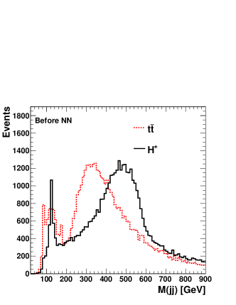
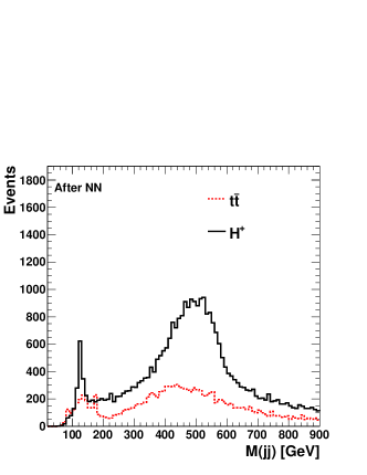
Figure 4: Invariant masses of two leading in $E_{T}$ jets for $t\bar{t}$ and $H^{+}$ event categories before (a) and after (b) applying the NN based on RMM inputs and requiring the NN output values above 0.5. The NN was trained after disabling the cells that carry information on the masses of two leading jets. The number of events for each event category ($t\bar{t}$ and $H^{+}$) is 50,000. The dijet masses were reconstructed from the RMM cell (3,2). Statistical uncertainties for each histogram are given by the square root of the number of entries in each bin (not shown).

The RMMs can project complex collision events into to a fixed-size phase space, such that the mapping of the RMM cells to the NN with a fixed number of the input nodes is unique, independent of how many objects are produced. A well-defined input space is the requirement for many machine learning algorithms. At the same time, the RMM covers almost every aspect of particle/jet production in terms of major (weakly correlated) kinematic variables. Therefore, studies of the most influential variables used for classification of events can be reduced or even avoided. However, in some situations, in order to reduce biases that can distort background distributions towards signal features, RMM cells with variables to be used for physics measurements need to be identified and disregarded during machine learning.

Let us consider a simple example. We will separate the $H^{+}$ events (“signal”) from $t\bar{t}$ (“background”) using the NN based on the RMMs. As a measure of our success in the event classification, we will use the invariant masses of two leading in $E_{T}$ jets which correspond to the cell position (3,2). This variable will also be used to perform physics studies, such as the measurement of the $H^{+}$ mass. The distribution of this variable should (preferably) be unbiased by the NN training. Therefore, we will disable $e_{T}(i)$ and $m(i,j)$ inputs at the RMM positions (2,2) and (3,2) during the NN training.

Figure 4(a) shows the dijet mass distribution reconstructed from the RMM after summing up the cell values at the position (3,2) over all events, and scaling the sum by $\sqrt{s}$. We use 50,000 events for each process category, i.e. for the signal ($H^{+}$) and background events ($t\bar{t}$). A sharp peak observed at 125 GeV is due to the decay $H\to b\bar{b}$, when each $b$-quark forms a jet. A broad peak near $500$ GeV is due to the decays of $H^{+}$ to $W(\to q\bar{q})$ and $H(\to b\bar{b})$, when the decay products of $W$ and $H$ are merged by the jet algorithm to form two jets. The peak position of the latter is shifted from the generated $H^{+}$ mass of 600 GeV. This is due to the fact that the jet algorithm has a size of 0.6, which is not large enough to collect all hadronic activity from boosted $W$ and $H$. The $t\bar{t}$ events generated as explained above represent a background which masks the $H^{+}$ signal. Note that, in real-life scenarios, the rate of the background $t\bar{t}$ events is significantly larger than that given in this toy example.

The NN with the two disabled input links described above was trained using 10,000 events with $t\bar{t}$ and $H^{+}$. The trained NN was applied to classify the event sample with 50,000 events per each event category. We accept $H^{+}$ events when the value of the output node is above 0.5. After applying the NN selection, one can successfully reduce the $t\bar{t}$ background, as shown in Fig. 4(b). The background distribution is somewhat shifted towards the signal peak, indicating that some residual effect from the NN training is still present. But this bias cannot change our main conclusion that the signal can reliably be identified. The NN selection decreases the background at the 500 GeV mass region by a factor 3, while the $H^{+}$ signal rate is only reduced by $30\%$. Note that the background contribution to the $H^{+}$ events depends on the realistic event rates of the $t\bar{t}$ and $H^{+}$ processes, which are not considered in this example.

A comment on evaluation of systematic uncertainties when using the RMM should follow. As in the case of the usual cut-and-reject methods, the RMM matrices should be recalculated using different conditions for all reconstructed objects. In the case of calculations of statistical limits, the histograms obtained after applying the RMM selections should be included in dedicated programs for limit calculations.

We believe that the event classification capabilities of this approach can significantly be increased by considering RMMs with more than three jets, leptons with different charges, $b$-jets, reconstructed $\tau$ leptons, or using multi-dimensional matrices with three or more particle correlations. To improve classification, a care should be taken to avoid a “saturation” effect when multiplicities of particles/jets are larger than the chosen $N_{i}$ that define the RMM size, otherwise the loss of useful information may prevent an effective usage of the RMM. We used $N_{i}=3$ in the simple example described above for better explanation and visualization of this method. This is not a sufficiently large number for the chosen transverse momentum cut in order to accommodate events with a large number of jets. Note that larger values of $N_{i}$ do not increase dramatically the sizes of the files used for storing sparse matrices since only non-zero values of cells (and their indices) are kept. A more sophisticated event classification and comparisons with alternative machine learning techniques are beyond the computational resources dedicated to this paper. Other examples of event classifications using the RMM approach were considered in Ref. Chekanov (2018).

VI Conclusion

We propose a method to transform events from colliding experiments to the language widely used by machine learning algorithms, i.e. fixed-size sparse matrices. In addition, the RMM transformation can be viewed as an effective mapping of complex collision data to pixelated representation useful for visual study. The method does not exclude the use of different types of neural network (deep or recurrent) or other machine learning techniques.

By construction, groups of RMMs cells that belong to certain types of objects are connected by proximity due to a well-defined hierarchy of the kinematic variables. Therefore, the usage of the RMM in particle physics may leverage widely used algorithms developed for image identification that exploit local connectivity of pixels (cells).

Our tests indicate that the proposed approach of imaging collision data for event classification can be useful for preparing a feature space for machine learning. The RMM method is sufficiently general and, typically, does not require detailed studies of influential variables sensitive to background events. But care should be taken to avoid using NN inputs that may bias the shapes of observables which will be used later in searches for new physics. The C++ library that transforms the event records to the RMM is available Chekanov .

Appendices

Appendix A Correlation coefficients of the RMM

Table 1: RMM cells with the values of the Pearson correlation coefficients ($\rho$) larger than 15%. The coefficients were calculated from the Pythia8 Monte Carlo simulations described in Sect. III. The first column shows the correlation coefficients, the second column shows the position of the first cell, and the third column shows the position of the second cell. In the RMM notation, the largest correlation (92%) is observed for the transverse masses calculated using leading and sub-leading jets.

$\rho$	(r1,c1)	(r2, c2)
0.92	2,1	3,1
0.87	5,2	5,5
0.87	1,1	2,1
0.83	1,1	3,1
0.82	3,1	4,1
0.81	5,2	5,3
0.80	6,2	6,3
0.80	6,1	6,2
0.79	6,2	6,5
0.79	5,3	5,5
0.79	4,6	6,4
0.79	2,2	3,2
0.78	2,1	4,1
0.77	2,6	6,2
0.76	6,1	6,5
0.76	3,6	6,3
0.75	5,3	5,4
0.74	6,3	6,5
0.74	5,1	5,2
0.74	4,5	5,4
0.74	1,1	4,1
0.72	6,5	6,6
0.72	5,6	6,5
0.71	5,2	5,4
0.70	3,5	5,3
0.69	5,1	5,5
0.69	1,6	6,1
0.68	6,3	6,4
0.68	6,1	6,3
0.67	5,4	5,5
0.67	3,4	4,3
0.66	6,1	6,6
0.65	5,1	5,3
0.65	1,6	6,2
0.63	6,2	6,6
0.63	5,6	6,2
0.62	2,5	5,2
0.62	1,6	2,6
0.61	3,6	6,4
0.60	4,2	4,3
0.60	3,6	4,6
0.59	2,6	5,6
0.59	2,4	4,2
0.58	6,2	6,4
0.58	2,2	4,2
0.57	3,2	4,2
0.57	2,6	6,1
0.55	5,6	6,3
0.54	6,3	6,6
0.54	5,1	5,4
0.54	3,6	6,2
0.53	5,6	6,1

$\rho$	(r1,c1)	(r2, c2)
0.53	1,6	6,5
0.53	1,6	6,3
0.53	1,6	5,6
0.52	1,5	2,5
0.51	2,6	6,5
0.51	2,6	6,3
0.50	6,4	6,5
0.49	3,6	6,5
0.49	3,2	4,3
0.48	4,6	6,3
0.47	3,6	5,6
0.47	1,6	3,6
0.47	1,5	3,5
0.46	1,5	5,3
0.46	1,5	5,2
0.46	1,5	5,1
0.45	3,6	6,1
0.45	2,5	5,3
0.45	2,5	3,5
0.45	1,5	4,5
0.44	6,1	6,4
0.44	3,5	5,4
0.44	3,5	5,2
0.44	2,6	3,6
0.43	5,6	6,6
0.43	4,5	5,3
0.43	2,6	6,6
0.43	1,6	6,6
0.43	1,5	5,4
0.42	5,6	6,4
0.42	3,5	4,5
0.42	3,2	4,4
0.41	2,3	3,2
0.40	2,5	5,4
0.40	2,5	4,5
0.40	2,2	4,3
0.40	1,4	2,4
0.39	4,5	5,2
0.38	2,5	5,1
0.37	1,6	6,4
0.37	1,6	4,6
0.37	1,4	3,4
0.37	1,1	5,1
0.36	6,4	6,6
0.36	3,5	5,1
0.35	3,6	6,6
0.34	3,5	5,5
0.34	2,2	4,4
0.34	1,5	5,5
0.33	4,6	6,2
0.33	2,4	3,4
0.32	2,6	6,4

$\rho$	(r1,c1)	(r2, c2)
0.29	4,5	5,5
0.29	3,1	5,1
0.29	2,1	2,2
0.29	1,4	4,3
0.29	1,4	4,2
0.28	4,6	6,1
0.28	2,1	3,3
0.27	4,6	6,5
0.27	4,6	5,6
0.27	2,4	4,3
0.26	4,1	4,3
0.26	2,3	3,4
0.25	2,2	3,3
0.25	1,3	3,4
0.25	1,2	2,3
0.24	4,3	4,4
0.24	4,2	4,4
0.24	3,4	4,2
0.24	1,1	3,3
0.23	4,1	5,1
0.23	3,3	4,4
0.23	2,2	3,1
0.22	5,5	6,6
0.22	4,1	4,2
0.22	2,3	2,4
0.22	1,2	2,4
0.21	5,5	6,5
0.21	5,1	6,1
0.21	4,6	6,6
0.21	2,1	5,2
0.20	4,1	5,4
0.18	5,1	6,6
0.18	3,1	5,3
0.18	1,4	4,1
0.17	5,5	6,2
0.17	5,5	6,1
0.17	5,1	6,5
0.17	5,1	6,2
0.17	2,6	4,6
0.17	1,1	5,2
0.16	3,3	4,3
0.16	3,1	3,3
0.16	3,1	3,2
0.16	2,2	4,1
0.16	2,1	5,3
0.15	5,5	6,3
0.15	5,2	6,5
0.15	5,2	6,2
0.15	3,4	4,1
0.15	3,1	5,2
0.15	1,4	4,4

References

- Voss (2015) H. Voss, Journal of Physics: Conference Series 608, 012058 (2015).
- Bishop (2006) C. M. Bishop, Pattern Recognition and Machine Learning (Springer, 2006).
- Guest et al. (2018) D. Guest, K. Cranmer, and D. Whiteson, Ann. Rev. Nucl. Part. Sci. 68, 161 (2018), arXiv:1806.11484 [hep-ex] .
- Chekanov and Morgunov (2003) S. V. Chekanov and V. L. Morgunov, Phys. Rev. D67, 074011 (2003), arXiv:hep-ex/0301014 [hep-ex] .
- Santos et al. (2017) R. Santos et al., JINST 12, P04014 (2017), arXiv:1610.03088 [hep-ex] .
- Cogan et al. (2015) J. Cogan et al., Journal of High Energy Physics 2015, 118 (2015).
- Tovey (2008) D. R. Tovey, JHEP 04, 034 (2008), arXiv:0802.2879 [hep-ph] .
- Boveia and Doglioni (2018) A. Boveia and C. Doglioni, Ann. Rev. Nucl. Part. Sci. 68, 429 (2018), arXiv:1810.12238 [hep-ex] .
- Belyaev et al. (2017) N. Belyaev, R. Konoplich, and K. Prokofiev, Journal of Physics: Conference Series 934, 012030 (2017).
- The CMS Collaboration (2011) The CMS Collaboration, Phys. Rev. C 84, 024906 (2011), arXiv:1102.1957 [nucl-ex] .
- The ATLAS Collaboration (2017) The ATLAS Collaboration, Phys. Rev. D96, 052004 (2017), arXiv:1703.09127 [hep-ex] .
- The CMS Collaboration (2012) The CMS Collaboration, Eur. Phys. J. C72, 2216 (2012), arXiv:1204.0696 [hep-ex] .
- Sjostrand et al. (2006) T. Sjostrand, S. Mrenna, and P. Z. Skands, JHEP 05, 026 (2006), arXiv:hep-ph/0603175 .
- Sjostrand et al. (2008) T. Sjostrand, S. Mrenna, and P. Z. Skands, Comput. Phys. Commun. 178, 852 (2008), arXiv:0710.3820 [hep-ph] .
- Ball et al. (2013) R. D. Ball et al., Nucl. Phys. B867, 244 (2013), arXiv:1207.1303 [hep-ph] .
- Ball et al. (2015) R. D. Ball et al. (NNPDF), JHEP 04, 040 (2015), arXiv:1410.8849 [hep-ph] .
- Buckley et al. (2015) A. Buckley et al., Eur. Phys. J. C 75, 132 (2015), arXiv:1412.7420 [hep-ph] .
- Akeroyd et al. (2017) A. G. Akeroyd et al., Eur. Phys. J. C 77, 276 (2017), arXiv:1607.01320 [hep-ph] .
- Chekanov (2015) S. V. Chekanov, Adv. High Energy Phys. 2015, 136093 (2015), arXiv:1403.1886 [hep-ph] .
- Cacciari et al. (2008) M. Cacciari, G. P. Salam, and G. Soyez, JHEP 04, 063 (2008), arXiv:0802.1189 [hep-ph] .
- Cacciari et al. (2012) M. Cacciari, G. P. Salam, and G. Soyez, Eur. Phys. J. C 72, 1896 (2012), arXiv:1111.6097 [hep-ph] .
- (22) S. Nissen, “FANN. Fast Artificial Neural Network Library,” Web page. (accessed on Feb. 1st, 2019), http://leenissen.dk/fann/wp/.
- Chekanov (2018) S. V. Chekanov, “Machine learning using rapidity-mass matrices for event classification problems in HEP,” Preprint ANL-HEP-147750 (2018), arXiv:1810.06669 [hep-ph] .
- (24) S. Chekanov, “Map2RMM library,” Web page. (accessed on Feb. 1st, 2019), https://atlaswww.hep.anl.gov/asc/map2rmm/.