High-Fidelity Modeling of Detector Lag and Gantry Motion in CT Reconstruction

Abstract

Detector lag and gantry motion during x-ray exposure and integration both result in azimuthal blurring in CT reconstructions. These effects can degrade image quality both for high-resolution features as well as low-contrast details. In this work we consider a forward model for model-based iterative reconstruction (MBIR) that is sufficiently general to accommodate both of these physical effects. We integrate this forward model in a penalized, weighted, nonlinear least-square style objective function for joint reconstruction and correction of these blur effects. We show that modeling detector lag can reduce/remove the characteristic lag artifacts in head imaging in both a simulation study and physical experiments. Similarly, we show that azimuthal blur ordinarily introduced by gantry motion can be mitigated with proper reconstruction models. In particular, we find the largest image quality improvement at the periphery of the field-of-view where gantry motion artifacts are most pronounced. These experiments illustrate the generality of the underlying forward model, suggesting the potential application in modeling a number of physical effects that are traditionally ignored or mitigated through pre-corrections to measurement data.

I INTRODUCTION

The need for high-resolution, quantitatively accurate CT reconstructions has increased with the rise of application-specific systems. For example, Cone-Beam CT (CBCT) mammography [1] and extremities systems [2] require high resolution to detect microcalcifications and visualize fine trabecular structure, respectively. Point-of-care CBCT head imaging [3] similarly requires highly accurate reconstruction of relative attenuation values to detect low contrast bleeds. Such dedicated imaging systems often use flat-panel detectors, which are selected for their high-resolution capability and ease of integration into compact systems. However, a number of physical effects including scintillator blur and detector lag can degrade measurement data, challenging the above applications. Similar examples of hardware limitations challenging particular applications can be found in traditional Multi-Detector CT (MDCT). For example, cardiac and emergency room scanning place high demands on lowering the scan time. The high rotation rates in such applications can result in significant blurring effects due to gantry motion during the integration time of the detector.

Previous work has suggested that such hardware limitations can be compensated through explicit modeling and incorporation into a Model-Based Iterative Reconstruction (MBIR) algorithm. In particular, we have found that scintillator blur and focal-spot blur in flat-panel systems can be modeled for potential resolution recovery [4]. The forward model used in that work is very general and permits incorporation of a wide range of physical effects. In this work we adopt the same mathematical form for the underlying forward model and apply MBIR to detector lag and gantry motion.

Detector lag results from the detector trapping and later releasing charge, causing a fraction of the signal from previously acquired projections to be added (temporally blurred) into subsequent projections [5], [6]. Detector lag effects are usually low contrast and extend across large areas of the reconstruction, originating near high contrast objects. A classic example of lag artifacts are the low contrast trails arcing off the skull into the brain in flat-panel-based head imaging. Traditionally, detector lag corrections are applied through preprocessing the measurements prior to reconstruction [7, 8]. To our knowledge, this work is the first attempt to correct for lag within the forward model of an MBIR approach.

Gantry motion blur shares some similarity with lag in that there is an effective blurring over angle. However, this blur occurs within a single measurement - effectively integrating an arc of projection images based on how far the source and detector have rotated during an integration period. Such blur exhibits as an azimuthal smearing of the CT volume and is most pronounced toward the edge of the field of view. Gantry motion effects have been addressed in hardware (e.g., collecting data with a step-and-shoot protocol or more complicated methods [9]) and in software (e.g., incorporating a blur model into a linearized forward model for MBIR [10]).

In this paper, we introduce specific models of detector lag and gantry motion, and integrate those models into the general form in [4]. Simulation studies are conducted for both blur scenarios. Image reconstructions are performed using both traditional (unmodeled blur) and the proposed high-fidelity models, and the resulting images are compared. Preliminary physical-experiment results using a head phantom and a CBCT test bench are also shown to illustrate application in a real system.

II METHODS

Both detector lag and gantry motion blur scenarios can use the same general forward model presented in [4]:

$$\bar{\bm{y}}=\bm{\mathrm{B}}\exp\left(-\bm{\mathrm{A}}\bm{\mu}\right)$$ (1a)

$$y\sim\operatorname{\mathcal{N}}\left(\bar{\bm{y}},\bm{\mathrm{K}}\right)$$ (1b)

where $\bm{\mathrm{B}}$, $\bm{\mathrm{A}}$, and $\bm{\mathrm{K}}$ are matrices, $\bm{\mu}$ is a vector of attenuation values, and $\bm{y}$ is a vector of measurements. The corresponding penalized likelihood objective function is

$$\left\|\left(\bm{y}-\bm{\mathrm{B}}\exp\left(-\bm{\mathrm{A}}\bm{\mu}\right)\right)\right\|^{2}_{\bm{\mathrm{K}}^{-1}}+\beta\operatorname{R}(\bm{\mu})$$ (2)

where R is a penalty function and $\beta$ is the penalty strength. The $\bm{\mu}$ that minimizes (2) is the reconstruction. A traditional forward model has $\bm{\mathrm{A}}$ as the system matrix, $\bm{\mathrm{B}}$ as a diagonal matrix which scales measurements by a gain factor (e.g., photon flux, etc.), and $\bm{\mathrm{K}}$ as a diagonal matrix of measurement variances. However, the reconstruction method in [4] which minimizes the objective function (2) makes few assumptions about these matrices, allowing the forward model (1b) to incorporate many physical properties. This reconstruction method may utilize ordered subsets and Nesterov momentum acceleration [11, 12].

II-A Detector lag

Detector lag may be modeled as a convolution blur where the blur kernel is a sum of exponentials [8]:

$$h[k]=\begin{cases}b_{0}\delta[k]+\sum_{i=1}^{3}b_{i}\exp\left(-ka_{i}\right)&\text{if }0\leq k<K\\ 0&\text{otherwise}\end{cases}.$$ (3)

The $K$ parameter in (3) determines the length of the blur kernel (i.e., the number of nonzero terms). This convolution is incorporated into $\bm{\mathrm{B}}$ in (1a). Specifically, each row of $\bm{\mathrm{B}}$ weights and combines a series of unblurred measurement data to form a measurment with lag. Physical blur kernel parameters for our test bench system were estimated from the falling edge of a bare-beam scan [8]. The estimated parameters used throughout this work are shown in Table II-A. Because $\bm{\mathrm{B}}$ is no longer block diagonal with regards to projection number (i.e., $\bm{\mathrm{B}}$ blurs among projections), we cannot trivially apply ordered subsets to speed convergence [13].

TABLE I: Blur kernel parameters

	0	1	2	3
a	—	0.998	0.0991	0.0152
b	0.965	0.0165	0.000572	4.51e-05

A simulation study was conducted with an ellipsoidal “head” phantom of fat surrounded by bone. Data were generated from a phantom with $0.25\text{\times}0.25\text{\,}\mathrm{mm}$ voxels on a system with $580.0\text{\,}\mathrm{mm}$ Source-Isocenter Distance (SID) and $800\text{\,}\mathrm{mm}$ Source-Detector Distance (SDD). Data were projected onto a detector with $0.278\text{\,}\mathrm{mm}$ pixels with $0.5\text{\times}{10}^{5}\text{\,}\mathrm{photons}\text{\,}{\mathrm{pixel}}^{-1}$ over $360\mathrm{°}$ in $1\mathrm{°}$ increments. Poisson noise was added and data were binned by a factor of two, resulting in $0.556\text{\,}\mathrm{mm}$ pixels with ${10}^{6}\text{\,}\mathrm{photons}\text{\,}{\mathrm{pixel}}^{-1}$. We then blurred the data by the calculated blur kernel with a length of $K=359$ and added readout noise ($\sigma_{ro}=$ $7.12\text{\,}\mathrm{photons}$). Blurring the data after adding Poisson noise correlates the noise as in real systems [6].

Data were reconstructed with $0.5\text{\times}0.5\text{\,}\mathrm{mm}$ voxels, a quadratic regularizer, and the separable footprints projector [14]. Two reconstruction methods were used: identity blur modeling (i.e., no blur modeling) and detector lag blur modeling (with a kernel length of $K=101$). In this work we assume uncorrelated noise for simplicity, specifically

$$\bm{\mathrm{K}}=\operatorname{D}\{\bm{y}\}+\sigma_{ro}^{2},$$ (4)

where $\operatorname{D}\{\cdot\}$ is a diagonal matrix with its argument on the diagonal). We used $5000$ iterations and Nesterov acceleration. Reconstructions were noise matched by varying $\beta$ and taking the standard deviation of the attenuation values in the center of the image.

Additionally, we scanned a physical head phantom on a CBCT test bench with parameters similar to those in the simulation study, except projection data were acquired in half angle increments. In order to focus on only detector lag in this preliminary study, we corrected the data for beam hardening due to water, scatter, and glare, as described in [15]. Data were reconstructed with $0.5\text{\times}0.5\text{\times}0.5\text{\,}\mathrm{mm}$ voxels using the same blur models as the simulation study (the blur model used a lag kernel length of $K=201$). Nesterov acceleration was used with $4000$ iterations. We used a quadratic regularizer, and the same regularization strength for both reconstructions.

II-B Gantry motion

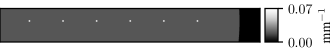
Figure 1: A portion of the digital phantom for motion blur studies. The left most circle in this figure is at the center of the phantom. The circles are separated by $20\text{\,}\mathrm{mm}$.

Gantry motion blur is the result of a continuous integration over angle, and may be modeled as

$$\bar{\bm{y}}_{i}=\bm{\mathrm{B}}_{2}\int_{\psi=\theta_{i}-\Delta\theta/2}^{\theta_{i}+\Delta\theta/2}\exp(-\bm{\mathrm{A}}_{\psi}\bm{\mu})\mathrm{d}\psi$$ (5)

where $\bar{\bm{y}}_{i}$ is the mean measurement vector at projection $i$ and gantry angle $\theta_{i}$, $\Delta\theta$ is the angular distance over which data is collected for projection $i$, and $\bm{\mathrm{A}}_{\psi}$ is the projection matrix at angle $\psi$. A discrete approximation is achieved by oversampling in projection angle and summing the results to obtain the measurement sampling:

$$\bar{\bm{y}}_{i}=\bm{\mathrm{B}}_{2}J^{-1}\sum_{j=0}^{J}\exp\left(-\bm{\mathrm{A}}_{\psi}\bm{\mu}\right)$$ (6)

$$\psi(j)=\theta_{i}+\Delta\theta\left(j/J-1/2\right)$$ (7)

where $J$ is the angular oversampling factor. $\bm{\mathrm{B}}$ from (1b) contains $\bm{\mathrm{B}}_{2}$ and the summation term in (6), and $\bm{\mathrm{A}}$ contains all the $\bm{\mathrm{A}}_{\psi}$ used in (6). For example, if the measurement data contains $360$ projections and $J$ is 3, then $\bm{\mathrm{A}}$ results in $1080$ projections, and every three consecutive projections are summed together as part of $\bm{\mathrm{B}}$.

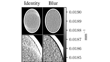
Figure 2: Simulation phantom reconstructions with the identity model (left) and the detector lag model (right). The second row of images shows a smaller portion of the phantom for better visualization.

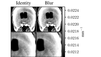
Figure 3: Head phantom bench reconstructions with the identity model (left) and the detector lag model (right). The second row shows a smaller portion of the phantom to better visualize the detector lag effect.

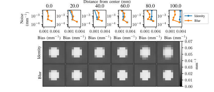
Figure 4: Bias/noise curves (top) and reconstructions (bottom) for each ROI in Fig. 1. Each column corresponds to a distance from the center of rotation. The top row reconstructions use the identity model and the bottom row reconstructions use the gantry motion blur model.

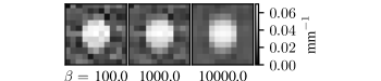
Figure 5: Quadratic penalty reconstructions of the $100\text{\,}\mathrm{mm}$ ROI with blur modeling.

A circular simulation phantom with a diameter of $25\text{\,}\mathrm{cm}$ and multiple round ROIs at different distances from the center of rotation was used to evaluate the proposed algorithm. A subset of this phantom is shown in Fig. 1. A continuous motion system was simulated with $500\text{\,}\mathrm{mm}$ SID, $1000\text{\,}\mathrm{mm}$ SDD, and 1000 projections per rotation. This geometry was chosen to approximate high-resolution MDCT systems. Data were generated from a phantom with $0.1\text{\times}0.1\text{\,}\mathrm{mm}$ voxels and a detector with $0.125\text{\,}\mathrm{mm}$ pixel pitch. We projected at $51\,000$ equally spaced angles over a $360\mathrm{°}$ rotation. Poisson noise was added prior to binning to $1000$ projections and spatially binning to $0.25\text{\,}\mathrm{mm}$ pixels. The photon flux after binning was ${10}^{5}\text{\,}\mathrm{photons}\text{\,}{\mathrm{pixel}}^{-1}$. Finally, readout noise was added to the data ($\sigma_{ro}=$ $7.12\text{\,}\mathrm{photons}$).

Data were reconstructed with $0.2\text{\times}0.2\text{\,}\mathrm{mm}$ voxels. We used two blur models: an identity blur model (no blur, $\bm{\mathrm{A}}$ produces $1000$ projections), and a gantry motion blur model with an angular oversampling factor of $J=5$ ($\bm{\mathrm{A}}$ produces 5000 projections). We used an uncorrelated noise model (4), the Huber penalty ($\delta=$ ${10}^{-3}$) [16], and the separable footprints projector [14]. Nesterov acceleration was used with $1000$ iterations and $10$ subsets. Bias/noise measurements were calculated for each ROI. Bias was the Root Mean Squared Error (RMSE) between a noiseless reconstruction and truth at the ROI, and noise was the RMSE between a noisy reconstruction and a noiseless reconstruction in a nearby region. Bias and noise were calculated for multiple penalty strengths to obtain a bias/noise curve for each method. Data were also reconstructed with a quadratic penalty and $J=5$ to compare this penalty to the Huber penalty.

III RESULTS

III-A Detector lag

The detector lag digital phantom reconstructions are shown in Fig. 2. The reconstructions are approximately noise matched — $7.96\text{\times}{10}^{-05}\text{\,}{\mathrm{mm}}^{-1}$ (identity) and $7.91\text{\times}{10}^{-05}\text{\,}{\mathrm{mm}}^{-1}$ (blur). When no blur model is used, detector lag causes a bright trail atrifact arcing off the skull and into the interior of the head. When blur modeling is used, this effect is eliminated. When lag modeling was applied to bench data, the bright trail off the skull was dramatically reduced (Fig. 3). The fact that the trail was not completely removed may be due to an insufficient number of iterations (non-converged estimate) or an inaccurate estimate of the lag blur kernel.

III-B Gantry motion

Gantry motion results are summarized in Fig. 4. The bias/noise tradeoff is shown for each ROI at varying distances from the center of rotation. The identity model suffers from increased bias at large distances from the center of rotation, while the blur model bias is relatively unchanged (suggesting a recovery of spatial resolution). The identity model appears to outperform the blur model at $20\text{\,}\mathrm{mm}60\text{\,}\mathrm{mm}$ from the center of rotation, although the difference is small. These results are confirmed in the reconstructions in Fig. 4. These reconstructions were approximately noise matched at the ROI furthest from the center of rotation by altering penalty strength (noise is $3.790\text{\times}{10}^{-04}\text{\,}\mathrm{mm}$ for the identity model and $3.407\text{\times}{10}^{-04}\text{\,}\mathrm{mm}$ for the blur model). The circles in the identity model reconstruction get blurrier along the direction of rotation as distance from the center increases. However, with the blur model the circles are accurately reconstructed. Additionally, the blur model’s bias improvement in the $20\text{\,}\mathrm{mm}60\text{\,}\mathrm{mm}$ range is difficult to visualize.

Fig. 5 shows the $100\text{\,}\mathrm{mm}$ ROI reconstructed with the blur model and the quadratic penalty at three different penalty strengths. With this penalty the blur model is unable to deblur the circle without a substantial increase in noise.

IV DISCUSSION

We have shown that the general reconstruction method presented previously [4] is capable of reducing effects due to detector lag and gantry motion blur. The methods presented here could trivially be extended to model detector lag with other forms (i.e., not sum of exponentials) or more complicated forms of gantry motion (e.g., when data acquisition only occurs during a fraction of the rotation). Additionally, these models may be combined with each other or other forms of blur, such as focal spot blur and scintillator blur, to further improve image quality.

A major limitation of modeling detector lag is the inability to use ordered subsets to speed convergence. In practice, one may initialize with a reconstruction without a lag model and with ordered subsets to get a relatively accurate estimate, and then reconstruct with the lag model for a handful of iterations. Additionally, a more accurate initialization may be obtained by lag correcting the projection data prior to simple MBIR (i.e., without lag modeling), and then the final reconstruction obtained with a few iterations with the full lag model and the original, uncorrected measurement data.

While this work is still preliminary, we note that the edge preserving Huber penalty plays an important role in the gantry motion reconstructions. We believe the quadratic penalty’s tendency to enforce smooth edges prevents the fidelity term from deblurring the gantry motion effects. In contrast, the Huber penalty doesn’t penalize sharp edges to the same degree, and allows the fidelity term to deblur the image. Ongoing work will further explore these issues by analyzing different penalties (e.g., sweeping the $\delta$ parameter) and using more complicated image quality targets.

High-fidelity system modeling with MBIR can improve image quality by overcoming hardware limitations such as detector lag and gantry motion. However, application specific systems may have different limitations and constraints. The forward model and MBIR algorithm used in this work are sufficiently general to accommodate many physical effects, and may therefore be used to improve image quality and quantitative accuracy in a wide range of clinical scenarios.

V ACKNOWLEDGMENTS

This work was supported in part by NIH grant F31 EB023783. The bench data used in this work was acquired with support of an academic-industry partnership with Carestream (Rochester, NY). The authors would like to thank Ali Uneri and Yoshi Otake for GPU software contributions.

References

- [1] J. M. Boone and K. K. Lindfors, “Breast CT: Potential for breast cancer screening and diagnosis.” Future oncology (London, England), vol. 2, no. 3, pp. 351–356, 2006.
- [2] E. Marinetto, M. Brehler, A. Sisniega, Q. Cao, J. W. Stayman, J. Yorkston, J. H. Siewerdsen, and W. Zbijewski, “Quantification of bone microarchitecture in ultrahigh resolution extremities conebeam CT with a CMOS detector and compensation of patient motion,” in Computer Assisted Radiology 30th International Congress and Exhibition, Heidelberg, Germany, Jun. 2016, pp. S20–S21.
- [3] J. Xu, A. Sisniega, W. Zbijewski, H. Dang, J. W. Stayman, M. Mow, X. Wang, D. H. Foos, V. E. Koliatsos, N. Aygun, and J. H. Siewerdsen, “Technical assessment of a prototype cone-beam CT system for imaging of acute intracranial hemorrhage,” Medical Physics, vol. 43, no. 10, pp. 5745–5757, Oct. 2016.
- [4] S. Tilley, M. Jacobson, Q. Cao, M. Brehler, A. Sisniega, W. Zbijewski, and J. W. Stayman, “Penalized-Likelihood Reconstruction with High-Fidelity Measurement Models for High-Resolution Cone-Beam Imaging,” IEEE Transactions on Medical Imaging, vol. PP, no. 99, pp. 1–1, 2017.
- [5] L. E. Antonuk, Y. El-Mohri, J. H. Siewerdsen, J. Yorkston, W. Huang, V. E. Scarpine, and R. A. Street, “Empirical investigation of the signal performance of a high-resolution, indirect detection, active matrix flat-panel imager (AMFPI) for fluoroscopic and radiographic operation,” Medical Physics, vol. 24, no. 1, pp. 51–70, Jan. 1997.
- [6] J. H. Siewerdsen, L. E. Antonuk, Y. el-Mohri, J. Yorkston, W. Huang, J. M. Boudry, and I. A. Cunningham, “Empirical and theoretical investigation of the noise performance of indirect detection, active matrix flat-panel imagers (AMFPIs) for diagnostic radiology,” Medical Physics, vol. 24, no. 1, pp. 71–89, Jan. 1997.
- [7] J. Starman, J. Star-Lack, G. Virshup, E. Shapiro, and R. Fahrig, “A nonlinear lag correction algorithm for a-Si flat-panel x-ray detectors,” Medical Physics, vol. 39, no. 10, pp. 6035–6047, Oct. 2012.
- [8] ——, “Investigation into the optimal linear time-invariant lag correction for radar artifact removal,” Medical Physics, vol. 38, no. 5, pp. 2398–2411, May 2011.
- [9] T. Nowak, M. Hupfer, F. Althoff, R. Brauweiler, F. Eisa, C. Steiding, and W. A. Kalender, “Time-delayed summation as a means of improving resolution on fast rotating computed tomography systems,” Medical Physics, vol. 39, no. 4, pp. 2249–2260, Apr. 2012.
- [10] J. Cant, W. J. Palenstijn, G. Behiels, and J. Sijbers, “Modeling blurring effects due to continuous gantry rotation: Application to region of interest tomography,” Medical Physics, vol. 42, no. 5, pp. 2709–2717, May 2015.
- [11] Y. Nesterov, “Smooth minimization of non-smooth functions,” Mathematical Programming Journal, Series A, vol. 103, pp. 127–152, 2005.
- [12] D. Kim, S. Ramani, and J. A. Fessler, “Combining Ordered Subsets and Momentum for Accelerated X-Ray CT Image Reconstruction,” IEEE Transactions on Medical Imaging, vol. 34, no. 1, pp. 167–178, 2015.
- [13] J. Nuyts, B. De Man, J. A. Fessler, W. Zbijewski, and F. J. Beekman, “Modelling the physics in iterative reconstruction for transmission computed tomography,” Physics in medicine and biology, vol. 58, no. 12, pp. R63–R96, Jun. 2013.
- [14] Y. Long, J. A. Fessler, and J. M. Balter, “3D forward and back-projection for X-ray CT using separable footprints.” IEEE Transactions on Medical Imaging, vol. 29, no. 11, pp. 1839–50, Nov. 2010.
- [15] A. Sisniega, W. Zbijewski, J. Xu, H. Dang, J. W. Stayman, J. Yorkston, N. Aygun, V. Koliatsos, and J. H. Siewerdsen, “High-fidelity artifact correction for cone-beam CT imaging of the brain,” Physics in Medicine and Biology, vol. 60, no. 4, p. 1415, 2015.
- [16] P. J. Huber, Robust Statistics. New York: Wiley, 1981.