A gapped $\mathrm{SU}(3)$ spin liquid with $\mathbb{Z}_{3}$ topological order

Abstract

We construct a topological spin liquid (TSL) model on the kagome lattice, with $\mathrm{SU}(3)$ symmetry with the fundamental representation at each lattice site, based on Projected Entangled Pair States (PEPS). Using the PEPS framework, we can adiabatically connect the model to a fixed point model (analogous to the dimer model for Resonating Valence Bond states) which we prove to be locally equivalent to a $\mathbb{Z}_{3}$ quantum double model. Numerical study of the interpolation reveals no sign of a phase transition or long-range order, characterizing the model conclusively as a gapped TSL. We further study the entanglement spectrum of the model and find that while it is gapped, it exhibits branches with vastly different velocities, with the slow branch matching the counting of a chiral $\mathrm{SU}(3)_{1}$ CFT, suggesting that it can be deformed to a model with chiral $\mathrm{SU}(3)_{1}$ entanglement spectrum.

I Introduction

Topological spin liquids (TSL) are exotic phases of matter where a two-dimensional quantum magnet orders topologically rather than magnetically. Identifying TSLs is subtle, as it requires not only to characterize the topological order but also to certify the absence of any kind of conventional long-range order. An important tool in the theoretical study of TSLs is the use of variational wavefunctions, which allow for a more direct encoding of desired properties and can be more succinctly analyzed. The best known candidate for a TSL wavefunction is the $\mathrm{SU}(2)$ Resonating Valence Bond (RVB) state Anderson (1987) on the kagome or other frustrated lattices. Its understanding has been significantly advanced by considering quantum dimer models, where singlets are replaced by orthogonal dimers Moessner and Sondhi (2001); Misguich et al. (2002), but their precise relation to the $\mathrm{SU}(2)$-invariant RVB state has long been open. In recent years, Projected Entangled Pair States (PEPS) Verstraete and Cirac (2004) have been established as a tool to study spin liquid wavefunctions. In particular, they could be used to provide a unified description of the RVB and the quantum dimer wavefunction, thereby allowing to interpolate between them and to unambiguously identify the topological phase; PEPS-specific transfer operator techniques additionally allowed to certify the absence of any kind of conventional order in the spin degrees of freedom Schuch et al. (2012).

A key insight that is provided by these PEPS constructions concerns the interplay between the physical symmetry ($\mathrm{SU}(2)$ for the RVB state) and the nature of the topological phase (here, a $\mathbb{Z}_{2}$ Toric Code). Indeed, the fact that PEPS encode properties of a wavefunction locally makes them natural tools to study this question: For the RVB, the local encoding of the physical spin $\tfrac{1}{2}$ symmetry gives rise to a $\mathbb{Z}_{2}$ symmetry in the entanglement degrees of freedom Hackenbroich et al. (2018), which is known to underlie topological order and allows for the direct study of its ground space and topological excitations Schuch et al. (2010). Noteworthily, the $\mathbb{Z}_{2}$ order must be of the Toric Code type: attempts to construct RVB wavefunctions Iqbal et al. (2014) (and dimer models Qi et al. (2015); Iqbal et al. (2014); Buerschaper et al. (2014)) with Double Semion order (a twisted $\mathbb{Z}_{2}$ model) break the lattice symmetry (arising from a symmetry breaking in the mapping from the dimer model to the topological loop gas), and a no-go theorem proving an obstruction has been found Zaletel and Vishwanath (2015), relating to the half-integer spin per unit cell and the resulting odd $\mathbb{Z}_{2}$ parity in the entanglement. In light of this connection between physical symmetry and topological order it is natural to apply the PEPS framework to TSLs with other physical symmetry groups, and investigate whether these systems display a similar interplay between local symmetries and topological order. The most promising direction is towards spin systems with higher $\mathrm{SU}(N)$ symmetries, especially since these systems have been realized in recent experiments with ultracold atoms in optical lattices Gorshkov et al. (2010); Scazza et al. (2014); Zhang et al. (2014) and theoretical and numerical studies have shown that they potentially host spin-liquid phases Hermele and Gurarie (2011); Nataf et al. (2016).

In this paper, we construct a $\mathrm{SU}(3)$ spin liquid wavefunction with $\mathbb{Z}_{3}$ topological order on the kagome lattice. Specifically, we construct a PEPS wavefunction with the following properties: (i) It has $\mathrm{SU}(3)$ symmetry with the fundamental representation on each site, it is invariant under translation and lattice rotations, and transforms as $\left|\psi\right\rangle\to\left|\bar{\psi}\right\rangle$ under reflection. (ii) The model is a spin liquid, i.e., it exhibits no conventional long-range order of any kind. (iii) The model has topological order and anyonic excitations corresponding to the $\mathbb{Z}_{3}$ quantum double model, arising from the conservation of $\mathrm{SU}(3)$ “color” charge. (iv) The wavefunction is the ground state of a local parent Hamiltonian and both the wavefunction and the Hamiltonian can be smoothly connected to a fixed point model with $\mathbb{Z}_{3}$ topological order, in close analogy with the RVB–dimer connection. (v) The model has trivial charge per unit cell (corresponding to an unbiased mapping to the topological model), allowing for the possibility to construct a “twisted” version of it.

A natural question given the “chiral” transformation property $\left|\psi\right\rangle\to\left|\bar{\psi}\right\rangle$ under reflection is whether the entanglement spectrum (ES) exhibits chiral features. We find that the ES indeed exhibits left- and right-propagating modes with very different velocities, and the slow mode in the trivial sector displays a level counting clearly matching that of a chiral $\mathrm{SU}(3)_{1}$ CFT. Yet, we find clear evidence that the modes couple and the ES is gapped. However, under a specific deformation the chiral features become more pronounced, and it is well conceivable that the ES becomes chiral for instance as the deformation drives the system through a phase transition.

II The $\mathrm{SU}(3)$ model

We start by providing the construction of the model, illustrated in Fig. 1a. We start from trimers $\left|\tau\right\rangle$ built of three “virtual” particles, $\left|\tau\right\rangle\in\mathcal{H}_{v}^{\otimes 3}$, where each of the virtual particles lives in $\mathcal{H}_{v}=\bm{1}\oplus\bm{3}\oplus\bar{\bm{3}}$. Here, the boldface numbers denote representations of $\mathrm{SU}(3)$, this is, $\mathcal{H}_{v}$ decays into a direct sum $\mathbb{C}^{1}\oplus\mathbb{C}^{3}\oplus\mathbb{C}^{3}$, with $u\in\mathrm{SU}(3)$ acting with the trivial action ($\bm{1}$), the fundamental action $u$ ($\bm{3}$) and the anti-fundamental action $\bar{u}$ ($\bar{\bm{3}}$), respectively. We will choose $\left|\tau\right\rangle$ to be an $\mathrm{SU}(3)$ singlet. $\mathcal{H}_{v}^{\otimes 3}$ supports a total of $9$ singlets, namely one in each of the spaces $\bm{1}\otimes\bm{1}\otimes\bm{1}$, $\bm{3}\otimes\bm{3}\otimes\bm{3}$, and $\bar{\bm{3}}\otimes\bar{\bm{3}}\otimes\bar{\bm{3}}$, and the 6 permutations of $\bm{1}\otimes\bm{3}\otimes\bar{\bm{3}}$. We choose $\left|\tau\right\rangle$ to be an equal weight superposition of all singlets, with the following convention: The $6$ states $\bm{1}\otimes\bm{3}\otimes\bar{\bm{3}}$ together with the $\bm{1}\otimes\bm{1}\otimes\bm{1}$ singlet are combined with amplitudes $\pm 1$ to form a fully symmetric state $\left|S\right\rangle$, the remaining states $\bm{3}\otimes\bm{3}\otimes\bm{3}$ and $\bar{\bm{3}}\otimes\bar{\bm{3}}\otimes\bar{\bm{3}}$ are combined with amplitudes $+1$ to form a fully antisymmetric state $\left|A\right\rangle$, and $\left|\tau\right\rangle=\left|S\right\rangle+i\left|A\right\rangle$. The state $\left|\tau\right\rangle$ thus has a chiral symmetry: It transforms trivially under translation and rotation and as $\left|\tau\right\rangle\mapsto\left|\bar{\tau}\right\rangle$ under reflection.

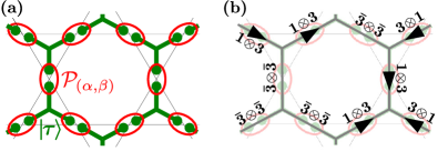
Figure 1: (a) The model is constructed from trimers $\left|\tau\right\rangle$ which are in a singlet state with representation $\mathcal{H}_{v}\equiv\bm{1}\oplus\bm{3}\oplus\bar{\bm{3}}$ at each site (green dots), to which a map $\mathcal{P}_{\bullet}$ is applied which selects the physical degrees of freedom from $\mathcal{H}_{v}\otimes\mathcal{H}_{v}$. (b) Mapping to a $\mathbb{Z}_{3}$ topological model: Each site holds a $\mathbb{Z}_{3}$ degree of freedom: one of two arrows or no arrow. The arrows are pointing towards the $\bm{3}$ representation and satisfy a Gauss law across each vertex due to the fusion rules of the $\mathrm{SU}(3)$ irreps.

We now arrange the trimers $\left|\tau\right\rangle$ as shown in Fig. 1a and apply maps $\mathcal{P}_{(\alpha,\beta)}$ to pairs of adjacent virtual sites, where the parameters $\alpha,\beta\in[0,1]$ will allow us to interpolate between the fixed point model and the $\mathrm{SU}(3)$ spin liquid. We first define the map $\mathcal{P}_{\perp}\equiv\mathcal{P}_{(1,1)}$ which projects the two adjacent sites $\mathcal{H}_{v}^{\otimes 2}=(\bm{1}\oplus\bm{3}\oplus\bar{\bm{3}})^{\otimes 2}$ onto the union of the three components $\mathcal{H}_{\omega}=\bm{1}\otimes\bm{3}$, $\mathcal{H}_{\bar{\omega}}=\bm{3}\otimes\bm{1}$, and $\mathcal{H}_{1}=\bar{\bm{3}}\otimes\bar{\bm{3}}$. We will show in a moment that the resulting wavefunction is a fixed point wavefunction with $\mathbb{Z}_{3}$ topological order.

The interpolation in $\alpha$ is now obtained by adiabatically removing the $\bar{\bm{6}}$ component in $\mathcal{H}_{1}=\bar{\bm{3}}\otimes\bar{\bm{3}}=\bm{3}\oplus\bar{\bm{6}}$, that is,

$$\mathcal{P}_{(\alpha,1)}=\Big{[}\openone_{\mathcal{H}_{\omega}}\oplus\openone_{\mathcal{H}_{\bar{\omega}}}\oplus\big{(}\alpha\openone_{\mathcal{H}_{1}}+(1-\alpha)\Pi_{\mathcal{H}_{1}^{\bm{3}}}\big{)}\Big{]}\,P_{\perp}\ ,$$ (1)

where we have decomposed $\mathcal{H}_{1}=\bm{3}\oplus\bar{\bm{6}}\equiv\mathcal{H}_{1}^{\bm{3}}\oplus\mathcal{H}_{1}^{\bar{\bm{6}}}$, and $\Pi_{\mathcal{H}}$ denotes the orthogonal projector onto $\mathcal{H}$.

At $\alpha=0$, we are left with $\mathcal{P}_{\bm{333}}=\mathcal{P}_{(0,1)}$ which maps into $\mathcal{H}_{\bm{333}}=\mathcal{H}_{\omega}\oplus\mathcal{H}_{\bar{\omega}}\oplus\mathcal{H}_{1}^{\bm{3}}\cong\bm{3}\otimes\mathbb{C}^{3}$, where the first tensor component transforms as $\bm{3}$, while the second component labels which representation we consider, and thus transforms trivially under $\mathrm{SU}(3)$. We can now remove the $\mathbb{C}^{3}$ adiabatically,

$$\mathcal{P}_{(0,\beta)}=\big{[}\openone_{\bm{3}}\otimes(\beta\,\openone_{\mathbb{C}^{3}}+(1-\beta)\left|e\right\rangle\left\langle e\right|_{\mathbb{C}^{3}})\big{]}\,\mathcal{P}_{(0,1)}\ ,$$ (2)

by projecting the label onto the equal weight superposition $\left|e\right\rangle$ of the three components (with the phases of $\mathcal{H}_{\omega}$, $\mathcal{H}_{\bar{\omega}}$ chosen opposite, leaving $\mathcal{P}_{(0,\beta)}$ antisymmetric). For $(\alpha,\beta)=(0,0)$, we can factor out the $\left|e\right\rangle$ and are thus left with an $\mathrm{SU}(3)$-invariant wavefunction (as the building blocks are $\mathrm{SU}(3)$-invariant) with the fundamental representation at each site. Clearly, the two interpolations can be combined into a two-parameter family, though in the following we will only consider the presented sequence of interpolations $(1,1)\rightarrow(0,1)\rightarrow(0,0)$.

Let us now show how to map the model with $\mathcal{P}_{(1,1)}=\mathcal{P}_{\perp}:\mathcal{H}_{v}^{\otimes 2}\rightarrow\mathcal{H}_{\omega}\oplus\mathcal{H}_{\bar{\omega}}\oplus\mathcal{H}_{1}$ to a topological $\mathbb{Z}_{3}$ fixed point model by local unitaries. To this end, let us first add an extra qutrit (“indicator”) $\{\left|-\right\rangle_{t},\left|\rightarrow\right\rangle_{t},\left|\leftarrow\right\rangle_{t}\}$ at each vertex, onto which we copy the information whether the system at that vertex is in the space $\mathcal{H}_{1}=\bar{\bm{3}}\otimes\bar{\bm{3}}$, $\mathcal{H}_{\omega}=\bm{1}\otimes\bm{3}$, or $\mathcal{H}_{\bar{\omega}}=\bm{3}\otimes\bm{1}$, as shown in Fig. 1b (the arrow always points towards the $\bm{3}$ irrep). Now consider for a moment the scenario where we project all indicator qutrits onto this basis (“classical configurations”). Given any such classical configuration, the states of the virtual system factorize into singlet states of the corresponding irreps on the individual triangles, and can thus be brought into a fiducial state by local unitaries controlled by the state of the indicator qutrits, and thus effectively removed.

This operation can be done coherently, leaving us with the indicator qutrits in a superposition of all allowed configurations. The construction of $\left|\tau\right\rangle$ ensures that around each vertex of the dual honeycomb lattice, the number of $\bm{3}$ (i.e., ingoing arrows) minus the number of $\bm{1}$ (i.e., outgoing arrows) is $0\,\mathrm{mod}\,3$. Associating the indicator qutrits with $\mathbb{Z}_{3}$ variables (with arrows pointing from the A to the B sublattice corresponding to $\omega=e^{2\pi i/3}$, the other arrows to $\bar{\omega}$, and “no arrow” to $1$), it follows that the indicator qutrits which live on the edges of the honeycomb lattice satisfy a $\mathbb{Z}_{3}$ Gauss’ law. In addition, all allowed configurations appear with equal weight. Thus, the wavefunction given by the indicator qutrits is the wavefunction of a quantum double model $D(\mathbb{Z}_{3})$, i.e., a fixed point wavefunction with $\mathbb{Z}_{3}$ topological order .

Having established that the model with $\mathcal{P}_{\perp}$ is a $\mathbb{Z}_{3}$ topological fixed point model without any long-range order in the spin degree of freedom (which we could factor out), we can now use the interpolation $\mathcal{P}_{(\alpha,\beta)}$ to study whether the topological order and the spin liquid behavior remain present all the way down to the $\mathrm{SU}(3)$ point. An important point is that along this interpolation, there exists a corresponding path of parent Hamiltonians. Continuity of the Hamiltonian, as well as the $9$-fold degenerate ground space in the finite volume (where the $9$ linearly independent ground states are obtained by placing strings of symmetry actions when closing the boundary), can be established by showing that the PEPS has a property known as $G$-injectivity Schuch et al. (2010) with $G\equiv\mathbb{Z}_{3}$, which states that (i) the tensors have a virtual $\mathbb{Z}_{3}$ symmetry – in our case, this follows directly from the fact that the number of $\bm{1}$ minus the number of $\bm{3}$ of both $\left|\tau\right\rangle$ and $\mathcal{P}_{\bullet}$ are $0\,\mathrm{mod}\,3$ – and (ii) there exists a blocking where the mapping $M$ from the virtual degrees of freedom at the boundary to the degrees of freedom in the bulk given by a patch of the PEPS is injective on the $\mathbb{Z}_{3}$-invariant subspace. We have verified that (ii) holds on a full star using full diagonalization of $M^{\dagger}M$  for all $(\alpha,\beta)$ except for $(0,0)$ . This implies the existence of a parent Hamiltonian acting on two overlapping stars, which changes continuously along the interpolation and has the correct $9$-fold degenerate ground space structure (Schuch et al., 2012, App. D). For the missing point $(\alpha,\beta)=(0,0)$, a Hamiltonian can be constructed by taking the limit of the Hamiltonians for $\alpha=0$, $\beta\rightarrow 0$, which is continuous by construction .

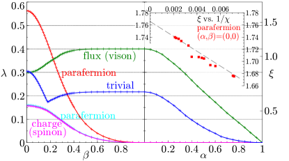
Figure 2: Anyon-anyon and trivial correlations along the interpolation $(0,0)\leftarrow(0,1)\leftarrow(1,1)$, cf. text, with $\xi$ the correlation length and $\lambda=\exp(-1/\xi)$. Data has been obtained with bond dimensions up to $\chi\sim 500$ and truncating Schmidt values down to $10^{-16}$. The data clearly shows that the $\mathrm{SU}(3)$ model is in the $D(\mathbb{Z}_{3})$ double phase. The inset shows the convergence of $\xi$ for the parafermion (red) at $(\alpha,\beta)=(0,0)$ as a function of the inverse bond dimension $1/\chi$; for large $\chi$, $\xi$ exhibits the linear scaling commonly found for PEPS in this extrapolation, yielding an approximate value of $\xi\approx 1.77$.

III Numerical study

Let us now study the behavior along the interpolation. To this end, we use infinite MPS (iMPS) with tunable bond dimension $\chi$ to approximate the fixed point of the PEPS transfer operator Haegeman and Verstraete (2017). From the iMPS, we can obtain correlation lengths $\xi_{g,\eta}$ for general anyon-anyon correlations through the subleading eigenvalues $\lambda_{g,\eta}=\exp[-1/\xi_{g,\eta}]$ of the (dressed) iMPS transfer operator Iqbal et al. (2018). Here, group elements $g$ label anyon fluxes, and irreps $\eta$ label anyon charges. These describe different types of excitations: Fluxes or visons correspond to an incorrect relative weight of different singlet configurations, and charges or spinons to a spinful excitation (i.e., a breaking of singlets); they are modeled by strings of symmetry actions and irrep actions on the virtual level, respectively. Composite particles of visons and spinons possess a parafermionic $e^{\pm 2\pi i/3}$ statistics. The numerical results for these quantities along the interpolation are shown in Fig. 2. We find that for the first part of the interpolation, $(1,1)\to(0,1)$, only vison excitations acquire a finite correlation length. This can be understood from the fact that projecting out the $\bar{\bm{6}}$ component in $\bar{\bm{3}}\otimes\bar{\bm{3}}=\bm{3}\oplus\bar{\bm{6}}$ decreases the effective amplitude of singlets with $\bar{\bm{3}}$ representations. In fact, these correlations can be mostly supressed by considering a modified model where $\mathcal{P}_{(\alpha,1)}$, Eq. (1), carries an additional factor in front of the $(1-\alpha)$ term to keep the total weight of the $\bar{\bm{3}}\otimes\bar{\bm{3}}$ subspace fixed; we term this the $\bar{\bm{3}}$-enhanced model and discuss it in more detail in the Appendix. Along the second interpolation $(0,1)\to(0,0)$, we observe that the vison length does no longer grow (and ultimately even decreases), while the length scale towards the $\mathrm{SU}(3)$ point is dominated by one of the parafermions. At the $\mathrm{SU}(3)$ point, we find $\xi\approx 1.77$ by extrapolating in $1/\chi$ . Most importantly, the extrapolation clearly shows that the correlation length for $\chi\to\infty$ is finite, even if one might prefer to take the precise extrapolated value with a bit of care. The fact that there is no divergence in any correlation thus proves that the system is gapped, and in the same phase as the $\mathbb{Z}_{3}$ quantum double model, with no anyons condensed Duivenvoorden et al. (2017); Iqbal et al. (2018). This is confirmed by the convergence analysis shown in the inset, and is consistent with a number of other checks . For the $\bar{\bm{3}}$-enhanced model (Fig. 4a), we find a strongly decreased correlation length along the $\alpha$-interpolation, as expected. Surprisingly, this effect is reversed along the $\beta$-interpolation, and at the $\mathrm{SU}(3)$ point, $\xi\approx 2.64$. Nevertheless, the results conclusively show that this model is in the $D(\mathbb{Z}_{3})$ phase as well.

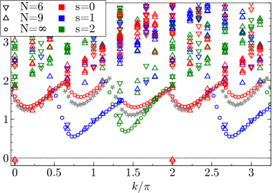
Figure 3: Entanglement spectrum of the $\mathrm{SU}(3)$ model, computed from the iMPS fixed point exactly for $N=6,9$ and using an iMPS excitation ansatz for $N=\infty$, labelled by $\mathbb{Z}_{3}$ symmetry sectors $s=0,1,2$. Finite $N$ spectra are trace-normalized per sector, and shifted by the leading eigenvalue in the thermodynamic limit. The gray stars indicate the lower edge of the two-particle continuum computed from the $s=1$ and $s=2$ one-particle branches for $N=\infty$. The interactions between the particles determine the finite-size energies of these two-particle states; the fact that for $N=6,9$ we only see the continuum around momentum zero indicates that the interactions are attractive only in that region. The fact that the $N=\infty$ quasiparticle-ansatz in that region yields results close to the two-particle edge (as compared to the other two edges) confirms this picture.

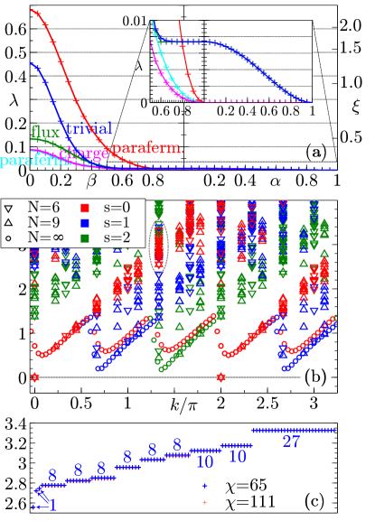
Figure 4: The $\bar{\bm{3}}$-enhanced model. (a) Correlation functions (cf. Fig. 2). (b) Entanglement spectrum (cf. Fig. 3). Here, the finite $N$ data in the trivial sector is scaled to leading eigenvalue $0$, and the relative normalization of the other sectors is shifted by a factor $1.5$ such as to match the $N=\infty$ data. Just as in Fig. 3, we can see that the finite-size data only contains the momentum zero two-particle edge. This, together with the counting, suggests that the states on this edge will evolve towards an elementary chiral mode when the state approaches the critical point. (c) The multiplet of lowest eigenvalues in the ES at $k=4\times(2\pi/N)$, $N=6$ (ellipse in (b)), computed using two iMPS approximations with $\chi=65,111$. We perfectly recover the $\mathrm{SU}(3)_{1}$ counting Di Francesco et al. (1997) without having imposed any symmetries. We also observe that the ES only depends very weakly on the iMPS bond dimension $\chi$.

The fact that our wavefunction transforms chirally under the lattice symmetry raises the question whether it might display a chiral ES (i.e., an ES described by a chiral CFT). We have studied the ES of the model at the $\mathrm{SU}(3)$ point using an iMPS fixed point of the transfer operator with $\chi=59$, using (i) exact diagonalization on cylinders up to circumference $N=9$ (which reveals a $3$-periodicity), and (ii) an iMPS excitation ansatz in the thermodynamic limit ($N=\infty)$ Haegeman et al. (2015); Haegeman and Verstraete (2017). The results for $N=6,9,\infty$ are shown in Fig. 3, labeled by their $\mathbb{Z}_{3}$ sector. On the one hand, one can clearly see that the ES breaks time-reversal and exhibits clear right-moving modes for all three branches. On the other hand, it also becomes clear from the $N=9$ and $N=\infty$ data that the ES is gapped, with a much steeper left-moving mode. (This is confirmed by computing the momentum polarization Tu et al. (2013) from the iMPS Poilblanc et al. (2016).) These features become more pronounced when considering the ES for the $\bar{\bm{3}}$-enhanced model (Fig. 4b). In that case, the lowest branches become clearly separated from the rest of the spectrum, allowing to perform a counting of the spin multiplets. The results in the trivial sector are in full agreement with the counting and spin multiplet structure for a chiral $\mathrm{SU}(3)_{1}$ CFT for at least the first $5$ levels (Fig. 4c). Nevertheless, inclusion of the $N=9$ and $N=\infty$ data strongly indicates that the ES is still gapped.

IV Conclusions

In conclusion, we have presented a PEPS model which realizes a $\mathrm{SU}(3)$ TSL with $\mathbb{Z}_{3}$ topological order, and comprehensively characterized its topological and entanglement properties. A number of questions remain: First, it would be interesting to see whether twisted versions of the model can be built without breaking lattice symmetries; this seems plausible given the unbiased nature of the mapping to the topological $\mathbb{Z}_{3}$ model. Second, the model transforms chirally under reflection, which seems unavoidable since different singlets in $\left|\tau\right\rangle$ transform differently under reflection (and removing either kind results in a critical or trivial model); it would thus be interesting to clarify whether there are fundamental obstacles for constructing a trivially transforming $\mathrm{SU}(3)$ spin liquid. Third, the connection to realistic systems is up for further study. In the case of $\mathrm{SU}(2)$, the motivation for considering RVBs originates in the search for spin liquids in (frustrated) Heisenberg models, and the question arises how our PEPS construction can serve a similar purpose for $\mathrm{SU}(N)$. Although the simplest $\mathrm{SU}(N)$ Heisenberg models seem to form symmetry broken simplex solids Corboz et al. (2012), one can look for additional spin interactions that stabilize spin liquids of the form that we presented , or try to invoke the connection between PEPS and two-body Hamiltonians through perturbative constructions Brell et al. (2011). An alternative route towards experimental implementations could be to devise schemes for the controlled dynamical preparation of such wavefunctions in e.g. optical lattices, using for instance the connection between PEPS and perturbative constructions. Finally, a natural follow-up question is to investigate whether the model can be further deformed to acquire a chiral $\mathrm{SU}(3)_{1}$ ES, e.g. by further increasing the weight of the $\bar{\bm{3}}$, and whether this happens at the transition into the trivial phase, as well as to to better understand its relation to other chiral models with $\mathrm{SU}(3)_{1}$ ES Wu and Tu (2016); Nataf et al. (2016).

Acknowledgements

We acknowledge helpful discussions with I. Cirac, A. Hackenbroich, D. Poilblanc, A. Sterdyniak, and H.-H. Tu. This work has been supported by the EU through the ERC Starting Grant WASCOSYS (No. 636201), and by the Flemish Research Foundation.

Appendix: The $\bar{\bm{3}}$-enhanced model

In this Appendix, we describe the construction of the $\bar{\bm{3}}$-enhanced model and provide numerical results on its correlation functions, entanglement spectrum, and CFT counting of the ES.

The model is constructed in complete analogy to the original model introduced in the main text, with the difference that the interpolation $\mathcal{P}_{(\alpha,1)}$ is constructed such as to keep the total weight of the $\bar{\bm{3}}\otimes\bar{\bm{3}}$ subspace constant along the interpolation (in which we continuously remove the $\bm{\bar{6}}$ component in $\bar{\bm{3}}\otimes\bar{\bm{3}}=3\oplus\bm{\bar{6}}$). Specifically, this amounts to replacing Eq. (1) by

$$\mathcal{P}^{\prime}_{(\alpha,1)}=\Big{[}\openone_{\mathcal{H}_{\omega}}\oplus\openone_{\mathcal{H}_{\bar{\omega}}}\oplus\big{(}\alpha\openone_{\mathcal{H}_{1}}+(\sqrt{3-2\alpha^{2}}-\alpha)\Pi_{\mathcal{H}_{1}^{\bm{3}}}\big{)}\Big{]}\,P_{\perp}\ . \ref{eq:first-P-interpolation}^{\prime}$$ ()

Correspondingly, $\mathcal{P}_{(0,\beta)}$, Eq. (2), needs to be modified by replacing $\mathcal{P}_{(0,1)}$ on the r.h.s. by

$$\mathcal{P}^{\prime}_{(0,1)}=\Big{[}\openone_{\mathcal{H}_{\omega}}\oplus\openone_{\mathcal{H}_{\bar{\omega}}}\oplus\sqrt{3}\,\Pi_{\mathcal{H}_{1}^{\bm{3}}}\Big{]}\,P_{\perp}\ .$$

The analysis of the correlations, shown in Fig. 4a, reveals that the modification indeed succeeds in decreasing the correlation length significantly during the $\alpha$-interpolation. On the other hand, we find that as we approach the $\mathrm{SU}(3)$ invariant point along the $\beta$-interpolation, the effect is reversed, and the final correlation length at the $\mathrm{SU}(3)$ invariant point $\beta=0$ is in fact larger than for the original model, $\xi\approx 2.64$. This can be understood from the fact that the deformation increases the weight of the $\bar{\bm{3}}\otimes\bar{\bm{3}}\otimes\bar{\bm{3}}$ configuration in $\tau$, which will ultimately drive the system through a transition into a trivial phase.

The entanglement spectrum of the $\bar{\bm{3}}$-enhanced model, shown in Fig. 4b, exhibits a much more pronounced difference between the left- and right-propagating modes, suggesting that the model might eventually become chiral when further increasing the weight of the $\bar{\bm{3}}$ configurations, possibly at the phase transition. The clearly separated right-moving branches allows for the identification and counting of the spin multiplets for a given momentum $k=2\pi n/N$, which we find to perfectly match the counting of the $\mathrm{SU}(3)_{1}$ CFT. For illustration, the $n=4$ multiplet is shown in Fig. 4c.

References

- Anderson (1987) P. W. Anderson, Science 235, 1196 (1987).
- Moessner and Sondhi (2001) R. Moessner and S. L. Sondhi, Phys. Rev. Lett. 86, 1881 (2001), cond-mat/0007378 .
- Misguich et al. (2002) G. Misguich, D. Serban, and V. Pasquier, Phys. Rev. Lett. 89, 137202 (2002), cond-mat/0204428 .
- Verstraete and Cirac (2004) F. Verstraete and J. I. Cirac, Phys. Rev. A 70, 060302 (2004), quant-ph/0311130 .
- Schuch et al. (2012) N. Schuch, D. Poilblanc, J. I. Cirac, and D. Pérez-García, Phys. Rev. B 86, 115108 (2012), arXiv:1203.4816 .
- Hackenbroich et al. (2018) A. Hackenbroich, A. Sterdyniak, and N. Schuch, (2018), arXiv:1805.04531 .
- Schuch et al. (2010) N. Schuch, I. Cirac, and D. Pérez-García, Ann. Phys. 325, 2153 (2010), arXiv:1001.3807 .
- Iqbal et al. (2014) M. Iqbal, D. Poilblanc, and N. Schuch, Phys. Rev. B 90, 115129 (2014), 1407.7773 .
- Qi et al. (2015) Y. Qi, Z.-C. Gu, and H. Yao, Phys. Rev. B 92, 155105 (2015), arXiv:1406.6364 .
- Buerschaper et al. (2014) O. Buerschaper, S. C. Morampudi, and F. Pollmann, Phys. Rev. B 90, 195148 (2014), arXiv:1407.8521 .
- Zaletel and Vishwanath (2015) M. P. Zaletel and A. Vishwanath, Phys. Rev. Lett. 114, 077201 (2015), arXiv:1410.2894 .
- Gorshkov et al. (2010) A. V. Gorshkov, M. Hermele, V. Gurarie, C. Xu, P. S. Julienne, J. Ye, P. Zoller, E. Demler, M. D. Lukin, and A. M. Rey, Nature Phys. 6, 289 (2010), arXiv:0905.2610 .
- Scazza et al. (2014) F. Scazza, C. Hofrichter, M. Höfer, P. C. D. Groot, I. Bloch, and S. Fölling, Nature Phys. 10, 779 (2014), arXiv:1403.4761 .
- Zhang et al. (2014) X. Zhang, M. Bishof, S. L. Bromley, C. V. Kraus, M. S. Safronova, P. Zoller, A. M. Rey, and J. Ye, Science 345, 1467 (2014), arXiv:1403.2964 .
- Hermele and Gurarie (2011) M. Hermele and V. Gurarie, Phys. Rev. B 84, 174441 (2011), arXiv:1108.3862 .
- Nataf et al. (2016) P. Nataf, M. Lajko, A. Wietek, K. Penc, F. Mila, and A. M. Laeuchli, Phys. Rev. Lett. 117, 167202 (2016), arXiv:1601.00958 .
- Note (1) Observe that our model is not a “resonating trimer state” as e.g. in Ref. Lee et al. (2017), since projecting creates large entangled clusters (e.g. for the vaccuum of the model). Placing the model of Ref. Lee et al. (2017) on the kagome lattice in fact yields a variant of our model with a modified which we found to be in a trivial phase.
- Note (2) Using conservation and rewriting as a product of matrices each depending on the virtual ket+bra indices on one tip of the star; note that it is sufficient to check this for , since for , can be mapped to by acting on the physical system.
- Note (3) The latter point might still be -injective, but this would require checking larger patches which seems numerically prohibitive.
- Note (4) The existence of the limit is guaranteed by the fact that the parent Hamiltonian is constructed as the projector onto the orthocomplement of the image of the PEPS on two overlapping stars, which is a polynomial (and thus analytic) map in , together with the fact that eigenspace projectors of analytic hermitian matrices are analytic themselves ((Kato, 1966, Thm. 6.1)).
- Haegeman and Verstraete (2017) J. Haegeman and F. Verstraete, Annual Review of Condensed Matter Physics 8, 355 (2017), arXiv:1611.08519 .
- Iqbal et al. (2018) M. Iqbal, K. Duivenvoorden, and N. Schuch, Phys. Rev. B 97, 195124 (2018), arXiv:1712.04021 .
- Note (5) The longest-ranging two-point correlations (corresponding to the trivial sector) with are obtained for spin-spin correlations.
- Duivenvoorden et al. (2017) K. Duivenvoorden, M. Iqbal, J. Haegeman, F. Verstraete, and N. Schuch, Phys. Rev. B 95, 235119 (2017), arXiv:1702.08469 .
- Note (6) Exact diagonalization of the transfer operator on small cylinders, the convergence of the iMPS method, and the smooth change of the leading eigenvalue and eigenvector of the transfer operator along the interpolation.
- Haegeman et al. (2015) J. Haegeman, V. Zauner, N. Schuch, and F. Verstraete, Nature Comm. 6, 8284 (2015), arXiv:1410.5443 .
- Tu et al. (2013) H.-H. Tu, Y. Zhang, and X.-L. Qi, Phys. Rev. B 88, 195412 (2013), arXiv:1212.6951 .
- Poilblanc et al. (2016) D. Poilblanc, N. Schuch, and I. Affleck, Phys. Rev. B 93, 174414 (2016), arXiv:1602.05969 .
- Corboz et al. (2012) P. Corboz, K. Penc, F. Mila, and A. M. Laeuchli, Phys. Rev. B 86, 041106 (2012), arXiv:1204.6682 .
- Note (7) Note that similarly, also AKLT-type constructions for higher exhibit symmetry breaking Arovas (2008), so that it is an interesting question whether our construction for higher (at least is straightforward) will eventually cease to give a spin liquid.
- Brell et al. (2011) C. G. Brell, S. T. Flammia, S. D. Bartlett, and A. C. Doherty, New J. Phys. 13, 053039 (2011), arXiv:1011.1942 .
- Wu and Tu (2016) Y.-H. Wu and H.-H. Tu, Phys. Rev. B 94, 201113 (2016), arXiv:1601.02594 .
- Lee et al. (2017) H. Lee, Y. Oh, J. H. Han, and H. Katsura, Phys. Rev. B 95, 060413 (2017), arXiv:1612.06899 .
- Kato (1966) T. Kato, Perturbation theory for linear operators (Springer Berlin Heidelberg, 1966).
- Arovas (2008) D. P. Arovas, Phys. Rev. B 77, 104404 (2008), arXiv:0711.3921 .
- Di Francesco et al. (1997) P. Di Francesco, P. Mathieu, and D. Sénéchal, Conformal Field Theory, Graduate Texts in Contemporary Physics (Springer, 1997).