On gradient regularizers for MMD GANs
Abstract
We propose a principled method for gradient-based regularization of the critic of GAN-like models trained by adversarially optimizing the kernel of a Maximum Mean Discrepancy (MMD). We show that controlling the gradient of the critic is vital to having a sensible loss function, and devise a method to enforce exact, analytical gradient constraints at no additional cost compared to existing approximate techniques based on additive regularizers. The new loss function is provably continuous, and experiments show that it stabilizes and accelerates training, giving image generation models that outperform state-of-the art methods on CelebA and unconditional ImageNet.
1 Introduction
There has been an explosion of interest in implicit generative models (IGMs) over the last few years, especially after the introduction of generative adversarial networks (GANs) [16]. These models allow approximate samples from a complex high-dimensional target distribution , using a model distribution , where estimation of likelihoods, exact inference, and so on are not tractable. GAN-type IGMs have yielded very impressive empirical results, particularly for image generation, far beyond the quality of samples seen from most earlier generative models [[, e.g.]]progressive-growing,dcgan,wgan-gp,munit,anime-gans.
These excellent results, however, have depended on adding a variety of methods of regularization and other tricks to stabilize the notoriously difficult optimization problem of GANs [42, 38]. Some of this difficulty is perhaps because when a GAN is viewed as minimizing a discrepancy , its gradient does not provide useful signal to the generator if the target and model distributions are not absolutely continuous, as is nearly always the case [2].
An alternative set of losses are the integral probability metrics (IPMs) [36], which can give credit to models “near” to the target distribution \parenciteswganBottou:2017[Section 4 of][]GneRaf07. IPMs are defined in terms of a critic function: a “well behaved” function with large amplitude where and differ most. The IPM is the difference in the expected critic under and , and is zero when the distributions agree. The Wasserstein IPMs, whose critics are made smooth via a Lipschitz constraint, have been particularly successful in IGMs [3, 18, 14]. But the Lipschitz constraint must hold uniformly, which can be hard to enforce. A popular approximation has been to apply a gradient constraint only in expectation [18]: the critic’s gradient norm is constrained to be small on points chosen uniformly between and .
Another class of IPMs used as IGM losses are the Maximum Mean Discrepancies (MMDs) [17], as in [28, 13]. Here the critic function is a member of a reproducing kernel Hilbert space (except in [50], who learn a deep approximation to an RKHS critic). Better performance can be obtained, however, when the MMD kernel is not based directly on image pixels, but on learned features of images. Wasserstein-inspired gradient regularization approaches can be used on the MMD critic when learning these features: [27] uses weight clipping [3], and [7, 5] use a gradient penalty [18].
The recent Sobolev GAN [33] uses a similar constraint on the expected gradient norm, but phrases it as estimating a Sobolev IPM rather than loosely approximating Wasserstein. This expectation can be taken over the same distribution as [18], but other measures are also proposed, such as . A second recent approach, the spectrally normalized GAN [32], controls the Lipschitz constant of the critic by enforcing the spectral norms of the weight matrices to be 1. Gradient penalties also benefit GANs based on -divergences [37]: for instance, the spectral normalization technique of [32] can be applied to the critic network of an -GAN. Alternatively, a gradient penalty can be defined to approximate the effect of blurring and with noise [40], which addresses the problem of non-overlapping support [2]. This approach has recently been shown to yield locally convergent optimization in some cases with non-continuous distributions, where the original GAN does not [30].
In this paper, we introduce a novel regularization for the MMD GAN critic of [5, 27, 7], which directly targets generator performance, rather than adopting regularization methods intended to approximate Wasserstein distances [3, 18]. The new MMD regularizer derives from an approach widely used in semi-supervised learning [[]Section 2]Bousquet:2004, where the aim is to define a classification function which is positive on (the positive class) and negative on (negative class), in the absence of labels on many of the samples. The decision boundary between the classes is assumed to be in a region of low density for both and : should therefore be flat where and have support (areas with constant label), and have a larger slope in regions of low density. [10] propose as their regularizer on a sum of the variance and a density-weighted gradient norm.
We adopt a related penalty on the MMD critic, with the difference that we only apply the penalty on : thus, the critic is flatter where has high mass, but does not vanish on the generator samples from (which we optimize). In excluding from the critic function constraint, we also avoid the concern raised by [32] that a critic depending on will change with the current minibatch – potentially leading to less stable learning. The resulting discrepancy is no longer an integral probability metric: it is asymmetric, and the critic function class depends on the target being approximated.
2 Learning implicit generative models with MMD-based losses
An IGM is a model which aims to approximate a target distribution over a space . We will define by a generator function , implemented as a deep network with parameters , where is a space of latent codes, say . We assume a fixed distribution on , say , and call the distribution of . We will consider learning by minimizing a discrepancy between distributions, with and , which we call our loss. We aim to minimize with stochastic gradient descent on an estimator of .
In the present work, we will build losses based on the Maximum Mean Discrepancy,
| (1) |
an integral probability metric where the critic class is the unit ball within , the reproducing kernel Hilbert space with a kernel . The optimization in (1) admits a simple closed-form optimal critic, . There is also an unbiased, closed-form estimator of with appealing statistical properties [17] – in particular, its sample complexity is independent of the dimension of , compared to the exponential dependence [52] of the Wasserstein distance
| (2) |
The MMD is continuous in the weak topology for any bounded kernel with Lipschitz embeddings [46, Theorem 3.2(b)], meaning that if converges in distribution to , , then . ( is continuous in the slightly stronger Wasserstein topology [51, Definition 6.9]; implies , and the two notions coincide if is bounded.) Continuity means the loss can provide better signal to the generator as approaches , as opposed to e.g. Jensen-Shannon where the loss could be constant until suddenly jumping to 0 [[, e.g.]Example 1]wgan. The MMD is also strict, meaning it is zero iff , for characteristic kernels [45]. The Gaussian kernel yields an MMD both continuous in the weak topology and strict. Thus in principle, one need not conduct any alternating optimization in an IGM at all, but merely choose generator parameters to minimize .
Despite these appealing properties, using simple pixel-level kernels leads to poor generator samples [13, 28, 48, 8]. More recent MMD GANs [27, 5, 7] achieve better results by using a parameterized family of kernels, , in the Optimized MMD loss previously studied by [44, 46]:
| (3) |
We primarily consider kernels defined by some fixed kernel on top of a learned low-dimensional representation , i.e. , denoted . In practice, is a simple characteristic kernel, e.g. Gaussian, and is usually a deep network with output dimension say [7] or even (in our experiments). If is powerful enough, this choice is sufficient; we need not try to ensure each is characteristic, as did [27].
Proposition 1.
Suppose , with characteristic and rich enough that for any , there is a for which .111 denotes the pushforward of a distribution: if , then . Then if , .
Proof.
Let be such that . Then, since is characteristic,
To estimate , one can conduct alternating optimization to estimate a and then update the generator according to , similar to the scheme used in GANs and WGANs. (This form of estimator is justified by an envelope theorem [31], although it is invariably biased [7].) Unlike or , fixing a and optimizing the generator still yields a sensible distance .
Early attempts at minimizing in an IGM, though, were unsuccessful [48, footnote 7]. This could be because for some kernel classes, is stronger than Wasserstein or MMD.
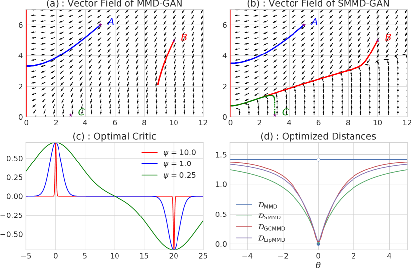
Example 1 (DiracGAN [30]).
We wish to model a point mass at the origin of , , with any possible point mass, for . We use a Gaussian kernel of any bandwidth, which can be written as with for and . Then
Considering , even though , shows that the Optimized MMD distance is not continuous in the weak or Wasserstein topologies.
This also causes optimization issues. Figure 1 (a) shows gradient vector fields in parameter space, . Some sequences following (e.g. A) converge to an optimal solution , but some (B) move in the wrong direction, and others (C) are stuck because there is essentially no gradient. Figure 1 (c, red) shows that the optimal critic is very sharp near and ; this is less true for cases where the algorithm converged.
We can avoid these issues if we ensure a bounded Lipschitz critic:222[27, Theorem 4] makes a similar claim to 2, but its proof was incorrect: it tries to uniformly bound , but the bound used is for a Wasserstein in terms of .
Proposition 2.
Assume the critics are uniformly bounded and have a common Lipschitz constant: and . In particular, this holds when and
Then is continuous in the weak topology: if , then .
Proof.
The main result is [12, Corollary 11.3.4]. To show the claim for , note that , which since is
Indeed, if we put a box constraint on [27] or regularize the gradient of the critic function [7], the resulting MMD GAN generally matches or outperforms WGAN-based models. Unfortunately, though, an additive gradient penalty doesn’t substantially change the vector field of Figure 1 (a), as shown in Figure 5 (Appendix B). We will propose distances with much better convergence behavior.
3 New discrepancies for learning implicit generative models
Our aim here is to introduce a discrepancy that can provide useful gradient information when used as an IGM loss. Proofs of results in this section are deferred to Appendix A.
3.1 Lipschitz Maximum Mean Discrepancy
2 shows that an MMD-like discrepancy can be continuous under the weak topology even when optimizing over kernels, if we directly restrict the critic functions to be Lipschitz. We can easily define such a distance, which we call the Lipschitz MMD: for some ,
| (4) |
For a universal kernel , we conjecture that . But for any and , is upper-bounded by , as (4) optimizes over a smaller set of functions than (2). Thus is also upper-bounded by , and hence is continuous in the Wasserstein topology. It also shows excellent empirical behavior on Example 1 (Figure 1 (d), and Figure 5 in Appendix B). But estimating , let alone , is in general extremely difficult (Appendix D), as finding requires optimization in the input space. Constraining the mean gradient rather than the maximum, as we will do next, is far more tractable.
3.2 Gradient-Constrained Maximum Mean Discrepancy
We define the Gradient-Constrained MMD for and using some measure as
| (5) | ||||
| (6) |
denotes the squared norm. Rather than directly constraining the Lipschitz constant, the second term encourages the function to be flat where has mass. In experiments we use , flattening the critic near the target sample. We add the first term following [10]: in one dimension and with uniform, is then an RKHS norm with the kernel , which is also a Sobolev space. The correspondence to a Sobolev norm is lost in higher dimensions [[]Ch. 10]Wendland05, but we also found the first term to be beneficial in practice.
We can exploit some properties of to compute (5) analytically. Call the difference in kernel mean embeddings ; recall .
Proposition 3.
Let . Define with th entry , and with th entry333We use to denote ; thus stacks , …, into one vector. . Then under Assumptions (A), (B), (C) and (D) in Section A.1,
where is the kernel matrix , is the matrix of left derivatives 444We use to denote the partial derivative with respect to , and that for . , and that of derivatives of both arguments .
As long as and have integrable first moments, and has second moments, Assumptions (A), (B), (C) and (D) are satisfied e.g. by a Gaussian or linear kernel on top of a differentiable . We can thus estimate the GCMMD based on samples from , , and by using the empirical mean for .
This discrepancy indeed works well in practice: Section F.2 shows that optimizing our estimate of yields a good generative model on MNIST. But the linear system of size is impractical: even on images and using a low-rank approximation, the model took days to converge. We therefore design a less expensive discrepancy in the next section.
The GCMMD is related to some discrepancies previously used in IGM training. The Fisher GAN [34] uses only the variance constraint . The Sobolev GAN [33] constrains , along with a vanishing boundary condition on to ensure a well-defined solution (although this was not used in the implementation, and can cause very unintuitive critic behavior; see Appendix C). The authors considered several choices of , including the WGAN-GP measure [18] and mixtures . Rather than enforcing the constraints in closed form as we do, though, these models used additive regularization. We will compare to the Sobolev GAN in experiments.
3.3 Scaled Maximum Mean Discrepancy
We will now derive a lower bound on the Gradient-Constrained MMD which retains many of its attractive qualities but can be estimated in time linear in the dimension .
Proposition 4.
Make Assumptions (A), (B), (C) and (D). For any , , where
We then define the Scaled Maximum Mean Discrepancy based on this bound of 4:
| (7) |
Because the constraint in the optimization of (7) is more restrictive than in that of (5), we have that . The Sobolev norm , and a fortiori the gradient norm under , is thus also controlled for the SMMD critic. We also show in Section F.1 that behaves similarly to on Gaussians.
If and , then . Or if is linear, , then . Estimating these terms based on samples from is straightforward, giving a natural estimator for the SMMD.
Of course, if and are fixed, the SMMD is simply a constant times the MMD, and so behaves in essentially the same way as the MMD. But optimizing the SMMD over a kernel family , , gives a distance very different from (3).
Figure 1 (b) shows the vector field for the Optimized SMMD loss in Example 1, using the WGAN-GP measure . The optimization surface is far more amenable: in particular the location , which formerly had an extremely small gradient that made learning effectively impossible, now converges very quickly by first reducing the critic gradient until some signal is available. Figure 1 (d) demonstrates that , like and but in sharp contrast to , is continuous with respect to the location and provides a strong gradient towards 0.
We can establish that is continuous in the Wasserstein topology under some conditions:
Theorem 1.
Let , with a fully-connected -layer network with Leaky-ReLUα activations whose layers do not increase in width, and satisfying mild smoothness conditions (Assumptions (II), (III), (IV) and (V) in Section A.2). Let be the set of parameters where each layer’s weight matrices have condition number . If has a density (Assumption (I)), then
Thus if , then , even if is chosen to depend on and .
Uniform bounds vs bounds in expectation
Controlling does not necessarily imply a bound on , and so does not in general give continuity via 2. Theorem 1 implies that when the network’s weights are well-conditioned, it is sufficient to only control , which is far easier in practice than controlling .
If we instead tried to directly controlled with e.g. spectral normalization (SN) [32], we could significantly reduce the expressiveness of the parametric family. In Example 1, constraining limits us to only . Thus is simply the with an RBF kernel of bandwidth 1, which has poor gradients when is far from (Figure 1 (c), blue). The Cauchy-Schwartz bound of 4 allows jointly adjusting the smoothness of and the critic , while SN must control the two independently. Relatedly, limiting by limiting the Lipschitz norm of each layer could substantially reduce capacity, while need not be decomposed by layer. Another advantage is that provides a data-dependent measure of complexity as in [10]: we do not needlessly prevent ourselves from using critics that behave poorly only far from the data.
Spectral parametrization
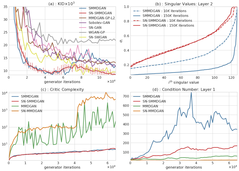
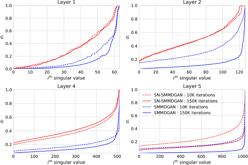
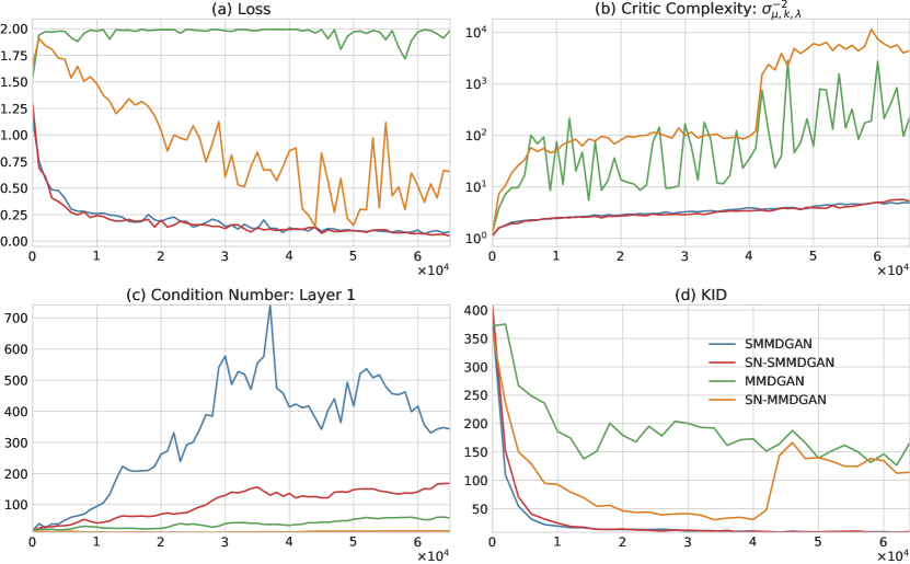
When the generator is near a local optimum, the critic might identify only one direction on which and differ. If the generator parameterization is such that there is no local way for the generator to correct it, the critic may begin to single-mindedly focus on this difference, choosing redundant convolutional filters and causing the condition number of the weights to diverge. If this occurs, the generator will be motivated to fix this single direction while ignoring all other aspects of the distributions, after which it may become stuck. We can help avoid this collapse by using a critic parameterization that encourages diverse filters with higher-rank weight matrices. [32] propose to parameterize the weight matrices as , where is the spectral norm of . This parametrization works particularly well with ; Figure 2 (b) shows the singular values of the second layer of a critic’s network (and Figure 9, in Section F.3, shows more layers), while Figure 2 (d) shows the evolution of the condition number during training. The conditioning of the weight matrix remains stable throughout training with spectral parametrization, while it worsens through training in the default case.
4 Experiments
We evaluated unsupervised image generation on three datasets: CIFAR-10 [26] ( images, ), CelebA [29] ( face images, resized and cropped to as in [7]), and the more challenging ILSVRC2012 (ImageNet) dataset [41] ( images, resized to ). Code for all of these experiments is available at github.com/MichaelArbel/Scaled-MMD-GAN.
Losses All models are based on a scalar-output critic network , except MMDGAN-GP where as in [7]. The WGAN and Sobolev GAN use a critic , while the GAN uses a discriminator . The MMD-based methods use a kernel , except for MMDGAN-GP which uses a mixture of RQ kernels as in [7]. Increasing the output dimension of the critic or using a different kernel didn’t substantially change the performance of our proposed method. We also consider SMMD with a linear top-level kernel, ; because this becomes essentially identical to a WGAN (Appendix E), we refer to this method as SWGAN. SMMD and SWGAN use ; Sobolev GAN uses as in [33]. We choose and an overall scaling to obtain the losses:
Architecture For CIFAR-10, we used the CNN architecture proposed by [32] with a 7-layer critic and a 4-layer generator. For CelebA, we used a 5-layer DCGAN discriminator and a 10-layer ResNet generator as in [7]. For ImageNet, we used a 10-layer ResNet for both the generator and discriminator. In all experiments we used filters for the smallest convolutional layer, and double it at each layer (CelebA/ImageNet) or every other layer (CIFAR-10). The input codes for the generator are drawn from . We consider two parameterizations for each critic: a standard one where the parameters can take any real value, and a spectral parametrization (denoted SN-) as above [32]. Models without explicit gradient control (SN-GAN, SN-MMDGAN, SN-MMGAN-L2, SN-WGAN) fix , for spectral normalization; others learn , using a spectral parameterization.
Training All models were trained for generator updates on a single GPU, except for ImageNet where the model was trained on 3 GPUs simultaneously. To limit communication overhead we averaged the MMD estimate on each GPU, giving the block MMD estimator [54]. We always used samples per GPU from each of and , and critic updates per generator step. We used initial learning rates of for CIFAR-10 and CelebA, for ImageNet, and decayed these rates using the KID adaptive scheme of [7]: every steps, generator samples are compared to those from steps ago, and if the relative KID test [9] fails to show an improvement three consecutive times, the learning rate is decayed by . We used the Adam optimizer [25] with , .
Evaluation To compare the sample quality of different models, we considered three different scores based on the Inception network [49] trained for ImageNet classification, all using default parameters in the implementation of [7]. The Inception Score (IS) [42] is based on the entropy of predicted labels; higher values are better. Though standard, this metric has many issues, particularly on datasets other than ImageNet [4, 20, 7]. The FID [20] instead measures the similarity of samples from the generator and the target as the Wasserstein-2 distance between Gaussians fit to their intermediate representations. It is more sensible than the IS and becoming standard, but its estimator is strongly biased [7]. The KID [7] is similar to FID, but by using a polynomial-kernel MMD its estimates enjoy better statistical properties and are easier to compare. (A similar score was recommended by [21].)
| CIFAR-10 | CelebA | |||||
|---|---|---|---|---|---|---|
| Method | IS | FID | KID | IS | FID | KID |
| WGAN-GP | 6.90.2 | 31.10.2 | 22.21.1 | 2.70.0 | 29.20.2 | 22.01.0 |
| MMDGAN-GP-L2 | 6.90.1 | 31.40.3 | 23.31.1 | 2.60.0 | 20.50.2 | 13.01.0 |
| Sobolev-GAN | 7.00.1 | 30.30.3 | 22.31.2 | 2.90.0 | 16.40.1 | 10.60.5 |
| SMMDGAN | 7.00.1 | 31.50.4 | 22.21.1 | 2.70.0 | 18.40.2 | 11.50.8 |
| SN-GAN | 7.20.1 | 26.70.2 | 16.10.9 | 2.70.0 | 22.60.1 | 14.61.1 |
| SN-SWGAN | 7.20.1 | 28.50.2 | 17.61.1 | 2.80.0 | 14.10.2 | 7.70.5 |
| SN-SMMDGAN | 7.30.1 | 25.00.3 | 16.62.0 | 2.80.0 | 12.40.2 | 6.10.4 |
| Method | IS | FID | KID |
|---|---|---|---|
| BGAN | 10.70.4 | 43.90.3 | 47.01.1 |
| SN-GAN | 11.20.1 | 47.50.1 | 44.42.2 |
| SMMDGAN | 10.70.2 | 38.40.3 | 39.32.5 |
| SN-SMMDGAN | 10.90.1 | 36.60.2 | 34.61.6 |
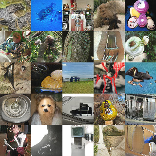


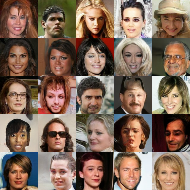
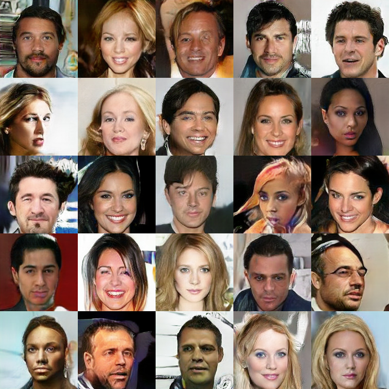

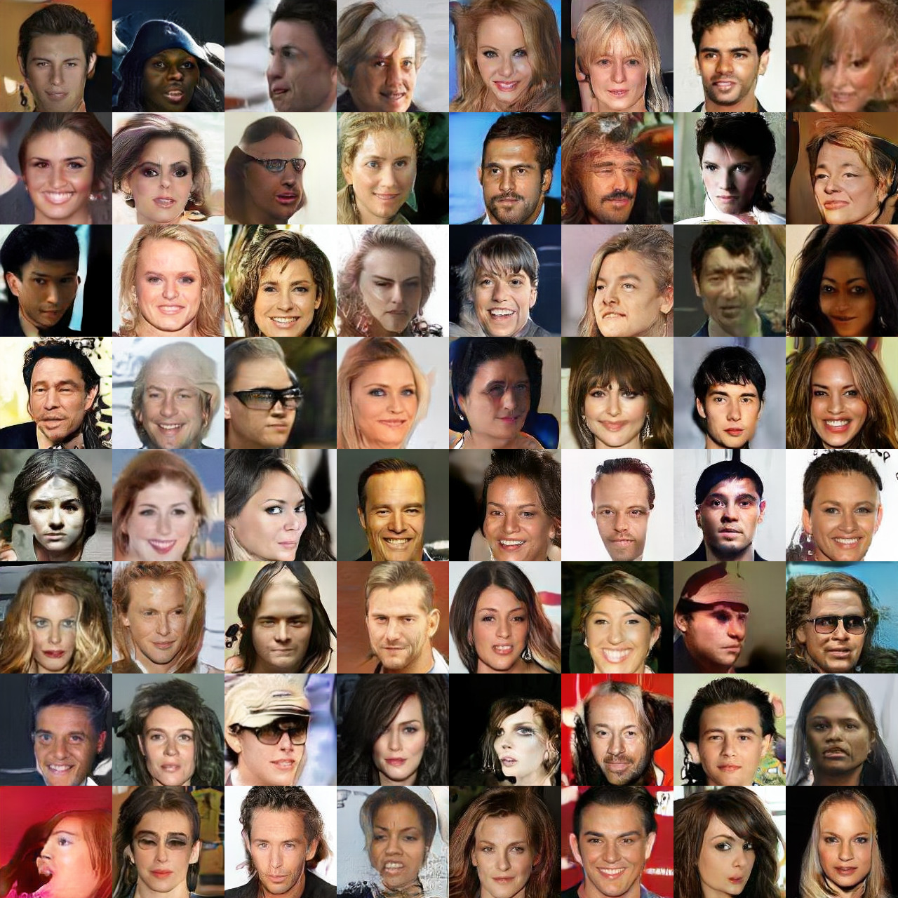
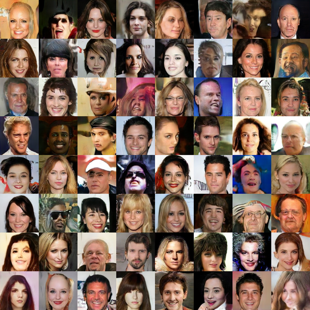
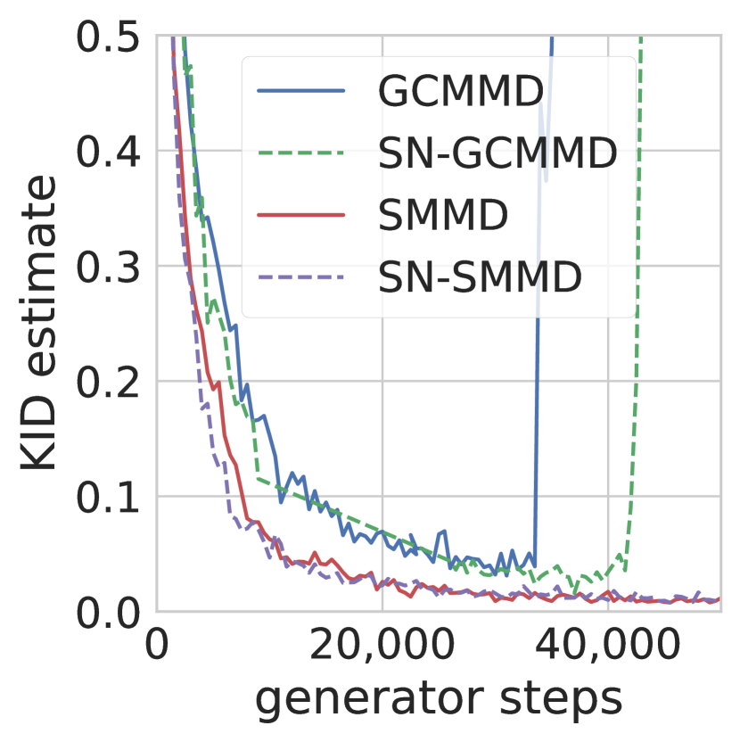
Results Table 1(a) presents the scores for models trained on both CIFAR-10 and CelebA datasets. On CIFAR-10, SN-SWGAN and SN-SMMDGAN performed comparably to SN-GAN. But on CelebA, SN-SWGAN and SN-SMMDGAN dramatically outperformed the other methods with the same architecture in all three metrics. It also trained faster, and consistently outperformed other methods over multiple initializations (Figure 2 (a)). It is worth noting that SN-SWGAN far outperformed WGAN-GP on both datasets. Table 1(b) presents the scores for SMMDGAN and SN-SMMDGAN trained on ImageNet, and the scores of pre-trained models using BGAN [6] and SN-GAN [32].555These models are courtesy of the respective authors and also trained at resolution. SN-GAN used the same architecture as our model, but trained for generator iterations; BS-GAN used a similar 5-layer ResNet architecture and trained for 74 epochs, comparable to SN-GAN. The proposed methods substantially outperformed both methods in FID and KID scores. Figure 3 shows samples on ImageNet and CelebA; Section F.4 has more.
Spectrally normalized WGANs / MMDGANs To control for the contribution of the spectral parametrization to the performance, we evaluated variants of MMDGANs, WGANs and Sobolev-GAN using spectral normalization (in Table 2, Section F.3). WGAN and Sobolev-GAN led to unstable training and didn’t converge at all (Figure 11) despite many attempts. MMDGAN converged on CIFAR-10 (Figure 11) but was unstable on CelebA (Figure 10). The gradient control due to SN is thus probably too loose for these methods. This is reinforced by Figure 2 (c), which shows that the expected gradient of the critic network is much better-controlled by SMMD, even when SN is used. We also considered variants of these models with a learned while also adding a gradient penalty and an penalty on critic activations [7, footnote 19]. These generally behaved similarly to MMDGAN, and didn’t lead to substantial improvements. We ran the same experiments on CelebA, but aborted the runs early when it became clear that training was not successful.
Rank collapse We occasionally observed the failure mode for SMMD where the critic becomes low-rank, discussed in Section 3.3, especially on CelebA; this failure was obvious even in the training objective. Figure 2 (b) is one of these examples. Spectral parametrization seemed to prevent this behavior. We also found one could avoid collapse by reverting to an earlier checkpoint and increasing the RKHS regularization parameter , but did not do this for any of the experiments here.
5 Conclusion
We studied gradient regularization for MMD-based critics in implicit generative models, clarifying how previous techniques relate to the loss. Based on these insights, we proposed the Gradient-Constrained MMD and its approximation the Scaled MMD, a new loss function for IGMs that controls gradient behavior in a principled way and obtains excellent performance in practice.
One interesting area of future study for these distances is their behavior when used to diffuse particles distributed as towards particles distributed as . [33, Appendix A.1] began such a study for the Sobolev GAN loss; [35] proved convergence and studied discrete-time approximations.
Another area to explore is the geometry of these losses, as studied by [8], who showed potential advantages of the Wasserstein geometry over the MMD. Their results, though, do not address any distances based on optimized kernels; the new distances introduced here might have interesting geometry of their own.
pages40 rangepages20 rangepages19 rangepages15 rangepages5 rangepages22 rangepages55
References
- [1] Brandon Amos and J. Kolter “OptNet: Differentiable Optimization as a Layer in Neural Networks” In ICML, 2017 arXiv:1703.00443
- [2] M. Arjovsky and L. Bottou “Towards Principled Methods for Training Generative Adversarial Networks” In ICLR, 2017 arXiv:1701.04862
- [3] M. Arjovsky, S. Chintala and L. Bottou “Wasserstein Generative Adversarial Networks” In ICML, 2017 arXiv:1701.07875
- [4] Shane Barratt and Rishi Sharma “A Note on the Inception Score”, 2018 arXiv:1801.01973
- [5] M.. Bellemare, I. Danihelka, W. Dabney, S. Mohamed, B. Lakshminarayanan, S. Hoyer and R. Munos “The Cramer Distance as a Solution to Biased Wasserstein Gradients”, 2017 arXiv:1705.10743
- [6] D. Berthelot, T. Schumm and L. Metz “BEGAN: Boundary Equilibrium Generative Adversarial Networks”, 2017 arXiv:1703.10717
- [7] Mikołaj Bińkowski, Dougal J. Sutherland, Michael Arbel and Arthur Gretton “Demystifying MMD GANs” In ICLR, 2018 arXiv:1801.01401
- [8] Léon Bottou, Martin Arjovsky, David Lopez-Paz and Maxime Oquab “Geometrical Insights for Implicit Generative Modeling” In Braverman Readings in Machine Learning: Key Iedas from Inception to Current State, LNAI Vol. 11100 Springer, 2018, pp. 229–268 arXiv:1712.07822
- [9] W. Bounliphone, E. Belilovsky, M.. Blaschko, I. Antonoglou and A. Gretton “A Test of Relative Similarity For Model Selection in Generative Models” In ICLR, 2016 arXiv:1511.04581
- [10] Olivier Bousquet, Olivier Chapelle and Matthias Hein “Measure Based Regularization” In NIPS, 2004
- [11] Andrew Brock, Theodore Lim, J.. Ritchie and Nick Weston “Neural Photo Editing with Introspective Adversarial Networks” In ICLR, 2017 arXiv:1609.07093
- [12] Richard M. Dudley “Real Analysis and Probability” Cambridge University Press, 2002
- [13] G.. Dziugaite, D.. Roy and Z. Ghahramani “Training generative neural networks via Maximum Mean Discrepancy optimization” In UAI, 2015 arXiv:1505.03906
- [14] Aude Genevay, Gabriel Peyré and Marco Cuturi “Learning Generative Models with Sinkhorn Divergences” In AISTATS, 2018 arXiv:1706.00292
- [15] T. Gneiting and A.. Raftery “Strictly proper scoring rules, prediction, and estimation” In JASA 102.477, 2007, pp. 359–378
- [16] I. Goodfellow, J. Pouget-Abadie, M. Mirza, B. Xu, D. Warde-Farley, S. Ozair, A. Courville and Y. Bengio “Generative Adversarial Nets” In NIPS, 2014 arXiv:1406.2661
- [17] A. Gretton, K.. Borgwardt, M.. Rasch, B. Schölkopf and A.. Smola “A Kernel Two-Sample Test” In JMLR 13, 2012
- [18] I. Gulrajani, F. Ahmed, M. Arjovsky, V. Dumoulin and A. Courville “Improved Training of Wasserstein GANs” In NIPS, 2017 arXiv:1704.00028
- [19] A.Dilek Güngör “Some bounds for the product of singular values” In International Journal of Contemporary Mathematical Sciences, 2007
- [20] M. Heusel, H. Ramsauer, T. Unterthiner, B. Nessler, G. Klambauer and S. Hochreiter “GANs Trained by a Two Time-Scale Update Rule Converge to a Nash Equilibrium” In NIPS, 2017 arXiv:1706.08500
- [21] Gao Huang, Yang Yuan, Qiantong Xu, Chuan Guo, Yu Sun, Felix Wu and Kilian Weinberger “An empirical study on evaluation metrics of generative adversarial networks”, 2018 arXiv:1806.07755
- [22] Xun Huang, Ming-Yu Liu, Serge Belongie and Jan Kautz “Multimodal Unsupervised Image-to-Image Translation” In ECCV, 2018 arXiv:1804.04732
- [23] Y. Jin, K. Zhang, M. Li, Y. Tian, H. Zhu and Z. Fang “Towards the Automatic Anime Characters Creation with Generative Adversarial Networks”, 2017 arXiv:1708.05509
- [24] Tero Karras, Timo Aila, Samuli Laine and Jaakko Lehtinen “Progressive Growing of GANs for Improved Quality, Stability, and Variation” In ICLR, 2018 arXiv:1710.10196
- [25] D. Kingma and J. Ba “Adam: A Method for Stochastic Optimization” In ICLR, 2015 arXiv:1412.6980
- [26] A. Krizhevsky “Learning Multiple Layers of Features from Tiny Images”, 2009
- [27] C.-L. Li, W.-C. Chang, Y. Cheng, Y. Yang and B. Póczos “MMD GAN: Towards Deeper Understanding of Moment Matching Network” In NIPS, 2017 arXiv:1705.08584
- [28] Y. Li, K. Swersky and R. Zemel “Generative Moment Matching Networks” In ICML, 2015 arXiv:1502.02761
- [29] Z. Liu, P. Luo, X. Wang and X. Tang “Deep learning face attributes in the wild” In ICCV, 2015 arXiv:1411.7766
- [30] Lars Mescheder, Andreas Geiger and Sebastian Nowozin “Which Training Methods for GANs do actually Converge?” In ICML, 2018 arXiv:1801.04406
- [31] P. Milgrom and I. Segal “Envelope theorems for arbitrary choice sets” In Econometrica 70.2, 2002, pp. 583–601
- [32] Takeru Miyato, Toshiki Kataoka, Masanori Koyama and Yuichi Yoshida “Spectral Normalization for Generative Adversarial Networks” In ICLR, 2018 arXiv:1802.05927
- [33] Youssef Mroueh, Chung-Liang Li, Tom Sercu, Anant Raj and Yu Cheng “Sobolev GAN” In ICLR, 2018 arXiv:1711.04894
- [34] Youssef Mroueh and Tom Sercu “Fisher GAN” In NIPS, 2017 arXiv:1705.09675
- [35] Youssef Mroueh, Tom Sercu and Anant Raj “Regularized Kernel and Neural Sobolev Descent: Dynamic MMD Transport”, 2018 arXiv:1805.12062
- [36] A. Müller “Integral Probability Metrics and their Generating Classes of Functions” In Advances in Applied Probability 29.2, 1997, pp. 429–443
- [37] S. Nowozin, B. Cseke and R. Tomioka “f-GAN: Training Generative Neural Samplers using Variational Divergence Minimization” In NIPS, 2016 arXiv:1606.00709
- [38] A. Radford, L. Metz and S. Chintala “Unsupervised Representation Learning with Deep Convolutional Generative Adversarial Networks” In ICLR, 2016 arXiv:1511.06434
- [39] J.. Retherford “Review: J. Diestel and J. J. Uhl, Jr., Vector measures” In Bull. Amer. Math. Soc. 84.4 American Mathematical Society, 1978, pp. 681–685
- [40] Kevin Roth, Aurelien Lucchi, Sebastian Nowozin and Thomas Hofmann “Stabilizing Training of Generative Adversarial Networks through Regularization” In NIPS, 2017 arXiv:1705.09367
- [41] Olga Russakovsky et al. “ImageNet Large Scale Visual Recognition Challenge”, 2014 arXiv:1409.0575
- [42] T. Salimans, I. Goodfellow, W. Zaremba, V. Cheung, A. Radford and X. Chen “Improved Techniques for Training GANs” In NIPS, 2016 arXiv:1606.03498
- [43] John Shawe-Taylor and Nello Cristianini “Kernel Methods for Pattern Analysis” Cambridge University Press, 2004
- [44] B.. Sriperumbudur, K. Fukumizu, A. Gretton, G… Lanckriet and B. Schölkopf “Kernel choice and classifiability for RKHS embeddings of probability distributions” In NIPS, 2009
- [45] B.. Sriperumbudur, K. Fukumizu and G… Lanckriet “Universality, Characteristic Kernels and RKHS Embedding of Measures” In JMLR 12, 2011, pp. 2389–2410 arXiv:1003.0887
- [46] Bharath Sriperumbudur “On the optimal estimation of probability mesaures in weak and strong topologies” In Bernoulli 22.3, 2016, pp. 1839–1893 arXiv:1310.8240
- [47] I. Steinwart and A. Christmann “Support Vector Machines” Springer, 2008
- [48] D.. Sutherland, H.-Y. Tung, H. Strathmann, S. De, A. Ramdas, A. Smola and A. Gretton “Generative Models and Model Criticism via Optimized Maximum Mean Discrepancy” In ICLR, 2017 arXiv:1611.04488
- [49] C. Szegedy, V. Vanhoucke, S. Ioffe, J. Shlens and Z. Wojna “Rethinking the Inception Architecture for Computer Vision” In CVPR, 2016 arXiv:1512.00567
- [50] Thomas Unterthiner, Bernhard Nessler, Calvin Seward, Günter Klambauer, Martin Heusel, Hubert Ramsauer and Sepp Hochreiter “Coulomb GANs: Provably Optimal Nash Equilibria via Potential Fields” In ICLR, 2018 arXiv:1708.08819
- [51] Cedric Villani “Optimal Transport: Old and New” Springer, 2009
- [52] Jonathan Weed and Francis Bach “Sharp asymptotic and finite-sample rates of convergence of empirical measures in Wasserstein distance” In Bernoulli, forthcoming arXiv:1707.00087
- [53] H. Wendland “Scattered Data Approximation” Cambridge University Press, 2005
- [54] W. Zaremba, A. Gretton and M.. Blaschko “B-tests: Low Variance Kernel Two-Sample Tests” In NIPS, 2013 arXiv:1307.1954
Appendix A Proofs
We first review some basic properties of Reproducing Kernel Hilbert Spaces. We consider here a separable RKHS with basis , where is either finite if is finite-dimensional, or otherwise. We also assume that the reproducing kernel is continuously twice differentiable.
We use a slightly nonstandard notation for derivatives: denotes the th partial derivative of evaluated at , and denotes .
Then the following reproducing properties hold for any given function in [47, Lemma 4.34]:
| (8) | ||||
| (9) |
We say that an operator is Hilbert-Schmidt if is finite. is called the Hilbert-Schmidt norm of . The space of Hilbert-Schmidt operators itself a Hilbert space with the inner product . Moreover, we say that an operator is trace-class if its trace norm is finite, i.e. . The outer product for gives an operator such that for all in .
Given two vectors and in and a Hilbert-Schmidt operator we have the following properties:
-
(i)
The outer product is a Hilbert-Schmidt operator with Hilbert-Schmidt norm given by: .
-
(ii)
The inner product between two rank-one operators and is .
-
(iii)
The following identity holds: .
A.1 Definitions and estimators of the new distances
We will need the following assumptions about the distributions and , the measure , and the kernel :
-
(A)
and have integrable first moments.
-
(B)
grows at most linearly in : for all in , for some constant .
-
(C)
The kernel is twice continuously differentiable.
-
(D)
The functions and for are -integrable.
When , Assumption (B) is automatically satisfied by a such as the Gaussian; when is linear, it is true for a quite general class of networks [7, Lemma 1].
Proposition 5.
Under Assumptions (A), (B), (C) and (D), the Gradient-Constrained MMD is given by
| (11) |
Proof of 5.
Let be a function in . We will first express the squared -regularized Sobolev norm of (6) as a quadratic form in . Recalling the reproducing properties of (8) and (9), we have:
Using Property (ii) and the operator (10), one further gets
Under Assumption (D), and using 6, one can take the integral inside the inner product, which leads to . Finally, using Property (iii) it follows that
Under Assumptions (A) and (B), 6 applies, and it follows that is also Bochner integrable under and . Thus
where is defined as this difference in mean embeddings.
Since is symmetric positive definite, its square-root is well-defined and is also invertible. For any , let , so that . Note that for any , there is a corresponding . Thus we can re-express the maximization problem in (5) in terms of :
5, though, involves inverting the infinite-dimensional operator and thus doesn’t directly give us a computable estimator. 3 solves this problem in the case where is a discrete measure:
Proposition 3.
Let be an empirical measure of points. Let have th entry , and have th entry666We use to denote ; thus stacks , …, into one vector. . Then under Assumptions (A), (B), (C) and (D), the Gradient-Constrained MMD is
where is the kernel matrix , is the matrix of left derivatives , and that of derivatives of both arguments .
Before proving 3, we note the following interesting alternate form. Let be the th standard basis vector for , and define as the linear operator
Then , and . Thus we can write
Proof of 3.
Let be the solution to the regression problem :
| (12) |
Taking the inner product of both sides of (12) with for each yields the following equations:
| (13) |
Doing the same with gives equations:
| (14) |
From (12), it is clear that is a linear combination of the form:
where the coefficients and satisfy the system of equations (13) and (14). We can rewrite this system as
where , are the identity matrices of dimension , . Since and must be positive semidefinite, an inverse exists. We conclude by noticing that
The following result was key to our definition of the SMMD in Section 3.3.
Proposition 4.
Proof of 4.
The key idea here is to use the Cauchy-Schwarz inequality for the Hilbert-Schmidt inner product. Letting , is
follows from the reproducing properties (8) and (9) and Property (ii). is obtained using Property (iii), while follows from the Cauchy-Schwarz inequality and Property (i). ∎
Lemma 6.
Under Assumption (D), is Bochner integrable and its integral is a trace-class symmetric positive semi-definite operator with invertible for any positive . Moreover, for any Hilbert-Schmidt operator we have: .
Under Assumptions (A) and (B), is Bochner integrable with respect to any probability distribution with finite first moment and the following relation holds: for all in .
Proof.
The operator is positive self-adjoint. It is also trace-class, as by the triangle inequality
By Assumption (D), we have that which implies that is -integrable in the Bochner sense [39, Definition 1 and Theorem 2]. Its integral is trace-class and satisfies . This allows to have for all Hilbert-Schmidt operators . Moreover, the integral preserves the symmetry and positivity. It follows that is invertible.
The Bochner integrability of under a distribution with finite moment follows directly from Assumptions (A) and (B), since . This allows us to write . ∎
A.2 Continuity of the Optimized Scaled MMD in the Wasserstein topology
To prove Theorem 1, we we will first need some new notation.
We assume the kernel is , i.e. , where the representation function is a network consisting of fully-connected layers:
| (15) | ||||
The intermediate representations are of dimension , the weights are matrices in , and biases are vectors in . The elementwise activation function is given by , and for the activation is a leaky ReLU with leak coefficient :
| (16) |
The parameter is the concatenation of all the layer parameters:
We denote by the set of all such possible parameters, i.e. . Define the following restrictions of :
| (17) | ||||
| (18) |
is the set of those parameters such that have a small condition number, . is the set of per-layer normalized parameters with a condition number bounded by .
Recall the definition of Scaled MMD, Equation 7, where and is a probability measure:
The Optimized SMMD over the restricted set is given by:
The constraint to is critical to the proof. In practice, using a spectral parametrization helps enforce this assumption, as shown in Figures 2 and 9. Other regularization methods, like orthogonal normalization [11], are also possible.
We will use the following assumptions:
-
(I)
is a probability distribution absolutely continuous with respect to the Lebesgue measure.
-
(II)
The dimensions of the weights are decreasing per layer: for all .
-
(III)
The non-linearity used is Leaky-ReLU, (16), with leak coefficient .
-
(IV)
The top-level kernel is globally Lipschitz in the RKHS norm: there exists a positive constant such that for all and in .
-
(V)
There is some for which satisfies
(19)
Assumption (I) ensures that the points where is not differentiable are reached with probability under . This assumption can be easily satisfied e.g. if we define by adding Gaussian noise to .
Assumption (II) helps ensure that the span of is never contained in the null space of . Using Leaky-ReLU as a non-linearity, Assumption (III), further ensures that the network is locally full-rank almost everywhere; this might not be true with ReLU activations, where it could be always . Assumptions (II) and (III) can be easily satisfied by design of the network.
Assumptions (IV) and (V) only depend on the top-level kernel and are easy to satisfy in practice. In particular, they always hold for a smooth translation-invariant kernel, such as the Gaussian, as well as the linear kernel.
We are now ready to prove Theorem 1.
Theorem 1.
Proof.
Define the pseudo-distance corresponding to the kernel
Denote by the optimal transport metric between and using the cost , given by
where is the set of couplings with marginals and . By 7,
Recall that is Lipschitz, , so along with Assumption (IV) we have that
Thus
where is the standard Wasserstein distance (2), and so
We have that where the middle term is a matrix and the outer terms are vectors of length . Thus Assumption (V) implies that , and hence
so that
Using 8, we can write with . Then we have
where we used . But by 9, for Lebesgue-almost all , . Using Assumption (I), this implies that
Thus for any ,
The desired bound on follows immediately. ∎
Lemma 7.
Let be the continuous kernel of an RKHS defined on a Polish space , and define the corresponding pseudo-distance . Then the following inequality holds for any distributions and on , including when the quantities are infinite:
Proof.
Let and be two probability distributions, and let be the set of couplings between them. Let be an optimal coupling, which is guaranteed to exist [51, Theorem 4.1]; by definition . When the inequality trivially holds, so assume that .
Take a sample and a function with . By the Cauchy-Schwarz inequality,
Taking the expectation with respect to , we obtain
The right-hand side is just the definition of . By Jensen’s inequality, the left-hand side is lower-bounded by
since has marginals and . We have shown so far that for any with ,
the result follows by taking the supremum over . ∎
Lemma 8.
Let . There exists a corresponding scalar and , defined by (18), such that for all ,
Proof.
Set , , and . Note that the condition number is unchanged, , and , so . It is also easy to see from (16) that
so that
Lemma 9.
Make Assumptions (II) and (III), and let . Then the set of inputs for which any intermediate activation is exactly zero,
has zero Lebesgue measure. Moreover, for any , exists and
Proof.
First, note that the network representation at layer is piecewise affine. Specifically, define by, using Assumption (III),
it is undefined when any , i.e. when . Let . Then
and thus
| (20) |
where , , and , so long as .
Because , we have and ; also, , . Thus , and using Assumption (II) with 10 gives . In particular, each is full-rank.
Next, note that and each only depend on through the activation patterns . Letting denote the full activation patterns up to level , we can thus write
There are only finitely many possible values for ; we denote the set of such values as . Then we have that
Because each is of rank , each set in the union is either empty or an affine subspace of dimension . As each , each set in the finite union has zero Lebesgue measure, and also has zero Lebesgue measure.
We will now show that the activation patterns are piecewise constant, so that for all . Because , we have , and in particular
Thus, take some , and find the smallest absolute value of its activations, ; clearly . For any with , we know that for all and ,
implying that as well as . Thus for any point , . Finally, we obtain
Lemma 10.
Let , , with . Then .
Proof.
A more general version of this result can be found in [19, Theorem 2]; we provide a proof here for completeness.
If has a nontrivial null space, and the inequality holds. Otherwise, let denote . Recall that for with ,
Thus, as for ,
A.2.1 When some of the assumptions don’t hold
Here we analyze through simple examples what happens when the condition number can be unbounded, and when Assumption (II), about decreasing widths of the network, is violated.
Condition Number:
We start by a first example where the condition number can be arbitrarily high. We consider a two-layer network on , defined by
| (21) |
where . As approaches the matrix becomes singular which means that its condition number blows up. We are interested in analyzing the behavior of the Lipschitz constant of and the expected squared norm of its gradient under as approaches .
One can easily compute the squared norm of the gradient of which is given by
| (22) |
Here , , and are defined by Equation 23 and are represented in Figure 4:
| (23) | ||||
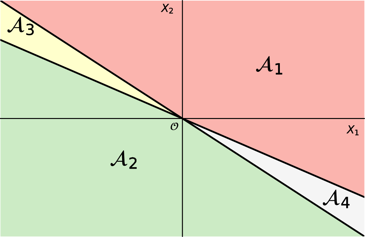
It is easy to see that whenever has a density, the probability of the sets and goes to are . Hence one can deduce that when . On the other hand, the squared Lipschitz constant of is given by which converges to . This shows that controlling the expectation of the gradient doesn’t allow to effectively control the Lipschitz constant of .
Monotonicity of the dimensions:
We would like to consider a second example where Assumption (II) doesn’t hold. Consider the following two layer network defined by:
| (24) |
for . Note that is a full rank matrix, but Assumption (II) doesn’t hold. Depending on the sign of the components of one has the following expression for :
| (25) |
where are defined by Equation 26
| (26) | ||||
The squared Lipschitz constant is given by while the expected squared norm of the gradient of is given by:
| (27) |
Again the set becomes negligible as approaches which implies that . On the other hand converges to . Note that unlike in the first example in Equation 21, the matrix has a bounded condition number. In this example, the columns of are all in the null space of , which implies for all , even though all matrices have full rank.
Appendix B DiracGAN vector fields for more losses
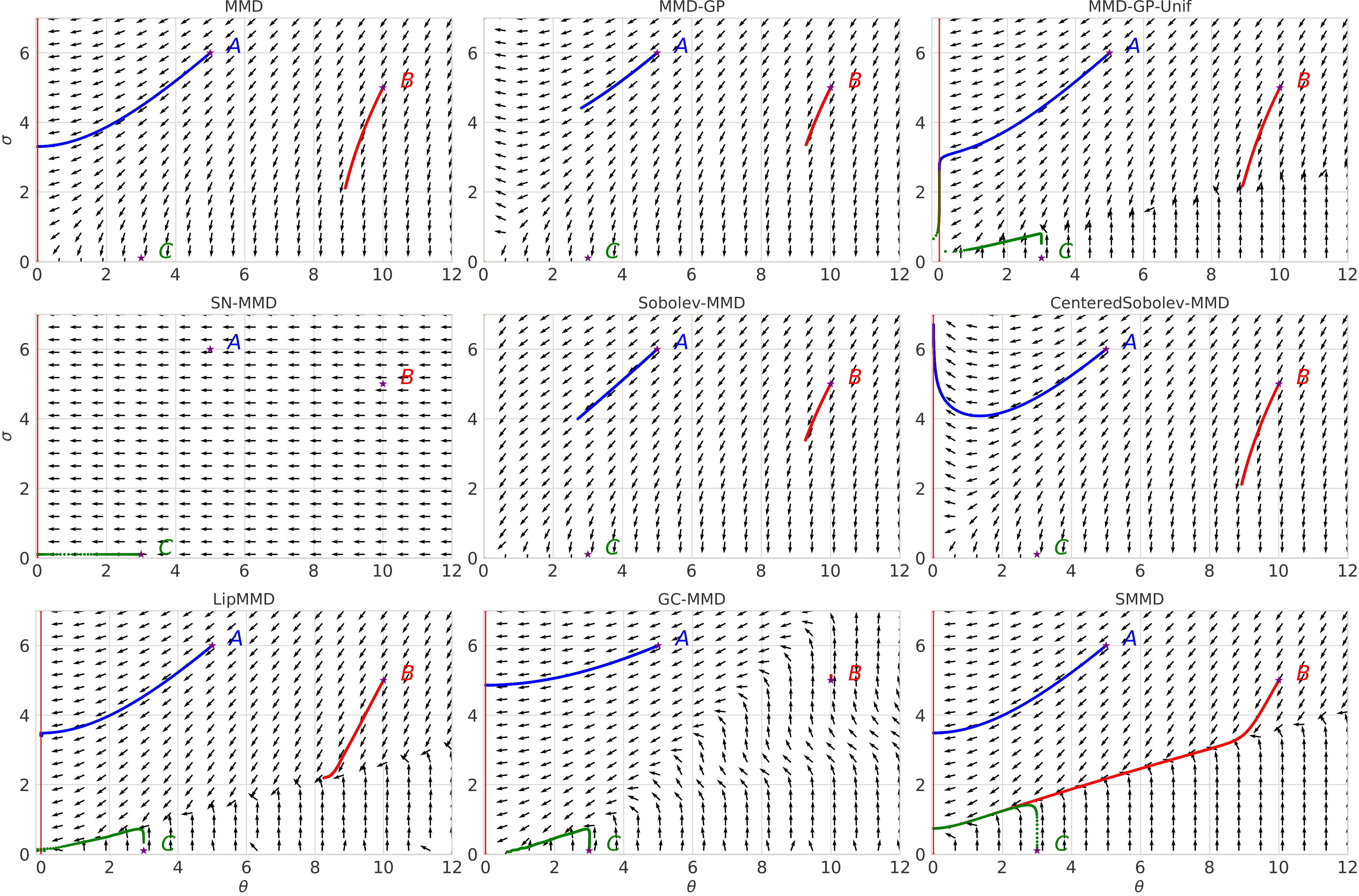
Figure 5 shows parameter vector fields, like those in Figure 6, for Example 1 for a variety of different losses:
| (28) | ||||
The squared MMD between and under a Gaussian kernel of bandwidth and is given by . MMD-GP-unif uses a gradient penalty as in [7] where each samples from is obtained by first sampling and from and and then sampling uniformly between and . MMD-GP uses the same gradient penalty, but the expectation is taken under rather than . SN-MMD refers to MMD with spectral normalization; here this means that . Sobolev-MMD refers to the loss used in [33] with the quadratic penalty only. is defined by Equation 5, with .
Appendix C Vector fields of Gradient-Constrained MMD and Sobolev GAN critics
[33] argue that the gradient of the critic (…) defines a transportation plan for moving the distribution mass (from generated to reference distribution) and present the solution of Sobolev PDE for 2-dimensional Gaussians. We observed that in this simple example the gradient of the Sobolev critic can be very high outside of the areas of high density, which is not the case with the Gradient-Constrained MMD. Figure 6 presents critic gradients in both cases, using for both.
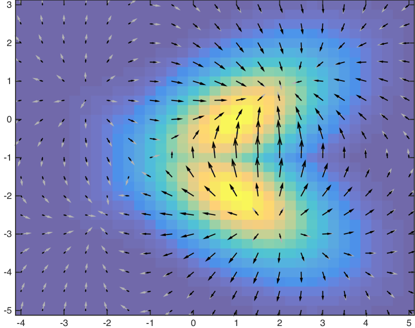
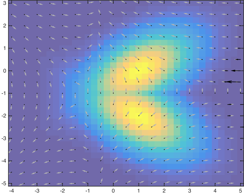
This unintuitive behavior is most likely related to the vanishing boundary condition, assummed by Sobolev GAN. Solving the actual Sobolev PDE, we found that the Sobolev critic has very high gradients close to the boundary in order to match the condition; moreover, these gradients point in opposite directions to the target distribution.
Appendix D An estimator for Lipschitz MMD
We now describe briefly how to estimate the Lipschitz MMD in low dimensions. Recall that
For , it is the case that
Thus we can approximate the constraint by enforcing the constraint on a set of points reasonably densely covering the region around the supports of and , rather than enforcing it at every point in . An estimator of the Lipschitz MMD based on and is
| (29) |
By the generalized representer theorem, the optimal for (29) will be of the form
Writing , the objective function is linear in ,
The constraints are quadratic, built from the following matrices, where the and samples are concatenated together, as are the derivatives with each dimension of the samples:
Given these matrices, and letting where is the th standard basis vector in , we have that
Thus the optimization problem (29) is a linear problem with convex quadratic constraints, which can be solved by standard convex optimization software. The approximation is reasonable only if we can effectively cover the region of interest with densely spaced ; it requires a nontrivial amount of computation even for the very simple 1-dimensional toy problem of Example 1.
One advantage of this estimator, though, is that finding its derivative with respect to the input points or the kernel parameterization is almost free once we have computed the estimate, as long as our solver has computed the dual variables corresponding to the constraints in (29). We just need to exploit the envelope theorem and then differentiate the KKT conditions, as done for instance in [1]. The differential of (29) ends up being, assuming the optimum of (29) is at and ,
Appendix E Near-equivalence of WGAN and linear-kernel MMD GANs
For an MMD GAN-GP with kernel , we have that
and the corresponding critic function is
Thus if we assume , as that is the goal of our critic training, we see that the MMD becomes identical to the WGAN loss, and the gradient penalty is applied to the same function.
(MMD GANs, however, would typically train on the unbiased estimator of , giving a very slightly different loss function. [7] also applied the gradient penalty to rather than the true critic .)
The SMMD with a linear kernel is thus analogous to applying the scaling operator to a WGAN; hence the name SWGAN.
Appendix F Additional experiments
F.1 Comparison of Gradient-Constrained MMD to Scaled MMD
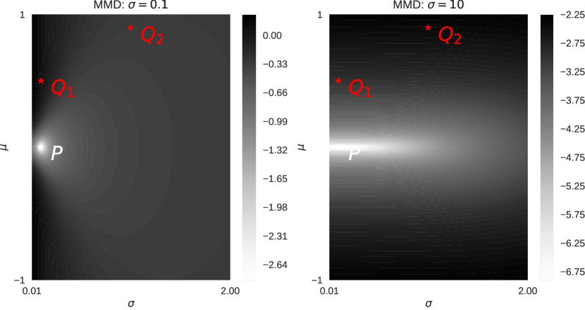
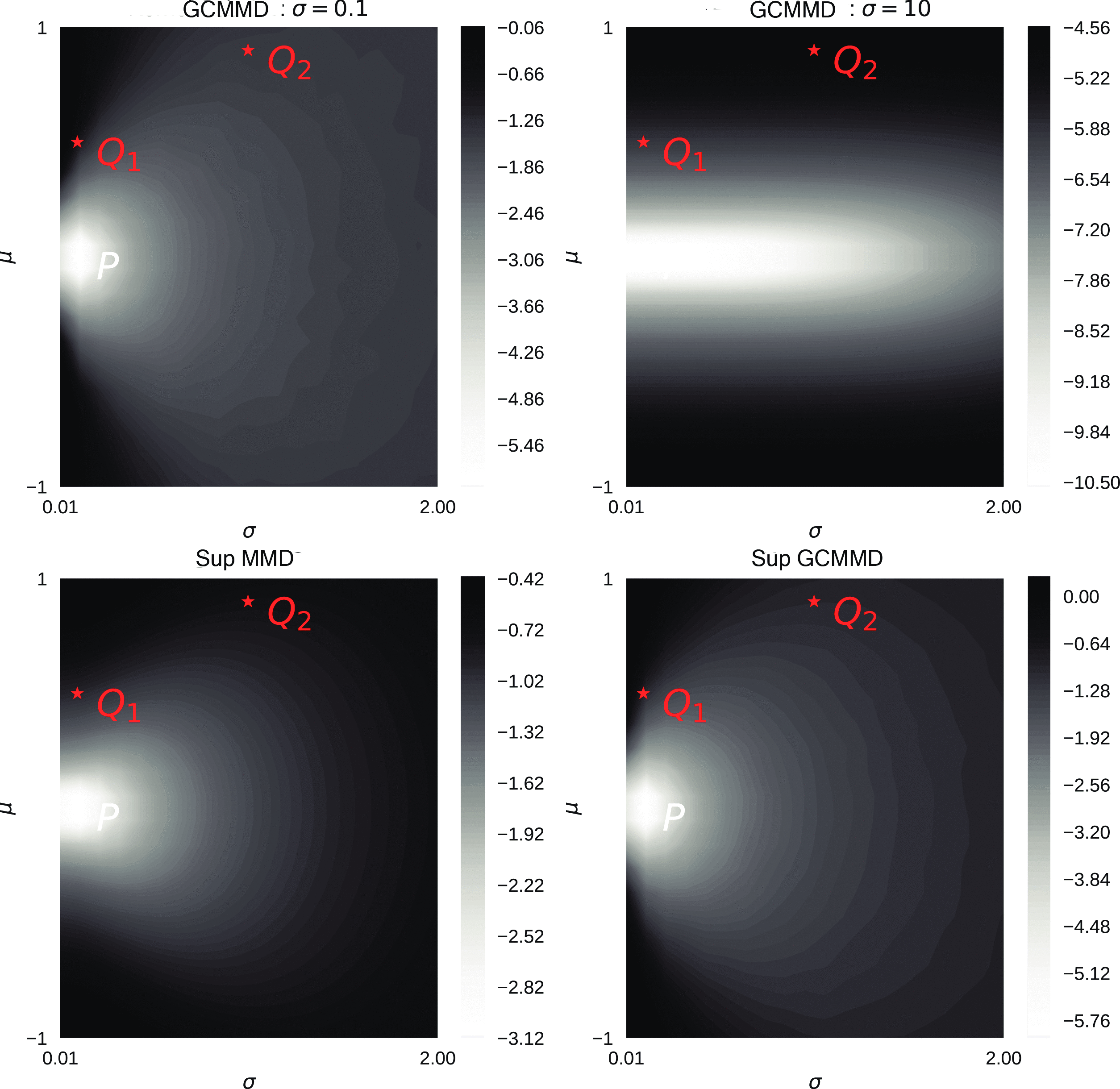
Figure 7 shows the behavior of the MMD, the Gradient-Constrained SMMD, and the Scaled MMD when comparing Gaussian distributions. We can see that and the Gradient-Constrained MMD behave similarly in this case, and that optimizing the and the Gradient-Constrained MMD is also similar. Optimizing the MMD would yield an essentially constant distance.
F.2 IGMs with Optimized Gradient-Constrained MMD loss
We implemented the estimator of 3 using the empirical mean estimator of , and sharing samples for . To handle the large but approximately low-rank matrix system, we used an incomplete Cholesky decomposition [43, Algorithm 5.12] to obtain such that . Then the Woodbury matrix identity allows an efficient evaluation:
Even though only a small is required for a good approximation, and the full matrices , , and need never be constructed, backpropagation through this procedure is slow and not especially GPU-friendly; training on CPU was faster. Thus we were only able to run the estimator on MNIST, and even that took days to conduct the optimization on powerful workstations.
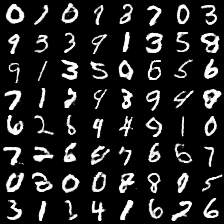
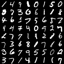
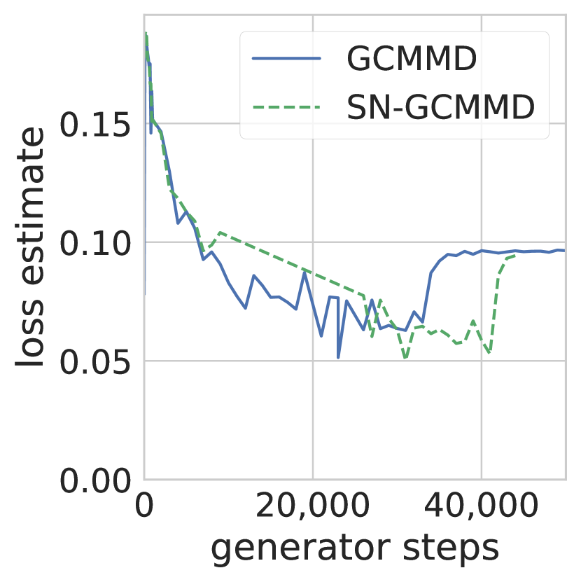
The learned models, however, were reasonable. Using a DCGAN architecture, batches of size 64, and a procedure that otherwise agreed with the setup of Section 4, samples with and without spectral normalization are shown in Figures 8(a) and 8(b). After the points in training shown, however, the same rank collapse as discussed in Section 4 occurred. Here it seems that spectral normalization may have delayed the collapse, but not prevented it. Figure 8(c) shows generator loss estimates through training, including the obvious peak at collapse; Figure 8(d) shows KID scores based on the MNIST-trained convnet representation [7], including comparable SMMD models for context. The fact that SMMD models converged somewhat faster than Gradient-Constrained MMD models here may be more related to properties of the estimator of 3 rather than the distances; more work would be needed to fully compare the behavior of the two distances.
F.3 Spectral normalization and Scaled MMD
Figure 9 shows the distribution of critic weight singular values, like Figure 2, at more layers. Figures 11 and 2 show results for the spectral normalization variants considered in the experiments. MMDGAN, with neither spectral normalization nor a gradient penalty, did surprisingly well in this case, though it fails badly in other situations.
Figure 9 compares the decay of singular values for layer of the critic’s network at both early and later stages of training in two cases: with or without the spectral parametrization. The model was trained on CelebA using SMMD. Figure 11 shows the evolution per iteration of Inception score, FID and KID for Sobolev-GAN, MMDGAN and variants of MMDGAN and WGAN using spectral normalization. It is often the case that this parametrization alone is not enough to achieve good results.

| IS | FID | KID | |
|---|---|---|---|
| Method | |||
| MMDGAN | 5.50.0 | 73.90.1 | 39.41.5 |
| SN-WGAN | 2.20.0 | 208.50.2 | 178.91.5 |
| SN-WGAN-GP | 2.50.0 | 154.30.2 | 125.30.9 |
| SN-Sobolev-GAN | 2.90.0 | 140.20.2 | 130.01.9 |
| SN-MMDGAN-GP | 4.60.1 | 96.80.4 | 59.51.4 |
| SN-MMDGAN-L2 | 7.10.1 | 31.90.2 | 21.70.9 |
| SN-MMDGAN | 6.90.1 | 31.50.2 | 21.71.0 |
| SN-MMDGAN-GP-L2 | 6.90.2 | 32.30.3 | 20.91.1 |
| SN-SMMDGAN | 7.30.1 | 25.00.3 | 16.62.0 |
F.4 Additional samples
Figures 12 and 13 give extra samples from the models.


