An exact solution for choosing the largest measurement from a sample drawn from an uniform distribution

Abstract

In “Recognizing the Maximum of a Sequence”, Gilbert and Mosteller analyze a full information game where n measurements from an uniform distribution are drawn and a player (knowing n) must decide at each draw whether or not to choose that draw. The goal is to maximize the probability of choosing the draw that corresponds to the maximum of the sample. In their calculations of the optimal strategy, the optimal probability and the asymptotic probability, they assume that after a draw x the probability that the next i numbers are all smaller than x is $x^{i}$; but this fails to recognize that continuing the game (not choosing a draw because it is lower than a cutoff and waiting for the next draw) conditions the distribution of the following i numbers such that their expected maximum is higher then i/(i+1). The problem is now redefined with each draw leading to a win, a false positive loss, a false negative loss and a continuation. An exact formula for these probabilities is deduced, both for the general case of n-1 different indifference numbers (assuming 0 as the last cutoff) and the particular case of the same indifference number for all cutoffs but the last. An approximation is found that preserves the main characteristics of the optimal solution (slow decay of win probability, quick decay of false positives and linear decay of false negatives). This new solution and the original Gilbert and Mosteller formula are compared against simulations, and their asymptotic behavior is studied.

1 Introduction

The class of problems known as “Secretary Problems” have been studied extensively in optimal stopping theory. The basic structure involves choosing the best (or second best) out of a sample of n elements (observed sequentially, one at a time) from a distribution, where it is possible to rank sequentially these elements; each rejection/acceptance decision is definitive and must be made immediately after each observation. The payoff might vary depending on the formulation of the problem.

In “Recognizing the Maximum of a Sequence”[1], Gilbert and Mosteller analyze a full information game where n measurements from an uniform distribution are drawn and a player (knowing n) must decide at each draw whether or not to choose that draw. The goal is to maximize the probability of choosing the draw that corresponds to the maximum of the sample. For that, at each round j one must choose whether to accept or reject the number $a_{j}$ based on a comparison with a decision number $k_{j}$. So, at round 1, $a_{1}\geqslant k_{1}$ with probability $1-k_{1}$. On the following rounds, the similar probabilities $a_{j}\geqslant k_{j}$ will be more complicated. For the last round, one should choose $k_{n}=0$ since there is only one number left.

It is a known result that the CDF, the PDF and the expected value of the maximum of n independent samples of an uniform distribution are $x^{n}$, $n\cdot x^{n-1}$ and n/(n+1), respectively. In their calculations of the optimal strategy, the optimal probability and the asymptotic probability, Gilbert and Mosteller assume that after a draw x the probability that the next i numbers are all smaller than x is $x^{i}$. From that, and considering the decision numbers to be indifference numbers (one should be indifferent between choosing a candidate if $a_{j}\geqslant k_{j}$ or continuing if $a_{j}<k_{j}$), Gilbert and Mosteller derive the probability of winning given an indifference number k and i remaining rounds as:

$$\sum_{j=1}^{i}\binom{i}{j}\frac{\cdot k^{i-j}\cdot(1-k)^{j}}{j}$$ (1)

Solving for k as an indifference number:

$$\sum_{j=1}^{i}\binom{i}{j}\frac{\cdot k^{i-j}\cdot(1-k)^{j}}{j}=k^{i}$$ (2)

These equations can be solved with Mathematica or Python (SymPy), and the solutions found are the same as those from the original paper, as Table 1 shows.

i	$k_{i}$
1	0.	0
2	0.	5
3	0.	68989795
4	0.	77584507
5	0.	82458958

i	$k_{i}$
50	0.	98377581
…	.	..
98	0.	99175674
99	0.	99184036
100	0.	99192231

Table 1: Indifference numbers $k_{i}$ as a function of the number of rounds remaining i, according to the formulas by Gilbert and Mosteller

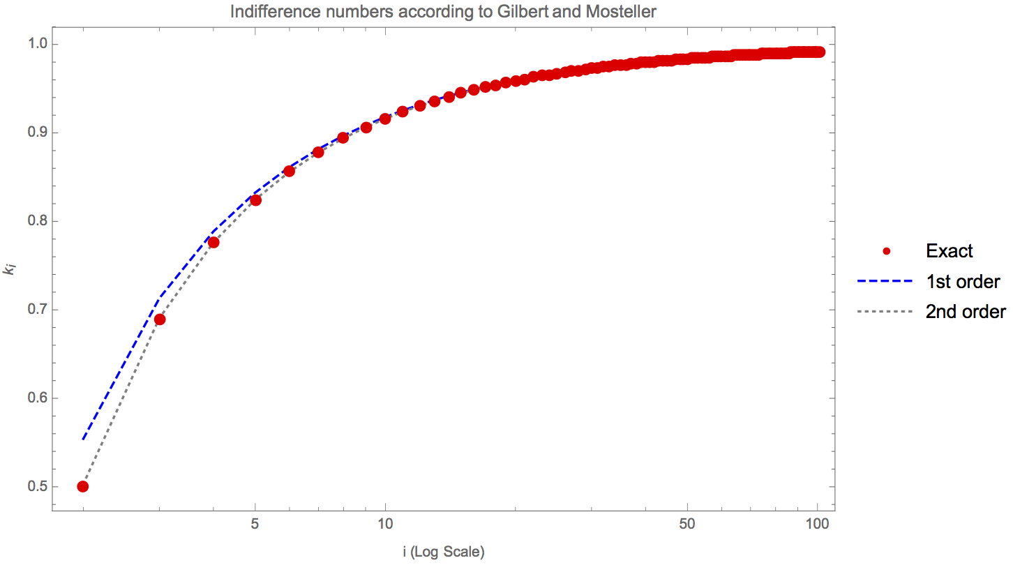
First and second order approximations were also derived, and Figure 1 shows that these approximations are good enough for any practical purpose.

Figure 1: Indifference numbers $k_{i}$ as a function of the number of rounds remaining i and their approximations (first and second order), according to the formulas by Gilbert and Mosteller

Gilbert and Mosteller derive the probability P(r+1) of winning at round r+1 in the particular case of monotone nonincreasing decision numbers $k_{1}\geqslant k_{2}\geqslant\ldots\geqslant k_{n-1}\geqslant k_{n}$ as:

$$P(r+1)=\sum_{j=1}^{r}\frac{k_{j}^{r}}{r\cdot(n-r)}-\sum_{j=1}^{r}\frac{k_{j}^{n}}{n\cdot(n-r)}-\frac{k_{r+1}^{n}}{n},1\leqslant r\leqslant n-1$$ (3)

$$P(1)=\frac{1}{n}-\frac{k_{1}^{n}}{n}$$ (4)

And the overall probability of winning as:

$$Pwin=\sum_{r=1}^{n}P(r)$$ (5)

For the decision numbers $k=\{k{}_{1},k_{2},0\}$ the probabilities at each round are $p=\{\frac{1}{3}-\frac{k_{1}^{3}}{3},\frac{k_{1}}{2}-\frac{k_{1}^{3}}{6}-\frac{k_{2}^{3}}{3},\frac{k_{1}^{2}}{2}-\frac{k_{1}^{3}}{3}+\frac{k_{2}^{2}}{2}-\frac{k_{2}^{3}}{3}\}$ and the overall probability is $Pwin=\frac{1}{3}+\frac{k_{1}}{2}+\frac{k_{1}^{2}}{2}-\frac{5k_{1}^{3}}{6}+\frac{k_{2}^{2}}{2}-\frac{2k_{2}^{3}}{3}$.

Substituting the values from Table 1 with $k_{i}\rightarrow k_{n-j+1}$ (for n=3, the indifference number $k_{1}$ used in the first round is $k_{3}$ from Table 1), the overall win probabilities can be calculated.

Calculating the probabilities up to n=100, they agree with the original paper (that went only to n=50), as Table 2 shows.

n	Pwin
1	1.	0
2	0.	75
3	0.	684293
4	0.	655396
5	0.	639194

n	Pwin
10	0.	608699
50	0.	585725
98	0.	582993
99	0.	582964
100	0.	582936

Table 2: Overall win probabilities (using the substitution $k_{i}\rightarrow k_{n-j+1}$ where $k_{i}$ is an indifference number and $k_{n-j+1}$ is a decision number) as a function of the number of rounds n, according to the formulas by Gilbert and Mosteller

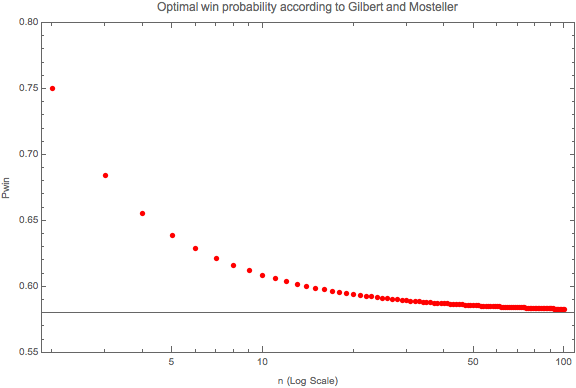
Figure 2 shows Pwin for n up to 100, with 0.58 a likely estimate for the limit for $n\rightarrow\infty$.

Figure 2: Overall win probabilities (using the substitution $k_{i}\rightarrow k_{n-j+1}$ where $k_{i}$ is an indifference number and $k_{n-j+1}$ is a decision number) as a function of the number of rounds n, according to the formulas by Gilbert and Mosteller

It is worth to compare these results with a naive strategy of choosing decreasing decision numbers such that:

$$k_{n,j}=1-\frac{1}{n-j+1}$$ (6)

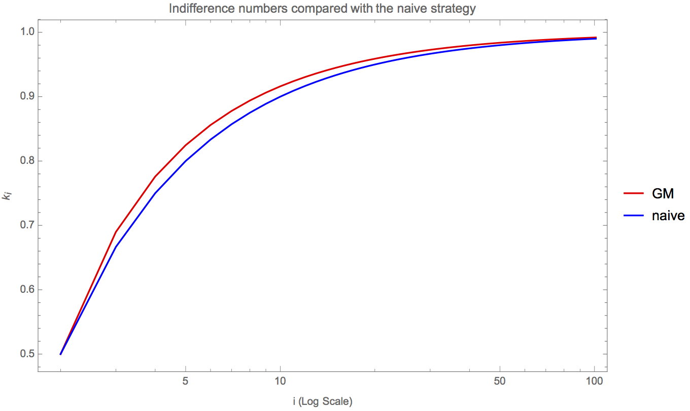
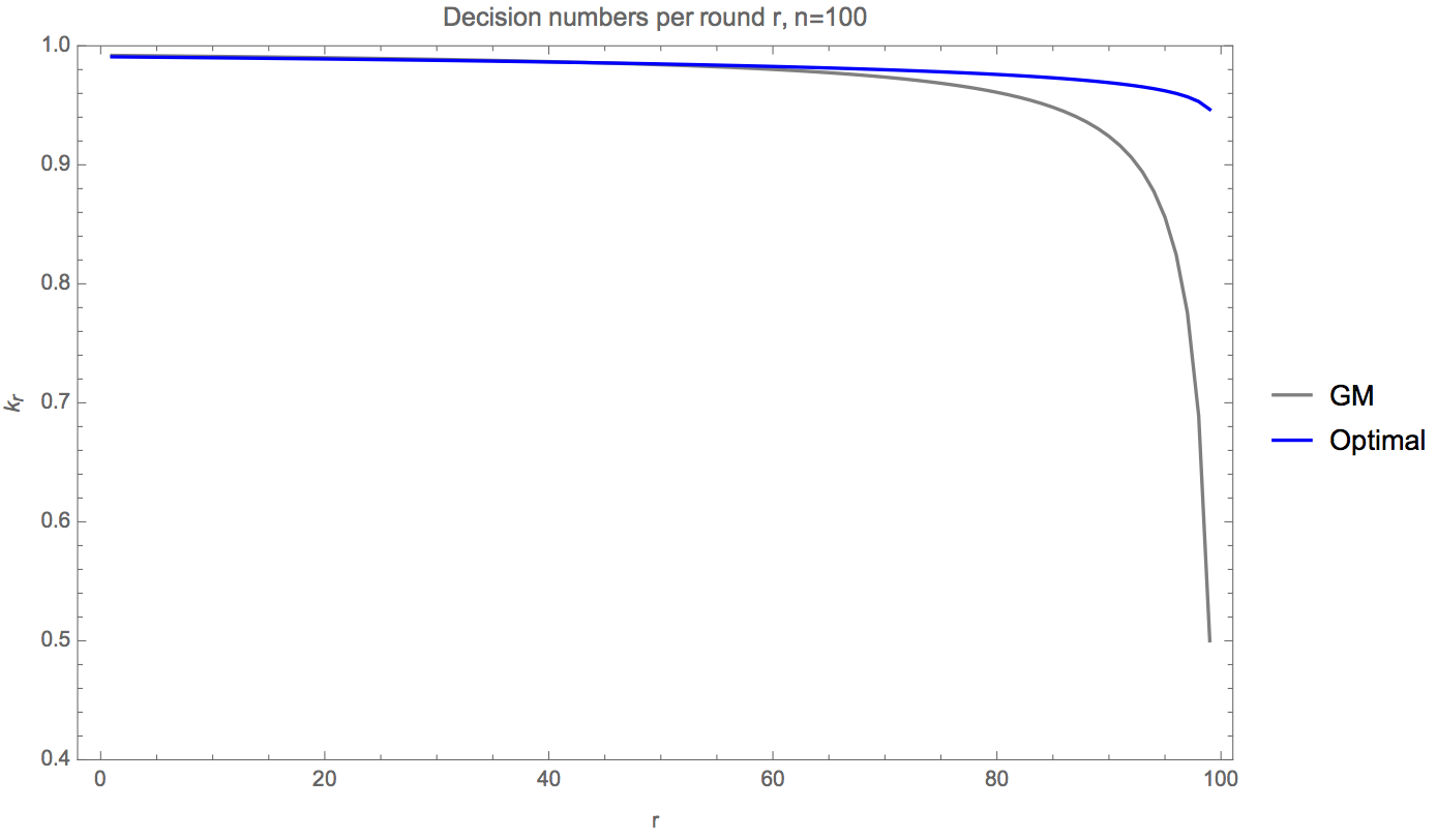
This strategy also has $k_{n}=0$, and for 2<n<100 the values are lower than those in Gilbert and Mosteller (Figure 3).

Figure 3: Indifference numbers $k_{i}$ as a function of the number of rounds remaining i according to the formulas by Gilbert and Mosteller and according to the naive strategy

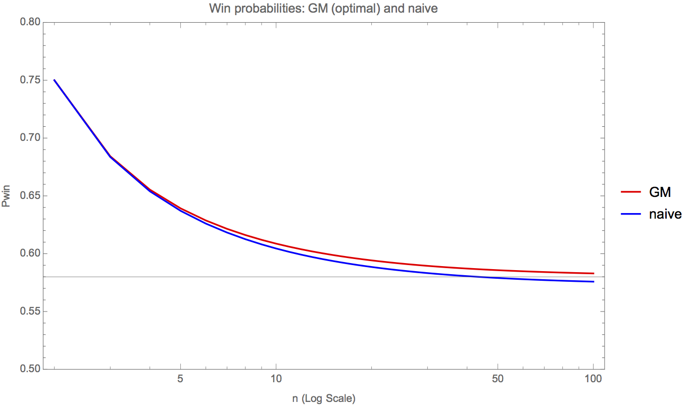
And, as expected, has a slightly lower overall win probability than the (optimal) Gilbert and Mosteller probability (Figure 4).

Figure 4: Overall win probabilities as a function of the number of rounds n, according to the formulas by Gilbert and Mosteller and according to the naive strategy

The cases of a single decision number k for all rounds and and a single decision number k for t rounds followed by 0 in the last n-t rounds are also studied by Gilbert and Mosteller; the asymptotic probability in the first case was calculated by Gilbert and Mosteller to be:

$$Pwinklim=\sum_{i=1}^{\infty}\frac{e^{-\mu}\cdot\mu^{i}}{i!\cdot i}$$ (7)

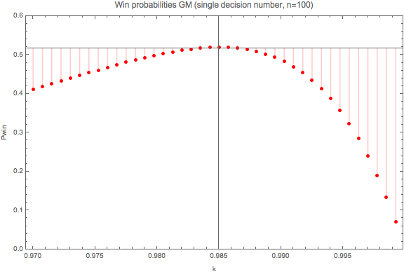
And with $\mu\thickapprox 1.503$ one finds $Pwinklim\thickapprox 0.51735$. For large n this maximum seems to require $k=1-\frac{1.5}{n}$, as seen for n=100 in Figure 5 and similar plots for even larger n (not shown).

Figure 5: Overall win probabilities as a function of the value of k for a single decision number (with n=100), according to the formulas by Gilbert and Mosteller

In the second case, for n=100 and integer values for t one finds the optimal values t=65, k=0.9883 and Pwin=0.566684, not far from the values provided by Gilbert and Mosteller.

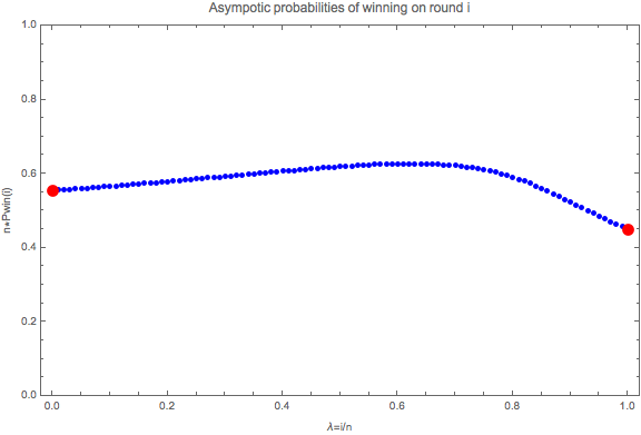
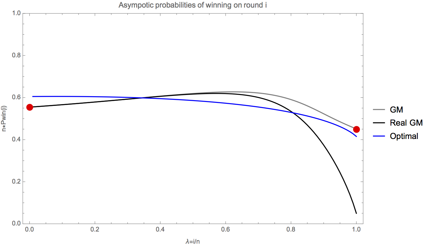
And finally Gilbert and Mosteller present results similar to Figure 6 as the asymptotic probability of winning at round i, including the $1-e^{-c}$ and $e^{-c}$ extremes (red points).

Figure 6: Win probabilities per round for the optimal choices with n=100 according to the formulas by Gilbert and Mosteller

With the Gilbert and Mosteller paper summarized and the formulas implemented, it’s time to examine the problem again, but from a different angle.

2 Visualization of the problem

For n=2, the possible values of the draws $\{a_{1},a_{2}\}$ fill an unit square; the region where $a_{1}\geqslant a_{2}$ is the one below the diagonal with origin {0,0} and endpoint {1,1}, and the region where $a_{1}<a_{2}$ is the one above the same diagonal. Given a choice for $k_{1}$, the possibilities can be represented by Figure 7:

Figure 7: Possibilities for n=2

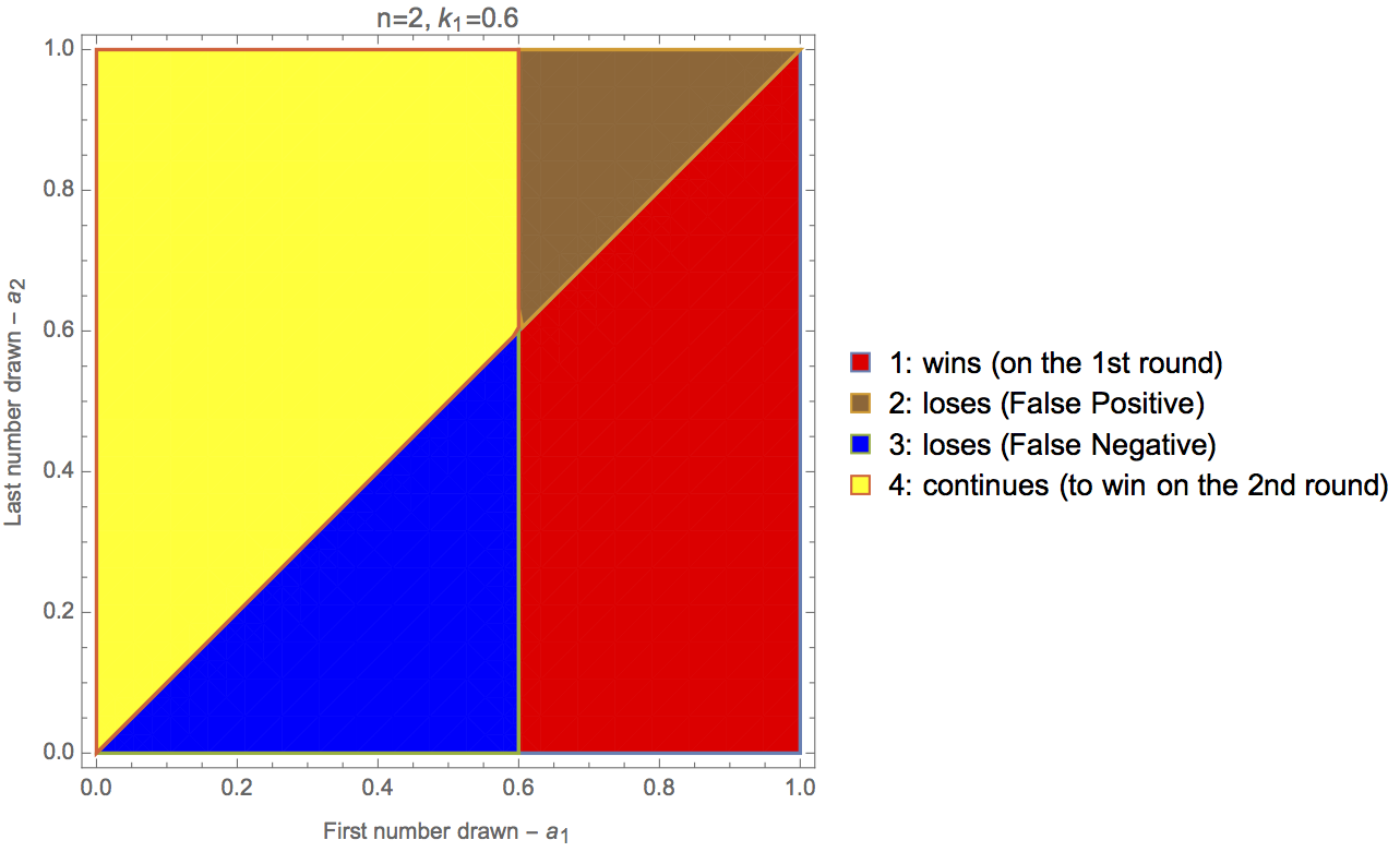
There are 3 ways for the game to end at round 1:

• Win ($a_{1}\geqslant k_{1}\land a_{1}=\max(a_{j})$) - the red area in Figure 7

• Loss due to a False Positive ($a_{1}\geqslant k_{1}\land a_{1}\neq\max(a_{j})$) - the brown area in Figure 7

• Loss due to a False Negative ($a_{1}<k_{1}\land a_{1}=\max(a_{j})$) - the blue area in Figure 7

If the game has not ended at round 1, it means that it will end at round 2 with:

• Win ($a_{2}\geqslant k_{2}=0\land a_{2}=\max(a_{j})\land a{}_{1}<k_{1}\land a_{1}\neq\max(a_{j})$) - the yellow area in Figure 7

Which for the particular case of n=2 and $k_{2}=0$ can be written as:

• Win ($a_{1}<k_{1}\land a_{1}\neq\max(a_{j})$)

The optimal strategy (already considering $k_{2}=0$) is reached by choosing $k_{1}$ such that the sum of the two win probabilities (at rounds 1 and 2) is maximal.

Before solving that, it is important to look at the n=3 case.

For n=3, the possible values of the draws $\{a_{1},a_{2},a_{3}\}$ fill an unit cube; the region where $a_{1}=\max(a_{j})$ is the yangma shown in Figure 8.

Figure 8: The region where $a_{1}=\max(a_{j})$ for n=3

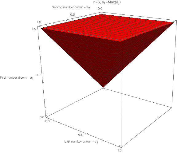
There are 3 ways for the game to end at round 1:

• Win ($a_{1}\geqslant k_{1}\land a_{1}=\max(a_{j})$) - the red region in Figure 9

• Loss due to a False Positive ($a_{1}\geqslant k_{1}\land a_{1}\neq\max(a_{j})$) - the brown region in Figure 9 (rotated view)

• Loss due to a False Negative ($a_{1}<k_{1}\land a_{1}=\max(a_{j})$) - the blue region in Figure 9

Figure 9: Regions where the game ends in round 1 for n=3; the brown region’s view was rotated

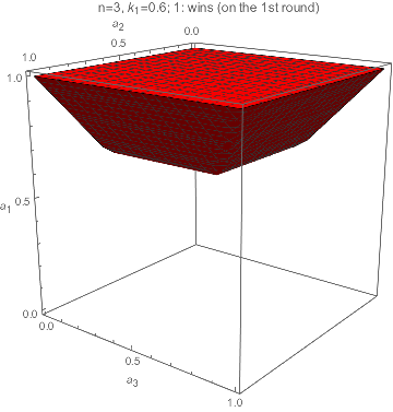
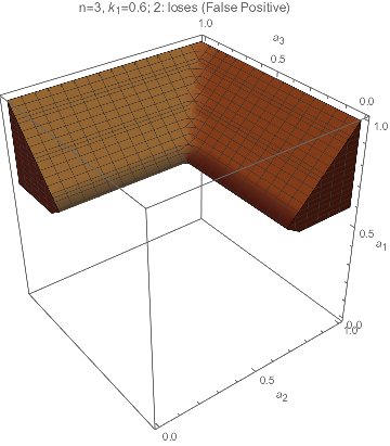
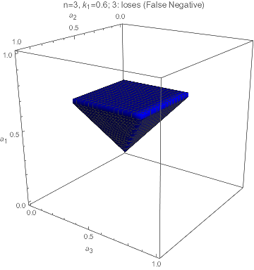
If the game has not ended at round 1, it means that it will continue to round 2 in this situation:

• Continue ($a_{1}<k_{1}\land a_{1}\neq\max(a_{j})$) - the yellow region in Figure 10; it is very important to notice that there’s a piece missing (corresponding to the false negative of round 1, the 3rd region of Figure 9), and $\{a_{2},a_{3}\}$ is not similar to the n=2 case anymore, as Figure 11 indicates.

Figure 10: Region where the game continues from round 1 to round 2 for n=3

Figure 11: A cut from Figure 10, showing how round 2 for n=3 is not equal to n=2

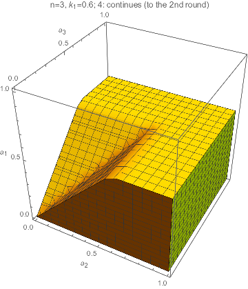
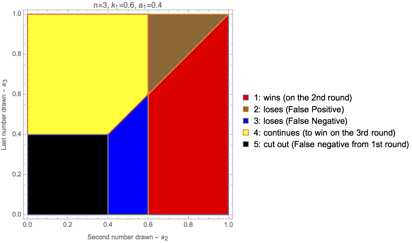
There are 3 ways for the game to end at round 2:

• Win ($a_{2}\geqslant k_{2}\land a_{2}=\max(a_{j})\land a_{1}<k_{1}\land a_{1}\neq\max(a_{j})$) - the red area in Figure 11 and the red region in Figure 12

• Loss due to a False Positive ($a_{2}\geqslant k_{2}\land a_{2}\neq\max(a_{j})\land a_{1}<k_{1}\land a_{1}\neq\max(a_{j})$) - the brown area in Figure 11 and the brownd region in Figure 12

• Loss due to a False Negative ($a_{2}<k_{2}\land a_{2}=\max(a_{j})\land a_{1}<k_{1}\land a_{1}\neq\max(a_{j})$) - the blue area in Figure 11 and the blue region in Figure 12

Figure 12: Regions where the game ends in round 2 for n=3; the brown region’s view was rotated

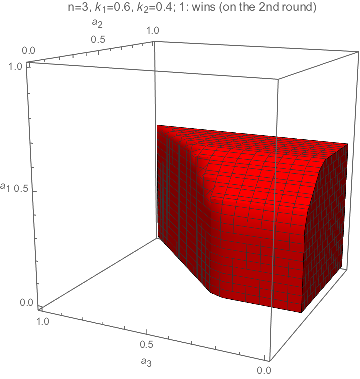
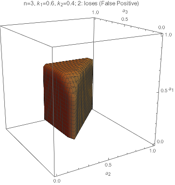
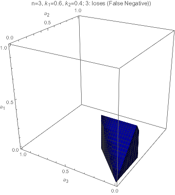
If the game has not ended at round 2, it means that it will end at round 3 with:

• Win ($a_{3}\geqslant k_{3}=0\land a_{3}=\max(a_{j})\land a_{2}<k_{2}\land a_{2}\neq\max(a_{j})\land a_{1}<k_{1}\land a_{1}\neq\max(a_{j})$) - the yellow area in Figure 11 and the the yellow region in Figure 13

Figure 13: Region where the game continues from round 2 to round 3 for n=3

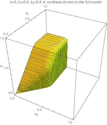
Which for the particular case of n=3 and $k_{3}=0$ can be written as:

• Win ($a_{2}<k_{2}\land a_{2}\neq\max(a_{j})\land a_{1}<k_{1}\land a_{1}\neq\max(a_{j})$)

It is worth noticing that at each round the region where the game continues from one round to the next becomes narrower at the “bottom” and more “top-heavy”; it means that the expected value of the maximum of a game with n draws after r rounds should be increasing when compared with the same game for n-r draws at the first round, as the false negatives accumulate.

3 Solving for small n through integration

In the same way that Mathematica can plot the areas and regions in the previous section, it can integrate the areas of the unit square and the regions of the unit cube; it will also integrate the regions of the unit hypercubes for values of n higher than 3 (but not much higher).

The process is automated by:

• Defining a function that, given n, conditions and assumptions, generates the variables table and the n uniform distributions to calculate Assuming[assumptions,Probability[conditions,distributions]]

• Defining a function that receives as input:

  • the number of draws n

  • the round of interest r (implies that in previous rounds $((a_{i}<k_{i})\land(a_{i}\neq\max(a_{j})))\forall i<r$)

  • the array of decision numbers k (symbolic or numeric)

  • the flag ak for use of the comparison between $a_{r}$ and $k_{r}$ (True or False)

  • the flag amax for use of the comparison between $a_{r}$ and $\max(a_{j})$ (True or False)

  • the function fak for the comparison between $a_{r}$ and $k_{r}$ (GreaterEqual or Less)

  • the function famax for the comparison between $a_{r}$ and $\max(a_{j})$ (GreaterEqual or Less)

  • the logical connection between the conditions coming from the previous rounds and the comparisons for the round r (And or Conditioned)

For n=2, we have the following probabilities (Table 3):

r	W	L (FP)	L (FN)	C
1	$\frac{1}{2}-\frac{k_{1}^{2}}{2}$	$\frac{1}{2}-k_{1}+\frac{k_{1}^{2}}{2}$	$\frac{k_{1}^{2}}{2}$	$k_{1}-\frac{k_{1}^{2}}{2}$
2	$k_{1}-\frac{k_{1}^{2}}{2}$	0	0	0

Table 3: Probabilities for n=2

The probabilities from the Gilbert and Mosteller paper for wins in rounds 1 and 2 are $\frac{1}{2}-\frac{k_{1}^{2}}{2}$ and $k_{1}-\frac{k_{1}^{2}}{2}$, respectively, so these calculations match and the optimal $k_{1}=\frac{1}{2}$ for a total probability of $\frac{3}{4}$, evenly distributed between rounds 1 and 2.

For n=3, and assuming nonincreasing decision numbers, we have the following probabilities (Table 4):

r	W	L (FP)	L (FN)	C
1	$\frac{1}{3}-\frac{k_{1}^{3}}{3}$	$\frac{2}{3}-k_{1}+\frac{k_{1}^{3}}{3}$	$\frac{k_{1}^{3}}{3}$	$k_{1}-\frac{k_{1}^{3}}{3}$
2	$\frac{k_{1}}{2}-\frac{k_{1}^{3}}{6}-\frac{k_{2}^{3}}{3}$	$\frac{k_{1}}{2}-\frac{k_{1}^{3}}{6}-k_{1}k_{2}+\frac{k_{1}^{2}k_{2}}{2}+\frac{k_{2}^{3}}{6}$	$\frac{k_{2}^{3}}{3}$	$k_{1}k_{2}-\frac{k_{1}^{2}k_{2}}{2}-\frac{k_{2}^{3}}{6}$
3	$k_{1}k_{2}-\frac{k_{1}^{2}k_{2}}{2}-\frac{k_{2}^{3}}{6}$	0	0	0

Table 4: Probabilities for n=3

The probabilities from the Gilbert and Mosteller paper for wins in rounds 1, 2 and 3 are $\frac{1}{3}-\frac{k_{1}^{3}}{3}$, $\frac{k_{1}}{2}-\frac{k_{1}^{3}}{6}-\frac{k_{2}^{3}}{3}$ and $\frac{k_{1}^{2}}{2}-\frac{k_{1}^{3}}{3}+\frac{k_{2}^{2}}{2}-\frac{k_{2}^{3}}{3}$, respectively; these calculations match on the first and second round, but not on the last. Why? The conditions used on the calculations for round 3 in Table 4 are: $a_{3}\geq 0\land a_{3}\geq\max\left(a_{1},a_{2},a_{3}\right)\land a_{1}<k_{1}\land a_{2}<k_{2}\land\max\left(a_{1},a_{2}\right)<\max\left(a_{1},a_{2},a_{3}\right)$, while the result from Gilbert and Mosteller assumes the sum of the probabilities with conditions $a_{3}\geq 0\land a_{3}\geq\max\left(a_{1},a_{2},a_{3}\right)\land a_{1}<k_{1}\land\max\left(a_{1},a_{2}\right)<\max\left(a_{1},a_{2},a_{3}\right)$ and $a_{3}\geq 0\land a_{3}\geq\max\left(a_{1},a_{2},a_{3}\right)\land a_{2}<k_{2}\land\max\left(a_{1},a_{2}\right)<\max\left(a_{1},a_{2},a_{3}\right)$; that’s why there are no cross terms in Gilbert and Mosteller. But as seen on the previous section, the false negatives change the distribution of the following rounds, and one cannot simply add the probabilities.

To optimize the n=3 case one needs to maximize the sum of the Win column in Table 4:

$$\frac{1}{3}+\frac{k_{1}}{2}-\frac{k_{1}^{3}}{2}+k_{1}k_{2}-\frac{k_{1}^{2}k_{2}}{2}-\frac{k_{2}^{3}}{2}$$ (8)

The results are:

• $k_{1}\to 0.672608$

• $k_{2}\to 0.545532$ (not 0.5, the optimal k for n=2 is not optimal here, since the maximum of the round 2 region is higher than the maximum of the unit square)

• $pwin\to 0.679846$

Remembering that Gilbert and Mosteller had:

• $k_{1}\to 0.689898$

• $k_{2}\to 0.5$

• $pwin\to 0.684293$

But substituting the Gilbert and Mosteller values for the decision numbers in Equation 8 the result is a probability of 0.67785.

This disagreement will be tested with simulations in a further section.

4 Generalization of the formulas

The table for n=4 is shown below (Table 5). From it some patterns can be distinguished. It will be convenient to assume $PCon(n,r=0)=1$.

r	W	L (FP)	L (FN)	C
1	$\frac{1}{4}-\frac{k_{1}^{4}}{4}$	$\frac{3}{4}-k_{1}+\frac{k_{1}^{4}}{4}$	$\frac{k_{1}^{4}}{4}$	$k_{1}-\frac{k_{1}^{4}}{4}$
2	$\frac{k_{1}}{3}-\frac{k_{1}^{4}}{12}-\frac{k_{2}^{4}}{4}$	$\frac{2k_{1}}{3}-\frac{k_{1}^{4}}{6}-k_{1}k_{2}+\frac{k_{1}^{3}k_{2}}{3}+\frac{k_{2}^{4}}{6}$	$\frac{k_{2}^{4}}{4}$	$k_{1}k_{2}-\frac{k_{1}^{3}k_{2}}{3}-\frac{k_{2}^{4}}{6}$
3	$\frac{k_{1}k_{2}}{2}-\frac{k_{1}^{3}k_{2}}{6}-\frac{k_{2}^{4}}{12}-\frac{k_{3}^{4}}{4}$	$\frac{k_{1}k_{2}}{2}-\frac{k_{1}^{3}k_{2}}{6}-\frac{k_{2}^{4}}{12}-k_{1}k_{2}k_{3}+\frac{k_{1}^{2}k_{2}k_{3}}{2}+\frac{k_{2}^{3}k_{3}}{6}+\frac{k_{3}^{4}}{12}$	$\frac{k_{3}^{4}}{4}$	$k_{1}k_{2}k_{3}-\frac{k_{1}^{2}k_{2}k_{3}}{2}-\frac{k_{2}^{3}k_{3}}{6}-\frac{k_{3}^{4}}{12}$
4	$k_{1}k_{2}k_{3}-\frac{k_{1}^{2}k_{2}k_{3}}{2}-\frac{k_{2}^{3}k_{3}}{6}-\frac{k_{3}^{4}}{12}$	0	0	0

Table 5: Probabilities for n=4

The false negatives are unaffected by the previous rounds, depending only on the decision number for their round:

$$PFN(n,r)=\frac{k_{r}^{n}}{n},1\leqslant r\leqslant n$$ (9)

As expected, the sum of the Win and False Negative probabilities, divided (conditioned) on the Continue probability of the previous round, is equal to 1/(n-r+1):

$$PW(n,r)=\frac{PC(n,r-1)}{(n-r+1)}-PFN(n,r),1\leqslant r\leqslant n$$ (10)

The first r terms of the False Positive probability is equal to the difference between the Continue probability of the previous round and the sum of the Win probability and the False Negative probability of the same round. The other terms are equal to the terms of the Continue probability of the same round, but the the opposite sign. This is expected, but it helps to save space, as this is the longest formula:

$$PFP(n,r)=(PC(n,r-1)-(PW(n,r)+PFN(n,r)))-PC(n,r)$$ (11)

Rewriting Table 5, we have Table 6, which will enable the tables for n=5 and 6 to be written more easily, as what matters is finding the formula for PC(n,r):

r	n-r+1	W	L (FP)	L (FN)	C
0	-	-	-	-	1
1	4	$\frac{PC(4,0)}{4}-PFN(4,1)$	$(PC(4,0)-(PW(4,1)+PFN(4,1)))-PC(4,1)$	$\frac{k_{1}^{4}}{4}$	$k_{1}-\frac{k_{1}^{4}}{4}$
2	3	$\frac{PC(4,1)}{3}-PFN(4,2)$	$(PC(4,1)-(PW(4,2)+PFN(4,2)))-PC(4,2)$	$\frac{k_{2}^{4}}{4}$	$k_{1}k_{2}-\frac{k_{1}^{3}k_{2}}{3}-\frac{k_{2}^{4}}{6}$
3	2	$\frac{PC(4,2)}{2}-PFN(4,3)$	$(PC(4,2)-(PW(4,3)+PFN(4,3)))-PC(4,3)$	$\frac{k_{3}^{4}}{4}$	$k_{1}k_{2}k_{3}-\frac{k_{1}^{2}k_{2}k_{3}}{2}-\frac{k_{2}^{3}k_{3}}{6}-\frac{k_{3}^{4}}{12}$
4	1	$\frac{PC(4,3)}{1}-0$	0	0	0

Table 6: Probabilities for n=4 (simplified)

r	n-r+1	L (FN)	C
0	-	-	1
1	5	$\frac{k_{1}^{5}}{5}$	$k_{1}-\frac{k_{1}^{5}}{5}$
2	4	$\frac{k_{2}^{5}}{5}$	$k_{1}k_{2}-\frac{k_{1}^{4}k_{2}}{4}-\frac{3k_{2}^{5}}{20}$
3	3	$\frac{k_{3}^{5}}{5}$	$k_{1}k_{2}k_{3}-\frac{k_{1}^{3}k_{2}k_{3}}{3}-\frac{k_{2}^{4}k_{3}}{6}-\frac{k_{3}^{5}}{10}$
4	2	$\frac{k_{4}^{5}}{5}$	$k_{1}k_{2}k_{3}k_{4}-\frac{k_{1}^{2}k_{2}k_{3}k_{4}}{2}-\frac{k_{2}^{3}k_{3}k_{4}}{6}-\frac{k_{3}^{4}k_{4}}{12}-\frac{k_{4}^{5}}{20}$
5	1	0	0

Table 7: Continuation probabilities for n=5

r	n-r+1	L (FN)	C
0	-	-	1
1	6	$\frac{k_{1}^{6}}{6}$	$k_{1}-\frac{k_{1}^{6}}{6}$
2	5	$\frac{k_{2}^{6}}{6}$	$k_{1}k_{2}-\frac{k_{1}^{5}k_{2}}{5}-\frac{2k_{2}^{6}}{15}$
3	4	$\frac{k_{3}^{6}}{6}$	$k_{1}k_{2}k_{3}-\frac{k_{1}^{4}k_{2}k_{3}}{4}-\frac{3k_{2}^{5}k_{3}}{20}-\frac{k_{3}^{6}}{10}$
4	3	$\frac{k_{4}^{6}}{6}$	$k_{1}k_{2}k_{3}k_{4}-\frac{k_{1}^{3}k_{2}k_{3}k_{4}}{3}-\frac{k_{2}^{4}k_{3}k_{4}}{6}-\frac{k_{3}^{5}k_{4}}{10}-\frac{k_{4}^{6}}{15}$
5	2	$\frac{k_{5}^{6}}{6}$	$k_{1}k_{2}k_{3}k_{4}k_{5}-\frac{k_{1}^{2}k_{2}k_{3}k_{4}k_{5}}{2}-\frac{k_{2}^{3}k_{3}k_{4}k_{5}}{6}-\frac{k_{3}^{4}k_{4}k_{5}}{12}-\frac{k_{4}^{5}k_{5}}{20}-\frac{k_{5}^{6}}{30}$
6	1	0	0

Table 8: Continuation probabilities for n=6

The formula for PC can be decomposed as:

$$PC(n,r)=\prod_{j=1}^{r}k_{j}-\sum_{i=1}^{r}\left(g(i,n,r)\prod_{j=1}^{r}k_{j}^{f(i,j,n,r)}\right)\ ,\ \sum_{j=1}^{r}f(i,j,n,r)=n\forall i,r$$ (12)

With f(i,j,n,r) and g(i,n,r) highlighted on Tables 9 and 10, respectively:

r=1	j
i	1
1	6

r=2	j
i	1	2
1	5	1
2	0	6

r=3	j
i	1	2	3
1	4	1	1
2	0	5	1
3	0	0	6

r=4	j
i	1	2	3	4
1	3	1	1	1
2	0	4	1	1
3	0	0	5	1
4	0	0	0	6

r=5	j
i	1	2	3	4	5
1	2	1	1	1	1
2	0	3	1	1	1
3	0	0	4	1	1
4	0	0	0	5	1
5	0	0	0	0	6

Table 9: f(i,j) for n=6

$$f(i,j,n,r)=\begin{cases}n-r+i&i=j\\ 1&i<j\\ 0&i>j\end{cases}$$ (13)

r=1
i	n-r+i	g(i)
1	6	$\frac{1}{6}=\frac{5}{5\cdot 6}$

r=2
i	n-r+i	g(i)
1	5	$\frac{1}{5}=\frac{4}{4\cdot 5}$
2	6	$\frac{2}{15}=\frac{4}{5\cdot 6}$

r=3
i	n-r+i	g(i)
1	4	$\frac{1}{4}=\frac{3}{3\cdot 4}$
2	5	$\frac{3}{20}=\frac{3}{4\cdot 5}$
3	6	$\frac{1}{10}=\frac{3}{5\cdot 6}$

r=4
i	n-r+i	g(i)
1	3	$\frac{1}{3}=\frac{2}{2\cdot 3}$
2	4	$\frac{1}{6}=\frac{2}{3\cdot 4}$
3	5	$\frac{1}{10}=\frac{2}{4\cdot 5}$
4	6	$\frac{1}{15}=\frac{2}{5\cdot 6}$

r=5
i	n-r+i	g(i)
1	2	$\frac{1}{3}=\frac{1}{1\cdot 2}$
2	3	$\frac{1}{6}=\frac{1}{2\cdot 3}$
3	4	$\frac{1}{12}=\frac{1}{3\cdot 4}$
4	5	$\frac{1}{20}=\frac{1}{4\cdot 5}$
5	6	$\frac{1}{30}=\frac{1}{5\cdot 6}$

Table 10: g(i) for n=6

$$g(i,n,r)=\frac{(n-r)}{(n-r+i-1)(n-r+i)}$$ (14)

And so the final formula for PC is:

$$PC(n,r)=\prod_{j=1}^{r}k_{j}-\sum_{i=1}^{r}\left(\frac{(n-r)}{(n-r+i-1)(n-r+i)}\prod_{j=1}^{r}k_{j}^{f(i,j,n,r)}\right)\ ,\ f(i,j,n,r)=\begin{cases}n-r+i&i=j\\ 1&i<j\\ 0&i>j\end{cases}$$ (15)

And therefore the formula for PW(n,r) is:

$$PW(n,r)=\frac{PC(n,r-1)}{(n-r+1)}-PFN(n,r)$$

$$PW(n,r)=\frac{1}{(n-r+1)}\prod_{j=1}^{r-1}k_{j}-\sum_{i=1}^{r-1}\left(\frac{1}{(n-r+i-1)(n-r+i)}\prod_{j=1}^{r-1}k_{j}^{f(i,j,n,r)}\right)-\frac{k_{r}^{n}}{n}\ ,\ f(i,j,n,r)=\begin{cases}n-r+i&i=j\\ 1&i<j\\ 0&i>j\end{cases}$$ (16)

The formula for PFP is not going to be written explicitly, but the definition of 11 will be used.

The formula for PW(n) is:

$$PW(n)=\sum_{r=1}^{n}PW(n,r)$$ (17)

This is the function that will be maximized by choosing the decision numbers $k_{j}$.

5 The formula for identical decision numbers

One can replace all indexed ks in the formulas above (keeping the last k as zero), but it is interesting to observe that the processing time for the integration involved in the probabilities calculation with n going from 2 to 6 fell from 4728 seconds for the general case to 84 seconds for the particular case.

Table shows PW for n going from 2 to 6:

n=2
r	PW
1	$\frac{1}{2}-\frac{k^{2}}{2}$
2	$k-\frac{k^{2}}{2}$

n=3
r	PW
1	$\frac{1}{3}-\frac{k^{3}}{3}$
2	$\frac{k}{2}-\frac{k^{3}}{2}$
3	$k^{2}-\frac{2k^{3}}{3}$

n=4
r	PW
1	$\frac{1}{4}-\frac{k^{4}}{4}$
2	$\frac{k}{3}-\frac{k^{4}}{3}$
3	$\frac{k^{2}}{2}-\frac{k^{4}}{2}$
4	$k^{3}-\frac{3k^{4}}{4}$

n=5
r	PW
1	$\frac{1}{5}-\frac{k^{5}}{5}$
2	$\frac{k}{4}-\frac{k^{5}}{4}$
3	$\frac{k^{2}}{3}-\frac{k^{5}}{3}$
4	$\frac{k^{3}}{2}-\frac{k^{5}}{2}$
5	$k^{4}-\frac{4k^{5}}{5}$

n=6
r	PW
1	$\frac{1}{6}-\frac{k^{6}}{6}$
2	$\frac{k}{5}-\frac{k^{6}}{5}$
3	$\frac{k^{2}}{4}-\frac{k^{6}}{4}$
4	$\frac{k^{3}}{3}-\frac{k^{6}}{3}$
5	$\frac{k^{4}}{2}-\frac{k^{6}}{2}$
6	$k^{5}-\frac{5k^{6}}{6}$

Table 11: PW for identical decision numbers {k,k,…,k,0}

The formula for PW(n,r) in this case is:

$$PW_{k}(n,r)=\frac{k^{r-1}}{n-r+1}-\frac{k^{n}}{n-r+1}+\begin{cases}0&1\leqslant r\leqslant n-1\\ \frac{k^{n}}{n}&r=n\end{cases}$$ (18)

Which can be simplified as:

$$PW_{k}(n,r)=k^{n}\left(\frac{1}{(n-r+1)k^{n-r+1}}-\frac{1}{(n-r+1)}+\begin{cases}0&1\leqslant r\leqslant n-1\\ \frac{1}{n}&r=n\end{cases}\right)$$ (19)

The formula for the overall probability is:

$$PW_{k}(n)=k^{n}\left(\sum_{r=1}^{n}\left(\frac{1}{(n-r+1)k^{n-r+1}}-\frac{1}{(n-r+1)}\right)+\frac{1}{n}\right)$$ (20)

Which can be broken into two sums:

$$PW_{k}(n)=k^{n}\left(\sum_{r=1}^{n}\left(\frac{1}{(n-r+1)k^{n-r+1}}\right)-\sum_{r=1}^{n}\left(\frac{1}{(n-r+1)}\right)+\frac{1}{n}\right)$$ (21)

And expressed with special functions as:

$$PW_{k}(n)=k^{n}\left(\sum_{r=1}^{n}\left(\frac{1}{(n-r+1)k^{n-r+1}}\right)-(\psi^{(0)}(n)+\gamma)\right)$$ (22)

Where $\psi^{(0)}(n)$ is the Digamma function and $\gamma$ is the Euler Gamma constant (see Table ).

n	$\psi^{(0)}(n)+\gamma$
2	1
3	$\frac{3}{2}$
4	$\frac{11}{6}$
5	$\frac{25}{12}$
6	$\frac{137}{60}$

Table 12: Values of Digamma(n)+EulerGamma

6 The optimal values

It is considerably easier to find the optimal values in the identical decision numbers case; in 30 seconds all the values for n going from 2 to 100 can be calculated. In 9 seconds the values for n=10000 can be calculated.

n	$1-\frac{1.5}{n}$		k		$PW_{k}(n)$
2	0.	25	0.	5	0.	75
3	0.	5	0.	622839	0.	670256
4	0.	625	0.	697839	0.	631163
5	0.	7	0.	748138	0.	607973
10	0.	85	0.	862793	0.	56222
30	0.	95	0.	951433	0.	532206

n	$1-\frac{1.5}{n}$		k		$PW_{k}(n)$
50	0.	97	0.	970499	0.	526251
100	0.	985	0.	985111	0.	521797
1000	0.	9985	0.	998499	0.	517796
2000	0.	99925	0.	999249	0.	517573
5000	0.	9997	0.	999699	0.	51744
10000	0.	99985	0.	99985	0.	517396

Table 13: Optimal values of k and $PW_{k}(n)$ for the identical decision numbers case

For large n (n>50) we can check that, similar to Gilbert and Mosteller, the optimal single k is close to 1-1.5/n and the asymptotic probability approaches 0.51735.

For the general case of decreasing decision numbers the optimization will be slower. For n=100 the optimal solution takes 1337 seconds to be calculated.

n	PWin		$k_{1}$		$k_{2}$		$k_{3}$		$k_{4}$		$k_{5}$		$k_{6}$		$k_{7}$		$k_{8}$		$k_{9}$
2	0.	75	0.	5
3	0.	6798	0.	6726	0.	5455
4	0.	6474	0.	7575	0.	6921	0.	5876
5	0.	6289	0.	8076	0.	7677	0.	7124	0.	6229
6	0.	6169	0.	8406	0.	8138	0.	7791	0.	7309	0.	6524
7	0.	6085	0.	8640	0.	8447	0.	8209	0.	7901	0.	7473	0.	6773
8	0.	6024	0.	8814	0.	8669	0.	8495	0.	8280	0.	8004	0.	7618	0.	6985
9	0.	5976	0.	8949	0.	8836	0.	8703	0.	8544	0.	8349	0.	8097	0.	7746	0.	7168
10	0.	5939	0.	9056	0.	8965	0.	8861	0.	8739	0.	8593	0.	8414	0.	8182	0.	7860	0.	7329

Table 14: Optimal ks and PWin for the general case, n going from 2 to 10

When comparing the win probabilities per round, the optimal solution is almost flat at the beginning and it decreases slowly over the rounds, more smoothly than the shown on Figure 6. And substituting the Gilbert and Mosteller decision numbers in the formula, it can be seen (Figure 14) that Gilbert and Mosteller overestimate the probability of winning in the late rounds.

Figure 14: Win probabilities per round for the optimal choices with n=100 according to the formulas by Gilbert and Mosteller and according to the new formula (for both the GM decision numbers and the new optimal decision numbers)

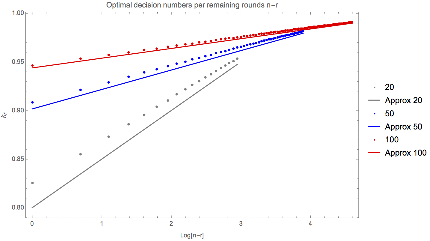
With increasing n, the decision numbers for the late rounds continue to increase, as the maximum of the remaining draws keeps increasing (Figure 15):

Figure 15: Decision numbers per round, n=100, GM and optimal

In fact, for large enough n there is a linear relationship between $k_{r}$ and $\log(n-r)$, as Figure 16 shows.

Figure 16: Optimal decision numbers per remaining rounds n-r, for different values of n

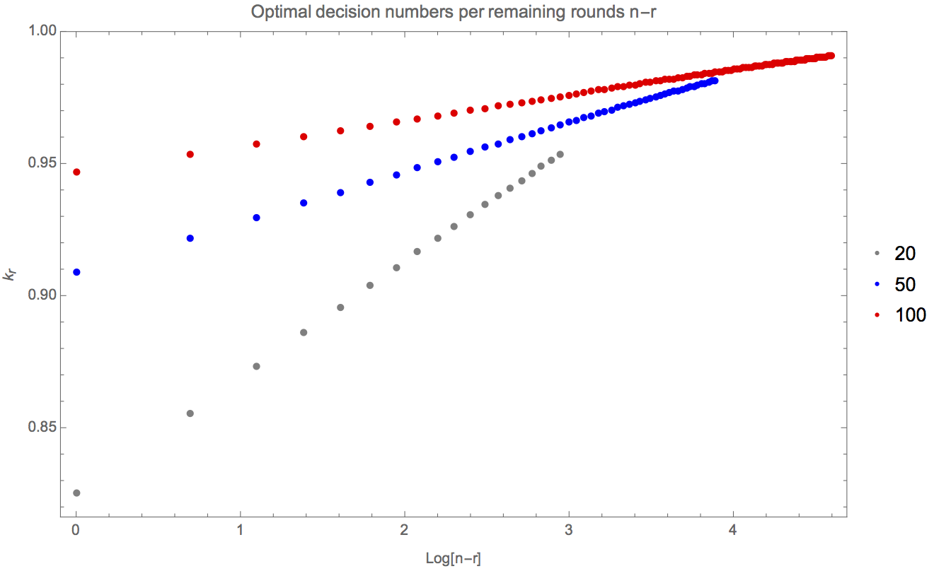
An intuitive approximation is:

$$k_{app1}(n,r)=\left(1-\frac{1}{n}\right)+\left(\frac{1}{n}\right)\cdot\log\left(\frac{n-r}{n}\right)$$ (23)

Which provides values slightly lower than those found by optimization (Figure 17). The first term comes from the naive strategy, and the 1/n multiplying the logarithm comes from observing how the slopes decrease with increasing n. The 1-1/n choice on the first round also has the property that the probability of a false positive is equal to the probability of a false negative in the first round. It is interesting that this qualitative approximation performs so well with a simple formula and without any arbitrary constants. A better approximation would have an intercept higher than $\left(1-\frac{1}{n}-\frac{\log n}{n}\right)$ and a slope lower than $\left(\frac{1}{n}\right)$, but not by much (the approximation gets better with increasing n).

Figure 17: Approximation for the optimal decision numbers per remaining rounds n-r, for different values of n

7 Simulation

The universe of the simulation is built generating 1000000 runs of 100 draws, and sampling the first n draws of each run. The evaluation function takes as arguments the array of decision numbers k and the array of draws a, returning a list {{v, fp, pg, mp}, m}, where v is 1 if the player won the game and 0 otherwise, fp is 1 if the game was lost due to a false positive and 0 otherwise, pg is the round in which the player accepted the draw, mp is the position of the maximum of a within a and m is the maximum of a. Given that information for each run of draws, one can process all the necessary statistics per round and overall quite quickly (3 different sets of decision numbers with n=10 were processed in less than 90 seconds).

The first test uses n=3, n=5 and n=10, and three strategies: naive, Gilbert and Mosteller and the new optimal strategy.

After testing that the position of the maximum is evenly distributed and that the expected value of the maximum is n/(n+1), the results are tallied per round (pg) and per result, with W determined by v=1, FP by v=0 and fp=1 and FN by v=0 and fp=0. These frequencies are then compared with the equations 16, 11 and 9. In the tallying table, each row corresponds to the same round (same pg); in the last round there’s only one value, corresponding to {1,0,n}. The error in the distribution of the maximum across the rounds is around 0.2%, so we present the results with 4 digits only.

naive	W				FP				FN
r	Realized		Predicted		Realized		Predicted		Realized		Predicted
1	0.	2349	0.	2346	0.	0987	0.	0988	0.	0991	0.	0988
2	0.	2423	0.	2423	0.	0826	0.	0826	0.	0418	0.	0417
3	0.	2010	0.	2014
Total	0.	6781	0.	6782

GM	W				FP				FN
r	Realized		Predicted		Realized		Predicted		Realized		Predicted
1	0.	2242	0.	2239	0.	0858	0.	0862	0.	1097	0.	1095
2	0.	2487	0.	2486	0.	0849	0.	0851	0.	0418	0.	0417
3	0.	2049	0.	2051
Total	0.	6777	0.	6776

Optimal	W				FP				FN
r	Realized		Predicted		Realized		Predicted		Realized		Predicted
1	0.	2314	0.	2319	0.	0955	0.	0954	0.	1015	0.	1014
2	0.	2318	0.	2315	0.	0689	0.	0691	0.	04543	0.	0541
3	0.	2166	0.	2165
Total	0.	6798	0.	6798

Table 15: Simulation results for n=3

naive	W				FP				FN
r	Realized		Predicted		Realized		Predicted		Realized		Predicted
1	0.	1347	0.	1345	0.	0654	0.	0655	0.	0653	0.	0655
2	0.	1362	0.	1362	0.	0634	0.	0632	0.	0472	0.	0475
3	0.	1357	0.	1362	0.	0584	0.	0587	0.	0264	0.	0263
4	0.	1275	0.	1269	0.	0464	0.	0464	0.	0063	0.	0063
5	0.	0871	0.	0868
Total	0.	6212	0.	6205

GM	W				FP				FN
r	Realized		Predicted		Realized		Predicted		Realized		Predicted
1	0.	1241	0.	1238	0.	0516	0.	0517	0.	0759	0.	0762
2	0.	1307	0.	1309	0.	0534	0.	0533	0.	0561	0.	0562
3	0.	1376	0.	1380	0.	0543	0.	0546	0.	0313	0.	0313
4	0.	1363	0.	1358	0.	0502	0.	0502	0.	0063	0.	0063
5	0.	0922	0.	0918
Total	0.	6209	0.	6203

Optimal	W				FP				FN
r	Realized		Predicted		Realized		Predicted		Realized		Predicted
1	0.	1316	0.	1313	0.	0610	0.	0611	0.	0684	0.	0687
2	0.	1313	0.	1314	0.	0558	0.	0558	0.	0532	0.	0533
3	0.	1289	0.	1294	0.	0458	0.	0462	0.	0368	0.	0367
4	0.	1249	0.	1243	0.	0305	0.	0305	0.	0187	0.	0188
5	0.	1130	0.	1125
Total	0.	6297	0.	6289

Table 16: Simulation results for n=5

naive	W				FP				FN
r	Realized		Predicted		Realized		Predicted		Realized		Predicted
1	0.	0650	0.	0651	0.	0351	0.	0349	0.	0349	0.	0349
2	0.	0653	0.	0653	0.	0346	0.	0346	0.	0306	0.	0307
…
9	0.	0431	0.	0431	0.	00179	0.	0180	0.	0001	0.	0001
10	0.	0254	0.	0253
Total	0.	5742	0.	5743

GM	W				FP				FN
r	Realized		Predicted		Realized		Predicted		Realized		Predicted
1	0.	0583	0.	0584	0.	0257	0.	0256	0.	0416	0.	0416
2	0.	0598	0.	0598	0.	0263	0.	0261	0.	0373	0.	0374
…
9	0.	0497	0.	0498	0.	0208	0.	0210	0.	0001	0.	0001
10	0.	0292	0.	0289
Total	0.	5770	0.	5772

Optimal	W				FP				FN
r	Realized		Predicted		Realized		Predicted		Realized		Predicted
1	0.	0628	0.	0629	0.	0318	0.	0315	0.	0370	0.	0371
2	0.	0629	0.	0630	0.	0308	0.	0307	0.	0334	0.	0335
…
9	0.	0542	0.	0542	0.	0095	0.	0095	0.	0045	0.	0045
10	0.	0492	0.	0492
Total	0.	5938	0.	5939

Table 17: Simulation results for n=10

The predictions match the simulations, and both show how for small n the naive strategy is close enough to the Gilbert and Mosteller results.

To confirm another important results, the simulations allow the comparison between the unconditional maximum of the n-1 draws (excluding the first round), which are equal to (n-1)/n, and the maximum of the n-1 draws left after the game goes to the second round (the C case, meaning no W, FP or FN in the first round), which is higher than (n-1)/n: {0.724, 0.824, 0.907} for n={3,5,10}.

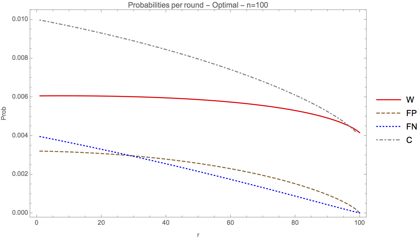
For n=100, the complete predictions by round and outcome were run, together with the 1000000 draws simulation. The charts reflect the predictions, since the simulation results continue to agree with the predictions.

Four sets of decision numbers were used: Naive, Girbert and Mollester, Optimal and Approximate (there was no need to use it below n=100, as the calculations can still be performed in a reasonable time and stored). The predicted overall win probabilities and the win frequency from the simulations can be found in Table 18.

n=100	Naive		GM		Optimal		Approximated
Predicted	0.	5304	0.	5405	0.	5651	0.	5632
Realized	0.	5306	0.	5411	0.	5650	0.	5634

Table 18: Win probabilities for different strategies, n=100

With n=100 the qualitative behavior of each strategy is clear, as the following charts (Figures ) of the probabilities per round for each strategy show. The probabilities for C are divided by the number of remaining rounds.

Figure 18: Probabilities per round - Naive and GM - n=100

Figure 19: Probabilities per round - Optimal and Approximated - n=100

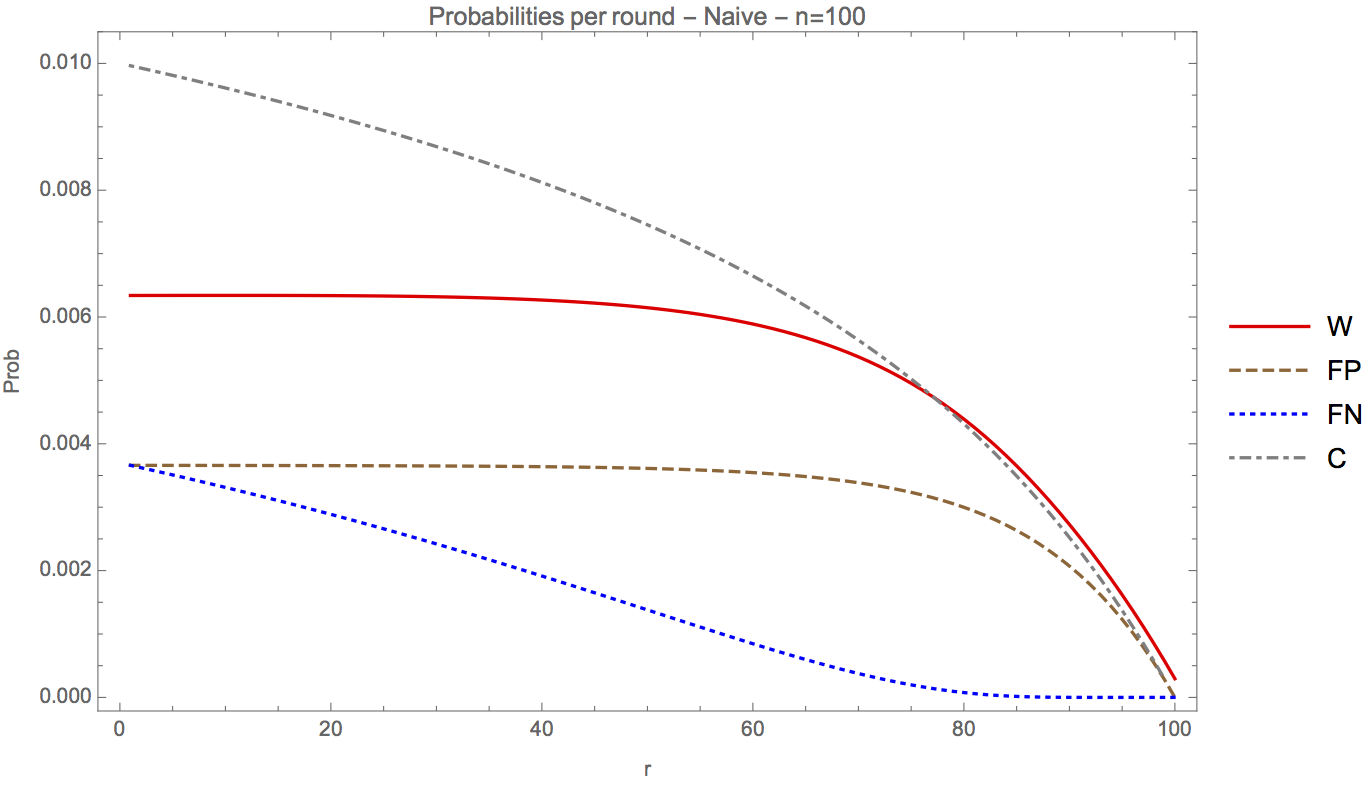
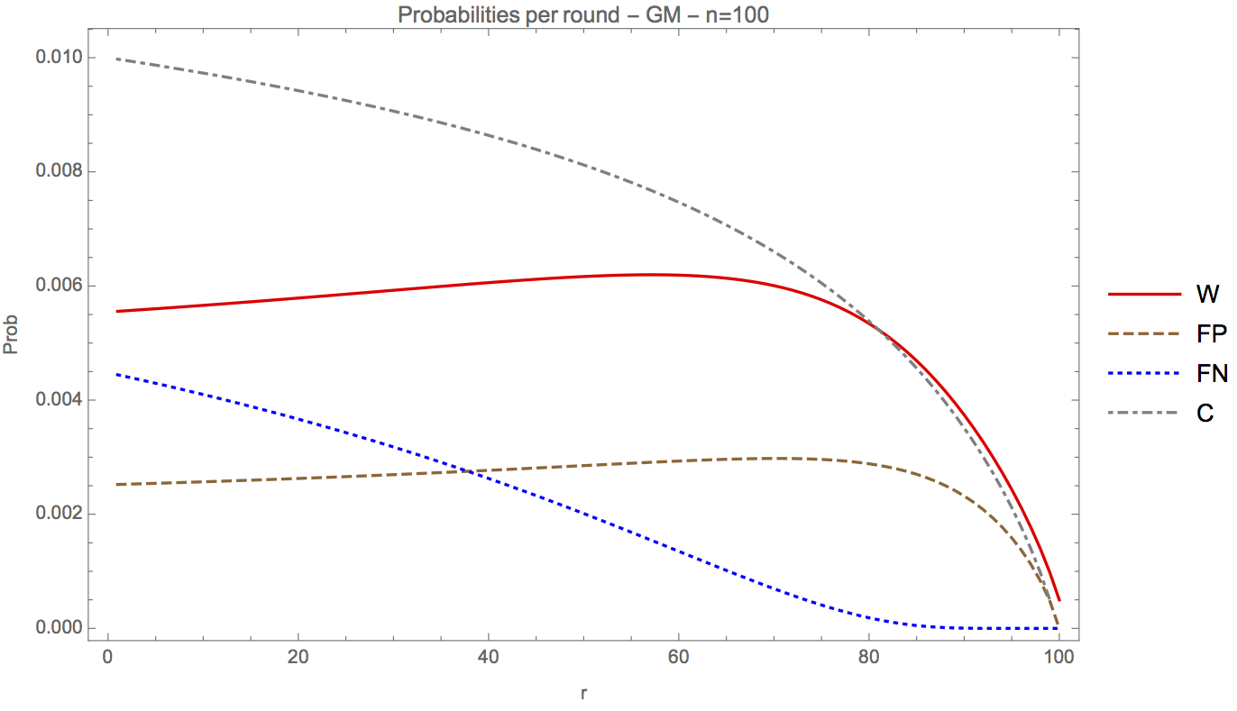
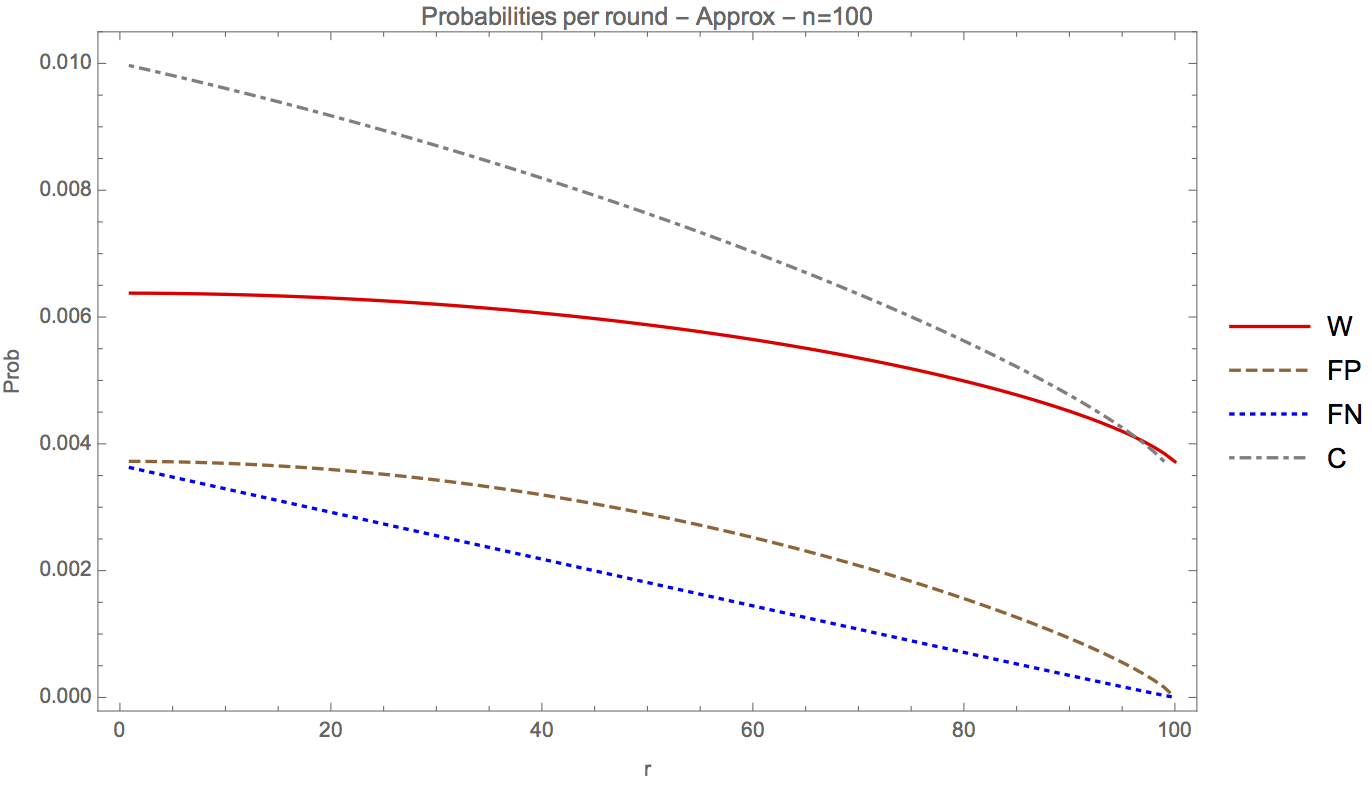
Both the Naive and the GM strategy have a persistent False Positive rate, flat or slowly increasing for more than half of the rounds, and the Win probability falls quickly just before the FP probability starts falling. On both cases the False Negative Rate decays linearly but with an early “target”, going to zero before the end of the draws.

In contrast, both the Optimal and the Approximated strategies have a slowly decreasing Win probability, a False Positive rate that starts it decrease at the start and a linearly decreasing False Negative rate with a “target” of n.

The price that the Naive and the GM strategies pay for lowering the decision numbers can be seen in the rapid decay of the probability of continuation of the game (normalized per remaining rounds).

Figure 20: Cumulative win probabilities per round - n=100

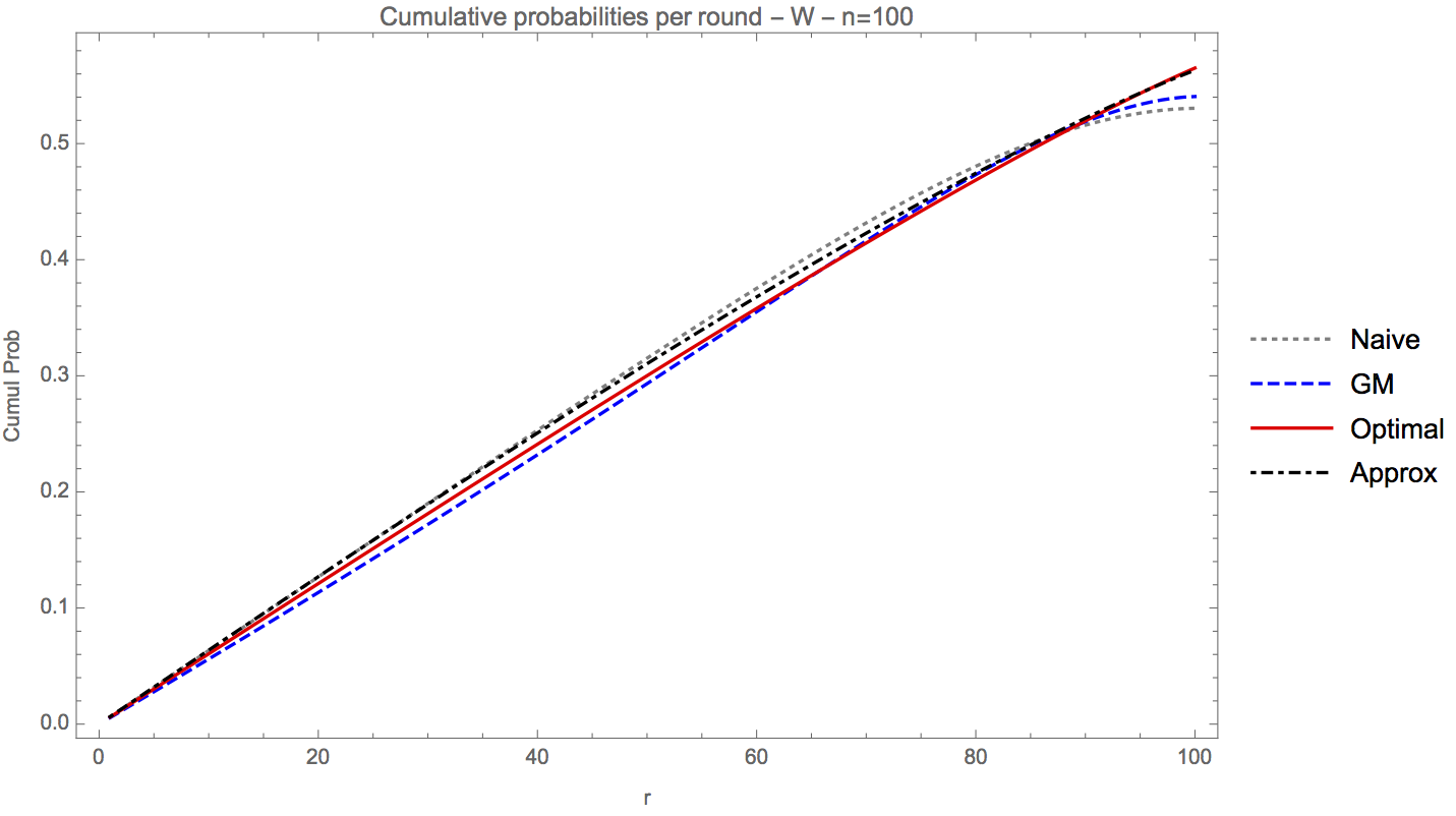
Figure 20 shows that the Naive strategy outperforms the others from round 24 to round 86, but at the end the Approximated strategy takes the lead, with the Optimal winning the overall contest on the last 5 rounds.

For larger n the value of the Naive and Approximated strategies increases, due to the ease of generating the decision numbers, and the time to process the probability of winning is about 3 minutes for n=1000. In contrast, it takes 1 minute to evaluate a simulation of 100000 runs and 1000 draws.

	Naive				Approximated
n	Predicted		Realized		Predicted		Realized
100	0.	5304	0.	5306	0.	5632	0.	5634
200	0.	5280			0.	5619
300	0.	5271			0.	5614
400	0.	5267			0.	5612
500	0.	5265			0.	5611
1000	0.	5260	0.	5247	0.	5608	0.	5585
2000	0.	5257	0.	5239	0.	5607	0.	5595

Table 19: Win probabilities for large n

The convergence implies a value close to 0.525 for the Naive strategy and 0.56 for the Approximated (and the Optimal) strategy, compared with 0.517 for the identical decision numbers case.

8 Conclusion

A new approach is developed for the full information game where n measurements from an uniform distribution are drawn and a player (knowing n) must decide at each draw whether or not to choose that draw with the goal to maximize the probability of choosing the draw that corresponds to the maximum of the sample. The approach includes an explicit equation for the probability of choosing the maximum at any round (the sum of this formula for all the rounds can be maximized to find the optimal decision numbers) and an approximation for large n that is easier to compute and produces a result very close to the optimal probability.

With this approach the error in the original Gilbert and Mosteller paper is attributed to the false negatives, which should be taken out of the universe of possibilities for the next rounds, therefore increasing the expected maximum at each round when compared with the unconditional expected value for n-r draws.

Another benefit of this approach is to make explicit the formulas for the probabilities of the four possible situations after each decision, enabling extensions of this problem where the payoff is different (including costs for each type of loss, costs for the continuation of the game or a round-dependent payoff).

This problem was posted on Cut the Knot by Alexander Bogomolny, and all the intuitions came after building (earlier and more inefficient) simulations. Once the visualizations for n=2 and n=3 were clear, with Mathematica handling the integration all that was left was to generalize the exponents f and coefficients g.

The author would like to thank Alexander Bogomolny for posting the problem and for creating an environment where people are supposed to try, fail and try again while enjoying the process.

References

- [1] ”Recognizing the Maximum of a Sequence”, John P. Gilbert and Frederick Mosteller, Journal of the American Statistical Association (1966), 61, pp. 35-73