Kinetic Properties of An Interplanetary Shock Propagating Inside a Coronal Mass Ejection

Abstract

We investigate the kinetic properties of a typical fast-mode shock inside an interplanetary coronal mass ejection (ICME) observed on 1998 August 6 at 1 AU, including particle distributions and wave analysis with the in situ measurements from Wind. Key results are obtained concerning the shock and the shock-ICME interaction at kinetic scales: (1) gyrating ions, which may provide energy dissipation at the shock in addition to wave-particle interactions, are observed around the shock ramp; (2) despite the enhanced proton temperature anisotropy of the shocked plasma, the low plasma $\beta$ inside the ICME constrains the shocked plasma under the thresholds of the ion cyclotron and mirror-mode instabilities; (3) whistler heat flux instabilities, which can pitch–angle scatter halo electrons through a cyclotron resonance, are observed around the shock, and can explain the disappearance of bidirectional electrons inside the ICME together with normal betatron acceleration; (4) whistler waves near the shock are likely associated with the whistler heat flux instabilities excited at the shock ramp, which is consistent with the result that the waves may originate from the shock ramp; (5) the whistlers share a similar characteristic with the shocklet whistlers observed by Wilson et al, providing possible evidence that the shock is decaying because of the strong magnetic field inside the ICME.

1 Introduction

Interplanetary (IP) shocks are driven by coronal mass ejections (CMEs) or fast solar wind. Interactions between CMEs often result in an interesting phenomenon: a shock overtakes and penetrates a preceding CME. CME–CME interactions are a frequent phenomenon near solar maximum because multiple CMEs can occur within one day (Liu et al., 2013). Shock–CME interactions are thus also frequent. Shock–CME interactions are of significance for both space weather predictions and basic plasma physics (e.g., Liu et al., 2012, 2014a, 2014b; Möstl et al., 2012; Lugaz et al., 2015). The studies of shock–CME interactions at kinetic scales, however, are very few.

Studies of shock kinetic properties mostly focus on the Earth’s bow shock (e.g., Wilson et al., 2014a, b; Möbius et al., 2001; Lee et al., 2009; Parks et al., 2012, 2013, 2017; Yang et al., 2014, 2016). There are some kinetic studies of IP shocks in the ambient solar wind (e.g., Richardson, 2010; Wilson et al., 2007, 2009, 2012; Blanco-Cano et al., 2016), but none inside interplanetary CMEs (ICMEs). A well-known and long investigated feature of the Earth’s bow shock is the waves and reflected particles dominant in the foreshock region. The statistics of Lugaz et al. (2015) suggest that most of the shocks inside ICMEs (low-$\beta$ plasma) are relatively weak, while Sckopke et al. (1983) find that leading or trailing wave trains are usually generated around low-Mach number low-$\beta$ shocks. Previous investigations of the waves associated with IP shocks in the ambient solar wind indicate that whistler waves play an important role in shock dynamics (e.g., Wilson et al., 2009, 2012, 2017; Kajdič et al., 2012; Ramírez Vélez et al., 2012). Theory and observations suggest that low Mach number shocks mainly rely upon wave dispersion for energy dissipation (Kennel et al., 1985; Wilson et al., 2017). Gyrating ions, some of the particles reflected by the shock and gyrating around the local magnetic field, are thought to provide possible free energy for the waves near a supercritical shock (Wilson et al., 2012).

Owing to the strong magnetic field and low plasma $\beta$ of ICMEs, a shock inside an ICME is expected to have interesting properties at kinetic scales. Investigations of shock-ICME interactions so far have mainly focused on the large scale, but not on the kinetic scale processes, such as the particle kinetic behaviors and waves. Suprathermal electrons flowing in both directions along the magnetic field, called bi-directional electrons (BDEs), have been identified as a good indicator of an ICME (e.g., Gosling et al., 1987). A question thus arises regarding how a shock inside an ICME influences BDEs. Examining the particle populations and waves around a shock inside an ICME may provide a new perspective about shock–ICME interactions.

In this Letter, we analyze an IP shock inside an ICME with the in situ measurements from Wind/MFI (Lepping et al., 1995) and Wind/3DP (Lin et al., 1995) at kinetic scales. The shock was propagating in an ICME at 1AU around 07:16:07 UT on 1998 August 6. Burst–mode particle data (full distribution every 3 seconds) from Wind/3DP around the shock are available except that the EESA-High particle detector only has the survey–mode data. With the high–cadence magnetic field data (11 samples/s) and the burst–mode particle data, we carry out a first kinetic investigation of the shock-inside-ICME phenomenon using the chosen case, including particle distributions (in Section 2.1) and wave analysis (in Section 2.2). The results provide new insights on the kinetic physical processes involved in shock-ICME interactions.

2 Observations and Results

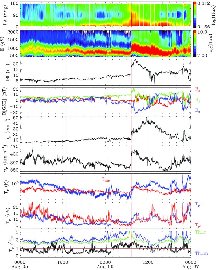
Figure 1: Solar wind measurements around the 1998 August 06 shock event from Wind. From top to bottom, the panels show the pitch angle distribution of 340 eV electrons, ion energy spectrum, magnetic field strength and GSE components, proton density, bulk speed, proton temperature (expected proton temperature in red), proton temperature perpendicular (blue) and parallel (red) to magnetic field, the ratio of the perpendicular temperature to the parallel temperature, and thresholds of ion cyclotron (green) and mirror-mode (blue) instabilities. The region between the two blue vertical lines is the ICME interval, and the red vertical line marks the shock propagating in the ICME.

Figure 1 shows an overview of the solar wind parameters around the IP shock observed on 1998 August 6 at Wind. The whole time interval of the ICME is about 23 hours. The shock has propagated deep into the ICME. The ICME shown in Figure 1 was first identified by Richardson & Cane (2010), and then analyzed together with the shock by Lugaz et al. (2015) at large scales. The ICME is characterized by a lower-than-expected proton temperature, enhanced magnetic field strength and relatively smooth rotation of the magnetic field vector. BDEs, a typical signature of ICMEs, are observed as shown in the top panel of Figure 1. The disappearance of BDEs after the shock may be explained partly by the pitch-angle scattering by the whistler heat flux instabilities observed near the shock ramp (see Section 2.2). The basic parameters of the shock are obtained from the shock database maintained by J. C. Kasper (https://www.cfa.harvard.edu/shocks/). The shock is a low-Mach number (${M}_{f}$ $\sim$1.59) low-$\beta$ ($\sim$ 0.07) case. It is a fast-mode quasi-perpendicular shock, with a shock normal angle ${\theta}_{Bn}$ = ${80}{\arcdeg}$ $\pm$ ${5}{\arcdeg}$ and a shock speed ${V}_{shn}$ = ${478.8}$ $\pm$ ${36.5}$ km s^-1.

2.1 Particle Velocity Distributions

Figure 2 (top) gives the ion distributions obtained from the 3DP/PESA-High instrument around the shock ramp. The IP shock shows evidence for perpendicular ion heating, i.e., the main red beam structure is broadened much further in the direction perpendicular to the local magnetic field across the shock than in the parallel direction. A preferential perpendicular heating by the shock is also illustrated in Figure 1 by the enhanced T_p⊥/T_p∥ across the shock. This result is consistent with the picture of a quasi-perpendicular shock (e.g., Liu et al., 2007). Liu et al. (2006, 2007) suggest that mirror-mode instabilities resulting from high proton temperature anisotropy and high plasma $\beta$ may be excited in the downstream of a quasi-perpendicular shock. In our case, the proton temperature anisotropy of the shocked plasma is high, but the plasma $\beta$ ($\sim$0.07) is low since this is within an ICME. The low plasma $\beta$ inside the ICME inhibits mirror–mode and ion cyclotron instabilities.

We find beam-like populations of gyrating ions (indicated by black arrows) in Figure 2b, with the velocity being about 240 km s^-1. The velocity is consistent with the estimate from a specular reflection theory (Gosling et al., 1982). The beam at the positive region of $V_{perp}$ is relatively weak. Similarly, Figure 2c gives evidence (indicated by black arrows) for gyrating ions in the downstream of the shock with a relatively smaller density than those in Figure 2b. Our results on the gyrating ions are in agreement of the bow shock observations (Sckopke et al., 1983) and the specular reflection theory (Gosling et al., 1982).

Gyrating ions are usually observed in association with the magnetic foot and overshoot of quasi-perpendicular supercritical shocks due to specular reflection (e.g., Paschmann et al., 1980, 1982; Sckopke et al., 1983; Thomsen et al., 1985). Foot thickness roughly represents the longest distance that the specularly-reflected ions can propagate to the upstream of the shock (Livesey et al., 1984; Gosling & Thomsen, 1985). The predicted foot thickness based on the expression from Livesey et al. (1984) is $d\sim$ 72.7 km, and the corresponding time length is $d/{V}_{p}\sim$ 0.196 s. Magnetic field observations of this shock display a transition without an obvious foot structure (see Section 2.2). The time resolution of the magnetic field data is about 11 samples/s, so very few magnetic samples are obtained within the predicted time length of the foot structure. Therefore, we consider that the lack of an obvious foot structure of the shock may be due to undersampling and may not reflect the realistic magnetic transition of the shock.

Figure 2 (bottom) presents the evolution of the electron distributions from the 3DP/EESA-High instrument across the shock ramp. There are obvious beam features indicated by the black arrows in Figure 2d and Figure 2e along the directions parallel and anti-parallel to the magnetic field. The velocity of the field-aligned beam structures ranges from 5000 km s^-1 to 6000 km s^-1, and the corresponding energy range of the field-aligned beam is approximately 278 eV-400 eV. The energy of BDEs shown in Figure 1 is 340 eV. Therefore, the field-aligned beams correspond to the BDEs observed inside the ICME. In the downstream of the shock as shown in Figure 2f, the field-aligned beams disappear. These results are consistent with what is shown in Figure 1 (top panel).

2.2 Wave Analysis

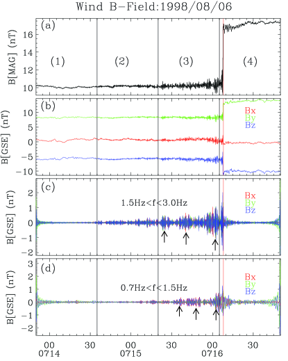
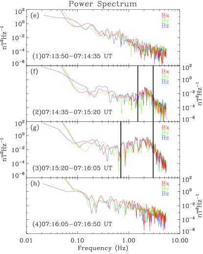
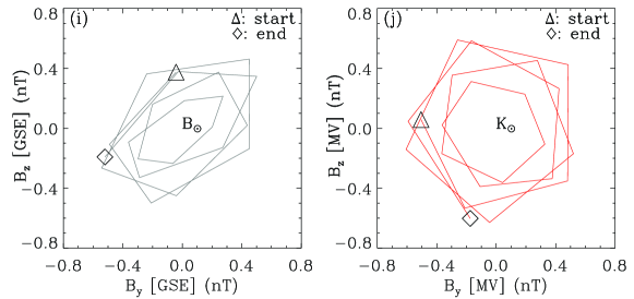
Figure 3: Magnetic field measurements and variance analysis. (a-d) Magnetic field fluctuations across the shock. From top to bottom, the panels show the magnitude of the magnetic field, the GSE components of the magnetic field, the filtered GSE components at 1.5 Hz $<$ f $<$ 3.0 Hz, and the filtered GSE components at 0.7 Hz $<$ f $<$ 1.5 Hz, respectively. The red vertical line denotes the shock arrival, and the three black vertical lines give four 45-second time intervals marked as (1), (2), (3) and (4) corresponding to the four intervals of the right panels. (e-h) Power spectra derived with a standard FFT technique. The regions between the two black vertical lines in panels (f) and (g) indicate the peak frequency ranges of the power spectra. (i-j) An example of MV analysis of the waves (1.5Hz <f <3.0Hz, $\lambda$₂/ $\lambda$₃=59.764, $\lambda$₁/$\lambda$₂=1.085, $\hat{K}_{GSE}$= $[$0.624, 0.487, -0.610$]$, $\theta_{kB}$= $39^{\circ}$ (or $141^{\circ}$), $\theta_{kn}$= $39.7^{\circ}$ (or $140.3^{\circ}$), $\theta_{kV}$= $53.7^{\circ}$ (or $126.3^{\circ}$)) between 07:15:23 UT

Figure 3 shows the Wind/MFI data at the cadence of 11 samples/s across the shock, the power spectra of the magnetic field components and a minimum variance (MV) analysis example. Across the shock, the magnetic field is enhanced. This field jump lasts for $\sim$2 s, much longer than the electron cyclotron period $T_{ce}$ (0.00198 s $<$ $T_{ce}$ $<$ 0.00357 s). Therefore, the first adiabatic invariant $\mu$=E_⊥/B should be conserved during the compression, which means that normal betatron acceleration of electrons may exist. Normal betatron acceleration of electrons mainly occurs before the shock, since the magnetic field almost remains the same in the downstream of the shock. The normal betatron acceleration of electrons may contribute to the change of the pitch angle of BDEs (Fu et al., 2012). Waves are observed around the shock, and the peak frequency of the waves is 0.7 Hz $<$ $f$ $<$ 3.0 Hz. The waves may be triggered at the shock ramp, since the amplitudes of these wave packets decrease from the shock ramp to the upstream. By comparing the first three obvious wave packets (indicated by black arrows) near the shock ramp at 1.5 $\sim$ 3.0 Hz with those at 0.7 $\sim$ 1.5 Hz, we find that the high frequency wave packets occur about 10 seconds ahead of the low frequency envelopes. This frequency dependence is consistent with that of whistler waves, whose group velocities increase with increasing frequency.

We perform a MV analysis (Khrabrov & Sonnerup, 1998) of the magnetic fluctuations to determine the wave vector ($\hat{K}_{GSE}$), polarizations with respect to the ambient magnetic field and $\hat{K}_{GSE}$, and wave vector angles with respect to the local magnetic field $(\theta_{kB})$, shock normal vector $(\theta_{kn})$ and local solar wind velocity $(\theta_{kV})$. Since the upstream magnetic field and solar wind velocity are roughly constant, we use the average values obtained from the cfa shock database: $\hat{B}$=(-0.4, 8.3, -6.1) nT and $\hat{V}_{sw}$=(-371.8, -21.1, -2.9) km s^-1. Bandpass filters are applied to the waveforms prior to the MV analysis on specific subintervals following the procedure of Wilson et al. (2009), which requires the ratio of the intermediate to minimum eigenvalues $\lambda$₂/$\lambda$₃ $>$10 to get a reasonable result. We choose 18 specific subintervals from 07:14:35 UT to 07:16:05 UT for the MV analysis with the frequency range: $f_{cp}$ $<$ 0.7 Hz $<$ $f$ $<$ 3.0 Hz $<$ $f_{ce}$, where $f_{cp}$ and $f_{ce}$ represent the proton gyro-frequency and electron gyro-frequency, respectively. Figure 3i and Figure 3j display hodograms of the magnetic field in GSE and MV coordinates. Since the X component of the magnetic field is almost zero (refer to Figure 3b), only the hodogram with $B_{z}$ versus $B_{y}$ shows the meaningful polarization with respect to the magnetic field. The wave event is right-hand (RH) polarized (Figure 3i) with respect to the magnetic field in the spacecraft frame. Also, the wave event is nearly circularly RH polarized with respect to $\hat{K}_{GSE}$.

In total, the wave polarizations for the 18 subintervals with respect to $\hat{K}_{GSE}$ are: 7 samples exhibit LH sense and 11 samples present RH sense. The different polarizations of the wave events with respect to $\hat{K}_{GSE}$ can be explained by the ambiguity of the sign of $\hat{K}_{GSE}$ due to projection effects, which result from single satellite magnetic field measurements (Khrabrov & Sonnerup, 1998). All the waveforms show RH polarization with respect to the local magnetic field just like the example shown in Figure 3i, which is a characteristic of whistler waves. Since the MV analysis is performed in the spacecraft frame, we first handle the Doppler effects following the method outlined in Wilson et al. (2017) and then calculate the phase velocity of the whistler waves $(V_{ph})$, based on a cold plasma assumption. We obtain that $V_{ph}$ is about 206 km s^-1, which is larger than the local solar wind velocity along $\hat{K}_{GSE}$ (about 185 km s^-1). This suggests that the waves could be detected in their true sense of polarization with respect to the local magnetic field.

The values of $\theta_{kB}$, $\theta_{kn}$ and $\theta_{kV}$ of the waves examined here exhibit broad ranges, consistent with the theory of (Wu et al., 1983) and prior observations (e.g., Wilson et al., 2009, 2012, 2017; Sundkvist et al., 2012). The specific ranges of the angles are : $5.6^{\circ}$$<$ $\theta_{kB}$ $<$ $71.8^{\circ}$, $31.7^{\circ}$ $<$ $\theta_{kn}$ $<$ $74.0^{\circ}$ and $31.1^{\circ}$ $<$ $\theta_{kV}$ $<$ $81.5^{\circ}$. Compared with the observations of Wilson et al. (2009, 2017), the whistler waves in this case are similar to the shocklet whistlers. Both of them have a broad range of $\theta_{kB}$ and tend to be more oblique than the precursor whistler waves. Most of the wave samples in this Letter have $31.7^{\circ}$ $<$ $\theta_{kn}$ $<$ $74.0^{\circ}$, so they are not likely phase standing (Mellott & Greenstadt, 1984).

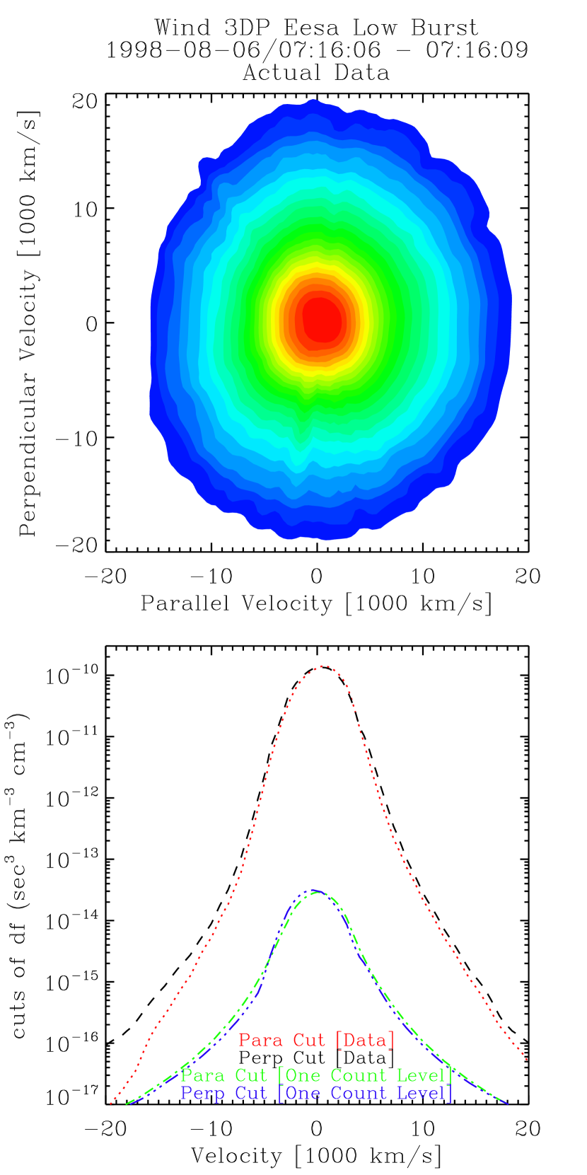
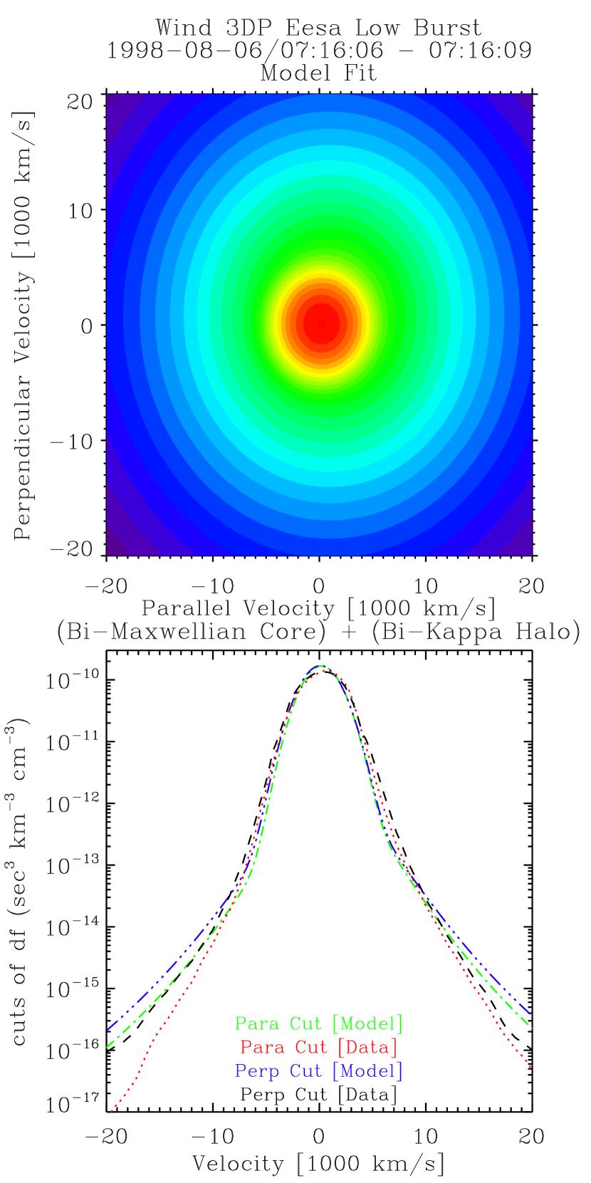
Figure 4: An example showing the comparison between the observed (left) and fitted (right) electron distributions from the 3DP/EESA-Low instrument. The top row shows the contours of the distributions. The X and Y axis denote the velocities parallel and perpendicular to the ambient magnetic field, respectively. The bottom row presents the parallel and perpendicular cuts of the distributions and corresponding one-count level cuts. The one-count level cuts are lower than the observed value at each velocity, indicating that the measurements are reliable.

A relationship between whistler mode generation and electrons has been presented by previous studies (e.g., Gary et al., 1994, 1999; Wilson et al., 2009). Gary et al. (1999) demonstrate that the heat flux driven whistler mode is always unstable when the temperature anisotropy of halo electrons T_⊥h/T_∥h $>$ 1.01 and always stable when the parallel beta of core electrons $\beta$_∥c $\leqslant$ 0.25. The primary influence on halo electrons of whistler heat flux instabilities is to pitch angle scatter them through a cyclotron resonance. Table 1 shows statistics about the electron parameters derived from the 3DP/EESA-Low data. We fit core electrons to Bi-Maxwellian distributions and halo electrons to Bi-Kappa distributions (Mace & Sydora, 2010). Figure 4 presents the observed and fitted electron distributions. The difference between the logarithms of the average observed and model distribution functions is less than 0.1, so the fittings are relatively good. The uncertainties of the parameters, such as the parallel/perpendicular temperatures and the number density of core/halo electrons, are in general less than 5% of the corresponding values. From 07:16:06 UT to 07:16:09 UT, whistler heat flux instabilities arise, which is a possible driver of the whistler waves. The shock ramp is located at about 07:16:07 UT, which is near the time of the whistler heat flux instabilities, so the waves are likely produced at the shock ramp. In Table 1, a clear increase in T_⊥h/T_∥h is seen across the shock (07:16:03–07:16:09 UT), which may result from the normal cyclotron resonance that can increase the transverse energy of the electrons and normal betatron acceleration of electrons. In the downstream of the shock (07:16:07–07:16:12 UT), although normal betatron acceleration almost does not contribute to the acceleration any more, T_⊥h/T_∥h still increases but at a slower rate. These results illustrate that whistler heat flux instabilities may account for the disappearance of the BDEs inside the ICME through pitch-angle scattering together with normal betatron acceleration. T_⊥c/T_∥c follows the same pattern, but the increase is not so dramatic. In addition, T_⊥h/T_∥h increases at a faster rate across the shock than T_∥h/T_∥c decreases, in agreement with the observation results by Wilson et al. (2009) and simulation results by Gary et al. (1994). Note that there are deviations between the fit curves and the data at $V>10^{4}$ km s^-1. The relative deviation for the parallel cut is larger than that for the perpendicular cut, so the actual T_⊥h/T_∥h should be larger than those in Table 1. This implies that the electron distributions would be more unstable.

3 Summary and Discussions

This Letter presents the first analysis of kinetic properties of an IP shock propagating inside an ICME on 1998 August 6, combining the particle (both ion and electron) distributions and wave analysis. Key findings are obtained concerning how shock-ICME interaction behaves at kinetic scales:

1. Gyrating ions are observed around the shock, which is consistent with theoretical predictions and bow shock observations, and give evidence that particle reflection may occur even at low Mach number shocks. Reflected ions observed in this case may provide a venue for energy dissipation around the shock together with the waves observed near the shock. The shock lacks an obvious foot structure; however, the existence of gyrating ions implies that the foot structure may be under-sampled. In addition, although the shock produces enhanced proton temperature anisotropy in the downstream of the shock, the shocked ICME plasma is under the thresholds of the ion cyclotron and mirror-mode instabilities because of the low plasma $\beta$ inside the ICME.

2. The disappearance of BDEs downstream of the shock characterizes the interaction between the shock and ICME. This is probably caused by the pitch-angle scattering of the electrons by the waves observed near the shock ramp. The electron distribution around the shock meets the criteria to excite whistler heat flux instabilities, which may contribute to the wave generation and help explain the disappearance of the BDEs downstream of the shock. Another mechanism that may also help explain the disappearance of the BDEs inside the ICME is the normal betatron acceleration that occurs across the shock.

3. The waves around the shock are thought to be whistler waves, as the higher-frequency wave envelopes occur earlier and all the wave events show RH polarization with respect to the ambient magnetic field. The whistler waves are probably associated with the electron distribution unstable to whistler heat flux instabilities observed around the shock. The waves may originate from the shock ramp, since the amplitudes of the wave packets decrease from the shock ramp to the upstream. This is consistent with the result that the whistler heat flux instabilities are excited at the shock ramp. The whistler waves share a similar characteristic with the shocklet (steepened magnetosonic waves) whistlers, which likely suggests that the shock may be decaying due to the shock-ICME interaction. The shock has propagated deep into the ICME, so the shock may have begun to decay because of the strong magnetic field inside the ICME.

Figure 2: The evolution of the ion (top) and electron (bottom) distributions (in the solar wind frame) across the shock ramp. The contours show constant phase space density in the plane containing the ambient magnetic field (horizontal axis) and local solar wind velocity. Projected onto the planes are the following: shock normal direction (dashed red line), shock surface (solid red line), and solar wind velocity direction (solid black line).

and 07:15:25 UT. The hodograms in GSE (i) and MV (j) coordinates are shown. The [X,Y,Z]-MV coordinates represent the directions parallel to the minimum, intermediate and maximum variance eigenvectors, respectively.

Table 1: Wind 3DP electron parameters from Eesa Low Burst Mode Data

Time(UT)	T⊥c/T∥c	T⊥h/T∥h	T∥h/T∥c	$\beta$∥c	nce(cm-3)	nhe(cm-3)	nhe/nce
07:16:00–07:16:03	0.93	0.76	18.01	0.467	8.66	0.383	0.044
07:16:03–07:16:06	0.94	0.77	18.04	0.469	8.76	0.387	0.044
07:16:06–07:16:09	1.08	1.17	12.69	0.310	10.47	0.656	0.063
07:16:09–07:16:12	1.15	1.47	10.81	0.202	11.16	0.786	0.070
07:16:12–07:16:16	1.16	1.48	10.80	0.213	11.12	0.799	0.072

References

- Blanco-Cano et al. (2016) Blanco-Cano, X., Kajdič, P., Aguilar-Rodríguez, E., et al. 2016, J. Geophys. Res., 121, 992
- Fu et al. (2012) Fu, H. S., Cao, J. B., Mozer, F. S., Lu, H. Y., & Yang, B. 2012, J. Geophys. Res., 117, A01203
- Gary et al. (1994) Gary, S. P., Scime, E. E., Phillips, J. L., & Feldman, W. C. 1994, J. Geophys. Res., 99, 23
- Gary et al. (1999) Gary, S. P., Skoug, R. M., & Daughton, W. 1999, Physics of Plasmas, 6, 2607
- Gosling et al. (1987) Gosling, J. T., Baker, D. N., Bame, S. J., et al. 1987, J. Geophys. Res., 92, 8519
- Gosling & Thomsen (1985) Gosling, J. T., & Thomsen, M. F. 1985, J. Geophys. Res., 90, 9893
- Gosling et al. (1982) Gosling, J. T., Thomsen, M. F., Bame, S. J., et al. 1982, Geophys. Res. Lett., 9, 1333
- Kajdič et al. (2012) Kajdič, P., Blanco-Cano, X., Aguilar-Rodriguez, E., et al. 2012, J. Geophys. Res., 117, A06103
- Kennel et al. (1985) Kennel, C. F., Edmiston, J. P., & Hada, T. 1985, Washington DC American Geophysical Union Geophysical Monograph Series, 34, 1
- Khrabrov & Sonnerup (1998) Khrabrov, A. V., & Sonnerup, B. U. Ö. 1998, J. Geophys. Res., 103, 6641
- Lee et al. (2009) Lee, E., Parks, G. K., Wilber, M., & Lin, N. 2009, Phys. Rev. Lett., 103, 031101
- Lepping et al. (1995) Lepping, R. P., Acũna, M. H., Burlaga, L. F., et al. 1995, Space Sci. Rev., 71, 207
- Lin et al. (1995) Lin, R. P., Anderson, K. A., Ashford, S., et al. 1995, Space Sci. Rev., 71, 125
- Liu et al. (2007) Liu, Y., Richardson, J. D., Belcher, J. W., & Kasper, J. C. 2007, ApJ, 659, L65
- Liu et al. (2006) Liu, Y., Richardson, J. D., Belcher, J. W., Kasper, J. C., & Skoug, R. M. 2006, J. Geophys. Res., 111, A09108
- Liu et al. (2013) Liu, Y. D., Luhmann, J. G., Lugaz, N., et al. 2013, ApJ, 769, 45
- Liu et al. (2014a) Liu, Y. D., Yang, Z., Wang, R., et al. 2014a, ApJ, 793, L41
- Liu et al. (2012) Liu, Y. D., Luhmann, J. G., Möstl, C., et al. 2012, ApJ, 746, L15
- Liu et al. (2014b) Liu, Y. D., Luhmann, J. G., Kajdič, P., et al. 2014b, Nat. Commun, 5, 3481
- Livesey et al. (1984) Livesey, W. A., Russell, C. T., & Kennel, C. F. 1984, J. Geophys. Res., 89, 6824
- Lugaz et al. (2015) Lugaz, N., Farrugia, C. J., Smith, C. W., & Paulson, K. 2015, J. Geophys. Res., 120, 2409
- Mace & Sydora (2010) Mace, R. L., & Sydora, R. D. 2010, J. Geophys. Res., 115, A07206
- Mellott & Greenstadt (1984) Mellott, M. M., & Greenstadt, E. W. 1984, J. Geophys. Res., 89, 2151
- Möbius et al. (2001) Möbius, E., Kucharek, H., Mouikis, C., et al. 2001, Annales Geophysicae, 19, 1411
- Möstl et al. (2012) Möstl, C., Farrugia, C. J., Kilpua, E. K. J., et al. 2012, ApJ, 758, 10
- Parks et al. (2017) Parks, G. K., Lee, E., Fu, S. Y., et al. 2017, Reviews of Modern Plasma Physics, 1, 1
- Parks et al. (2012) Parks, G. K., Lee, E., McCarthy, M., et al. 2012, Phys. Rev. Lett., 108, 061102
- Parks et al. (2013) Parks, G. K., Lee, E., Lin, N., et al. 2013, ApJ, 771, L39
- Paschmann et al. (1980) Paschmann, G., Sckopke, N., Asbridge, J. R., Bame, S. J., & Gosling, J. T. 1980, J. Geophys. Res., 85, 4689
- Paschmann et al. (1982) Paschmann, G., Sckopke, N., Bame, S. J., & Gosling, J. T. 1982, Geophys. Res. Lett., 9, 881
- Ramírez Vélez et al. (2012) Ramírez Vélez, J. C., Blanco-Cano, X., Aguilar-Rodriguez, E., et al. 2012, J. Geophys. Res., 117, A11103
- Richardson & Cane (2010) Richardson, I. G., & Cane, H. V. 2010, Sol. Phys., 264, 189
- Richardson (2010) Richardson, J. D. 2010, Geophys. Res. Lett., 37, L12105
- Sckopke et al. (1983) Sckopke, N., Paschmann, G., Bame, S. J., Gosling, J. T., & Russell, C. T. 1983, J. Geophys. Res., 88, 6121
- Sundkvist et al. (2012) Sundkvist, D., Krasnoselskikh, V., Bale, S. D., et al. 2012, Phys. Rev. Lett., 108, 025002
- Thomsen et al. (1985) Thomsen, M. F., Gosling, J. T., Bame, S. J., & Rusell, C. T. 1985, J. Geophys. Res., 90, 267
- Wilson et al. (2014a) Wilson, L. B., Sibeck, D. G., Breneman, A. W., et al. 2014a, J. Geophys. Res., 119, 6455
- Wilson et al. (2014b) —. 2014b, J. Geophys. Res., 119, 6475
- Wilson et al. (2007) Wilson, III, L. B., Cattell, C., Kellogg, P. J., et al. 2007, Phys. Rev. Lett., 99, 041101
- Wilson et al. (2009) Wilson, III, L. B., Cattell, C. A., Kellogg, P. J., et al. 2009, J. Geophys. Res., 114, A10106
- Wilson et al. (2017) Wilson, III, L. B., Koval, A., Szabo, A., et al. 2017, J. Geophys. Res., 122, 9115
- Wilson et al. (2012) —. 2012, Geophys. Res. Lett., 39, L08109
- Wu et al. (1983) Wu, C. S., Zhou, Y. M., Tsai, S., et al. 1983, The Physics of Fluids, 26, 1259
- Yang et al. (2016) Yang, Z., Huang, C., Liu, Y. D., et al. 2016, ApJS, 225, 13
- Yang et al. (2014) Yang, Z., Liu, Y. D., Parks, G. K., et al. 2014, ApJ, 793, L11