Wide-area tomography of CMB lensing and the growth of cosmological density fluctuations

Abstract

We describe a tomographic dissection of the Planck CMB lensing data, cross-correlating this map with galaxies in different ranges of photometric redshift. We use the nearly all-sky 2MPZ and WISE$\times$SCOS catalogues for $z<0.35$, extending to $z<0.6$ using SDSS. We describe checks for consistency between the different datasets, and perform a test for possible leakage of thermal Sunyaev–Zel’dovich signal into our cross-correlation measurements. The amplitude of the cross-correlation allows us to estimate the evolution of density fluctuations as a function of redshift, thus providing a test of theories of modified gravity. Assuming the common parametrisation for the logarithmic growth rate, $f_{g}=\Omega_{m}(z)^{\gamma}$, we infer $\gamma=0.77\pm 0.18$ when $\Omega_{m}$ is fixed using external data. Thus CMB lensing tomography is currently consistent with Einstein gravity, where $\gamma=0.55$ is expected. We discuss how such constraints may be expected to improve with future data.

1 Introduction

One of the more remarkable results of the Planck mission has been its measurement of the impact of foreground mass inhomogeneities on cosmic microwave background (CMB) fluctuations. Gravitational lensing by large-scale structure (LSS) distorts the background Gaussian CMB sky and imprints non-Gaussian signatures, whose detection allows the degree of gravitational lensing to be inferred; this in turn yields a map of the projection of density fluctuations times a distance-dependent kernel (see e.g Lewis & Challinor 2006). We then obtain an astonishing picture containing imprints of every void or supercluster that ever existed, projected against the backlight of the CMB.

CMB lensing was first detected by Smith et al. (2007) from cross-correlation of the Wilkinson Microwave Anisotropy Probe (WMAP) data with radio galaxy counts from the NRAO VLA Sky Survey (NVSS), and then confirmed by Hirata et al. (2008) where WMAP with a more extended set of LSS tracers was used. The first measurements of this effect directly from auto-correlation of CMB data were presented by Das et al. (2011) using the Atacama Cosmology Telescope (ACT) and by van Engelen et al. (2012) from the South Pole Telescope (SPT). Holder et al. (2013) also showed that the SPT lensing map correlated with the high-$z$ cosmic infrared background. These results were followed by all-sky CMB lensing analyses from the Planck satellite via reconstruction techniques. The initial implementation of this approach in Planck Collaboration (2014) was then improved by including polarization data, which raised the total $S/N$ of lensing detection to about 40 (Planck Collaboration 2016b).

The main effect derives from mass fluctuations at redshifts $z\simeq 2$, set by a balance between geometrical factors that favour distant lenses, and the fact that LSS grows with time. This measure of structure at intermediate redshifts is a valuable complement to the intrinsic CMB fluctuations at $z\gg 1$, and breaks degeneracies that exist between cosmological parameters inferred using CMB data alone (Sherwin et al., 2011). The Planck lensing measurements are closely consistent with a standard flat $\Lambda$CDM model with $\Omega_{m}\simeq 0.3$, and provide strong evidence for this model independent of alternative powerful probes (SNe; BAO); see Planck Collaboration (2016a), Betoule et al. (2014), Alam et al. (2017).

But although the CMB lensing kernel peaks at high redshift, the signal is broadly distributed and significant lensing contributions are made from LSS down to local redshifts, $z\sim 0.1$ (Lewis & Challinor 2006). This opens the possibility of using CMB lensing to measure the growth of structure with time, provided the contributions to CMB lensing from the different redshifts can be disentangled – which can be achieved via cross-correlation if we have a set of foreground galaxies of known redshift. In that case, one can carry out a tomographic analysis in which the galaxies are split into a number of broad redshift bins; for each of these the galaxy autocorrelation and cross-correlation with the CMB lensing signal can be measured. Both these correlations are proportional on large scales to the matter power spectrum at the redshift concerned, times either $b^{2}$ or $b$ for auto- and cross-correlation, where $b$ is the linear galaxy bias parameter. Thus both $b$ and the amplitude of matter fluctuations as a function of redshift can be inferred.

Such measurements of the growth of density fluctuations are of great interest. At the simplest level, the linear growth history is predicted once the cosmological parameters are set; thus growth measurements are useful additional information helping to pin down the parameters. But the real interest comes in looking for non-standard outcomes, particularly as a probe of the correct theory of gravity. Motivation for studying non-standard gravity comes in turn from the late-time accelerated cosmic expansion: the speculation is that this may reflect deviations in the strength of gravity that become important at low redshifts, thus altering the rate at which structure develops. A comprehensive survey of possible models of modified gravity is given by Clifton et al. (2012), although it should be noted that the recent demonstration that gravitational waves travel at the speed of light has had a major impact on the landscape of possibilities (e.g. Baker et al. 2017). But in any case, it is common to approach the issue of structure growth in an empirical manner through the following simple parametrised form:

$${d\ln\delta\over d\ln a}=\Omega_{m}(a)^{\gamma}$$ (1)

(Linder, 2005), where $\delta$ is matter overdensity and $a(t)$ is the cosmic scale factor. For standard relativistic gravity, the growth index $\gamma=0.55$ gives an accurate description of the behaviour in $\Lambda$CDM models. For non-standard gravity, the growth history can be described via changes in $\gamma$ in many cases (Linder & Cahn 2007; Polarski & Gannouji 2008). Although this is not universally true, a useful starting point is to assume the above relation and ask if the estimated value of $\gamma$ is consistent with the standard 0.55. We will take this approach here.

The issues in CMB lensing tomography are similar to those in studies of gravitational lensing using galaxy shear. The lensing distortion of background galaxies of known redshift measures the total lensing effect of all matter at all redshifts up to that of the background. But if we also have foreground galaxies of known redshift, then a cross-correlation analysis can be performed, as with the CMB (this is known as ‘galaxy-galaxy lensing’). Such work has been carried out with considerable success (see e.g. the recent papers from KiDS and DES: van Uitert et al. 2018; DES Collaboration 2017). However, tomographic lensing of the CMB has some distinct advantages over the use of galaxy shear: the lensing estimation is clean compared to the estimation of correlated galaxy ellipticities; the redshift of the background CMB is known, whereas the photometric redshifts of background lensed galaxies can introduce significant uncertainty. There is thus a great interest in cross-correlating CMB lensing with foreground galaxy structures, and some encouraging results were obtained by the Planck team (Planck Collaboration, 2014) as well as from the Dark Energy Survey Science Verification data (Giannantonio et al. 2016). More recently the SDSS galaxy distribution was considered by Doux et al. (2018), although they did not use their results to constrain theories of gravity. The Planck-derived CMB lensing map was also shown to correlate with SDSS-based galaxy lensing (Singh et al., 2017). Correlations have also been found between CMB lensing and high-$z$ H-ATLAS galaxies (Bianchini et al., 2016) and with QSOs (Sherwin et al. 2012; Geach et al. 2013). The precision of these results is however limited because the catalogues under study generally cover a smaller sky area than the all-sky Planck coverage, the only exception being the WISE quasar sample.

The main aim of the present paper is therefore to carry out CMB lensing tomography, cross-correlating the reconstructed CMB lensing map from Planck Collaboration (2016b) with the largest available all-sky galaxy datasets with photometric redshifts (photo-$z$s): one million galaxies from the 2MASS Photometric Redshift catalogue (Bilicki et al., 2014) and 20 million galaxies generated by pairing the WISE survey with the SuperCOSMOS galaxy catalogue (Bilicki et al. 2016). We will refer to these samples as respectively 2MPZ and WI$\times$SC. Over about a quarter of the sky, these two datasets are complemented by the deeper photo-$z$ catalogue from the Sloan Digital Sky Survey (SDSS: Beck et al. 2016); this allows for some useful cross-checks and extension to higher redshifts.

The two all-sky datasets have already been used in a number of analyses related to our work. Bianchini & Reichardt (2018) cross-correlated 2MPZ with Planck lensing, and used it together with 2MPZ auto-correlations (analysed in detail by Balaguera-Antolínez et al. 2018) to constrain the growth of structure at $z\sim 0.1$. Raghunathan et al. (2018), on the other hand, stacked Planck lensing convergence at positions of WI$\times$SC galaxies to measure masses of the latter. Both these studies found significant correlation between the samples used and CMB lensing, despite relatively low redshifts probed by the catalogues. Our work extends and complements these efforts, and in particular we use for the first time WI$\times$SC and SDSS photometric samples for a tomographic analysis of CMB lensing. The power of these datasets for cross-correlation tomography has been already demonstrated by Cuoco et al. (2017) and Stölzner et al. (2018), where respectively Fermi-LAT extragalactic $\gamma$-ray background and Planck CMB temperature fluctuations were used as matter tracers.

We describe the 2MPZ and WI$\times$SC datasets in Section 2, together with the partner SDSS catalogue that is used for testing of systematics and extension to higher redshifts, with particular emphasis on the calibration of redshift distributions. The necessary elements of theory are presented in Section 3, and the measured cross-correlations are presented in Section 4, together with a discussion of possible systematics. The statistical interpretation in terms of the growth history of density fluctuations is given in Section 5, and Section 6 sums up and considers future prospects for such analyses.

2 Data

In this study, we make use of three extensive catalogues of galaxies with photo-$z$s. One comes from the SDSS, specifically the DR12 photo-$z$ catalogue (Beck et al. 2016; see also Reid et al. 2016). The two others are shallower, but cover nearly three times the sky area of the SDSS. These involve combining longer-wavelength data with legacy optical photographic photometry from the SuperCOSMOS all-sky galaxy catalogue (Hambly et al., 2001a, b; Peacock et al., 2016). The most accurate results come from joining this information with the near-infrared (IR) data from the Two Micron All Sky Survey (2MASS: Skrutskie et al., 2006) Extended Source Catalogue (XSC: Jarrett et al., 2000), together with 3.4- and 4.6-micron photometry from the Wide-field Infrared Survey Explorer (WISE: Wright et al., 2010). A considerably deeper photo-$z$ dataset is obtained by using SuperCOSMOS and WISE only.

The 2MASS Photometric Redshift catalogue (2MPZ: Bilicki et al., 2014) was constructed by matching the 2MASS XSC with both SCOS and WISE. As the two latter datasets are much deeper than 2MASS, such a cross-match was successful for a vast majority of the sources ($>95\%$ in unconfused areas) and provided 8-band photometry for all the matched galaxies, spanning from photographic $BRI$, through near-IR $JHK_{s}$ up to mid-IR $W1$ and $W2$. Spectroscopic redshifts available for a large subset of all 2MASS (over 30%) from such surveys as SDSS, 6dFGS, and 2dFGRS provided a comprehensive calibration set for deriving photo-$z$s for all the 2MPZ sources, using the ANNz artificial neural network tool (Collister & Lahav, 2004). After applying a flux limit of $K_{s}<13.9$ (Vega) to ensure uniformity of the coverage, the final 2MPZ sample includes 940,000 galaxies on most of the sky (except for very low Galactic latitudes). Its median redshift is $\langle z\rangle=0.08$ and the typical photo-$z$ error $\sigma_{\delta z}\simeq 0.015$. In principle, 2MPZ should be reliable to lower Galactic latitudes than WI$\times$SC, but for simplicity we made a conservative choice and applied the WI$\times$SC mask to the 2MPZ data. This gives $\simeq 70\%$ of sky available for this analysis.

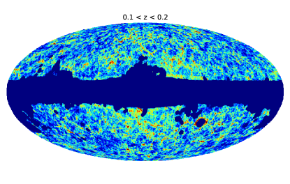
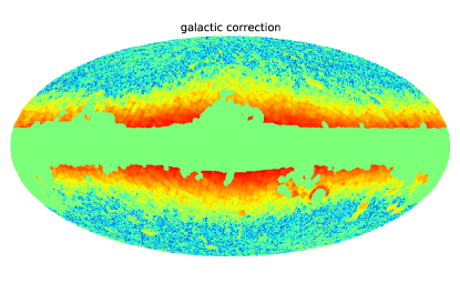
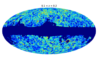
Figure 1: Illustrating the removal of residual stellar contamination from one of the WI$\times$SC tomographic slices by correlating galaxy density with total (star-dominated) WISE surface density. Only the $0.1<z<0.2$ slice is illustrated, but the same procedure was applied to all slices. The top image shows the galaxy surface density smoothed with 0.5^∘ FWHM, stretched between 0.5 and 2 times the mean density. The middle image shows the inferred stellar contamination, as described in the text, and the final image shows the corrected data.

The WISE $\times$ SuperCOSMOS photometric redshift catalogue (WI$\times$SC: Bilicki et al., 2016) is an extension beyond 2MPZ made by combining SCOS and WISE only. These two datasets provide a much deeper ($\sim 3\times$) galaxy sample than possible with 2MASS, and with over 20 times larger surface density, although its sky coverage useful for extragalactic science is smaller, about 70% of sky after applying the relevant masks (see Bilicki et al. 2016 for details of the construction of the WI$\times$SC mask). WI$\times$SC includes almost 20 million galaxies with $\langle z\rangle=0.2$ but having a broad $dN/dz$ reaching up to $z\sim 0.4$. The photo-$z$s were derived based on four bands $(B,R,W1,W2)$, again employing the ANNz package. In practice, the neural networks were trained on a complete calibration set from the equatorial fields of the Galaxy And Mass Assembly (GAMA: Liske et al., 2015) survey. As in the 2MPZ case, these photo-$z$s exhibit minimal mean bias but have larger average scatter of $\sigma_{\delta z/1+z}=0.035$, as expected due to the availability of half as many bands in WI$\times$SC as compared to 2MPZ.

One distinct issue affecting the WI$\times$SC dataset is stellar contamination. Despite masking areas of high stellar density and applying appropriate colour cuts, some stellar contamination remains at the few per cent level – a significantly larger issue than for the 2MPZ or SDSS samples. This contamination results largely from stellar blends producing spurious extended sources, and is thus concentrated towards the Galactic plane. Moreover, because of the distinct colours of such objects, the effects tend to be concentrated in particular photo-$z$ slices. We deduced a correction for this effect by plotting ‘galaxy’ surface density against the total WISE surface density (a good proxy for the stellar surface density), fitting a smooth nonlinear relation, and subtracting a version of the WISE total surface density map with the counts modified using this nonlinear relation, in order to predict the angular variation of the stellar contamination. The result of this process is shown in Fig. 1, and can be seen to yield cosmetically cleaner tomographic slices. In practice this cleaning has negligible quantitative impact on the cross-correlation analysis, since it affects only the lowest angular wavenumbers; nevertheless, this was an important check to carry out.

The DR12 photo-$z$ catalogue (Beck et al., 2016) is the most recent such dataset available from the SDSS, superseding earlier samples of that kind. Photo-$z$s and their error estimates, together with specific quality classes, were derived for about 200 million galaxies from the SDSS photometric catalogue, using the local linear regression technique based on a spectroscopic calibration set composed mostly of galaxies from the SDSS DR12 spectroscopy, plus several other surveys. The estimated precision of these photo-$z$s varies, and Beck et al. (2016) recommend filtering according to error classes and using only sources of class 1 and perhaps also $-1$, 2 and 3. After careful inspection of the catalogue, we have however decided not to follow these recommendations in order to guarantee uniform selection of the sample over the sky, and to maximise its surface density. The assignment to the particular classes is based on errors in the original SDSS photometry; hence, the variations in these classes are strongly correlated with the quality of observations, changing from pointing to pointing. Indeed, we have verified that if we followed the recommendations to preserve only those particular classes, the resulting sample would exhibit significant variations in depth and surface density following the SDSS scanning pattern. Moreover, a sample preselected according to the recommended classes would include only 55 million sources out of the 200 million available in total. We have thus decided to accept a poorer redshift quality in exchange for improved sampling uniformity and density. The only cut we apply on the parent sample (in addition to masking) is to require an estimate of the photo-$z$ to be given; this preserves over 185 million galaxies with $\langle z\rangle=0.44$ and $dN/dz$ reaching up to $z\sim 1$. In our analysis we however use only sources in the range of $0.1<z_{\mathrm{phot}}<0.6$: the more distant shells have a lower number density, making the cross-correlation results noisy, and it is harder to check the calibration of the distribution of true redshifts for photo-$z$ data in this regime (see section 2.1). The SDSS photometry in DR12 were obtained for a number of distinct sub-projects. In order to focus on a consistent extragalactic dataset, we applied a mask corresponding to the 9367 deg² of the BOSS project (Reid et al., 2016).

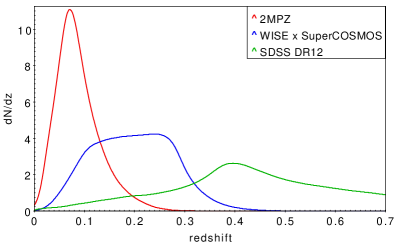
Figure 2: Normalized photometric redshift distributions of the three catalogues used in this study.

In Fig. 2 we show the photo-$z$ distributions of the three samples used in this study. Dividing this into tomographic slices is relatively arbitrary: too coarse binning limits the chance to study any evolution with redshift, but too narrow shells will lack a clear signal. In practice, we were guided by the precision of the photo-$z$s, discussed in the next section, and opted for 6 bins between $z=0.05$ and $z=0.35$ for the all-sky (2MPZ+WI$\times$SC) data, and 8 bins between $z=0.1$ and $z=0.6$ for the SDSS data. We ignore extremely local volumes where the fractional photo-$z$ errors become large. The sky distribution in these 14 tomographic slices is shown in Figs 3 & 4.

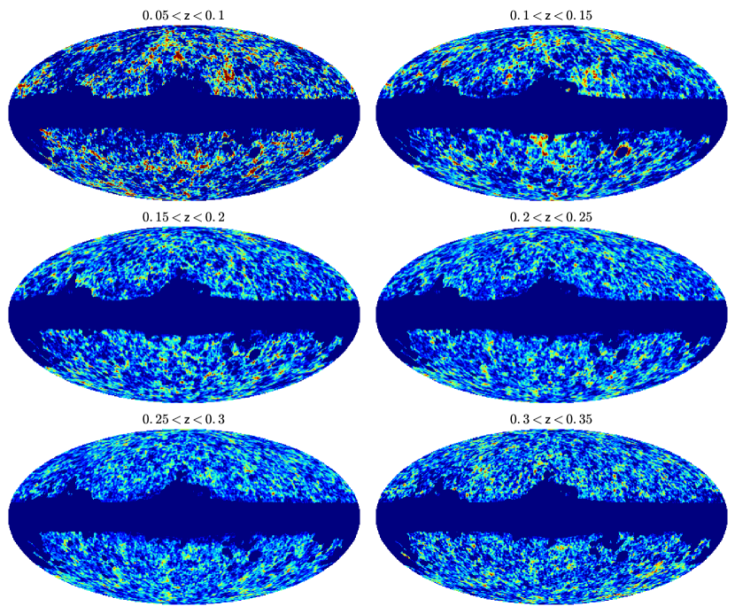
Figure 3: The galaxy surface density in various photo-$z$ slices for the 2MPZ ($0.05<z<0.1$) and WI$\times$SC (other $z$ bins), The number counts have been smoothed with a 1 degree FWHM Gaussian, and the colour scale spans 0.7 to 2 times the mean density. The WI$\times$SC slices have been corrected for residual stellar contamination as illustrated in Fig. 1.

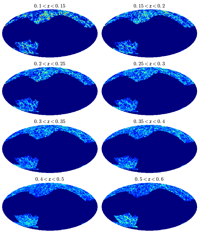
Figure 4: The equivalent of the previous figure, now using SDSS photo-$z$ data (for which no stellar correction was made). Again, the number counts have been smoothed with a 1 degree FWHM Gaussian, and the colour scale spans 0.7 to 2 times the mean density. The redshift range is larger than for WI$\times$SC, but the sky coverage is less. Although the comparison is not exact, because the SDSS photo-$z$ precision is higher, a visual inspection reveals similar LSS features in both sets of slices. This agreement is quantified in the text.

2.1 Redshift distributions

For accurate theoretical predictions, we require a good model for the probability distribution of true spectroscopic redshifts that results from a given photo-$z$ selection, $p(z)$. Photometric redshifts are generally calibrated so that the distribution of true $z$ at given $z_{\rm phot}$ is unbiased – but we still need to know the scatter in order to provide the appropriate broadening of $p(z)$.

We derive the redshift distributions of our photometric samples using overlapping spectroscopic datasets. For 2MPZ and WI$\times$SC, this is done with the same data which were employed for the photo-$z$ training. In the former catalogue this is mostly the SDSS Main Sample, while in the latter it is stage II of the Galaxy And Mass Assembly (GAMA) survey (Liske et al., 2015). For the SDSS photometric sample we also employed GAMA for photo-$z$ calibration, it is however too shallow to probe the full depth of SDSS which we use here ($z<0.6$); we thus added also information from deeper SDSS spectroscopic samples available in Data Release 13, although we note that beyond the main sample of $r<17.77$, the SDSS spectroscopic galaxies are sparsely sampled with specific colour preselections, which makes this dataset very incomplete and generally biased as a photo-$z$ calibrator.

GAMA-II covers several fields, of which three equatorial ones have a very high ($98.5\%$) spectroscopic completeness down to $r<19.8$ and include almost 200,000 galaxies at $z<0.6$ with a median $\langle z\rangle\simeq 0.2$. SDSS DR13 spectroscopic (Albareti et al., 2017) includes over 2.6 million galaxies at redshifts $z<1$, albeit not with the simple magnitude-limited selection seen in GAMA.

In order to allow for flexibility, to derive estimates of $dN/dz_{\mathrm{spec}}$ for each photo-$z$ bin we modelled the conditional distributions of the true redshift at given photometric redshift, $\delta z\equiv z_{\mathrm{spec}}-z_{\mathrm{phot}}$, as a function of redshift. Then the true redshift distributions for each bin are estimated from the photometric ones via

$$p_{s}(z_{s})=\int p_{p}(z_{p})\,p_{\delta z}(z_{s}-z_{p})\,\mathrm{d}z_{p},$$ (2)

where subscript ‘$s$’ stands for spectroscopic and ‘$p$’ for photometric. Note that this is not the same as considering the ‘photo-$z$ error distribution’, which would be the conditional distribution of photo-$z$ at given true spectroscopic redshift. This is in general biased, so that $\langle(z_{p}|z_{s})\rangle\neq z_{s}$, whereas the mean true redshift at given $z_{p}$ should be unbiased by construction. Certainly, what we require here is the conditional distribution of $z_{s}$ at given $z_{p}$: this allows us to construct the distribution of true redshifts that arises when we make a particular photometric selection.

The redshift difference distributions $p_{\delta}$ were calibrated with the aforementioned spectroscopic data, which yields an empirical error distribution based on all the objects of known redshift in any photo-$z$ bin. But to avoid binning, it is convenient to use a model for the error distribution, and we considered two options: Gaussian and modified Lorentzian. The latter takes the form

$$p_{\delta}\propto\left(1+\frac{\delta z^{2}}{2\,a\,s^{2}}\right)^{-a}\;,$$ (3)

where $a$ and $s$ are fitted parameters; such a formula represented the 2MPZ redshift residual distribution very well (see Bilicki et al. 2014). This flexible form allows us to account for both non-Gaussian wings as well as a more peaked distribution at the centre, both often being characteristics of photo-$z$ error distributions.

In the modelling we tested various levels of sophistication. As mentioned above, the photo-$z$s we use are constructed so that they are to a good approximation unbiased in the mean value of true $z$ at a given photo-$z$; thus we always assume the mean of $\delta z$ to be 0 at any redshift, and all the interest lies in the distribution of $\delta z$. The simplest yet least realistic model is to assume a Gaussian $\delta z$ with scatter evolving linearly with redshift, i.e. redshift-independent $\delta z/(1+z_{\mathrm{spec}})$. This can be then extended to a more general form of $\sigma(z)$ but still assuming a Gaussian form. A more accurate description is obtained by using the generalised Lorentzian (3), which has two free parameters controlling the scatter and the wings; here assuming linearly evolving $a(z)$ and $s(z)$ is general enough to capture the actual $\delta z$ behaviour. Finally, in the case of the SDSS photo-$z$s, Beck et al. (2016) provide estimates of rms $\delta z$ for each source, so we were able to test a model where these individual errors were used to estimate the true redshift distributions from the photometric ones. In general, this approach did not give a good agreement with the direct inference of the $\delta z$ distribution using calibrating spectroscopy; this probably reflects the fact that the SDSS error estimates are only claimed to be reliable for class 1 sources (see Beck et al. 2016 for details), whereas we make no selection on class.

For WI$\times$SC the best-fit Gaussian scatter is $\sigma(z)=0.08z+0.02$ while the Lorentzian parameters were fitted individually for each redshift bin; their redshift dependence is approximately $a(z)\simeq-4z+3$ and $s(z)\simeq 0.04z+0.02$. In the case of SDSS, calibration on SDSS spectroscopy only (dominated by LRGs) gives best-fit Gaussians with $\sigma(z)=0.02(1+z)$; more realistic modelling with GAMA (+SDSS at $z>0.4$) indicates $\sigma(z)=0.03(1+z)$; finally, if the published photo-$z$ errors from Beck et al. (2016) are used, then the overall $p_{\delta}$ can be approximated with a Gaussian of $\sigma(z)=0.05(1+z)$. Of these three models we consider the middle one to be the most realistic. For the SDSS data, we did not find that it was necessary to resort to non-Gaussian error distribution models in order to obtain a good description of the results; as might have been expected, the digital SDSS photometry is better defined and less subject to outliers than the SCOS legacy photographic measurements.

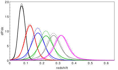
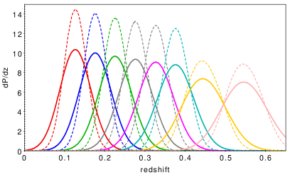
Figure 5: Calibrated redshift distributions of the 2MPZ+WI$\times$SC (upper) and SDSS DR12 catalogues (lower), derived by convolving the photo-$z$ distribution in each slice with an error distribution. In the top panel, dashed curves use a Gaussian convolving function and solid use a modified Lorentzian (adopted model). Black lines show the distributions for 2MPZ (single bin). In the lower panel, the lines are for two different Gaussians: dashed is $\sigma=0.02$ and solid is $\sigma=0.03$ (adopted model).

As far as 2MPZ is concerned, we used only one redshift bin, and we modelled its $p_{\delta}$ as either a Gaussian or a modified Lorentzian with redshift-independent parameters, in a similar way as was done for the whole 2MPZ sample in Bilicki et al. (2014). As the bin we use for 2MPZ, $0.05<z_{\mathrm{phot}}<0.1$, includes over half of all the 2MPZ galaxies and is centred almost on the median redshift of the sample, it is not surprising that the best-fit parameters of the model are here very similar to those obtained in Bilicki et al. (2014); namely, for the Gaussian $\sigma_{\delta z}=0.014$ and for the Lorentzian, $a=2.93$ and $s=0.012$. See also Balaguera-Antolínez et al. (2018) for a recent validation of 2MPZ photo-$z$ performance and of the catalogue itself.

The resulting estimates of $dN/dz_{\mathrm{spec}}$ are shown in Fig. 5. The impact of the different model choices on the lensing predictions are discussed below in section 3.2.

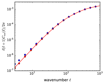
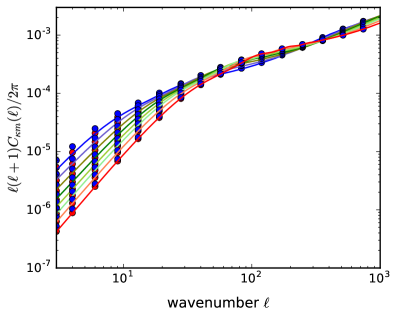
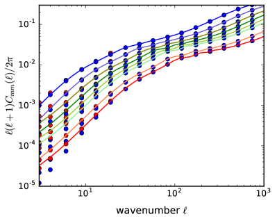
Figure 6: Theoretical predictions for the various power spectra. These plots are shown for the case of eight SDSS bins in photometric redshift, ranging between mean redshifts of 0.125 to 0.55. Red points are exact integration; blue points are the Limber–Kaiser approximation; lines show the interpolated adopted results, colour-coded from blue (lowest $z$) to red (highest $z$); the signals tend to decrease with increasing redshift. The panels show, in order: lensing auto-power; lensing-mass cross-power; mass auto-power.

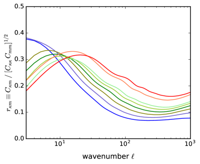
Figure 7: The harmonic-space correlation coefficient, $r_{\kappa m}$, between lensing and clustering (8), derived from the predictions of Sec. 3. This is shown for the case of the eight SDSS bins in photometric redshift, ranging between mean redshifts of 0.125 to 0.55. The lines are colour-coded from blue (lowest $z$) to red (highest $z$). Increasing redshift moves the peak to higher $\ell$ and raises the amplitude at high $\ell$.

3 Theory

The theory of CMB lensing is reviewed comprehensively by Lewis & Challinor (2006), and we summarise the key elements here. The gravitational-lens deflection is the 2D angular gradient of a potential, $\boldmath{\alpha}=\boldmath{\nabla}\psi$, where the lensing potential $\psi$ is related to the convergence, $\kappa$, via $\nabla^{2}\psi=2\kappa$ (note that Lewis & Challinor 2006 define $\psi$ with the opposite sign). Thus, in terms of angular power spectra,

$$C_{\kappa\kappa}=[\ell(\ell+1)]^{2}C_{\psi\psi}/4.$$ (4)

For a flat universe (assumed here), the CMB convergence is a projection of the fractional density fluctuation, $\delta$, with a density-dependent kernel:

$$\kappa={3H_{0}^{2}\Omega_{m}\over 2c^{2}}\int_{0}^{r_{\rm LS}}dr\;\delta(r)\;{r(r_{\rm LS}-r)\over a\,r_{\rm LS}}\equiv\int\delta(r)\;K(r)\;dr.$$ (5)

Here, $r$ is comoving distance to the element of lensing matter, and this is integrated from the origin to the last-scattering surface at $r_{\rm LS}$.

For two quantities, $a$ and $b$, obeying similar relations with kernels $K_{1}$ and $K_{2}$, the angular cross-power at multipole $\ell$ is

$$C_{ab}(\ell)=4\pi\int\Delta^{2}(k)\;d\ln k\;\int K_{1}j_{\ell}(kr)\,dr\;\int K_{2}j_{\ell}(kr)\,dr,$$ (6)

where $k$ is the comoving spatial wavenumber, $\Delta^{2}(k)$ is the dimensionless matter power spectrum, and $j_{\ell}$ is a spherical Bessel function. In the large-$\ell$ limit, the Bessel functions become sharply peaked, and we obtain a cross-power version of Kaiser’s harmonic-space version (Kaiser, 1992) of the Limber (1953) equation:

$$C_{ab}(\ell)={\pi\over\ell}\int\Delta^{2}(\ell/r)\,r\,K_{1}(r)K_{2}(r)\,dr.$$ (7)

For galaxy data, the kernel must represent the probability distribution of redshift, $p(z)$, thus $K(z)=p(z)(dr/dz)^{-1}$.

If we initially neglect galaxy bias, and assume that mass can be probed directly with the same $K(z)$ kernel, then the relevant power statistics are those relating the total CMB lensing optical depth ($\kappa$) and the projected mass ($m$) overdensity in a given photo-$z$ slice ($m$): $C_{\kappa\kappa}(\ell)$, $C_{\kappa m}(\ell)$ and $C_{mm}(\ell)$. These are illustrated in Fig. 6 for the SDSS photo-$z$ bins adopted here; the low-$z$ WI$\times$SC curves are very similar in form. These plots show that the Kaiser-Limber approximation is indistinguishable from the exact projected power of eq. (6) for $\ell\mathrel{\lower 2.58334pt\hbox{$\buildrel{\textstyle>}\over{\scriptstyle\sim}$}}20$; we therefore use this approximation at the higher multipoles where it is numerically faster and more stable than the exact expression.

It is interesting to combine these auto- and cross-power measurements into a harmonic-space correlation coefficient

$$r_{\kappa m}\equiv C_{\kappa m}\,/\,(C_{mm}C_{\kappa\kappa})^{1/2},$$ (8)

which has the interpretation that $r_{\kappa m}^{2}$ gives the fraction of the total CMB lensing variance that is contributed by the tomographic slice under consideration. This quantity is plotted in Fig. 7, where it can be seen that typical figures are 0.3 at $\ell\simeq 10$, declining to between 0.1 and 0.25 at $\ell=100$, for bins of width $\Delta z=0.05$ out to $z\sim 1$. Thus such tomographic bins can capture a significant fraction of the total lensing variance at $\ell=10$, but only a few per cent of the total variance at $\ell=100$.

3.1 Fiducial model and nonlinearities

These theoretical predictions require a choice of cosmological parameters. The best choice of these remains subject to slight debate concerning ‘tensions’ between Planck and other determinations. Our reading of the situation is that there is no conclusive evidence that any of the main determinations are in error by more than their reported statistical uncertainties. Motivated by Planck Collaboration (2016a), van Uitert et al. (2018) and DES Collaboration (2017), we adopt the following flat $\Lambda$CDM model:

$$(\Omega_{m},\Omega_{b},h,\sigma_{8},n_{s})=(0.3,0.045,0.7,0.8,0.965).$$ (9)

The remaining uncertainties in these parameters are all at the level of 2–3% (or 0.5% in $n_{s}$), which constitutes a negligible variation in the context of the current precision of the data presented here. Thus we will generally treat the $\Lambda$CDM predictions as specified perfectly by this simple fiducial model. We will then want to see how well the fiducial cross-correlation predictions agree with the measured signal. Any mismatch in amplitude can be interpreted as requiring a change in the evolving amplitude of mass fluctuation, $\sigma_{8}(z)$. A key aspect of the current analysis is that the fiducial $\sigma_{8}(z)$ is an extrapolation assuming the growth rate from standard gravity; the measured growth history inferred from the tomographic data can therefore be used to set limits on deviations from this rate. In practice, we will use the growth-index parametrisation, $f_{g}=\Omega_{m}(a)^{\gamma}$ to capture this information.

Although the lensing is weak, this does not mean that only linear scales are probed. In practice, we will work to angular multipoles of $\ell=300$, at redshifts of typically 0.2, corresponding to wavenumbers $k=0.5\,h\,{\rm Mpc}^{-1}$; nonlinear corrections are significant at these scales. We estimate these corrections using the HALOFIT code of Smith et al. (2003). More recent work has shown that the CDM simulations used to calibrate the method were systematically low in small-scale power, and revised fits were produced by Takahashi et al. (2012). A simple alternative of comparable accuracy is to correct the original predictions by the following factor, in a manner that is taken to be independent of redshift:

$$(P-P_{\rm lin})\rightarrow(P-P_{\rm lin})\times(1+2y^{2})/(1+y^{2});\quad y=k/10\,h\,{\rm Mpc}^{-1}.$$ (10)

Thus the power needs to be boosted by about a factor 2 on the very smallest scales of all; on the scales of interest here, such corrections to HALOFIT have a negligible impact.

3.2 Robustness of modelling

Beyond any uncertainties in fundamental cosmological parameters, the dominant potential source of imprecision in our lensing predictions comes from the imperfect knowledge of the true redshift distributions associated with each tomographic slice, $N(z)$. Indeed, calibration of the true redshift distribution associated with a particular photometric-redshift selection is arguably the dominant systematic in studies of weak gravitational lensing (e.g. Hildebrandt et al. 2017; Troxel et al. 2017). This is why we considered a number of different models for $dN/dz$ in Section 2.1, as shown in Fig. 5. The theoretical predictions were calculated assuming the different options from that section, asking whether the changes in the predictions were significant in the context of the statistical errors. In the interests of space we will not present multiple versions of Fig. 7. A brief summary of the findings is that the alterations in the harmonic correlation were at the few per cent level for the different models, with the exception of the simplest SDSS model based on the quoted Gaussian error from Beck et al. (2016), where the changes with respect to the direct GAMA-based calibration was at the 10% level. As will be seen below, the statistical uncertainties in the amplitude of clustering, $\sigma_{8}(z)$ are at the 5–10% level, and we are therefore confident that remaining uncertainty in photo-$z$ calibration is not important at the current level of precision.

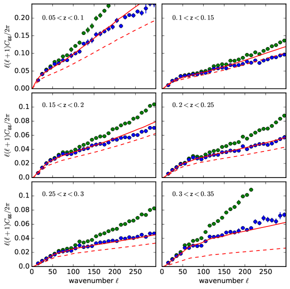
Figure 8: The angular pseudo-spectra of the various 2MPZ ($0.05<z<0.1$) and WI$\times$SC tomographic slices. The points show results without (green) and with (blue) shot-noise subtraction. The red dashed line shows the predicted angular spectrum of the nonlinear mass distribution, subject to the same $N(z)$ selection; the solid line shows the same curve linearly biased to match the data at $\ell<150$.

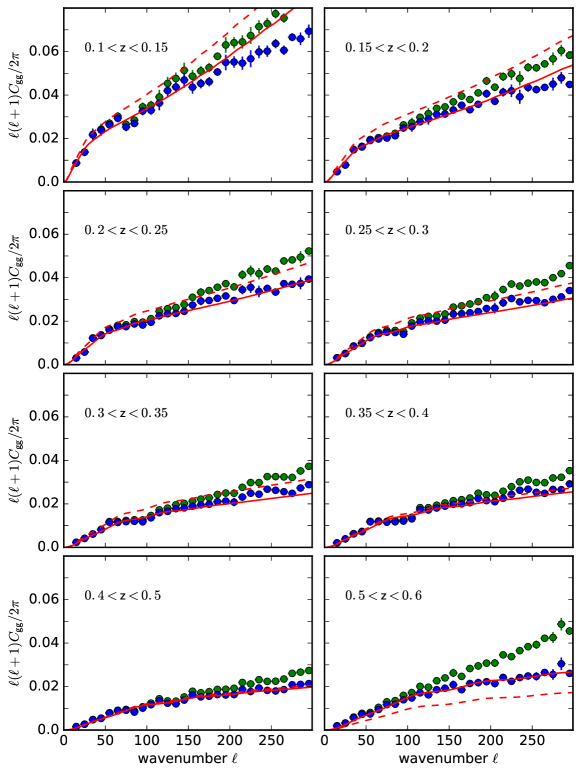
Figure 9: The angular pseudo-spectra of the various SDSS tomographic slices. The different points and lines have the same meaning as in the WI$\times$SC data of the previous figure.

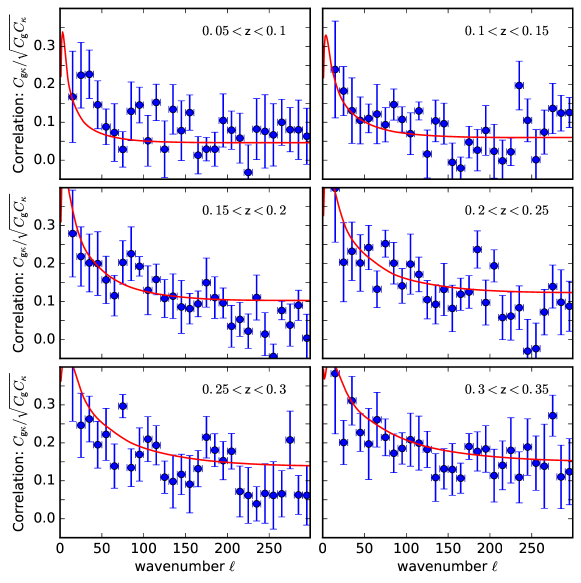
Figure 10: The harmonic-space correlation coefficient $C_{g\kappa}\,/\,(C_{gg}C_{\kappa\kappa})^{1/2}$ for the various 2MPZ+WI$\times$SC tomographic slices. $C_{g\kappa}$ and $C_{gg}$ are the direct pseudo-power estimates, and we adopt the $\Lambda$CDM theoretical prediction for $C_{\kappa\kappa}$. This statistic is independent of any degree of scale-dependent bias, $b(\ell)$, provided that it is not stochastic. A correlation is detected with high significance in all slices, for all multipoles. The lines show the theoretical prediction of our fiducial $\Lambda$CDM model, as presented in Fig. 7, taking into account the exact true redshift distributions for these slices.

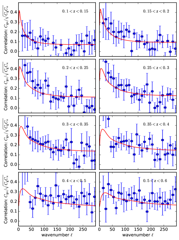
Figure 11: The harmonic-space correlation coefficient $C_{g\kappa}\,/\,(C_{gg}C_{\kappa\kappa})^{1/2}$ for the various SDSS tomographic slices. The points and lines have the same meaning as in the WI$\times$SC data of the previous figure.

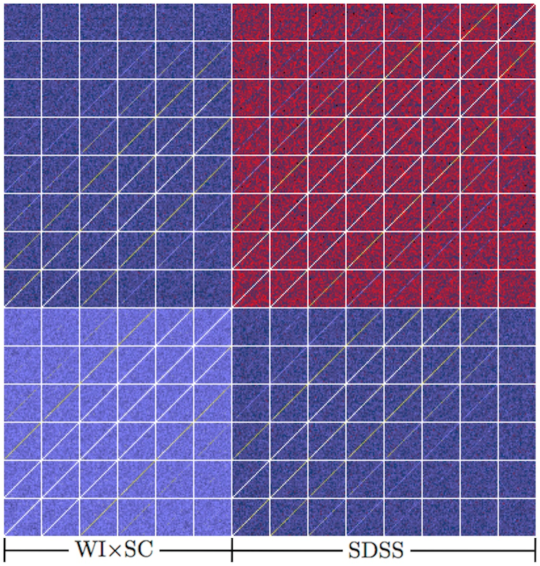
Figure 12: The correlation matrix for the CMB lensing cross-correlation measurements. Each square corresponds to a different pair of tomographic bins: the 2MPZ+WI$\times$SC bins constitute the lower left quadrant; the SDSS bins constitute the upper right. Cells increase with redshift from left to right throughout a block. The colour coding is in part to distinguish each block, rather than quantitatively encoding the correlation. As expected, we see that adjacent bins are correlated (even extending over several bin separations), and that the 2MPZ+WI$\times$SC and SDSS results are correlated where their redshift bins are at similar distances. The typical correlation coefficients are about 0.7 at one bin separation and 0.5 at two bins separation (similar in 2MPZ+WI$\times$SC and SDSS) and about 0.7 between WI$\times$SC and SDSS in the same redshift bin.

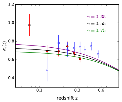
Figure 13: A plot of the fluctuation amplitude as a function of redshift, $\sigma_{8}(z)$, inferred from the amplitude of the cross-correlation results shown in Figs 10 & 11. 2MPZ and WI$\times$SC results are shown as red solid symbols; SDSS as open blue symbols. These results are derived by using the scalings from the fiducial model with assumed $\sigma_{8}=0.80$. Solid lines show expectations for different values of $gamma$ (lower $\gamma$ yields higher $\sigma_{8}(z)$).

4 Tomographic power measurements

We now need to construct auto- and cross-power estimates from our various tomographic slices to compare with the above models. This would be straightforward if we had complete sky coverage, as we would just construct the spherical-harmonic coefficients of the observable quantity under consideration, $Q$:

$$a_{\ell}^{m}=\int Q(\theta,\phi)\;Y^{*}_{\ell m}(\theta\phi)\;d\Omega,$$ (11)

where $(\theta,\phi)$ are polar angles, $Y_{\ell m}$ is a spherical harmonic, and $d\Omega$ is an element of solid angle. Here, $Q$ can be $\kappa$ or $\delta$, the surface density fluctuation in a given tomographic slice. We would then construct a direct estimator of the cross-power spectrum by averaging over $m$:

$${\hat{C}}_{\kappa\delta}=(2\ell+1)^{-1}\sum_{m=-\ell}^{m=\ell}a_{\ell}^{m}(\kappa)\,a^{*}{}_{\ell}^{m}(\delta)$$ (12)

(and similarly for the auto-power spectra). This would normally be presented as the power per $\ln\ell$:

$$\hat{\cal P}_{\kappa\delta}={\ell(\ell+1)\over 2\pi}\,{\hat{C}}_{\kappa\delta},$$ (13)

and this estimator would be suitable for direct comparison with the theory presented earlier.

The problem with this approach is that we have a mask that sets the observable to zero over some region of the sky. Thinking in Fourier language, this multiplication becomes a convolution in harmonic space, and so there is a mixing: a single $a_{\ell}^{m}$ coefficient for the direct transform of the masked data is a linear combination of the coefficients for the full sky (see section IV of Peebles 1973). But the impact of this mixing can be seen quite simply at least in the limit of modes whose effective wavelength, $2\pi/\ell$, is small compared to the scale of the mask. In equation (13), the factor $1/2\pi$ derives from the density of states – i.e. we are simply saying that the total power is the sum of the power from all the modes in a given range of $\ell$. If a fraction $f_{\rm sky}$ of the sky is masked, then the number of modes is reduced in proportion to the sky area. Hence, the power obtained from transforming the masked data is underestimated by a factor $f_{\rm sky}$. We can therefore restore the correct level of power by rescaling to obtain the pseudo-$C_{\ell}$ estimator:

$${\hat{C}}_{\kappa\delta}({\rm pseudo-}C_{\ell})={1\over f_{\rm sky}}\,{\hat{C}}_{\kappa\delta}({\rm masked})$$ (14)

(see Hivon et al. 2002). We neglect the very large-scale modes where this approximation is less accurate, $\ell<10$, which are in any case very noisy. Elsewhere, this simple approximation is adequate to much better than the precision of the measurements.

This scaling also has implications for the errors on the measurements. For Gaussian fluctuations (a reasonable approximation on most scales), the fractional power errors in each $\ell$ bin are independent and of amplitude simply $1/\sqrt{N_{\rm modes}}$, where there are $N_{\rm modes}$ modes in the bin. For masked data, these errors are therefore increased by a factor $1/\sqrt{f_{\rm sky}}$, assuming that the bin is wide in $\ell$ compared to the wavenumbers on which the transform of the mask is significant. In practice, we generate a covariance matrix so that the correlation in errors between datasets can be assessed; but for a single dataset, this mode-counting argument works very well.

Table 1: Inferred values of bias as a function of redshift in the various tomographic slices. We quote a measuring error, but it should be noted that the true error is larger, as these bias values are with respect to the fiducial model, with assumed $\sigma_{8}=0.80$.

Dataset	$\langle z\rangle$	$b(z)$
2MPZ	0.075	$1.182\pm 0.009$
WI$\times$SC	0.125	$1.086\pm 0.007$
WI$\times$SC	0.175	$1.126\pm 0.007$
WI$\times$SC	0.225	$1.144\pm 0.013$
WI$\times$SC	0.275	$1.206\pm 0.009$
WI$\times$SC	0.325	$1.548\pm 0.018$
SDSS	0.125	$0.915\pm 0.010$
SDSS	0.175	$0.894\pm 0.006$
SDSS	0.225	$0.909\pm 0.007$
SDSS	0.275	$0.902\pm 0.009$
SDSS	0.325	$0.888\pm 0.013$
SDSS	0.375	$0.966\pm 0.020$
SDSS	0.450	$0.980\pm 0.019$
SDSS	0.550	$1.245\pm 0.011$

We now present the measured pseudo-power spectra in our various tomographic slices. Figs 8 & 9 show the galaxy angular auto-power, $C_{gg}$, both the raw measurements and corrected for shot noise: $C_{\rm shot}=4\pi f_{\rm sky}/N_{g}$, where $N_{g}$ is the total number of galaxies in a given slice. These galaxy spectra are contrasted with biased non-linear mass correlations, showing that there is a weak but significant scale-dependence of bias. The degree of bias varies with redshift, tending to be anti-biased for the low-$z$ slices and moving to $b>1$ at the higher redshifts. This behaviour is reasonable: the combination of the flux limit and the redshift limits means that the more local slices must consist entirely of low luminosity galaxies, whereas the more distant slices can contain some more luminous galaxies with large bias. For completeness, we quote in Table LABEL:tab:bias the bias values inferred on the assumption of the fiducial model (fitting over $50<\ell<150$, where there is no obvious scale dependence). However, we do not use these values directly.

The existence of an a priori unknown degree of bias can be removed by constructing a harmonic-space correlation coefficient similar to (8) but using galaxy auto-power, $C_{gg}$, and galaxy-lensing cross-power, $C_{g\kappa}$, instead of mass-based statistics:

$$r_{g\kappa}=C_{g\kappa}\,/\,(C_{gg}C_{\kappa\kappa})^{1/2},$$ (15)

and we present the results in this form in Figs 10 & 11, rather than plotting the raw cross-power. Here, $C_{g\kappa}$ and $C_{gg}$ are the direct pseudo-power estimates. Although dividing by a noisy quantity is in principle undesirable, the signal-to-noise of the auto-power is very much higher than that of the cross-power, so that the auto-power measurements effectively have negligibly small random errors. The same is very much not the case for the lensing auto-power, where the cosmological signal is at best comparable to the measuring noise at $\ell\simeq 30$, and about 10 times smaller by $\ell=300$. The raw measured power spectrum of the lensing map is thus biased well above the level of the cosmological signal by the addition of the noise auto-power, and using this raw power would inevitably yield a small harmonic-space correlation – in the same way that the lensing and galaxy maps would show little correlation in configuration space, because the former is noise-dominated. We therefore choose instead to normalise our harmonic-space cross-correlation by using the $\Lambda$CDM theoretical prediction for $C_{\kappa\kappa}$. Any uncertainty in this prediction is small compared to the random errors in the cross-power, which dominate the uncertainty in the correlation measurement.

This statistic has the virtue that it is independent of any degree of scale-dependent bias, $b(\ell)$, provided that it is not stochastic. In detail, we would not expect this to be the case: on scales where nonlinearities are important, higher-order correlations affect the galaxy-galaxy and galaxy-matter correlations differently, so that we would not expect the identical $b$ to appear in $C_{g\kappa}=bC_{\kappa m}$ and $C_{gg}=b^{2}C_{mm}$. But on the scales and level of precision at which we are working, the difference is negligible (Modi et al. 2017), and so we can treat the correlation statistic $r_{g\kappa}^{2}$ as measuring empirically the fraction of the variance in $\kappa$ that is contributed by the tomographic slice being studied. Note that the immunity to scale-dependent bias is an advantage of this approach compared to a more formal method in which the data for $C_{g\kappa}$ etc. are fitted directly, with bias treated as a nuisance parameter to be marginalized over: in that case, it is necessary to assume that the bias is independent of scale (e.g. DES Collaboration 2017).

4.1 Robustness checks

4.1.1 WI$\times$SC – SDSS comparison

The WI$\times$SC data yield good detections of the galaxy-lensing cross-correlation in all tomographic bins, with a precision that is greater than the SDSS results at the same redshifts, as expected from the greater sky coverage. Given that both the legacy photographic optical data and the low-resolution WISE measurements have their issues, especially in terms of stellar contamination as discussed above, it seemed prudent to check that these measurements are free of significant systematics. We approached this by using SDSS data to create an ideal WI$\times$SC dataset within the SDSS area. Taking the known colour equations (Peacock et al., 2016), SDSS data were used to generate SuperCOSMOS $B$ and $R$ magnitudes, which were then degraded to match the measuring errors of the original photometry, as quantified by Peacock et al. (2016). This catalogue was then extinction-corrected and cut to the SuperCOSMOS limits, following which it was paired with WISE. Finally, photometric redshifts were estimated using the same ANNz code as for the real WI$\times$SC catalogue. The power spectra for this idealized catalogue were then computed and compared with the WI$\times$SC results, when restricted to the same sky coverage as SDSS. The results for the $C_{g\kappa}$ and the harmonic-space correlation were found to be in agreement to within a small fraction of the measuring error. This test is not perfect, since it is dominated by the sky region where the SuperCOSMOS data were best calibrated. The calibration was performed with DR6, but the DR12 release did not greatly extend the area of the imaging dataset (9376 deg² for the BOSS area, as opposed to 8417 deg² of legacy imaging in DR6). However, as described in Peacock et al. (2016), the calibration in the remainder of the sky was constrained primarily by optical–2MASS colours, and the reliability of this strategy could be validated using the plates with direct SDSS calibration. There should thus be no concern about the photometric calibration outside the areas with SDSS overlap. The direct WI$\times$SC–SDSS comparison is useful because it addressed the impact of other factors: poorer depth and poorer star-galaxy discrimination in the legacy photographic data. But the results of this section show that these factors do not have a significant impact on the cross-correlation statistics studied here. We therefore see no reason why the WI$\times$SC and SDSS data should not be treated as a consistent whole, with the superior depth of SDSS allowing our tomographic shells to be extended to higher redshift over a smaller area.

4.1.2 Thermal Sunyaev–Zel’dovich contamination

A distinct possible concern is that the measured tomographic cross-correlations may not reflect purely the desired cross-correlation of density and lensing convergence. This is because the CMB lensing map is constructed from non-Gaussian signatures in the temperature and polarization maps, and there are other possible non-Gaussian contributions beyond lensing. The Planck reconstruction masks out known point sources, but this process may be incomplete; in particular, there may be a contribution to the lensing reconstruction from the thermal Sunyaev–Zel’dovich (tSZ, Sunyaev & Zeldovich, 1980) signal, which will also correlate with the galaxy density. The extent of such leakage was considered by Geach & Peacock (2017), who estimated that it should bias the reconstructed $\kappa$ by only a few per cent at the location of clusters, which would be insignificant at the $S/N$ of our measurements. This effect was considered in more detail by Madhavacheril & Hill (2018), who claimed that the magnitude of the leakage increased for more massive haloes. We therefore decided to check the impact of this effect on our results empirically, as follows. We identified the 1% highest density pixels in our tomographic slices and masked them out, before repeating the cross-correlation analysis. This ‘censoring’ lowers the amplitude of galaxy clustering very substantially: a reduction in linear bias by about a factor 1.5, and a reduction in high-$\ell$ auto-power by over a factor 2. We have argued that our harmonic-space correlation measure should be independent of such scale-dependent bias effects, and indeed we found that the correlation amplitudes from this modified analysis were unchanged in amplitude to within negligible shifts of approximately 3%. This argues directly that any tSZ leakage into the lensing map at high-density regions does not cause a significant bias in our cross-correlation results.

This result can also be used to argue that other possible biases associated with nonlinear regions are negligible. The Planck lensing reconstruction works in the limit of weak deflections, and so can in principle be biased by neglected higher-order corrections. These have been estimated to alter the inferred lensing power spectrum by a few %, which would be unimportant with current data (Beck et al., 2018; Böhm et al., 2018). However, Böhm et al. (2018) also suggest that the effect of non-Gaussianity might be larger for low-$z$ cross-correlation studies, which is a possible concern. Böhm et al. (2018) leave a detailed calculation of this effect for future work, so at present we can only note that a bias associated with non-Gaussian structures would also presumably reveal itself in the most high-density regions. Thus the fact that we see no corrections when removing such regions argues that any such effect is presently unimportant. But all such biases will need to be considered more carefully with future improved lensing data.

5 Model fitting

The visual impression of Figs 10 & 11 is of good agreement between the measurements and our fiducial $\Omega_{m}=0.3$ $\Lambda$CDM model, but we now need to quantify this; thus a covariance matrix for the various measurements is required. In total there are 406 points to consider, as we have 14 tomographic bins and use 29 angular bins in each ($\Delta\ell=10$ up to a maximum $\ell=300$, but omitting the lowest bin where the pseudo-power estimate may be biased by the limited sky coverage). The most robust way to determine the covariance is by averaging over many realizations of mock data, and this is relatively easy in this case. The $S/N$ of the cross-power measurements is very much lower than the other ingredients, so we simply make Gaussian realizations of fake random lensing skies using the known total $S+N$ lensing power and correlate these with the observed galaxy data, ignoring the cosmic variance in the latter. For future work of this sort, where the lensing map is less noisy, one may want to make full realizations including properly correlated mock galaxy slices and adding their lensing signal to the CMB realizations (e.g. Xavier et al., 2016). But this level of detail would be overkill for the present application. Our simple procedure generates a covariance matrix for all the tomographic slices, shown in Fig. 12 as the correlation matrix, $C_{ij}/[C_{ii}C_{jj}]^{1/2}$. As expected from the large-area coverage, it can be seen that adjacent $\ell$ bins are uncorrelated. However, different tomographic slices are correlated via the tails of the redshift distributions.

To be used in generating a likelihood $\propto\exp(-\chi^{2}/2)$, the covariance matrix needs to be inverted. Even with a large number of data realizations, this inverse can be biased high and cause the errors on fitted parameters to be underestimated (Hartlap et al. 2007). Alternatively, one can exploit the fact that the covariance matrix is dominated by a set of diagonal lines where a given $\ell$ bin is correlated only with bins of the same $\ell$ over all the various slices. Setting the covariance to zero outside these lines gives a very well-defined inverse, and the agreement with the direct inverse is good, apart from verifying the correction in amplitude predicted by Hartlap et al. (2007). The resulting errors on the power in a given $\ell$ bin are close to the naive estimates that one would make in the absence of a covariance matrix: calculate the standard deviation in power over the modes in the bin, divide by the square root of the number of independent modes, and divide by the square root of $f_{\rm sky}$ to allow for the fact that the number of effective independent modes is reduced according to the area of sky covered.

But even though it is thus straightforward to compute the $\chi^{2}$ fit between the fiducial model and the data in a single tomographic bin, the full covariance matrix is essential in order to use all our data while allowing for the correlations induced by the overlap in redshift distributions. This overall measure of fit is completely satisfactory: $\chi^{2}=400$ for 406 degrees of freedom. We can also ask if the separate parts of the data agree with the fiducial model, computing $\chi^{2}$ for the 2MPZ+WI$\times$SC and SDSS components separately. These figures are given in Table LABEL:tab:par_fits, and are both in complete consistency with the fiducial model.

Table 2: $\chi^{2}$ values and fitted growth-rate parameters. These are derived from the cross-correlation data and models shown in Figs 10 & 11, scaling the models according to non-standard growth laws (compared to $\gamma=0.55$ and a fiducial $\Omega_{m}=0.3$), and computing $\chi^{2}$ using the covariance matrix from Fig. 12.

Dataset	$N_{\rm df}$	$\chi^{2}_{\rm min}$	parameter
2MPZ+WI$\times$SC	174	184.6	$\gamma=0.79\pm 0.19$
SDSS	232	206.5	$\gamma=0.26\pm 0.21$
All	406	400.0	$\gamma=0.77\pm 0.18$

Table 3: Inferred values of $\sigma_{8}(z)$, derived from the amplitude of the cross-correlation results shown in Figs 10 & 11. These results are derived by applying the observed ratio between our measurements and the fiducial model with assumed $\sigma_{8}=0.80$.

Dataset	$\langle z\rangle$	$\sigma_{8}(z)$
2MPZ	0.075	$0.977\pm 0.122$
WI$\times$SC	0.125	$0.691\pm 0.070$
WI$\times$SC	0.175	$0.692\pm 0.056$
WI$\times$SC	0.225	$0.745\pm 0.052$
WI$\times$SC	0.275	$0.673\pm 0.042$
WI$\times$SC	0.325	$0.608\pm 0.037$
SDSS	0.125	$0.507\pm 0.129$
SDSS	0.175	$0.809\pm 0.092$
SDSS	0.225	$0.735\pm 0.080$
SDSS	0.275	$0.752\pm 0.068$
SDSS	0.325	$0.762\pm 0.061$
SDSS	0.375	$0.728\pm 0.050$
SDSS	0.450	$0.772\pm 0.046$
SDSS	0.550	$0.682\pm 0.043$

5.1 Implications for clustering evolution

The results of the model fitting can be presented in a number of ways. The simplest is to treat each tomographic slice independently and measure the ratio between the cross-correlation signal and the fiducial prediction. Multiplying this ratio by the fiducial evolution of clustering yields an estimate of $\sigma_{8}(z)$ for that bin; these values are collected in Table LABEL:tab:sigma8 and plotted in Fig. 13. Visually, there is good overall agreement with the standard $\gamma=0.55$ model.

The detailed conditional posterior for $\gamma$ at fixed $\Omega_{m}=0.3$ is shown in Fig. 14. The overall growth index from the combined WI$\times$SC and SDSS data is slightly above the standard value: $\gamma=0.77\pm 0.18$, but a $1.2\sigma$ deviation is hardly to be regarded as surprising. This value is deduced freezing the parameters of the fiducial cosmology, as discussed earlier, although the precision on $\gamma$ is sufficiently relaxed that any uncertainty on the fiducial model is unimportant. The results for the WI$\times$SC and SDSS separately are consistent with $\gamma=0.55$ and with each other, although SDSS prefers a value below the standard one whereas the value from WI$\times$SC alone is close to the overall value. Indeed, the SDSS measurements alone are consistent with $\gamma=0$, so that a non-evolving fluctuation amplitude could not be excluded using that subset of the data. At the current level of precision, the adoption of the $\gamma$ model is thus driven as much by external theoretical considerations as by direct indications from the data. But the precision is such that the SDSS and WI$\times$SC results are not in conflict, and the overall measurements do strongly require evolution (non-zero $\gamma$). This reflects the greater WI$\times$SC sky coverage, plus the fact that the higher-$z$ SDSS data have less sensitivity to $\gamma$ (because $\Omega_{m}(z)$ approaches unity at higher $z$).

We have argued that these conclusions are not affected by the remaining uncertainties in the fiducial cosmology, but the overall theoretical framework is still critical. In particular, the $f_{g}=\Omega_{m}(z)^{\gamma}$ model implies that $\sigma_{8}(a)\propto a$ applies for $z\mathrel{\lower 2.58334pt\hbox{$\buildrel{\textstyle>}\over{\scriptstyle\sim}$}}1$, so that the expected amplitude of the cross-correlation signal near the upper limit of our data is robustly predicted from the CMB. But if we were to abandon the information in the absolute amplitude, and simply look at the relative evolution of the cross-correlation signal with redshift, then our constraints would be much less precise. This can be seen in Fig. 13, where allowing an arbitrary vertical shift in the models would clearly remove much of the sensitivity to $\gamma$.

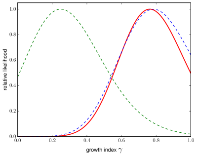
Figure 14: Conditional relative likelihoods for $\gamma$ at fixed $\Omega_{m}=0.3$. Red solid lines show the result from the total sample; dashed lines show the separate results from WI$\times$SC (blue) and SDSS (green).

6 Summary and discussion

We have presented a study of the cross-correlation between the Planck map of CMB-inferred gravitational lensing and tomographic photometric-redshift slices over $\simeq 70\%$ of the sky out to redshift $z=0.4$ derived from the 2MASS photo-$z$ data, as well as the match between WISE and the SuperCOSMOS all-sky galaxy catalogue, supplemented out to $z=0.6$ by SDSS photo-$z$ data over a smaller fraction of sky ($\simeq 25\%$). We have carried out various investigations of the robustness of these results, showing that the WI$\times$SC and SDSS datasets we use are consistent where they overlap; that the true redshift distributions in our photometric slices are known to sufficient precision; and that possible leakage of Sunyaev–Zel’dovich signal into the cross-correlation measurements is empirically negligible.

These results extend to higher redshift the similar cross-correlation study between the CMB and the local 2MASS galaxy distribution using the 2MPZ dataset (Bianchini & Reichardt 2018), and they provide coverage of a much larger area than the cross-correlation with the deeper DES data (Giannantonio et al. 2016). In fact, the ability of DES to probe to higher redshifts than the present study is of limited value. The normal assumption is that any modifications of gravity become important at low redshift (being in some way connected with the onset of cosmic acceleration), as expressed by assuming the growth-rate model $f_{g}=\Omega_{m}(z)^{\gamma}$; thus data from high redshifts, where $\Omega_{m}(z)$ is close to unity, lose all sensitivity to $\gamma$. Of course, it is still of interest to measure the high-redshift evolution, since it is always possible that we will have a major surprise and fail to validate $\delta\propto a(t)$. Nevertheless, the redshift range covered here, out to $z\simeq 0.5$, is probably the sweet spot for studies that aim to measure $\gamma$ as a proxy for testing gravity.

From this work, our overall conclusion is that we detect the contribution of low-redshift shells to the CMB lensing signal, and that the linear evolution of density over this range requires a growth index $\gamma=0.77\pm 0.18$. This measurement is consistent with the standard $\gamma=0.55$ expected in Einstein gravity, and this conclusion is in agreement with a range of other studies (e.g. Simpson et al. 2013; Mueller et al. 2018). At present, the indirect measurements of the growth rate from redshift-space distortions are more precise than the result reported here: Mueller et al. (2018) quote $\gamma=0.566\pm 0.058$. An independent cross-check is always valuable, of course, but it is interesting to ask if CMB lensing tomography could match or exceed the precision currently offered by RSD. Improvements can happen in two ways: (1) increase the volume of the tomographic shells, to suppress cosmic variance; (2) improve the $S/N$ of the lensing map, which is presently very far from being cosmic variance limited. As regards the first option, there is little that can be done at $z<0.35$, because WI$\times$SC is virtually full-sky. For the SDSS shells out to $z=0.6$, in principle the area could be expanded by a factor $\simeq 3$ (although current data from Pan-STARRS and DES would not achieve this, and further deep imaging in the far south would be needed). Even so, reducing the current errors from the SDSS slices by a factor around 1.5 would not be sufficient to pull the error on $\gamma$ below 0.1 – and as we have discussed, there is limited information to be gained on $\gamma$ by pushing to higher redshifts.

Therefore the major scope for improvement in these studies lies with the CMB. The current Planck lensing map is a tremendous achievement, but it is dominated by the effects of small-scale detector noise in the temperature and polarization maps that are used to make the reconstruction. This can be seen clearly when we compare with results from new ground-based CMB measurements. The South Pole Telescope has produced a CMB lensing reconstruction over 2500 deg² (Omori et al. 2017); as their Figure 6 shows, the SPT data alone are as accurate as Planck all-sky at $\ell=500$, so that all-sky data of SPT quality would yield an improvement in power accuracy of about a factor 4 in this regime. Next-generation experiments such as CMB S4 (Abazajian et al., 2016) will continue this trend. The improvement would be smaller at the wavenumbers of $\ell\simeq 150$, which is where the present study derives most of its signal, but we would then be able to use a wider range of wavenumbers and gain from a larger number of modes. Such a gain would come at the price of needing greater care in the treatment of nonlinearities and how these are altered by baryonic effects ($\ell=500$ corresponds to $k=1.7\,h\,{\rm Mpc}^{-1}$ at $z=0.1$). But in principle there seems no reason why CMB lensing tomography should not attain errors of a few per cent in $\gamma$. The competition from RSD will not stand still, and next-generation RSD projects such as DESI may be expected to push the errors on $\gamma$ to 1% or better (DESI Collaboration et al. 2016). But it is clear that future experiments will have ever greater concerns over systematics as their formal statistical errors shrink, and so we may expect CMB lensing tomography to play an important future role in the robust testing of Einstein gravity.

References

- Abazajian et al. (2016) Abazajian K. N., et al., 2016, preprint, (arXiv:1610.02743)
- Alam et al. (2017) Alam S., et al., 2017, MNRAS, 470, 2617
- Albareti et al. (2017) Albareti F., et al., 2017, ApJS, 233, 25
- Baker et al. (2017) Baker T., Bellini E., Ferreira P., Lagos M., Noller J., Sawicki I., 2017, Physical Review Letters, 119, 251301
- Balaguera-Antolínez et al. (2018) Balaguera-Antolínez A., Bilicki M., Branchini E., Postiglione A., 2018, MNRAS, 476, 1050
- Beck et al. (2016) Beck R., Dobos L., Budavári T., Szalay A., Csabai I., 2016, MNRAS, 460, 1371
- Beck et al. (2018) Beck D., Fabbian G., Errard J., 2018, preprint, (arXiv:1806.01216)
- Betoule et al. (2014) Betoule M., et al., 2014, A&A, 568, A22
- Bianchini & Reichardt (2018) Bianchini F., Reichardt C. L., 2018, ApJ, 862, 81
- Bianchini et al. (2016) Bianchini F., et al., 2016, ApJ, 825, 24
- Bilicki et al. (2014) Bilicki M., Jarrett T., Peacock J., Cluver M., Steward L., 2014, ApJS, 210, 9
- Bilicki et al. (2016) Bilicki M., et al., 2016, ApJS, 225, 5
- Böhm et al. (2018) Böhm V., Sherwin B. D., Liu J., Hill J. C., Schmittfull M., Namikawa T., 2018, preprint, (arXiv:1806.01157)
- Clifton et al. (2012) Clifton T., Ferreira P., Padilla A., Skordis C., 2012, Phys. Rep., 513, 1
- Collister & Lahav (2004) Collister A., Lahav O., 2004, PASP, 116, 345
- Cuoco et al. (2017) Cuoco A., Bilicki M., Xia J.-Q., Branchini E., 2017, ApJS, 232, 10
- DES Collaboration (2017) DES Collaboration 2017, preprint, (arXiv:1708.01530)
- DESI Collaboration et al. (2016) DESI Collaboration et al., 2016, preprint, (arXiv:1611.00036)
- Das et al. (2011) Das S., et al., 2011, Physical Review Letters, 107, 021301
- Doux et al. (2018) Doux C., Penna-Lima M., Vitenti S. D. P., Tréguer J., Aubourg E., Ganga K., 2018, MNRAS,
- Geach & Peacock (2017) Geach J., Peacock J., 2017, Nature Astronomy, 1, 795
- Geach et al. (2013) Geach J., et al., 2013, ApJ, 776, L41
- Giannantonio et al. (2016) Giannantonio T., et al., 2016, MNRAS, 456, 3213
- Hambly et al. (2001a) Hambly N., et al., 2001a, MNRAS, 326, 1279
- Hambly et al. (2001b) Hambly N., Irwin M., MacGillivray H., 2001b, MNRAS, 326, 1295
- Hartlap et al. (2007) Hartlap J., Simon P., Schneider P., 2007, A&A, 464, 399
- Hildebrandt et al. (2017) Hildebrandt H., et al., 2017, MNRAS, 465, 1454
- Hirata et al. (2008) Hirata C. M., Ho S., Padmanabhan N., Seljak U., Bahcall N. A., 2008, Phys. Rev. D, 78, 043520
- Hivon et al. (2002) Hivon E., Górski K., Netterfield C., Crill B., Prunet S., Hansen F., 2002, ApJ, 567, 2
- Holder et al. (2013) Holder G., et al., 2013, ApJ, 771, L16
- Jarrett et al. (2000) Jarrett T., Chester T., Cutri R., Schneider S., Skrutskie M., Huchra J., 2000, AJ, 119, 2498
- Kaiser (1992) Kaiser N., 1992, ApJ, 388, 272
- Lewis & Challinor (2006) Lewis A., Challinor A., 2006, Phys. Rep., 429, 1
- Limber (1953) Limber D., 1953, ApJ, 117, 134
- Linder (2005) Linder E., 2005, Phys. Rev. D, 72, 043529
- Linder & Cahn (2007) Linder E., Cahn R., 2007, Astroparticle Physics, 28, 481
- Liske et al. (2015) Liske J., et al., 2015, MNRAS, 452, 2087
- Madhavacheril & Hill (2018) Madhavacheril M. S., Hill J. C., 2018, preprint, (arXiv:1802.08230)
- Modi et al. (2017) Modi C., White M., Vlah Z., 2017, J. Cosmology Astropart. Phys., 8, 009
- Mueller et al. (2018) Mueller E.-M., Percival W., Linder E., Alam S., Zhao G.-B., Sánchez A., Beutler F., Brinkmann J., 2018, MNRAS, 475, 2122
- Omori et al. (2017) Omori Y., et al., 2017, ApJ, 849, 124
- Peacock et al. (2016) Peacock J., Hambly N., Bilicki M., MacGillivray H., Miller L., Read M., Tritton S., 2016, MNRAS, 462, 2085
- Peebles (1973) Peebles P., 1973, ApJ, 185, 413
- Planck Collaboration (2014) Planck Collaboration 2014, A&A, 571, A17
- Planck Collaboration (2016a) Planck Collaboration 2016a, A&A, 594, A13
- Planck Collaboration (2016b) Planck Collaboration 2016b, A&A, 594, A15
- Polarski & Gannouji (2008) Polarski D., Gannouji R., 2008, Physics Letters B, 660, 439
- Raghunathan et al. (2018) Raghunathan S., Bianchini F., Reichardt C. L., 2018, Phys. Rev. D, 98, 043506
- Reid et al. (2016) Reid B., et al., 2016, MNRAS, 455, 1553
- Sherwin et al. (2011) Sherwin B. D., et al., 2011, Physical Review Letters, 107, 021302
- Sherwin et al. (2012) Sherwin B., et al., 2012, Phys. Rev. D, 86, 083006
- Simpson et al. (2013) Simpson F., et al., 2013, MNRAS, 429, 2249
- Singh et al. (2017) Singh S., Mandelbaum R., Brownstein J., 2017, MNRAS, 464, 2120
- Skrutskie et al. (2006) Skrutskie M., et al., 2006, AJ, 131, 1163
- Smith et al. (2003) Smith R., et al., 2003, MNRAS, 341, 1311
- Smith et al. (2007) Smith K. M., Zahn O., Doré O., 2007, Phys. Rev. D, 76, 043510
- Stölzner et al. (2018) Stölzner B., Cuoco A., Lesgourgues J., Bilicki M., 2018, Phys. Rev. D, 97, 063506
- Sunyaev & Zeldovich (1980) Sunyaev R. A., Zeldovich I. B., 1980, ARA&A, 18, 537
- Takahashi et al. (2012) Takahashi R., Sato M., Nishimichi T., Taruya A., Oguri M., 2012, ApJ, 761, 152
- Troxel et al. (2017) Troxel M. A., et al., 2017, preprint, (arXiv:1708.01538)
- Wright et al. (2010) Wright E., et al., 2010, AJ, 140, 1868
- Xavier et al. (2016) Xavier H., Abdalla F., Joachimi B., 2016, MNRAS, 459, 3693
- van Engelen et al. (2012) van Engelen A., et al., 2012, ApJ, 756, 142
- van Uitert et al. (2018) van Uitert E., et al., 2018, MNRAS, 476, 4662